4.1. Creeping flow regime

The flow is set into motion when a radially injected electric current interacts with the imposed dipolar magnetic field. In the creeping flow regime ( $Q \leqslant 1$ ), the dynamics is governed by one dimensionless number, that is, the Hartmann number $Ha$ . When the Hartmann number is low, the electromagnetic interaction generates a Lorentz force, which points in the negative $\theta$ -direction and drives a rotational flow in the equatorial region between the spheres, see figure 2(a). We must note that the absolute value of the maximum velocity in the dimensionless profile is $u_{max}=0.0107$ ; for the sake of presentation, the velocity profiles of the results were renormalised with $u_{max}$ . When the Hartmann number is increased, the induced electric current also increases as established in (3.8); thus, the induced Lorentz force arises and reduces the velocity of the flow (referred to as Hartmann braking), see figure 2(b). Furthermore, we can observe that the numerical results from the full sphere code (dashed lines) agree qualitatively and quantitatively with the analytical solutions (continuous lines) for small and high $Ha$ . The latter validates the numerical code and the assumptions considered in the development of the analytical approach.

Figure 2.

Radial profiles of azimuthal velocity $u_{\theta }$ at the equatorial plane with $Q=1$ for (a) $Ha=0.1$ and (b) $Ha=60$ . Continuous lines, analytical solution (3.20); dashed lines, numerical simulations. (c) Absolute value of $u_{\theta \; max}$ as a function of the Hartmann number from the analytical solution. (d) Analytical radial profiles of the electric current densities for $Ha=60$ in dimensionless form. The dash-dotted, dashed and continuous lines denote the applied (3.7), induced (3.8) and total electric current ( $j_r = j_r^0 + j_r^i$ ), respectively.

For low-Hartmann flows (as shown in figure 2a ), such as electrolytes, the induced electric currents can be neglected. Therefore, the flow can be considered hydrodynamic even if the driving force is electromagnetic. In these conditions, the velocity profile in the core behaves as $u_{\theta } \sim r^{-3}$ , which can be derived from a balance between the diffusive and the applied Lorentz force terms. This is consistent with the analytic solution presented by Figueroa et al. (Reference Figueroa, Rojas, Rosales and Vázquez2016). In addition, two viscous layers are observed in the inner and outer spheres. However, the profile in the core is linear ( $u_{\theta } \sim r$ ) for the high Hartmann flow (figure 2b ), since now, the balance is between the diffusive and both Lorentz forces (induced and applied) terms. In this scenario, the Shercliff layers are present near the spheres because the imposed magnetic field is parallel to the walls. Considering that the thickness of the Shercliff layer scales as $Ha^{-1/2}$ (Roberts Reference Roberts1967), because the magnetic field is dipolar and varies with $r$ , the Hartmann number varies locally from $Ha=60$ close to the inner sphere to $Ha=3$ at the outer sphere; thus, the thicknesses of the boundary layer are $\delta =0.13$ and $\delta = 0.57$ at $r_i$ and $r_o$ , respectively. This is consistent with the results shown in figure 2(b). As observed in figures 2(a) and 2(b), the absolute value of the maximum azimuthal velocity $u_{\theta , \, max}$ decreases with $Ha$ due to Hartmann braking. The latter can be easily perceived in figure 2(c), where the maximum velocity is plotted as a function of the Hartmann number. Additionally, the shape of the velocity profile changes with $Ha$ , the maximum velocity location moves from the inner sphere to the outer sphere, which is not a centrifugal effect, since the magnitude of the velocity is reduced with  $Ha$ . For the low-Hartmann flow, the induced electric current is negligible and the flow is dominated by the force promoted by the applied current $j_r^0$ ; therefore, the maximum magnitude of the velocity is close to the inner sphere where the forcing is stronger, as observed by Figueroa et al. (Reference Figueroa, Rojas, Rosales and Vázquez2016) and Piedra et al. (Reference Piedra, Rojas, Rivera and Figueroa2022). In turn, for the high-Hartmann flow, the induced electric current $j_r^i$ cannot be neglected and has its maximum close to the inner sphere, see figure 2(d). Thus, the Lorentz force due to the induced electric current is stronger in this region, which promotes the maximum magnitude of the velocity shift towards the outer sphere. In figure 2(d), we can observe that the induced electric current is intense inside the Shercliff layer, reaching a maximum value, and it is weak close to the outer sphere. Furthermore, in figure 2(d), we observe that the total electric current is close to zero in the core ( $0.7 \lt r \lt 1.1$ ), which is consistent with the study reported by Stelzer et al. (Reference Stelzer, Cébron, Miralles, Vantieghem, Noir, Scarfe and Jackson2015a ).

In the creeping flow regime, the rotational flow is axisymmetric since convective effects are negligible. A more complete picture of the flow can be seen in figure 3, where a meridional map of the azimuthal velocity is displayed. For the sake of presentation, the velocity maps were renormalised with $u_{max}=0.0107$ . For the low-Hartmann flow, see figure 3(a), the velocity is intense in the equatorial zone close to the inner sphere and extends towards the polar zone. When the Hartmann number increases, as seen in figure 3(b), the overall velocity is reduced by one order of magnitude and the flow does not reach the polar zone of the inner sphere. The numerical results in figures 2 and 3 correspond to single snapshots.

Figure 3.

Contour map of azimuthal velocity $u_{\theta }$ at the meridional plane for $Q=1$ : (a) $Ha=0.1$ ; (b) $Ha=60$ . Numerical simulations.

4.2. Experimental comparison

In this subsection, we initially come up with a description of the flow under experimental conditions based on PIV observations on the free surface (the equatorial plane) and UDV measurements at different polar angles, and subsequently, the experimental data are compared with 3-D numerical simulations. As will be shown shortly, under the explored conditions, the flow dynamics is governed by two dimensionless numbers, namely the Reynolds number $Re$ and the Hartmann number $Ha$ .

Figure 4.

Velocity field at the equator: (a) $I=0.2$ A, $Re=450$ ; (b) $I=1$ A, $Re=1810$ . For the velocity scales, see figures 5(a) and 5(b). Experimental PIV observations. $Ha=240$ .

Figure 5.

(a) Azimuthal velocity profiles at the equator for different applied electrical currents. Marker lines, PIV observations; continuous lines, numerical simulations. (b) Absolute value of the maximum azimuthal velocity as a function of the applied electric current. Markers, PIV observations; continuous line, numerical simulations. (c) Radial velocity profiles at $\phi =102^{\circ }$ for different applied electric currents. Dashed lines, UDV measurements; continuous lines, numerical simulations. (d) Radial velocity profiles at different polar angles for $I=1$ A. Dashed lines, UDV measurements; continuous lines, numerical simulations.

When the mainly radial applied electric current interacts with the dipolar magnetic field, a mainly azimuthal Lorentz force is generated, which promotes an electromagnetically driven rotational flow in the gap between the spheres, as seen in figure 4. Since the experimental setting does not allow optical access to the flow, we make use of the equatorial symmetry for low current flows to fill half the spherical gap to carry out PIV observations. We must note that numerical simulations did not show differences between the flows with the sphere full $ ( 0 \leqslant \phi \leqslant \pi )$ and half-full $ ( \pi / 2 \leqslant \phi \leqslant \pi )$ , so the second option was chosen since it has the advantage of allowing PIV in the experimental observations. All PIV results presented are in the steady state. The PIV data come from time-averaged PIV fields at the equatorial plane. As the applied electric current is increased, the velocity of rotation also increases. The rotation of the fluid can be inverted by changing either the magnetic field or the injected current direction, the latter being easier. The radial profile of the azimuthal component $u_{\theta }$ is presented in figure 5(a) for different intensities of the applied electric current $I$ . Due to the no-slip condition on the spheres, we observe the maximum velocity close to the inner sphere and Shercliff layers close to the walls. For low currents, the velocity profile in the core becomes more linear as the radius $ r$ increases. This behaviour arises from the balance between the convective force and both the induced and applied Lorentz force terms, leading to $ u_{\theta } \sim r^{-5} + r$ . Additionally, the location of the maximum velocity moves closer to the outer sphere, which is consistent with figure 2(b). The maximum velocity location depends on the boundary layer width, as convective effects are larger, the maximum velocity approaches the inner sphere’s equator. For high currents, the location of the maximum velocity approaches the inner sphere equator, which agrees with figure 2(a). This can be explained if we consider that the Lorentz force is confined to the region near the inner sphere, where both the magnetic field and injected current are more intense, and decays as $r^{-5}$ (Piedra et al. Reference Piedra, Rojas, Rivera and Figueroa2022). Furthermore, the velocity profile in the core behaves as $u_{\theta } \sim r^{-2}$ , which can be inferred from a balance between the convective and the applied Lorentz force terms. This result aligns with previously reported experimental profiles (Figueroa et al. Reference Figueroa, Rojas, Rosales and Vázquez2016; Piedra et al. Reference Piedra, Rojas, Rivera and Figueroa2022; Proal et al. Reference Proal, Segura, Domínguez, Rivero and Figueroa2022). As the applied current increases, the absolute value of the maximum azimuthal velocity also increases, reaching up to $ \vert u_{\theta \; max} \vert \approx 11$ mm s $^{-1}$ for $I=1.6$ A, see figure 5(b). The Reynolds number based on the maximum velocity $Re= \vert u_{\theta \; max} \vert d / \nu$ for the applied electric currents $I=0.2$ A and $I=1.6$ A is $Re = 450$ and $Re = 2230$ , respectively. Thus, even though the flows remain in the laminar regime, in the experimental conditions, convective effects are noticeable. The interaction parameter (or Stuart number) $N = Ha^2 /Re$ , which denotes the ratio of electromagnetic to inertial forces, is $N=128$ and $N=26$ for $I=0.2$ A and $I=1.6$ A, respectively. Table 1 summarises the applied electric currents and the corresponding dimensionless numbers. Therefore, the coupling between the velocity field and the electric current is not negligible for the experimental conditions, and it reduces as the applied electric current increases. Figure 5(c) presents the experimental $u_r$ profiles for the UDV probe located at $\phi =102^{\circ }$ . As the applied electric current is increased, the amplitude of the radial velocity also increases. Note that these UDV measurements correspond to time averages of 900 s once the steady state is reached, dashed lines in the spatial-temporal UDV measurements shown in figure 6. Figure 5(d) shows the radial velocity component at different polar angles for a given applied electrical current, namely, $I=1$ A. For visualisation purposes, the dashed lines added in figures 7(a) and 7(b) denote the polar angles where UDV measurements were taken. Under the explored experimental conditions, the flow is predominantly in the azimuthal direction, as the radial motion is smaller in order of magnitude. It is worth mentioning that the maximum velocities of the $u_r$ component obtained from PIV at $\phi =90^{\circ }$ , that is, 0.1, 0.3 and 0.4 mm s $^{-1}$ for the corresponding applied currents 0.2, 0.6 and 1 A, are of the same order as the UDV measurements at $\phi =102^{\circ }$ , see figure 5(c).

The three-dimensional numerical simulations are in steady state and do not reflect the dependence on the azimuthal angle. As observed in figures 5(a)–5(d), the results from the half-sphere simulations ( $\pi / 2 \leqslant \phi \leqslant \pi$ ) agree qualitatively with the experimental observations, since velocities are of the same order as measurements, but their correspondence is not perfect. The discrepancies follow a series of unavoidable experimental errors. Concerning the PIV observations, the intrinsic error was obtained by adjusting a normal distribution to the data at the sample points; thus, the maximum error in the experimental observations was 15 $\%$ , as shown by the error bars in figure 5(a) for $I=0.2$ A. Additionally, we must note that the PIV was performed considering the motion of the bubbles at the interface between the liquid metal and the acid. For applied electric currents $I \gt 0.6$ A, the number of bubbles decreases and the PIV technique struggles to obtain smooth velocity profiles, introducing an additional error of up to 10 $\%$ , see the error bars in figure 5(a) for $I=1.4$ A. In addition, it is assumed that the bubbles adhere perfectly to the LM surface. This could not be entirely true as the LM velocity increases, since inertial effects and drag over the bubbles could increase the uncertainty, especially near the outer sphere. Finally, the optical aberration caused by the spherical geometry increases the error of the PIV observations. A simple model of this effect has been added in Appendix A. Since the optical aberration increases considerably near the outer sphere, in addition to other uncertainty sources, the PIV observations are reliable for $ r_i \leqslant r \leqslant 0.07$ m. Taking into account the latter, the line types for the profiles for $ r \gt 0.07$ m in figure 5(a) were modified (dashed). The numerical results in figure 5 were obtained from time-averaged data (100 s). Finally, it should be noted that the azimuthal velocity profiles in the symmetry plane resemble those observed in a cylindrical configuration (Stelzer et al. Reference Stelzer, Cébron, Miralles, Vantieghem, Noir, Scarfe and Jackson2015a ), with velocity magnitudes and boundary layer thicknesses of the same order of magnitude for the same Hartmann numbers.

Regarding the UDV technique, the measurements reported with the TR0405LS transducer correspond to the average velocity within an approximately cylindrical volume ${\sim} 1.7$ mm thick with a diameter of 5 mm in the outer sphere and ${\sim} 9$ mm in the inner sphere due to the divergence of the ultrasound beam. Measurements along the transducer axis are reported and are radially directed in explored configurations. Figure 6 shows the spatiotemporal distributions of the UDV measurements of the radial velocity component $u_r$ as a function of the radial coordinate $r$ at $\phi = 102^{\circ }$ for $I=0.2$ A and $I=1$ A. We can observe a transient state of approximately 320 s and 360 s for $I=0.2$ A and $I\,{=}\,1$ A, respectively, indicated by vertical dashed black lines in the plots. In the steady state, well-defined stripes are observed. The reported profiles correspond to the average value within the steady state. The error bars are considered as $\pm$ one standard deviation. The corresponding error bars were added to the UDV profiles in figures 5(c) and 5(d). We must note that error bars were added only to the profiles for the smallest and largest applied electric current as a reference. These results indicate that, in general, the numerical model can reproduce the experimental conditions explored of the EMSC flows, which remain symmetric with respect to the equatorial plane. A comparison between the experimental measurements and the analytical model is not possible, since the model is only valid for the creeping flow regime. In contrast, experimental observations confirm the existence of convective effects.

Figure 6.

Spatio-temporal distributions of $u_r$ at $\phi = 102^{\circ }$ : (a) $I=0.2$ A; (b) $I=1$ A. UDV observations. $Ha=240$ .

The general features of the flows are more clearly observed in figure 7, where the velocity maps and streamlines in the meridional plane are plotted. For low applied electric currents ( $I=0.2$ A), see figure 7(a, c, e), the flow is located mainly in the equatorial region. However, as the applied electric current increases, the magnitude of the velocity also increases and the flow extends towards the polar region because of convective effects. In general, the radial and polar velocity components are one order of magnitude smaller than the azimuthal component. The velocity map is axisymmetric and preserves symmetry with respect to the equator. However, the flow exhibits a three-dimensional structure, since radial and polar flows show regions with counter-flows. Due to the centrifugal force, a radial flow from the inner to the outer sphere is established, see figures 7(a) and 7(b). The main circular motion establishes a strong secondary flow that goes from the equator towards the poles, see the meridional streamlines in figures 7(e) and 7(f). The latter coincides with the low-conductivity study of Piedra et al. (Reference Piedra, Rojas, Rivera and Figueroa2022) and the MSC study of Figueroa et al. (Reference Figueroa, Schaeffer, Nataf and Schmitt2013). Figure 7(a)– 7(f) were obtained from from a time- (100 s) and azimuth-average.

Figure 7.

(a–d) Contour maps of the velocity components at the meridional plane. (e,f) Meridional streamlines, $U$ denotes the magnitude of the meridional velocity. First column $I=0.2$ A. Second column $I=1$ A. Dashed lines in panels (a) and (b) denote the UDV measurements shown in figures 5(c) and 5(d). Numerical simulations. $Ha=170$ .

Figure 8 shows the contour map of $j^i_{\theta }$ along with the meridional induced current lines. This figure corresponds to a time- (100 s) and azimuth-average. The azimuthal component $j^i_{\theta }$ shows a sign change according to the radial component of the velocity. As the applied electric current increases, the induced currents spread to higher latitudes; however, in the polar regions, they are close to zero. In addition, the meridional induced current lines show a quadrupolar-like distribution, that is, the current lines are perpendicular to the electrodes and tangent to the insulating regions of the inner and outer spheres. The latter quadrupolar-like distribution ensures the conservation of the charge density ( $\boldsymbol{\nabla}\boldsymbol{\cdot}\textbf {j}^{i}=0$ ). Since the induced current density vector ( $\textbf {j}^{i}$ ) is three-dimensional (see figures 9c and 9d ), the meridional current lines seem to penetrate the insulating regions of the spheres. However, in these regions, the current either bends into or out of the plane. Thus, the insulating condition ( $j_r=0$ ) is still satisfied. It is important to recall that the numerical model employs a uniform staggered mesh, which leads to a slight discrepancy between the heights of the inner and outer electrodes compared with the experimental values.

Figure 8.

Contour map of the azimuthal induced current $j^i_{\theta }$ with the meridional induced electrical current lines: (a) $I=0.2$ A; (b) $I=1$ A. Numerical simulations. $Ha=170$ .

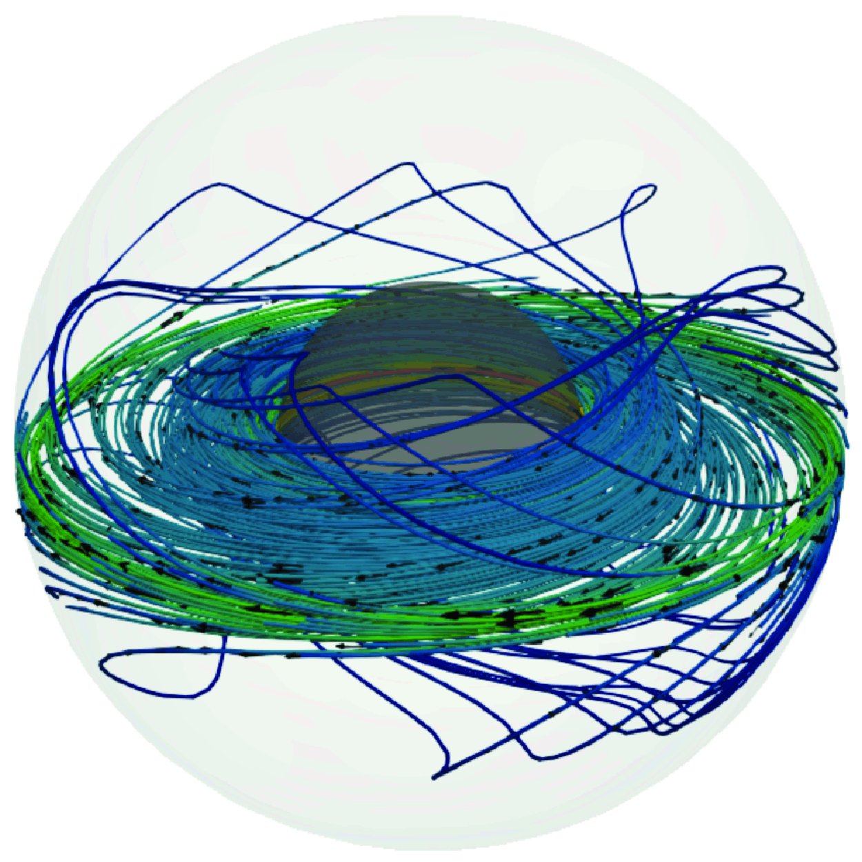
A complete picture of the flows with $I=0.2$ A and $I=1$ A can be visualised in the snapshots of numerical results shown in figure 9. For small electric currents ( $I=0.2$ A), two doughnut-shaped recirculations are observed around the equator; see figure 9(a). The flow is predominantly governed by diffusion, so the flow pattern is symmetric with respect to the equatorial plane and does not depend on the azimuthal coordinate. In the case of high electric current, see figure 9(b), convective effects dominate and the recirculation is elongated in the radial and polar directions, filling the whole gap between the spheres and displaying a full three-dimensional motion. The colour bar denotes the magnitude of the velocity $U$ in mm s $^{-1}$ for figure 9(a, b). The flow interaction with the applied magnetic field generates loops of induced electric current inside the annular gap. Figure 9(c,d) shows the paths of the induced electric current. The colour bar for figure 9(c,d) denotes the magnitude of the induced electric density current $J$ in dimensionless units. As already mentioned, the magnitude of the induced current is intense close to the inner sphere. As the applied current increases, the induced electric currents are twisted by the flow. Furthermore, the paths of the induced currents in the polar regions follow closed loops with spiral trajectories.

Figure 9.

Three-dimensional structure of the flow and the induced electrical current. (a,b) Streamlines of the velocity field for $I = 0.2$ A and $I = 1$ A. (c,d) Paths of the induced electrical current for $I = 0.2$ A and $I = 1$ A. $U$ and $J$ denote the magnitude of the velocity and the induced electrical current vectors, respectively. Numerical calculations. $Ha=170$ .

Once the numerical code was validated with both analytical and experimental results, we can explore the flow dynamics for higher applied electric currents. It is important to highlight that contrary to low-conductivity flows in concentric spheres where electromagnetically induced forces are neglected (Figueroa et al. Reference Figueroa, Rojas, Rosales and Vázquez2016; Piedra et al. Reference Piedra, Rojas, Rivera and Figueroa2022; Proal et al. Reference Proal, Segura, Domínguez, Rivero and Figueroa2022, Reference Proal, Domínguez-Lozoya, Figueroa, Rivero, Piedra and Núñez2023) and instabilities arise around $Re \approx 1500$ , here, induced effects brake the flow and instabilities are triggered at larger Reynolds numbers. It was found numerically with the full sphere code ( $0 \leqslant \phi \leqslant \pi$ ) that for a critical electric current $I \approx 9$ A ( $Re = 7880$ , $N=3.7$ ), an instability occurs and the flow becomes time dependent. Hence, the flow is no longer symmetric with respect to the equatorial plane. However, the latter is an independent study of the present work and the present study restricts the analysis of flows below this threshold.

In contrast to the mechanically forced magnetised spherical Couette flow, where the flow is induced by the drag of the rotating spheres, in this work, the flow is produced by the electromagnetic interaction of the applied electric current and the dipolar magnetic field. That is, the MSC flow is driven by a surface force, while the EMSC flow in this work is driven by a localised volumetric force that leads to different dynamics. In this context, the EMSC flow provides rich dynamics when considering other configurations. This includes factors such as the rotation of the inner and outer spheres, changing the array of the injection of the applied electric current, or even modifying both insulating or conducting boundaries.