





1. Introduction
Two-phase swirling flows are highly relevant for a number of technical applications, as they appear, for instance, in industrial cyclone separators, swirl atomisers or as a manifestation of cavitation in hydro turbines (e.g. Maly et al. Reference Maly, Cejpek, Sapik, Ondracek, Wigley and Jedelsky2021; Alligne et al. Reference Alligne, Nicolet, Tsujimoto and Avellan2014; Hreiz et al. Reference Hreiz, Gentric, Midoux, Lainé and Fünfschilling2014). In particular, the cavitating swirling flow that appears in Francis turbines under part load conditions, named the cavitating vortex rope (CVR), is a topic of important and ongoing research, both from a technical perspective, as well as in the context of modelling and stability theory. As the appearance of the CVR can tremendously impact the efficiency of Francis turbines, significant efforts have been made in order to establish a concise physical model to predict its onset and properties.
Swirling flows at high swirl are known to undergo an abrupt structural change in the flow, named vortex breakdown. It manifests in the appearance of a stagnation point along the flows’ centre line. While a number of different manifestations of vortex breakdown have been identified in the literature (see e.g. the review of Lucca-Negro & O'doherty Reference Lucca-Negro and O'doherty2001), the two most common types are the axisymmetric breakdown and the spiral breakdown that leads to the emergence of helical coherent structures in the flow. With the rise of global stability theory in the last two decades, our understanding of the dominant flow instabilities of swirling flows has substantially improved. The numerical study of laminar swirling flows, based on the Grabowski–Berger profile (Grabowski & Berger Reference Grabowski and Berger1976), conducted by Ruith et al. (Reference Ruith, Chen, Meiburg and Maxworthy2003) and the experimental study by Liang & Maxworthy (Reference Liang and Maxworthy2005) have suggested that the single and double helical structures appearing in these flows are manifestations of global modes becoming unstable through a supercritical Hopf bifurcation. This view has been confirmed by Gallaire et al. (Reference Gallaire, Ruith, Meiburg, Chomaz and Huerre2006) who performed a local stability analysis using a similar flow configuration to that of Ruith et al. (Reference Ruith, Chen, Meiburg and Maxworthy2003) and identified a single-helical unstable global mode. Considering a turbulent swirling jet with vortex breakdown, Oberleithner et al. (Reference Oberleithner, Sieber, Nayeri, Paschereit, Petz, Hege, Noack and Wygnanski2011) applied local stability analysis using the time-averaged mean flow and successfully identified a single helical global mode whose mode shape was in close correspondence to the respective experimental measurements. The destabilisation of double-helical global modes and their coexistence with single-helical modes was shown by Meliga, Gallaire & Chomaz (Reference Meliga, Gallaire and Chomaz2012), using the Grabowski–Berger profile as in Ruith et al. (Reference Ruith, Chen, Meiburg and Maxworthy2003) and Gallaire et al. (Reference Gallaire, Ruith, Meiburg, Chomaz and Huerre2006). At one combination of swirl and Reynolds number, a codimension-two point, the frequencies of these modes were approximately harmonic, thus enabling resonant behaviour. They further identified a weakly nonlinear interaction mechanism of these modes to drive the observed selection of global modes in the direct numerical simulation (DNS) study of Ruith et al. (Reference Ruith, Chen, Meiburg and Maxworthy2003). Nonlinear interaction of global modes in a Grabowski–Berger vortex has been studied by Pasche, Avellan & Gallaire (Reference Pasche, Avellan and Gallaire2018) where the appearance of a second global mode with incommensurate frequency to the primary mode led to the emergence of a quasi-periodic and chaotic dynamics. A recent study by Vanierschot et al. (Reference Vanierschot, Müller, Sieber, Percin, van Oudheusden and Oberleithner2020) found evidence on the coexistence of multiple global modes in turbulent swirling flows located in separate regions of the flow. Both modes had separate wavemakers and, despite their frequencies being harmonically related, no nonlinear interactions between them were observed.
In the context of hydro turbines, current approaches aim to describe the helical instability of the fluid flow inside the draft tube at part load conditions as a helical global mode, stemming from a linear instability mechanism. The studies of Pasche, Avellan & Gallaire (Reference Pasche, Avellan and Gallaire2017) and Müller et al. (Reference Müller, Sieber, Litvinov, Shtork, Alekseenko and Oberleithner2021) used global stability analysis around the turbulent mean flow, obtained by numerical simulation and particle image velocimetry of the flow in a model draft tube at part load, to compute linear global modes. In both works an unstable or marginally stable eigenmode was found which resembled the coherent helical structure observed in the nonlinear flow and whose frequency was in good agreement with the reference data. The successful description of the occurring helical instability through a linear instability mechanism thus gives valuable insights into its physical nature and provides an important step towards active control approaches targeting its suppression. However, the linear analyses in the referenced numerical studies are unanimously based on the assumption of a single-phase flow, thus neglecting any influence of the second fluid phase on the linear and nonlinear dynamics of the flow.
The absence of two-phase flow analyses in this matter is congruent with a general lack of global stability studies of two- and three-dimensional two-phase flows. The reasons are likely rooted in the computational costs involving such studies, as well as lacking availability of efficient linear solvers to facilitate them. Until recently, the studies of planar two-phase wake and jet flows by Tammisola et al. (Reference Tammisola, Sasaki, Lundell, Matsubara and Söderberg2011) and Tammisola, Lundell & Söderberg (Reference Tammisola, Lundell and Söderberg2012) were among the only ones that explored the global linear stability of two-phase flows. The recent article by Schmidt et al. (Reference Schmidt, Tammisola, Lesshafft and Oberleithner2021) presents, for the first time, a framework that allows for the linear global analysis of general two-phase flows by time stepping of a linearised DNS solver and is suited to explore the linear stability of two-phase swirling flows.
Given that two-phase flows potentially involve fluids of different densities or viscosities as well as an interface at which a surface tension force acts, the parameter space of any two-phase flow will be greatly increased with respect to its single-phase equivalent, thus making a general parametric analysis intractable. From this perspective, a sensible approach is to specifically investigate the influence of a single effect added to the single-phase flow. The influence of density variations in swirling flows has previously been investigated in the context of swirl combustion, where it was found that a low-density core fluid stabilises the flow (Manoharan et al. Reference Manoharan, Hansford, O'Connor and Hemchandra2015; Rukes et al. Reference Rukes, Sieber, Paschereit and Oberleithner2016). Capillary instability, driven by surface tension, is likely to have negligible influence on swirling flows under breakdown conditions as the involved time scales are much lower.
Therefore, we choose to focus on the effect of a viscosity stratification of the involved fluids as its influence on the flow dynamics is less clear. From previous studies, the potentially destabilising nature of a viscosity stratification in two-phase flows has been highlighted in the seminal work of Yih (Reference Yih1967), who found a fundamental mechanism which renders all confined interfacial shear flows with viscosity stratification linearly unstable. Similar destabilisations have been identified, among others, by Hickox (Reference Hickox1971) and Hooper & Boyd (Reference Hooper and Boyd1983). The introduction of a two-fluid flow with such stratification may therefore be expected to have considerable effects on the already complex linear and nonlinear dynamics of swirling flows.
The solver of Schmidt et al. (Reference Schmidt, Tammisola, Lesshafft and Oberleithner2021) constitutes the starting point for our analysis. We aim to shed light on the linear and nonlinear dynamics of two-phase swirling flows, particularly investigating the potentially destabilising effect of a viscosity stratification of the two immiscible phases, separated by an interface. The employed flow profile is that of the Grabowski–Berger vortex, extended to two fluid phases. We show that the introduction of a variable-viscosity flow can indeed promote destabilisation of the flow, leading to the emergence of two global modes which notably oscillate at harmonic frequencies. Subsequent bispectral analysis of the nonlinear dynamics reveals strong triadic resonance to take place in the flow at increased swirl which is rooted in the interaction of the two harmonic global modes. This leads to the emergence of multiple ultraharmonic frequencies that alter the flows periodicity. Very recently, the occurrence of synchronised oscillatory helical modes have been observed in several studies dealing with fully turbulent complex technical swirl flows in jet engine combustors and hydro turbines (Litvinov et al. Reference Litvinov, Yoon, Noren, Stöhr, Boxx and Geigle2021; Moczarski et al. Reference Moczarski, Treleaven, Oberleithner, Schmidt, Fischer and Kaiser2022). The dynamics of the investigated swirling flow may therefore be seen as a prototype for various other single or two-phase swirling flows where a similar destabilisation and interaction of multiple global modes may be observed. This is particularly relevant when developing new flow control schemes that are targeted to mitigate this dynamics.
To the best of our knowledge, the present work is the first to study the linear stability of a two-phase swirling flow. The investigated configuration focuses on the dynamics of a laminar flow and the isolated effect of a viscosity stratification. Nevertheless, we may expect its analysis to reveal important insights into the dynamics of two-phase swirling flows that translate to real-world flow scenarios that have gained attention in recent studies (Alligne et al. Reference Alligne, Nicolet, Tsujimoto and Avellan2014; Müller et al. Reference Müller, Sieber, Litvinov, Shtork, Alekseenko and Oberleithner2021).
The remainder of the paper is structured as follows: in § 2, we give a brief overview of the governing equations and numerical methodology to perform nonlinear and linear computations of immiscible two-phase flows. In § 3 we then compute nonlinear axisymmetric solutions for various flow parameters to get a general overview of how the viscosity contrast of the phases affects vortex breakdown. The axisymmetric flow states constitute the basis for the linear stability analysis which is conducted in § 4 to compute the aforementioned global modes. The linear computations are supplemented by fully three-dimensional nonlinear simulations to analyse the effect of the nonlinear triadic interaction of the unstable global modes (§ 5).
2. Numerical simulation and modal decomposition methods
2.1. Nonlinear simulation
The governing equations for an incompressible and immiscible two-phase flow are derived from their single-phase equivalents by assuming an interface of negligible thickness that separates both phases. The molecular imbalance of cohesive forces between both fluids is modelled as a surface tension force, located at the interface. The continuity and momentum equations, respectively, are given in a unified form over both fluid phases as
 \begin{gather} \partial_t \rho + \boldsymbol{u} \boldsymbol{{\cdot}}\boldsymbol{\nabla} \rho = 0, \end{gather}
 \begin{gather}\rho (\partial_t \boldsymbol{u} + \boldsymbol{u} \boldsymbol{{\cdot}}\boldsymbol{\nabla}\boldsymbol{u} ) ={-} \boldsymbol{\nabla} p + \boldsymbol{\nabla}\boldsymbol{{\cdot}} \left( 2\mu \boldsymbol{D} \right) + \sigma \kappa \boldsymbol{n} \delta(\boldsymbol{x}-\boldsymbol{x_s}) , \end{gather}
 \begin{gather}\boldsymbol{\nabla}\boldsymbol{{\cdot}} \boldsymbol{u} = 0, \end{gather}
with  $\boldsymbol {u} = (u,v,w)^{\rm T}$ the velocity vector,
 $\rho$ the density,
 $\mu$ the dynamic viscosity,
 $p$ the pressure and
 $\boldsymbol {x_s}$ being the position of the interface. The strain-rate tensor is
 $\boldsymbol {D} = (\boldsymbol {\nabla }\boldsymbol {u} + (\boldsymbol {\nabla }\boldsymbol {u})^{\rm T})/2$. Density and viscosity are represented by a Heaviside function
 $H(\boldsymbol {x}-\boldsymbol {x_s})$, that is
 $0$ in phase
 $1$ and
 $1$ in phase
 $2$ such that
 \begin{gather} \rho = \rho_{1} + H(\rho_{2} - \rho_{1}), \end{gather}
 \begin{gather}\mu = \mu_{1} + H(\mu_{2} - \mu_{1}). \end{gather}
The rightmost term in (2.1b) constitutes the surface tension where  $\sigma$ is the surface tension coefficient,
 $\kappa$ is the interface curvature,
 $\boldsymbol {n}$ is the unit normal vector of the interface and
 $\delta$ is the Dirac
 $\delta$-function that is non-zero on the interface. The surface tension is a surface force but may be converted into a volumetric force as
 \begin{equation} \sigma \kappa \boldsymbol{n} \delta(\boldsymbol{x} - \boldsymbol{x_s}) = \sigma \kappa \boldsymbol{\nabla} H(\boldsymbol{x} - \boldsymbol{x_s}). \end{equation}
From a numerical perspective, approximations of  $\delta$ and
 $H$ are given as
 $\delta _\epsilon$ and
 $H_\epsilon$, respectively, where
 $\epsilon$ is a characteristic length scale, related to the local grid size
 $\varDelta$.
Various numerical approximations for  $H_\epsilon$ may be found which are based on the continuum surface method (CSF) (Brackbill, Kothe & Zemach Reference Brackbill, Kothe and Zemach1992), where we set
 $H_\epsilon = c$ with
 $c$ being the volume fraction. This is the methodology applied in the volume-of-fluid (VOF) method (e.g. Scardovelli & Zaleski Reference Scardovelli and Zaleski1999). Similarly, for level-set (LS) methods (Sussman, Smereka & Osher Reference Sussman, Smereka and Osher1994) some smooth representation
 $H_\epsilon = f(\phi )$, based on the signed-distance function
 $\phi$ is used.
The advection of  $\rho$ in (2.1a) is equivalent to the advection of
 $c$ or
 $\phi$, respectively, and thus may be replaced by
 \begin{equation} \partial_t \psi + \boldsymbol{\nabla}\boldsymbol{{\cdot}} (\psi \boldsymbol{u})= 0 \quad \begin{cases} \psi = c & \text{if VOF}\\ \psi = \phi & \text{if LS} \end{cases}. \end{equation}
The system of (2.1) is solved with the Basilisk solver (http://basilisk.fr), using the CSF and VOF methods. We will not go into the details of computing the nonlinear surface tension term but refer to Popinet (Reference Popinet2003, Reference Popinet2009, Reference Popinet2018) where these topics are discussed extensively alongside their numerical implementations in Basilisk.
2.2. Linear stability analysis
In the context of linear stability theory, sustained coherent structures appearing in a flow may be analysed by the exponential growth of infinitesimal disturbances on a basic state flow field. To this end, the derivation of the linearised form of (2.1) follows verbatim the description in Schmidt et al. (Reference Schmidt, Tammisola, Lesshafft and Oberleithner2021). Upon non-dimensionalisation, using  $\rho _2$,
 $\mu _2$ and suitable length and velocity scales we obtain
 \begin{align} &\left[1 + H_\epsilon(\phi) \left(\frac{1}{\tilde{\rho}} -1\right)\right] (\partial_t \boldsymbol{u} + \boldsymbol{u} \boldsymbol{{\cdot}}\boldsymbol{\nabla} \boldsymbol{u} )\nonumber\\ &\quad ={-}\boldsymbol{\nabla}p + \frac{1}{Re}\boldsymbol{\nabla}\boldsymbol{{\cdot}} \left[ \left(1 + H_\epsilon(\phi) \left(\frac{1}{\tilde{\mu}} -1\right)\right) (\boldsymbol{\nabla} \boldsymbol{u} + (\boldsymbol{\nabla} \boldsymbol{u})^{\rm T}) \right] + \frac{1}{We} \kappa \boldsymbol{n} \delta_\epsilon(\phi), \end{align}
where the Reynolds number is  $Re = \rho _2 U_{{ref}} D_{{ref}} /\mu _2$, the Weber number is
 $We = \rho _2 U^2_{{ref}} D_{{ref}} /\sigma$,
 $\tilde {\rho } = \rho _1/\rho _2$ and
 $\tilde {\mu } = \mu _1/\mu _2$. Further we define the vector
 $\boldsymbol {q} = (\boldsymbol {u},p,\psi )^{\rm T}$, containing the flow variables, where
 $\psi$ may denote either
 $c$ or
 $\phi$ as required.
The quantities in (2.5) are expanded as,  $\boldsymbol {q} = \boldsymbol {Q} + \xi \boldsymbol {q'}$, where
 $\boldsymbol {Q} = (\boldsymbol {U},\varPsi )^{\rm T}$ is the basic state and
 $\boldsymbol {q}' = (\boldsymbol {u}',p',\psi ')^{\rm T}$ is a disturbance, with
 $0 < \xi \ll 1$. The disturbances are composed of normal modes
 \begin{equation} \boldsymbol{q}' (x,y,z,t) =\boldsymbol{\hat{q}}^l (x,y,z) {\rm e}^{\sigma t} + \mathrm{c.c.} \end{equation}
where  $\hat {\boldsymbol {q}}^l$ denotes the complex amplitude function and
 $\sigma$ the associated complex eigenvalue, c.c. is the complex conjugate. The growth rate and frequency of the modes are given as
 $\text {Re}(\sigma )$ and
 $\omega ^l = \mathrm {Im}(\sigma )$, respectively. For ease of reading we will denote individual normal modes by their frequency
 $\omega ^l$ and a suitable index. At leading order, the resulting linear disturbance equations in a LS formulation are then given as
 \begin{align} &\left[1 + H_\epsilon(\varPhi) \left(\frac{1}{\tilde{\rho}} -1\right)\right] (\partial_t \boldsymbol{u'} + \boldsymbol{u'} \boldsymbol{{\cdot}} \boldsymbol{\nabla} \boldsymbol{U} + \boldsymbol{U} \boldsymbol{{\cdot}} \boldsymbol{\nabla} \boldsymbol{u'} ) + 2\left[\delta_\epsilon(\varPhi)\phi'\left(\frac{1}{\tilde{\rho}} -1\right)\right](\boldsymbol{U} \boldsymbol{{\cdot}} \boldsymbol{\nabla} \boldsymbol{U})\nonumber\\ &\quad ={-}\boldsymbol{\nabla} p' + \frac{1}{Re} \boldsymbol{\nabla} \boldsymbol{{\cdot}}\left[ \left(1 + H_\epsilon(\varPhi)\left(\frac{1}{\tilde{\mu}} -1\right)\right) \left( \boldsymbol{\nabla} \boldsymbol{u'} + (\boldsymbol{\nabla} \boldsymbol{u})^{\rm T} \right) \right] \nonumber\\ &\qquad + \frac{1}{Re} \boldsymbol{\nabla}\boldsymbol{{\cdot}} \left[ \delta_\epsilon(\varPhi)\phi'\left(\frac{1}{\tilde{\mu}} -1\right) \left( \boldsymbol{\nabla} \boldsymbol{U} + (\boldsymbol{\nabla}\boldsymbol{u})^{\rm T}\right) \right] + \boldsymbol{F}_{s}(\varPhi,\phi'), \end{align}
 \begin{gather} \partial_t \phi' + \boldsymbol{\nabla}\boldsymbol{{\cdot}} (\varPhi \boldsymbol{u'}) + \boldsymbol{\nabla}\boldsymbol{{\cdot}} (\phi' \boldsymbol{U}) = 0, \end{gather}
 \begin{gather} \boldsymbol{\nabla}\boldsymbol{{\cdot}}\boldsymbol{u'} = 0. \end{gather}
The linearised momentum equation (2.7a) for interfacial two-phase flows contains several additional terms, as compared with the equation for single-phase flow which stem from the disturbances of the viscosity and density, as well as the linearised surface tension force  $\boldsymbol {F}_{s}(\varPhi,\phi ')$. These terms are described in detail in Schmidt et al. (Reference Schmidt, Tammisola, Lesshafft and Oberleithner2021). As the present study only considers a viscosity stratification, the terms involving surface tension and density perturbation are zero.
The linear system (2.7) is stated in compact form as
 \begin{equation} \frac{\partial \boldsymbol{q}'}{\partial t} = \mathcal{L}(\boldsymbol{Q})\boldsymbol{q}', \end{equation}
where  $\mathcal {L}(\boldsymbol {Q})$ is the linearised Navier–Stokes operator. Following Tuckerman & Barkley (Reference Tuckerman and Barkley2000) and Barkley, Blackburn & Sherwin (Reference Barkley, Blackburn and Sherwin2008), the system (2.8) may be reformulated as an eigenvalue problem where
 $\sigma$ and
 $\hat {\boldsymbol {q}}^l$ are the complex-valued eigenvalues and eigenmodes, respectively, and solved iteratively with an Arnoldi method.
In practice, the construction of the subspace in the Arnoldi method amounts to time stepping of the linearised equations (2.7) to obtain each Krylov vector. Following Schmidt et al. (Reference Schmidt, Tammisola, Lesshafft and Oberleithner2021), the equations (2.7) are discretised in Basilisk, similarly to the nonlinear equations. As a consequence, both the nonlinear and linear computations are facilitated using the same numerical schemes and on the same computational grid.
2.3. Flow configuration
The three-dimensional nonlinear and linear equations, (2.1) and (2.7) respectively, are solved in Cartesian coordinates on an octree-discretised grid in a cuboid domain. The total domain edge length is  $L_{tot} = 128$ and a cylindrical region with
 $0\leqslant z \leqslant Z$ and
 $0 \leqslant r \leqslant R$ is statically refined with a cell edge length of
 $\varDelta = 0.0625$ where
 $Z = 64$ and
 $R = 8$ (the convergence of the employed mesh for the linear and nonlinear analysis is demonstrated in Appendix A). The domain outside the refined cylinder is successively coarsened and indirectly acts as a sponge layer in downstream direction, by numerically diffusing vorticity and ensuring an approximately vorticity-free outflow. All length scales are non-dimensionalised with respect to the interface position at the inlet as given in (2.10). A schematic view of the domain is provided in figure 1.
Schematic view of the computational domain.

For the nonlinear flow, the parameterised Grabowski–Berger profile (Grabowski & Berger Reference Grabowski and Berger1976), with the velocity stated in cylindrical coordinates as  $\boldsymbol {u} = ( u_z, u_r, u_\theta )^{\rm T}$, is given as
 \begin{gather} u_z = \begin{cases} \alpha + (1 - \alpha)r^2(6-8r+3r^2) & \text{if}\ r \leqslant 1\\ 1 & \text{if}\ r > 1\end{cases} \end{gather}
 \begin{gather}u_\theta = \begin{cases} Sr(2-r^2) & \text{if}\ r \leqslant 1\\ S/r & \text{if}\ r > 1\end{cases} \end{gather}
 \begin{gather}u_r = 0, \end{gather}
where  $S$ is the non-dimensional swirl number which is defined as the azimuthal velocity at
 $r = 1$, relative to the axial free-stream velocity
 $S = u_\theta (r=1)/u_{z,\infty }$. The parameter
 $\alpha$ blends between jet (
 $\alpha > 1$) and wake-like (
 $\alpha < 1$) profiles of the core region
 $r \leqslant 1$ and is defined as
 $\alpha = u_z (r=0)/u_{z,\infty }$. Throughout this work, we only consider
 $\alpha = 1$, i.e. a constant axial flow profile.
The Grabowski–Berger profile was initially introduced for single-phase flow, so the extension to interfacial flow requires the definition of an interface position at the inlet  $R_{{in}}$. Derived from the parameterisation of the
 $u_z$ component, a natural choice is the radial limit of the inner core region at
 $R_{{in}} = 1$. However, different choices of
 $R_{{in}}$ will be assessed in § 3. Consequently, we define the following profiles for the volume fraction
 $c$, as well as for a LS-like passive scalar
 $\phi$, that is co-advected alongside
 $c$:
 \begin{equation} c = \begin{cases} 0 & \text{if}\ r \leqslant R_{{in}}\\ 1 & \text{if}\ r > R_{{in}}\end{cases},\quad \phi = r-R_{{in}}. \end{equation}
The profile is prescribed in Cartesian coordinates at the inlet  $\varOmega _1$, located on the left-hand side of the domain. Previous studies (e.g. Ruith et al. Reference Ruith, Chen, Meiburg and Maxworthy2003; Ruith, Chen & Meiburg Reference Ruith, Chen and Meiburg2004) have discussed the sensitivity of lateral and outflow boundary conditions on the dynamics of laminar swirling flows. Therein, convective boundary conditions are advocated to avoid reflections at the boundaries that affect the flow in the interior of the domain. However, given the grid coarsening in downstream direction for
 $z > 64$ and
 $r > 8$, in combination with a sufficiently large total domain size, we have found it sufficient to employ a standard outflow condition
 \begin{equation} \partial \boldsymbol{q}/\partial \boldsymbol{n}_\varOmega = 0, \quad p = 0, \end{equation}
imposed on the right-hand side boundary of the domain  $\varOmega _2$ where
 $\boldsymbol {n}_\varOmega$ is the unit normal vector at the domain boundary. On the lateral domain boundaries
 $\varOmega _3$ we employ symmetry conditions
 \begin{equation} \boldsymbol{u} \boldsymbol{{\cdot}} \boldsymbol{n}_\varOmega = 0, \quad \partial \psi/\partial \boldsymbol{n}_\varOmega = 0, \quad \partial (\boldsymbol{u} \boldsymbol{{\cdot}} \boldsymbol{t}_\varOmega)/\partial \boldsymbol{n}_\varOmega = 0, \end{equation}
where  $\boldsymbol {t}_\varOmega$ is the unit tangent vector.
For the linear flow, vanishing disturbances  $\hat {\boldsymbol {q}}^l = 0$ are enforced at
 $\varOmega _1$ and
 $\varOmega _2$, as well as
 $\partial \hat {\boldsymbol {p}}^l/\partial \boldsymbol {n}_\varOmega = 0$. The boundary conditions for disturbances along
 $\varOmega _3$ are similar to the nonlinear flow. Additionally, for
 $z > 64$, a damping volume force is added such that in this region the disturbances are of the form
 $\tilde {\hat {\boldsymbol {q}}}^l = \hat {\boldsymbol {q}}^l(1-\eta (z))$. The damping function is formulated as
 \begin{equation} \eta(z) = \frac{1}{2} + \frac{1}{2}\tanh{\left(\frac{z-z_0}{l}\right)}, \end{equation}
with  $z_0 = 1.25 {\cdot } 64$ and
 $l = 4$ as scaling parameters.
The basic state flow fields  $\boldsymbol {Q}$ required for the linear analysis are obtained with axisymmetric nonlinear simulations including swirl. They are performed on a two-dimensional grid in the
 $(z,r)$ plane with a symmetry condition along
 $r=0$ and by assuming zero gradients in azimuthal direction,
 ${\partial }/{\partial \theta } = 0$. The simulations are advanced towards steady state solutions until convergence with a residual
 $||\boldsymbol {u}(\hat {\boldsymbol {x}})^{n+1}-\boldsymbol {u}(\hat {\boldsymbol {x}})^{n}||_{\infty } ={O}(10^{-8})$, where
 $\hat {\boldsymbol {x}} = (0 \leqslant z \leqslant 16, 0 \leqslant r \leqslant 4)$. The axisymmetric fields are then rotated and cubically interpolated on the three-dimensional Cartesian grid, used for the linear analysis.
2.4. Modal decomposition of the nonlinear flow
2.4.1. Azimuthal Fourier decomposition
Given the rotational symmetry of the flow, the computed time-resolved fields are cubically interpolated from the computational grid in Cartesian coordinates  $(x,y,z)^{\rm T}$ onto a cylindrical grid
 $(z,r,\theta )^{\rm T}$. The interpolated fields are then decomposed into azimuthal Fourier modes
 \begin{equation} \boldsymbol{q}'(z,r,\theta,t) = \sum_{m={-}\infty}^{\infty} \boldsymbol{q}'_m(z,r,m,t) {\rm e}^{{\rm i} m \theta}, \end{equation}
with  $m$ being the azimuthal wavenumber, prior to subsequent analysis.
2.4.2. Dynamic mode decomposition
For analysis of the overall flow dynamics, the flow is decomposed into temporal modes using the dynamic mode decomposition (DMD) (Rowley et al. Reference Rowley, Mezić, Bagheri, Schlatter and Henningson2009; Schmid Reference Schmid2010). The resulting decomposition is an approximation of the Koopman operator, which is a linear infinite-dimensional operator describing a nonlinear dynamical system. Given a set of  $n$ snapshots of the flow
 $\boldsymbol {q'}^{n}$, the DMD yields a decomposition
 \begin{equation} \boldsymbol{q'}^n = \sum_{j=1}^{M-1} \lambda_j^n\hat{\boldsymbol{q}}_j + \boldsymbol{r}, \end{equation}
where  $\lambda _j^n = \exp ({{\rm i}2{\rm \pi} j/n})$ and
 $\hat {\boldsymbol {q}}_j$ are the Ritz values and vectors that approximate the Koopman modes of the dynamical system. The associated frequencies are
 $\omega = 2{\rm \pi} j/n$. The residual
 $\boldsymbol {r}$ is the result of the projection onto the subspace, spanned by
 $\boldsymbol {q'}^n$. We denote individual DMD modes by their frequency
 $\omega$ and a suitable index.
2.4.3. Sign convention for helical modes
In order to clearly categorise the spatio-temporal characteristics of the computed global modes, the sign conventions used in this work need to be clarified. The three-dimensional modes are decomposed into azimuthal wavenumbers according to (2.14) that aid in the characterisation of the structures observed in the swirling flow. Structures with  $m = 0$ are axisymmetric whereas
 $|m| > 1$ corresponds to helical structures. Helical structures, further, can be characterised by their sense of rotation and winding. The rotation refers to the temporal change of modes with respect to the base flow. This means that, for fixed
 $z$, a fluid portion on a line of constant phase circulates in time in the same direction in the
 $r\unicode{x2013}\theta$ plane as the underlying swirl if the vortex is co-rotating and in the opposite direction when the vortex is counter-rotating. The winding refers to spatial change of the modes in the
 $z$-direction. Meaning that, for fixed
 $t$ and moving in positive
 $z$, a fluid portion on a line with constant phase circulates in space in the same direction in the
 $r\unicode{x2013}\theta$ plane as the underlying swirl if the vortex is co-winding and in the opposite direction when the vortex is counter-winding.
The rotation sense from the azimuthally decomposed global modes can be inferred from the sign of the products  $\omega ^l m$. Following the sign convention in (2.6), modes with
 $\omega ^l m > 0$ are co-rotating and modes with
 $\omega ^l m < 0$ are counter-rotating. The global modes come in complex conjugate pairs. In the present flow modes with
 $\omega ^l>0$ have
 $m>0$ and modes with
 $\omega ^l<0$ have
 $m<0$. The winding sense is deduced visually from the modes and the basic flow swirl, with the result that in the present study unstable modes are co-rotating and counter-winding. Given that the modes come in complex conjugate pairs, the transformation
 $(m, \sigma ) \rightarrow (-m,-\sigma ^*)$ applies, with the asterisk denoting the complex conjugate. Thus, we can restrict ourselves to
 $m>0$ or
 $m<0$ modes without loss of generality. We choose to follow the convention used in, e.g. Oberleithner, Paschereit & Wygnanski Reference Oberleithner, Paschereit and Wygnanski2014, and only consider
 $m>0$ modes.
2.4.4. Bispectral mode decomposition
Additionally, we employ the bispectral mode decomposition (BMD) which has recently been introduced by Schmidt (Reference Schmidt2020) and is briefly summarised here, given its novelty. The BMD allows for the identification of nonlinear triadic interactions that result from a quadratic phase coupling of two frequencies. For illustration, we write (2.1) in compact form with disturbances as in (2.6)
 \begin{equation} \frac{\partial \boldsymbol{q'}}{\partial t} = \mathcal{L}(\boldsymbol{Q})\boldsymbol{q}' + \mathcal{Q}(\boldsymbol{q}',\boldsymbol{q}') +\mathcal{C}(\boldsymbol{q}',\boldsymbol{q}',\boldsymbol{q}') + S(\boldsymbol{q}'), \end{equation}
and identify four groups of terms on the right-hand side. The first term is the linear interaction between the base flow terms and a single disturbance quantity, the second term contains quadratic nonlinearities of the velocity disturbances with itself and interactions of the velocity and density or viscosity disturbances, as well as the quadratic nonlinear part of the surface tension term. The third term contains cubic interactions of the velocity and density disturbances, as well as the cubic nonlinear part of the surface tension term. The last term contains the remaining higher-order nonlinearities of the surface tension term. Consequently, triadic interactions are driven by  $\mathcal {Q}(\boldsymbol {q}',\boldsymbol {q}')$.
A triad is described by the frequency triplet  $(\omega _x,\omega _y,\omega _{x+y})$ where the frequencies
 $\omega _x$ and
 $\omega _y$ interact to form a third frequency
 $\omega _{x+y}$, obeying the condition
 $\omega _x \pm \omega _y \pm \omega _{x+y} = 0$.
The BMD constitutes an analogy to the classical bispectrum for multidimensional signals. Given a signal  $q(t)$ and the third-order moment
 $R_{qqq} = E[q(t)q(t-\tau _x)q(t-\tau _y)]$, where
 $E[{\cdot }]$ is the expectation value, the bispectrum is defined as the double Fourier transform of
 $R_{qqq}$
 \begin{align} S_{qqq}(\omega_x,\omega_y)&=\int_\infty^\infty \int_\infty^\infty R_{qqq}(\tau_x,\tau_y) \exp({-{\rm i} (\omega_x \tau_x + \omega_y \tau_y) })\,\mathrm{d}\tau_x \,\mathrm{d}\tau_y \nonumber\\ &= \lim_{T\rightarrow\infty} \frac{1}{T}E[\hat{q}(\omega_y)^*\hat{q}(\omega_x)^*\hat{q}(\omega_y+\omega_x)], \end{align}
where  $({\cdot })^*$ is the complex conjugate and
 $\hat {q}(\omega _x)$ and
 $\hat {q}(\omega _y)$ are the
 $x$th and
 $y$th frequency component of the Fourier transform of
 $\hat {q}$.
The BMD, for a multidimensional signal  $\boldsymbol {q}(\boldsymbol {x},t)$, is derived from the bispectrum as the expectation value of the spatial integral of the Fourier transforms
 $\hat {\boldsymbol {q}}_x = \hat {\boldsymbol {q}}(\boldsymbol {x},\omega _x)$,
 $\hat {\boldsymbol {q}}_y = \hat {\boldsymbol {q}}(\boldsymbol {x},\omega _y)$ and
 $\hat {\boldsymbol {q}}_{x+y} = \hat {\boldsymbol {q}}(\boldsymbol {x},\omega _{x+y})$
 \begin{equation} b(\omega_x,\omega_y) \equiv E\left[\int_\varOmega \hat{\boldsymbol{q}}_x \circ \hat{\boldsymbol{q}}_y \circ \hat{\boldsymbol{q}}_{x+y} \,\mathrm{d}\boldsymbol{x}\right], \end{equation}
where  $\circ$ denotes the element-wise product. Now, taking a number of
 $N_{blk}$ realisations of the Fourier transform
 $\hat {\boldsymbol {q}}$, the bispectral modes, representing the spatial structure of the triadic interaction, are defined as
 \begin{equation} \phi^{[i]}_{x + y} (\boldsymbol{x},\omega_{x + y}) = \sum_{j=1}^{N_{blk}} a_{ij} (\omega_{x + y})\hat{\boldsymbol{q}}^{[j]}_{x + y}. \end{equation}
The cross-frequency fields, which quantify the phase alignment of two frequencies, are given as
 \begin{equation} \phi^{[i]}_{x \circ y} (\boldsymbol{x},\omega_x,\omega_y) = \sum_{j=1}^{N_{blk}} a_{ij} (\omega_{x + y})\hat{\boldsymbol{q}}^{[j]}_{x \circ y}, \end{equation}
where  $\hat {\boldsymbol {q}}_{x \circ y} = \hat {\boldsymbol {q}}_{x} \circ \hat {\boldsymbol {q}}_{y}$. The bispectral modes are therefore linear combinations of the Fourier modes
 $\hat {\boldsymbol {q}}$ whereas the cross-frequency fields are maps of phase alignment. The mode bispectrum (2.18) is derived from the spatial integration of the element-wise product
 \begin{equation} \psi_{x,y}(\boldsymbol{x},\omega_x,\omega_y) = |\hat{\boldsymbol{q}}_{x \circ y} \circ \hat{\boldsymbol{q}}_{x + y} |, \end{equation}
which is a measure of the local bicorrelation of  $\omega _x$ and
 $\omega _y$ and hence we may call
 $\psi$ an interaction map.
The goal then is to find the coefficients  $a_{ij}$ such that the modulus of
 $b(\omega _x,\omega _y)$ in (2.18) is maximised. The result is the complex mode spectrum
 $\lambda _1(\omega _x,\omega _y)$ which quantifies the triadic interaction of the frequency triplet
 $(\omega _x,\omega _y,\omega _{x+y})$. Details on the exact algorithm may be found in Schmidt (Reference Schmidt2020).
Similar to the bispectrum of a single signal,  $S_{qqq}(\omega _x,\omega _y)$, the cross-bispectrum of up to three different signals is given as
 $S_{qrs}(\omega _x,\omega _y)$. It identifies triadic interactions acting across the involved signals. In similar fashion, the cross-BMD of three different fields
 $\boldsymbol {q},\boldsymbol {r},\boldsymbol {s}$ may be computed.
3. Steady axisymmetric breakdown states
Before we turn to the linear and nonlinear analyses of helical instability in the flow, we investigate the flows’ susceptibility to axisymmetric breakdown. As axisymmetric breakdown is often considered a prerequisite to helical destabilisation, determining the critical swirl  $S_{c}$ above which vortex breakdown occurs provides an indicator as to where helical destabilisation might occur. The governing equations for interfacial flows, as derived in § 2, lead to a notably larger parameter space as compared with a single-phase flow. While a comprehensive parameter study of interfacial swirling flows is beyond the scope of this work, it is instructive to map out some parameter combinations for axisymmetric configurations to get a clear picture when axisymmetric breakdown is promoted or inhibited.
For the rest of this work we fix  $Re = 400$, and since we are interested in the isolated effect of the viscosity variation, we assume equal densities of both phases (i.e.
 $\tilde {\rho } = 1$) and neglect the influence of surface tension (
 $We = \infty$). The remaining parameters then are
 $S$ and
 $\tilde {\mu }$.
The formation of a vortex breakdown bubble implies the development of a reverse flow region and thus can be tracked using the minimum of the axial velocity
 \begin{equation} u_{z,{min}} = \min_{t \rightarrow \infty}\{u_z|r< R,z< Z\}. \end{equation}
A stagnation point forms in the flow for  $u_{z,{min}} = 0$ and as soon as
 $u_{z,{min}}$ becomes negative, vortex breakdown occurs. In figure 2(a) the dependence of the critical swirl
 $S_{c}$ in relation to
 $\tilde {\mu }$ is plotted (blue line). The coloured area represents the breakdown regime where shades of blue indicate an inhibition of vortex breakdown and shades of red indicate a promotion of vortex breakdown with respect to the single-phase flow with
 $\tilde {\mu } = 1$. For each
 $\tilde {\mu }$, indicated by a dot in the plot, flows are computed with varying
 $S$ in increments of
 $0.01$. The plotted values of
 $S_{c}$ are the smallest ones for which a stagnation point forms in the flow which leads to vortex breakdown. It is seen that a decrease of
 $\tilde {\mu }$ from unity, i.e. an increase of the viscosity of the outer fluid, leads to a decrease of
 $S_{c}$ thus making the flow more susceptible to axisymmetric breakdown. Contrastingly, an increase of
 $\tilde {\mu }$ from unity, i.e. a decrease of the viscosity of the outer fluid, leads to an increase of
 $S_{c}$ thus making the flow less susceptible to axisymmetric breakdown. The transition from a columnar flow to vortex breakdown proceeds smoothly and without an abrupt change as can be deduced from figure 2(c) for
 $\tilde {\mu } = 0.5$.
(a) In blue: critical swirl  $S_{c}$ in relation to
 $\tilde {\mu }$ above which axisymmetric vortex breakdown (VB) is observed. Colour indicates a promotion or inhibition of vortex breakdown with respect to the single-phase flow. As black dots: configurations plotted in (c,d). (b) Influence of
 $R_{{in}}$ on the reverse flow
 $u_{z,{min}}$, for
 $(S,\tilde {\mu }) = (0.8,0.5)$. The solid and dashed black lines denote
 $u_{\theta,{in}}$ and
 $\mathrm {d} u_{\theta,{in}} / \mathrm {d}r$ respectively. (c) Minimum axial velocity
 $u_{z,{min}}$ vs
 $S$ for pre- and post-vortex breakdown states,
 $\tilde {\mu } = 0.5$. (d,e) Contour plots of
 $u_z$ of axisymmetric flows for
 $S = 0.9$ and varying
 $\tilde {\mu }$ and
 $\tilde {\mu } = 0.5$ and varying
 $S$. The interface is shown as solid white line and the
 $u_z = 0$ contour, indicating reverse flow, as dashed line. The location of the minimum of
 $u_z$ is shown as a red dot.

We now focus on configurations where the outer fluid is more viscous than the inner fluid, i.e.  $\tilde {\mu } < 1$. For further illustration of the flow at pre- and post-breakdown states, contour plots of the axial velocity field
 $u_z$ for the configurations denoted by black dots in figure 2(a) are presented in figures 2(d) and 2(e). The interface is shown as a solid white line and the
 $u_z = 0$ contour, indicating reverse flow, as a dashed line. The location of the minimum of
 $u_z$ is shown as a red dot.
Fixing the swirl at  $S = 0.9$ (thus moving horizontally along the black dots in figure 2a), the flow at
 $\tilde {\mu } = 1$ is located just inside the breakdown region. Consequently, a small region of reverse flow exists where the axial velocity becomes negative. For
 $\tilde {\mu } = 0.5, 0.1$, axisymmetric breakdown intensifies, as the bubble grows and deforms. In addition, a second recirculation area forms downstream of the first bubble. As a consequence of the bubble formations, the interface is pushed outwards in radial direction.
Now fixing  $\tilde {\mu } = 0.5$ (thus moving vertically along the black dots in figure 2a), breakdown again occurs for all presented configurations. For increased swirl, the single breakdown bubble present at
 $S = 0.8$ shows a similar behaviour as when decreasing
 $\tilde {\mu }$. It appears, however, that it converges towards a fixed size and generally remains smaller. Similarly, a second breakdown bubble forms downstream of the first one that is elongated when increasing
 $S$.
The influence of the inlet interface position  $R_{{in}}$ on the vortex breakdown formation is illustrated in figure 2(b) where the minimum axial velocity
 $u_{z,{min}}$ is plotted for
 $0.5 < R_{{in}} < 1.5$ and
 $(S,\tilde {\mu }) = (0.8,0.5)$. Values
 $u_{z,{min}} < 0$ imply a reverse flow and thus are indicative of vortex breakdown. It is seen that the radial position of the interface significantly impacts intensity of the reverse flow. For values
 $R_{{in}} > 1.2$ the influence of the second fluid phase is too weak to trigger a vortex breakdown and its effect on the flow diminishes with further increase. On the other hand, for
 $0.55 \leqslant R_{{in}} \leqslant 1.2$ the interface is sufficiently close to the vortex core to trigger a breakdown. Notably, the maximum destabilisation is not reached at the boundary of the vortex core
 $R_{{in}} = 1$ but around
 $R_{{in}} = 0.8$, which corresponds to the position of the maximum of
 $u_\theta$ at the inlet. The sharp change observed between
 $0.98 < R_{{in}} < 1.0$ can be attributed the parameterisation of the profile, as
 $\mathrm {d} u_{\theta,{in}} / \mathrm {d}r$ is not continuously differentiable
 $r = 1$. For
 $R_{{in}} < 0.55$, the interface is inside the vortex core and successively starts to weaken the formation of the breakdown bubble.
The effect of  $\tilde {\mu }$ on the formation of vortex breakdown appears somewhat counter-intuitive. As the viscosity of the core fluid, where the vortex breakdown occurs, is kept constant, a viscosity ratio
 $\tilde {\mu } < 1$ implies that the viscosity of the outer fluid is increased. Intuition would suggest that the introduction of a second phase with a larger viscosity stabilises the flow through the decrease of the local Reynolds number in the more viscous phase which is given as
 $Re_{min} = \tilde {\mu }Re$. Consequently,
 $S_{c}$ would lie somewhere between the respective values for
 $Re$ and
 $Re_{min}$ for a flow with
 $\tilde {\mu } = 1$. However, the opposite is observed, as the flow for
 $\tilde {\mu } < 1$ leads to an earlier onset of vortex breakdown.
3.1. Impact of the viscosity variation on the axisymmetric vortex breakdown
To shed light on the physical mechanism behind this destabilisation, we analyse the matching conditions of the two fluids that need to be fulfilled at the interface. These state that both the velocity and the shear stress across the interface need to be continuous. Further, the stress continuity is influenced by the viscosity. The strain-rate tensor is given as  $\boldsymbol {D} = (\boldsymbol {\nabla } \boldsymbol {u} + (\boldsymbol {\nabla } \boldsymbol {u})^{\rm T})/2$ and the deviatoric viscous stress tensor consequently is
 $\boldsymbol {T} = 2\mu \boldsymbol {D}$. In line with Qadri, Mistry & Juniper (Reference Qadri, Mistry and Juniper2013), the dominant viscous stress components in the flow are
 $r-z$ and
 $r-\theta$, corresponding to the axial and azimuthal shear. The resulting stress continuity of the considered components on both sides of the interface then is given as
 \begin{gather} \left[\!\!\left[ \frac{1}{\tilde{\mu}}\left(\frac{1}{r}\frac{\partial u_r}{\partial z} + \frac{\partial u_z}{\partial r}\right) \right]\!\!\right]_{r(c=0.5),1} = \left[\!\!\left[ \frac{1}{r}\frac{\partial u_r}{\partial z} + \frac{\partial u_z}{\partial r} \right]\!\!\right]_{r(c=0.5),2}, \end{gather}
 \begin{gather}\left[\!\!\left[ \frac{1}{\tilde{\mu}}\left(\frac{1}{r}\frac{\partial u_r}{\partial \theta} + \frac{\partial u_\theta}{\partial r} - \frac{ u_\theta}{ r} \right)\right]\!\!\right]_{r(c=0.5),1} = \left[\!\!\left[ \frac{1}{r}\frac{\partial u_r}{\partial \theta} + \frac{\partial u_\theta}{\partial r} - \frac{ u_\theta}{ r} \right]\!\!\right]_{r(c=0.5),2}, \end{gather}
where the phases are denoted by  $1$ and
 $2$ and the interface location is given by the volume fraction
 $c$ as
 $r(c=0.5)$. To illustrate the influence of the viscosity stratification on these terms, we plot their radial evolution in the far wake,
 $z = 64$, of a swirling flow with
 $S = 0.78$ which is marginally below
 $S_{c}$ for
 $\tilde {\mu } = 0.5$ and compare the profiles for
 $\tilde {\mu } = 0.5$ and
 $\tilde {\mu } = 1$. The respective plots for
 $u_z$,
 $u_\theta$,
 $\partial u_z/\partial r$ and
 $\partial u_\theta /\partial r$ are shown in figure 3. As the flow at this axial position is fully relaxed, the gradients of
 $u_r$ are negligibly small and thus ignored.
(a) Comparison of (a)  $u_z$, (b)
 $\partial u_z / \partial r$, (c)
 $u_\theta$ and (d)
 $\partial u_\theta / \partial r$ around the interface in the far wake,
 $z =64$, of pre-breakdown swirling flows with
 $S=0.78$ for
 $\tilde {\mu } = 0.5$ or
 $\tilde {\mu } = 1$ (in blue). The interface, as defined by the volume fraction
 $c$ (in black), is located in the blue area.

From (3.2) it is seen that, for a two-phase flow, the velocity gradients in the radial direction are discontinuous in order to satisfy shear stress and velocity continuity at the interface. In figure 3, this results in a slowing of  $u_z$ and
 $u_\theta$ in the less viscous core fluid. With respect to
 $u_z$, this aids the onset of vortex breakdown which requires a stagnation point in the axial velocity. Moreover, the gradient
 $\partial u_z/\partial r$ is approximately equal to the negative azimuthal vorticity
 $- \omega _\theta$. The shear stress continuity leads to a substantial increase of its magnitude which intensifies the vortex breakdown.
The effect of the interface position that was analysed in figure 2(b) is also linked to the gradient  $\partial u_z/\partial r$ and thus to
 $\omega _\theta$. For interface positions approximately between
 $R_{{in}} = 1.2$ and
 $R_{{in}} = 0.6$ its maximum increases with the radial inward movement of the interface, thus intensifying the breakdown, while for
 $R_{{in}} < 0.6$, its maximum rapidly decreases again, thus weakening the breakdown (plots not shown here). Further, for small
 $R_{{in}}$, the low vorticity of the outer fluid reaches far into the vortex core, thus hindering the formation of a breakdown bubble.
4. Linear global modes
Continuing from the analysis of the axisymmetric flow, the obtained steady breakdown states are used as a base flow to compute linear global modes of the respective flow configurations. In previous studies of single-phase swirling flows, helical destabilisation has been successfully explained through the instability of the Navier–Stokes operator, linearised around a stationary basic state (e.g. Meliga et al. Reference Meliga, Gallaire and Chomaz2012; Qadri et al. Reference Qadri, Mistry and Juniper2013). It was shown that the flow undergoes a supercritical Hopf bifurcation through the destabilisation of one or several helical global modes. In order to investigate the global linear stability of the present interfacial flow, we employ the solution procedure described in § 2.2 to compute the most unstable global modes for a selection of swirl numbers above  $S_{c} = 0.79$ with
 $\tilde {\mu } = 0.5$ (corresponding to the vertical dots in figure 2a).
The growth rates  $\mathrm {Re}(\sigma )$ and frequencies
 $\mathrm {Im}(\sigma )$ of the computed eigenvalues at each swirl number, ranging from
 $S = 0.78$ to
 $S = 1$ are shown in figure 4 where increments of
 $0.01$ are used to compute solutions between
 $0.78 \leqslant S \leqslant 0.81$. The grey shaded area marks the regime where the nonlinear flow which will be analysed in § 5, converges towards a stationary solution. Additionally, tabulated values for growth rates and frequencies of the computed eigenvalues of the linear analysis for
 $S = 0.8,0.9,1.0$ are given in table 1, as well as the frequencies of the equivalent modes from the nonlinear flow.
(a) Plot of the growth rates  $\mathrm {Re}(\sigma )$ of the unstable linear global modes
 $\omega ^l$, obtained from the linear analysis, over several
 $S$. The grey circles denote stable modes. (b) Comparison of the frequencies
 $\mathrm {Im}(\sigma )$ of the linear global modes
 $\omega ^l$ (denoted by
 $\circ$) with the limit-cycle oscillations
 $\omega$ (denoted by
 $\Diamond$) of the nonlinear flow in § 5. The dashed lines connecting the data points are printed for improved readability and should not be interpreted as a linear variation of the data.

Tabulated values of growth rates  $\mathrm {Re}(\sigma )$ and frequencies
 $\mathrm {Im}(\sigma )$ of the linear modes
 $\omega ^l$. The corresponding frequencies
 $\omega$, obtained from the nonlinear flow in § 5 are shown for comparison.

As is seen, the flow remains linearly stable to perturbations for  $S \leqslant 0.78$ but becomes unstable to two global modes,
 $\omega _1^l$ and
 $\omega _2^l$ that bifurcate simultaneously at
 $S \approx 0.79$. Their frequencies are related harmonically as
 $\omega _2^l \approx 2\omega _1^l$. For the largest investigated swirl,
 $S= 1.0$, a destabilisation of two additional modes,
 $\omega _l^l$ and
 $\omega _m^l$ is observed. Their nomenclature here is chosen in accordance with the analysis of the nonlinear flow in § 5.2 where two modes,
 $\omega _l$,
 $\omega _m$ are found that bear close resemblance to these linear modes.
The three-dimensional mode shapes of the linear modes for  $S = 0.8, 0.9, 1.0$ are plotted as velocity and LS disturbances,
 $\mathrm {Re}(\hat {u}_\theta ^l)$ and
 $\mathrm {Re}(\hat {\phi }^l)$ in figure 5. As the modes in the three-dimensional computations are not restricted to an imposed azimuthal wavenumber, they are decomposed into their azimuthal wavenumbers using the conventions described in § 2.4.1 for further clarity. In the linear framework the energy content of each mode should be exclusively associated with a single azimuthal wavenumber. The energy contained in each wavenumber is calculated via the standard
 $L_2$ norm and a pictographic bar chart is given that shows the modes’ relative energy content per azimuthal wavenumber
 $m = 0, 1, 2, 3$.
Shapes of the unstable linear global modes ( $\mathrm {Re}({\hat {u}^l}_\theta )/\max [\mathrm {Re}({\hat {u}^l}_\theta )]$ in red,
 $\mathrm {Re}(\hat {\phi }^l)/\max [\mathrm {Re}(\hat {\phi }^l)]$ in blue) at the respective swirl numbers. The pictographic bar charts show the relative contributions of the respective wavenumbers
 $m = 0,1,2,3$ (from left to right) to each mode.

The mode shapes for  $S = 0.8$ reveal that the two unstable global modes have different azimuthal wavenumbers, where
 $\omega _1^l$ has
 $m = 1$ and
 $\omega _2^l$ has
 $m = 2$. This is also seen from the single and double spiralling shape of the respective modes. Both modes are active in the wake of the breakdown bubble. For
 $S = 0.9$, the results are qualitatively similar but the modes are shifted upstream, closer to the breakdown bubble. For
 $S = 1.0$, the mode shapes of
 $\omega _1^l$ and
 $\omega _2^l$ are concentrated in the immediate vicinity of the breakdown bubble. Conversely, the newly bifurcated modes
 $\omega _l^l$ and
 $\omega _m^l$ are located in the far wake region of the flow. Both modes are double helical (
 $m = 2$). Following the sign convention for
 $m$ made in § 2.4.1, all modes shown in figure 5 are co-rotating and counter-winding with respect to the base flow swirl orientation.
To shed light on the evolution of the observed  $m=1$ and
 $m=2$ modes in the
 $(S,\tilde {\mu })$ plane, linear modes are computed for various
 $S$ below and above
 $S_c$ for
 $0.4 \leqslant \tilde {\mu } \leqslant 1$ and are displayed in figure 6(a). It is seen that the
 $m=1$ mode is the leading (first to bifurcate) mode for
 $\tilde {\mu } > 0.5$, while
 $m=2$ leads for
 $\tilde {\mu } < 0.5$. At
 $\tilde {\mu } \approx 0.5$ both modes become simultaneously unstable. The evolution of the critical curves for both modes in the plot also implies that they can be traced back to the respective modes in the single-phase flow with
 $\tilde {\mu } = 1$. Hence, we can conclude that the observed modes in the two-phase swirling flow have the same origin as the respective modes in the single-phase flow and that the underlying mechanism of destabilisation is the same.
(a) Critical curves of the observed  $m=1$ (dashed line, crosses, blueish area) and
 $m=2$ (dotted line, circles, reddish area) modes. The markers show the computed configurations from which the curves are drawn. Red markers denote stable modes while blue markers denote unstable modes. The thick black line denotes the
 $S_{c}$ curve, indicating vortex breakdown. (b) Frequency ratio of the unstable modes
 $\omega ^l_2/\omega ^l_1$ at the lowest swirl
 $S$ where both modes are linearly unstable.

The occurrence of multiple unstable modes with increasing azimuthal wavenumbers has also been observed by Meliga et al. (Reference Meliga, Gallaire and Chomaz2012) in their systematic study of single-phase swirling flows in the  $S\unicode{x2013}Re$ plane using linear and weakly nonlinear analysis to identify mechanisms of mode selection in the nonlinear flow. Starting from either an unstable
 $m = 1$ or
 $m = 2$ mode, they observe subsequent bifurcations of modes with higher wavenumbers if
 $Re$ or
 $S$ are increased. Moreover, they as well report the simultaneously bifurcation of an
 $m = 1$ and
 $m = 2$ mode at a particular
 $S{-}Re$ combination (codimension-two point) where the frequencies of both modes further show an approximate 2 : 1 resonance. A similar point is found here for
 $(S,\tilde {\mu })=(0.79,0.5)$ as can be deduced from figure 6(a), given that the critical curves of
 $m = 1$ and
 $m = 2$ cross at this configuration. The change of the leading mode from
 $m=1$ to
 $m=2$ when lowering
 $\tilde {\mu }$ is likely attributed to the deformation of the columnar and breakdown vortex states, as has also been suggested by Meliga et al. (Reference Meliga, Gallaire and Chomaz2012). It appears that the effect of lowering
 $\tilde {\mu }$ on the vortex states is similar to the effect of increasing
 $S$, namely the formation of a second vortex bubble in the wake of the primary one that then facilitates the destabilisation of an
 $m=2$ mode before the
 $m=1$ mode. At the codimension-two point the linear modes are almost exactly harmonic (
 $\omega ^l_2/\omega ^l_1 \approx 2$) as can be deduced from figure 6(b), whereas for larger and lower
 $\tilde {\mu }$ the ratio is lower.
The present linear analysis further has shown that the swirl number where both global modes bifurcate for  $\tilde {\mu } = 0.5$ coincides with the critical swirl for vortex breakdown. For larger and smaller
 $\tilde {\mu }$, the leading global mode bifurcates even slightly earlier and thus becomes unstable before vortex breakdown occurs. This is in contrast to previous studies of the single-phase Grabowski–Berger vortex at lower Reynolds numbers where usually a notable regime exists where the flow, despite axisymmetric breakdown, remains stable (e.g. Ruith et al. Reference Ruith, Chen, Meiburg and Maxworthy2003). In the present study, the Reynolds number is generally larger and therefore the azimuthal shear is sufficiently strong to overcome viscous damping and lead to a bifurcation even without the topological change from a columnar to a vortex breakdown state. A hint towards this behaviour can be deduced from figure 4(a) of Meliga et al. (Reference Meliga, Gallaire and Chomaz2012) for large Reynolds numbers.
4.1. Impact of the viscosity variation on the helical instability
Similarly to the axisymmetric flow, the critical swirl for helical destabilisation of the three-dimensional flow is reduced to  $S \approx 0.79$ for
 $\tilde {\mu } = 0.5$, in contrast to
 $S \approx 0.85$ for
 $\tilde {\mu } = 1$. Thus, it is evident that, similarly to the axisymmetric vortex breakdown, the viscosity stratification, leads to stronger destabilisation than a constant-viscosity flow at the largest local Reynolds number occurring in the two-phase flow.
The pronounced helical instability has potentially two causes: it may be purely driven by the earlier onset of vortex breakdown or additionally be promoted by a destabilisation of helical modes through the interface and viscosity stratification. Insights can be gained from the existing literature on viscosity-stratified flows. Yih (Reference Yih1967) discovered a long-wave mechanism (Yih mode or interface mode) that destabilises all confined shear flows with a viscosity stratification. Hooper & Boyd (Reference Hooper and Boyd1983), equally, found a destabilisation of short waves in viscosity-stratified open Couette flow which originates in the vicinity of the interface. Similarly, for pipe flows with concentric viscosity-stratified fluids, Hickox (Reference Hickox1971), found a destabilisation for azimuthal wavenumbers  $m = 0$ and
 $m = 1$. In all of these studies the respective flows appear stable in the absence of a viscosity stratification. A physical explanation for the phenomenon was given by Hinch (Reference Hinch1984) who argued that due to the viscosity jump, the undisturbed velocity at the disturbed interface is discontinuous. In order to satisfy shear stress continuity at the interface, a velocity disturbance is required, implying an energy transfer from the base flow to the disturbed flow. This again induces vorticity disturbances on both sides of the interface where the vorticity of the less viscous layer drives the instability. His argument given for a disturbed flow, thus, is similar to the argument given above for the steady axisymmetric vortex breakdown.
The present flow is obviously significantly more complex than the flow studied by Yih and a direct translation of the above mechanism is questionable especially in light of the fact that the observed instabilities are similar to those observed in single-phase swirling flows. Thus, the underlying destabilisation mechanism remains the same. However, it may be hypothesised that similar effects that lead to a purely viscosity-induced destabilisation, play a role in the modification of the stability properties in the present flow.
To verify this hypothesis, we again consider the shear stress continuity across the interface. The condition at the perturbed interface is equal to (3.2) with the velocities replaced by disturbance quantities. Note, that the condition in this form is strictly only valid at the perturbed interface. To obtain the full condition at the unperturbed interface, given by the base flow, a Taylor expansion has to be performed, which introduces several additional terms. A detailed derivation of this condition for the two-dimensional case is described in Tammisola et al. (Reference Tammisola, Lundell and Söderberg2012). However, to assess the hypothesis it suffices to directly compare the disturbance quantities and their gradients on both sides of the unperturbed interface. The exact condition is not needed. To evaluate whether the viscosity stratification impacts the helical instability, we consider the leading unstable mode of a flow with  $(S,\tilde {\mu }) = (0.73, 0.1)$ where a pronounced influence of the stratification should be visible if it exists. We focus on the azimuthal shear
 $r-\theta$, plot
 $u'_\theta$ and
 $\partial u'_\theta /\partial r$ across the interface in figure 7 and see that
 $\partial u'_\theta /\partial r$ indeed is discontinuous across the interface. This shows that the viscosity stratification modifies the stability of the helical mode. Hence, we conclude that the helical destabilisation of the flows investigated in this study is driven by both, the structural change of the base flow through axisymmetric breakdown, promoted by the viscosity stratification, as well as a promotion of helical instability itself by viscosity stratification.
(a) Evolution of (a)  $u'_\theta$ and (b)
 $\partial u'_\theta / \partial r$ around the interface at
 $z = 32$ of the leading mode of an unstable swirling flow with
 $(S,\tilde {\mu }) = (0.73, 0.1)$ (in blue). The disturbance amplitude is scaled arbitrarily. The interface, as defined by the volume fraction
 $c$ (in black), is located in the blue area.

5. Analysis of helical instability in the nonlinear flow
The analysis of the axisymmetric breakdown in § 3 and the linear stability analysis conducted in § 4 have shown that the introduction of a second, more viscous outer fluid has a destabilising effect on the flow, resulting in vortex breakdown at lower swirl and also in an earlier destabilisation of helical global modes on the breakdown state. Further, the linear stability analysis for  $\tilde {\mu } = 0.5$ has revealed the simultaneous destabilisation of two unstable global modes in the flow that have harmonic frequencies. It is thus to be expected that a strong synchronisation and resonance of these modes can be observed in the nonlinear flow. This is investigated in the following by performing nonlinear simulations of the flow and subsequent analysis of its dynamics.
5.1. Vortex dynamics
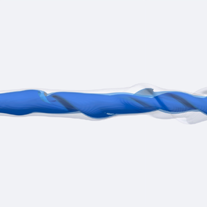
For the nonlinear simulations, we restrict the analysis to  $S>0.79$ which is beyond the bifurcation point of the two identified helical global modes (refer to figure 4). The three-dimensional simulations are initialised from the axisymmetric basic states, analysed in § 3. After initialisation, disturbances develop in the flow and lead to a loss of axisymmetry. Consequently, a spiralling motion forms in the wake of the breakdown bubble, that deforms the interface.
For a phenomenological characterisation of the flow, the vortex dynamics of the three configurations  $S = 0.8, 0.9, 1.0$ is visualised via isosurfaces of the
 $\lambda _2$-criterion (Jeong & Hussain Reference Jeong and Hussain1995) together with the fluid interface in figure 8. For each configuration the initial unstable base flow is shown as well as a snapshot of the fully developed flow. At
 $S = 0.8$, the
 $\lambda _2$ isosurfaces suggest the presence of a predominantly single-helical vortex in the low-viscosity core of the flow. In contrast, the illustration of the interface clearly shows a double-helical structure. Both spirals are synchronised in space. It therefore appears that there are two different structures, one single helical and one double helical, present in the flow which exist at harmonic frequencies as is predicted by the linear analysis. For
 $S = 0.9$, the appearance of the flow changes. The core region now leans towards a double helix whereas the overall interface deformation is single helical. The illustration of the flow at
 $S = 1.0$ shows an overall similar appearance to that of
 $S =0.9$ but reveals a more complex dynamics with several new structures appearing and disappearing in downstream development of the flow which is in line with the bifurcation of the two additional unstable linear modes at this swirl number.
Visualisation of the instantaneous flow. The upper image shows the unstable axisymmetric basic state and the lower image the fully developed flow. Isosurfaces: interface ( $c = 0.5$, in translucent grey) and vortical structures (
 $\lambda _2 = -0.5$, in dark blue;
 $\lambda _2 = -0.25$, in light translucent blue).

5.2. Modal analysis
5.2.1. Mode spectra
To gain more detailed insights on the nonlinear dynamics of the flow, a spectral analysis of the configurations  $S = 0.8, 0.9, 1.0$ with
 $\tilde {\mu } = 0.5$ using a DMD is performed. A sequence composed of
 $n=1024$ consecutive snapshots of
 $\boldsymbol {q}'$ every
 $\Delta t = 0.5$ is used for computation of the Ritz values
 $\lambda _j^n$ once the flow has reached a stable limit cycle. The resulting amplitude spectra are presented in figure 9(a). Further, a comparison of the frequencies of the linear modes
 $\omega ^l$ and the corresponding nonlinear modes
 $\omega$ is given in table 1 and figure 4(b).
(a) Magnitude of the DMD modes per frequency, extracted from the nonlinear simulation. (b) Magnitude of the DMD modes per frequency and streamwise stations every  $\Delta z = 10$. The colours denote the different wavenumbers. The peaks of the annotated modes are marked by
 ${\circ }$ (red). (c) The spatial mode shapes (
 $\mathrm {Re}(\hat {u}_\theta$) in red,
 $\mathrm {Re}(\hat {\phi })$ in blue) corresponding to the annotated modes in (a). The pictographic bar charts show the relative contributions of the respective wavenumbers
 $m = 0,1,2,3$ (from left to right) to each mode.

The spectrum obtained for  $S = 0.8$ shows two dominant frequency peaks,
 $\omega _1$ and
 $\omega _2$ which are in close agreement with the global modes
 $\omega _1^l$ and
 $\omega _2^l$ found in the linear analysis. Both modes have similar amplitudes. For convenience, we denote this set of frequencies as
 $\omega _\iota$ with
 $\iota = 1,2,3,\dots$
Increasing the swirl number to  $S = 0.9$, results in an overall similar spectrum where now, however,
 $\omega _1$ is clearly the most energetic frequency. The analysis at
 $S = 1.0$ reveals a significantly richer set of frequencies appearing in the spectrum. Apart from the frequencies contained in
 $\omega _\iota$ multiple new peaks appear which are ultraharmonic frequencies with respect to
 $\omega _\iota$ (their frequency ratios with respect to
 $\omega _1$ may be found in Appendix B). These are created through nonlinear interactions in the flow. We denote the resulting set as
 $\omega _\kappa$ where
 $\kappa =a,b,c,\ldots, n$. The mode
 $\omega _1$ is again the most energetic mode.
5.2.2. Streamwise mode spectra and mode shapes
For further analysis of the spatial structure of the modes, the DMD is additionally performed in the  $r\unicode{x2013}\theta$ plane along several downstream stations of the flows for
 $S = 0.8, 1.0$ (see figure 9b). Here, snapshots of the azimuthally decomposed vector
 $\boldsymbol {q}'_m$ are used that allow for a separation of the involved wavenumbers in the spectrum plot. Consequently, at every streamwise station, a spectrum for each azimuthal wavenumbers
 $m = 0,1,2,3$ is plotted. The mode shapes corresponding to the annotated modes are shown in figure 9(c). They are computed from the full vector
 $\boldsymbol {q}'$ and are illustrated via the azimuthal disturbance velocity
 $u'_\theta$ and the interface LS function
 $\phi '$. For each mode, a pictographic bar chart is given that shows the mode's relative energy content per azimuthal wavenumber
 $m = 0,1,2,3$.
For  $S = 0.8$, the energy of the mode
 $\omega _1$ is almost exclusively contained in
 $m = 1$ and the mode shape shows a single helix. Conversely,
 $\omega _2$ has most contained in
 $m = 2$ and thus displays a double spiralling structure.
The illustration of the mode structures for  $\omega _1$, reveals a spatial separation of the velocity and interface disturbances. The former is prominent in the near wake starting around
 $z = 10$ and extends into the far wake region around
 $z = 20$. In contrast, the interfacial disturbance only develops a significant amplitude in the far wake for
 $z > 20$ which, however, keeps growing further downstream. The
 $m = 2$ mode corresponding to
 $\omega _2$ is concentrated in the region
 $z > 20$ and barely shows any activity upstream in the proximity of the breakdown bubble. The comparison of the mode structures in figure 9 with the full nonlinear flow in figure 8 corroborates this description: the interfacial disturbances in the near wake are small and the instability is mainly driven by
 $\omega _1$. In the far wake,
 $\omega _2$ dominates, which produces the characteristic double helix. The velocity disturbances of the core fluid show the influence of both modes, with a dominance of
 $\omega _1$, yielding a predominantly single-helical appearance.
For  $S = 1.0$, the major part of the energy of
 $\omega _1$ remains contained in
 $m = 1$. Similarly, most of the energy of
 $\omega _2$ is contained in
 $m = 2$. In comparison with
 $S = 0.8$, however, the relative energy content in the respective wavenumbers diminishes as more energy is distributed to adjacent wavenumbers. Thus,
 $\omega _1$ shows an increased activity in
 $m = 2$, whereas
 $\omega _2$ is also active in
 $m = 0$ and
 $m = 3$. The near wake appearance of the
 $\omega _1$ velocity disturbance is similar to
 $S = 0.8$, but the activity in the far wake diminishes. In contrast to
 $S = 0.8$, the interfacial disturbance extends upstream into the near wake and the breakdown bubble. The mode
 $\omega _2$ is significantly shifted upstream into near wake. The far wake region at this swirl number is dominated by the modes corresponding to
 $\omega _\kappa$ which spread across several wavenumbers. The most amplified frequencies, contained in
 $\omega _\kappa$, at each wavenumber
 $m = 0,1,2$ are
 $\omega _a$,
 $\omega _f$ and
 $\omega _m$, respectively. The nonlinear mode
 $\omega _l$, corresponding to the linear global mode
 $\omega ^l_l$, is very similar in shape to
 $\omega _m$ and thus is not displayed here. The fact that
 $\omega _a$ (and other
 $m = 0$ modes) does not appear in the axisymmetric simulations which converge towards steady states, indicates that its origin is rooted in a nonlinear mechanism not present in the axisymmetric flow.
The mode shapes obtained for  $S = 0.8$ from the linear analysis shown in figure 5 show a good agreement with the corresponding modes extracted from the nonlinear flow in figure 9(c). In particular, the single and double-helical structure of the respective modes is correctly captured as is the spatial wavelength which is represented through the helix pitch. A deviation is seen in the streamwise amplitude distribution of the respective modes. For instance, the amplitude of the near wake velocity disturbance of the linear mode corresponding to
 $\omega _1$ is smaller than the far wake disturbance which explains the absence of the upstream structure in figure 5.
The mode shapes of  $\omega _1^l$ and
 $\omega _2^l$ for
 $S = 1.0$ are very localised and concentrated in the immediate near wake part of the flow and thus deviate significantly from their nonlinear equivalents. The location of the mode shape of
 $\omega _m^l$ on the other hand agrees well with that of
 $\omega _m$ (and so does
 $\omega _l^l$ with
 $\omega _l$ which is not reproduced here). The observed differences for
 $S = 1.0$ may be attributed to the significant nonlinear interactions which have been shown to take part in the flow even at this swirl number and which lead to a departure of the actual dynamics from that represented by the linear analysis.
5.3. Triadic mode interactions
5.3.1. Bispectrum
The amplitude spectra in figure 9 have shown a profound influence of the nonlinear modal interactions in and between the two sets of modes  $\omega _\iota$ and
 $\omega _\kappa$ for
 $S = 1.0$. To shed light on these interactions and to identify dominant interaction mechanisms, higher-order spectral analysis is leveraged. To this end, we apply the BMD to a sequence composed of
 $n=1024$ consecutive snapshots
 $\boldsymbol {q}'$ every
 $\Delta t = 0.5$ and compare the configurations
 $S = 0.8,1.0$. The interactions for
 $S = 0.9$ are comparable to those of
 $S = 0.8$ and are not further analysed here. For completeness, the BMD modes for
 $S = 0.8$ are presented in Appendix C, alongside the respective DMD modes and linear global modes.
The obtained magnitude mode bispectra are shown as a scatter plot in the top row of figure 10. The modulus  $|\lambda _1(\omega _x,\omega _y)|$ is the magnitude mode bispectrum which quantifies the interaction of the frequency doublet
 $(\omega _x,\omega _y)$ and every dot in the plot represents such an interacting doublet. The dot diameters and colour coding are scaled with
 $|\lambda _1|$, such that small, bright dots correspond to weak interactions and large, dark dots to strong interactions. The dashed diagonal lines, overlaying the plots, denote doublets generating the same frequency, e.g.
 $\omega _1$ or
 $\omega _2$. Additionally, for selected frequencies, the three most energetic contributions to this frequency, which lie on the dashed lines, are shown as a bar chart in the bottom row of figure 10.
(a,b) Scatter plot of the local maxima of the mode bispectrum. The dashed diagonal lines denote triadic interactions forming the same frequency, as annotated at the respective lines. Relevant triadic interactions mentioned in the text are marked by  $\circ$. The dot diameters and colour coding are scaled with
 $|\lambda _1|$, such that small, bright dots correspond to weak interactions and large, dark dots to strong interactions. (c,d) Bar charts showing the three most energetic interactions contributing to the denoted frequencies. Each bar corresponds to a peak in the bispectrum above and the largest interaction for each frequency corresponds to the interactions marked by
 $\circ$ in the bispectrum.

The interpretation for  $S = 0.8$ then may be the following: initially, we assume the existence of the two global modes
 $\omega _1^l$,
 $\omega _2^l$ as the result of the linear instability mechanism addressed in § 4. Their counterparts in the nonlinear flow are
 $\omega _1$,
 $\omega _2$. Nonlinear self-interaction
 $\omega _1 + \omega _1 = \omega _2$ then takes place via the triad
 $(\omega _1,\omega _1,\omega _2)$, marked by
 $\circ (\omega _1,\omega _1)$ in the plot. Subsequent interaction continues as
 $(\omega _2,\omega _1,\omega _3)$,
 $(\omega _2,\omega _2,\omega _4)$ and so forth. Simultaneously, the doublet
 $(\omega _2,-\omega _1)$ feeds back on
 $\omega _1$. The interactions
 $(\omega _1,-\omega _1,0)$ and
 $(\omega _2,-\omega _2,0)$ produce the stationary mean flow correction and
 $(\omega _1,0,\omega _1)$,
 $(\omega _2,0,\omega _2)$ are the interactions of the respective modes with the mean flow. Hence, the latter approximately correspond to the linear dynamics of these modes around the mean flow. A comparison of the interaction of e.g.
 $(\omega _1,0,\omega _1)$ with
 $(\omega _2,-\omega _1,\omega _1)$ then allows for an estimate of the strength of the nonlinear interactions in the flow. Here,
 $(\omega _2,-\omega _1,\omega _1) \gg (\omega _1,0,\omega _1)$ and thus the energy contribution through nonlinear triadic interaction dominates over the energy contributed by the linear instability mechanism that is responsible for the initial appearance of
 $\omega _1$. A similar argument,
 $(\omega _1,\omega _1,\omega _2) \gg (\omega _2,0,\omega _2)$, can be made for
 $\omega _2$.
Therefore, it is evident that the nonlinear flow at  $S = 0.8$ is already strongly influenced by triadic interactions which are enabled by the simultaneous destabilisation of
 $\omega _1^l$ and
 $\omega _2^l$. The resulting dominant interactions are the self-interaction of
 $\omega _1$ that amplifies
 $\omega _2$ and the reinforcement of
 $\omega _1$ through interaction of its complex conjugate with
 $\omega _2$.
For  $S = 1.0$, significantly more triadic interactions are observed. The bispectrum allows to clearly identify these appearing interactions in and between the sets
 $\omega _\iota$ and
 $\omega _\kappa$. Again, we assume the linear global modes
 $\omega _1^l$,
 $\omega _2^l$ as a starting point which are now accompanied by two additional modes
 $\omega _l^l$,
 $\omega _m^l$. This enables all four global modes to interact nonlinearly and to form new modes, thus accounting for the appearance of all the modes contained in the set
 $\omega _\kappa$. Regarding the analysis of these new modes, we will concentrate on the modes
 $\omega _a$,
 $\omega _f$ and
 $\omega _m$. The interactions inside the set
 $\omega _\iota$ are partly similar to the interactions for
 $S = 0.8$: the most energetic interactions are again the triads
 $(\omega _1,\omega _1,\omega _2)$ and
 $(\omega _2,-\omega _1,\omega _1)$. However, both modes are now also influenced by various other triads such as
 $(\omega _m,-\omega _f,\omega _1)$ or
 $(\omega _i,\omega _f,\omega _2)$. Within the set
 $\omega _\kappa$,
 $\omega _f$ is identified to be predominantly formed by the doublet
 $(\omega _m,-\omega _1)$, while
 $\omega _a$ and
 $\omega _m$ are formed by the doublets
 $(\omega _b,-\omega _a)$ and
 $(\omega _1,\omega _f)$, respectively. A complete list of the dominant triadic interactions with respect to each frequency is given in Appendix B.
In summary, the bispectral analysis shows that the simultaneous existence of the two unstable global modes  $\omega _1^l$,
 $\omega _2^l$ with harmonic frequencies allows for a triadic resonance of these modes in the nonlinear flow, resulting in the formation of higher harmonic modes. Moreover, it is evident that the energy portions stemming from the harmonic interactions are significantly larger than those from the mean field correction. Hence it may be concluded that the nonlinear dynamics is predominantly driven by harmonics generation and not by the mean field correction. Through the appearance of two additional modes
 $\omega _l^l$,
 $\omega _m^l$ a triadic interaction between all four modes is possible which initiates an interaction cascade and leads to the emergence of a variety of additional modes. The appearance of these strictly ultraharmonic modes differs from the observations made by Pasche et al. (Reference Pasche, Avellan and Gallaire2018) for single-phase swirling flows. There, the nonlinear dynamics is initiated by the appearance of an additional mode that is incommensurate with respect to the initially single unstable global mode, resulting in a transition from a periodic to a chaotic dynamics.
6. Conclusions
We have studied the dynamics of two-phase swirling flows with  $Re = 400$ under the influence of a viscosity stratification. To this end, we have performed axisymmetric computations to map out the critical swirl above which vortex breakdown is triggered for a variety of viscosity ratios. Further, we have investigated the linear stability of the flow and identified helical global modes with azimuthal wavenumbers
 $m=1$ and
 $m=2$ that oscillate at harmonic frequencies. An analysis of the fully nonlinear flow using bispectral analysis has been conducted to elucidate nonlinear interaction between the global modes. Two main conclusions are drawn from the present study.
First, the introduction of a more viscous outer fluid acts destabilising on the investigated swirling flows, leading to an earlier onset of vortex breakdown and subsequent destabilisation of helical global modes in the flow at lower swirl numbers as compared with an equivalent single-phase flow at the maximum local Reynolds number of the two-phase flow. The destabilising effect on the vortex breakdown and the subsequent helical destabilisation may be explained through the shear stress continuity required at the interface. In the axisymmetric nonlinear flow this induces a slowing of the axial velocity in the vortex core that promotes vortex breakdown while in the linear flow, it induces a velocity disturbance that destabilises the flow. In an analogous way, the viscosity stratification leads to a modification and pronounced destabilisation of helical modes.
Second, the simultaneous destabilisation of two linear global modes at harmonic frequencies enables strong triadic interactions between these modes to take place in the nonlinear flow. At larger swirl, the destabilisation of additional modes leads to a cascade of triadic interactions and synchronisation of the newly formed modes. The resulting nonlinear dynamics becomes significantly more complex but remains periodic.
In consequence, the coexistence of two harmonic global modes acts as a catalyst for the onset of triadic resonance in the nonlinear flow, starting immediately after the bifurcation of these modes. As a result, the flow quickly departs from the linear dynamics that is observed at the bifurcation point.
The presence of single- and double-helical modes at close-to-harmonic frequencies has been observed to dominate the limit-cycle dynamics of turbulent swirling flows in several technical applications. However, the analysis of laminar configurations as in the present study allows for a more fine grained understanding of their origins. This is necessary to, for instance, design flow control applications that aim to mitigate this dynamics. In the present flow, control approaches realised through the stabilisation of unstable eigenvalues would need to target all unstable global modes in order to be successful. Here, linear analysis is necessary to clearly identify both modes as being linearly unstable since either of the modes may easily be mistaken as a nonlinear subharmonic or higher harmonic of the other. The bispectral analysis then allows us to clearly identify the pronounced nonlinear interactions that are a direct result of the harmonic relation of the single- and double-helical global modes.
Acknowledgements
We gratefully acknowledge the support of the HYDROstar DFG Project as well as the fruitful discussions with O.T. Schmidt regarding the BMD.
Funding
We gratefully acknowledge the financial support of the Elsa-Neumann-Stipendium of the state Berlin, Germany.
Declaration of interests
The authors report no conflict of interest.
Appendix A
In table 2 convergence of the linear solver on different meshes is demonstrated. For comparability with previous studies we compute linear solutions for the single-phase flow with  $Re = 200$,
 $S = 1$,
 $\tilde {\mu } = 1$. As can be seen, the meshes
 $M_{ref}$ and
 $M_1$ are in good agreement with the results of previous studies. Moreover, only marginal changes in the growth rate are seen between
 $M_{ref}$ and the mesh
 $M_1$ while doubling the resolution in each dimension. Therefore, the use of the mesh
 $M_{ref}$ seems justified to avoid excessive computational resources.
Convergence of the unstable eigenvalue for  $Re = 200$,
 $S = 1$,
 $\tilde {\mu } = 1$ on different meshes and comparison with previous studies. As the present computations are three-dimensional in Cartesian coordinates, radial measures
 $r$ correspond to the respective measures in
 $y$ and
 $z$. The mesh
 $M_{ref}$ is used throughout the study.

Appendix B
The flow for  $S = 1.0$ exhibits a rich nonlinear dynamics. The frequencies occurring in the flow up to
 $\omega _2$ are listed in table 3. The occurring ultraharmonic frequencies can be expressed as fractions with respect to
 $\omega _1$. Further, the dominant triadic interaction partaking in the formation of each frequency is given.
Frequencies occurring for  $S = 1.0$ and dominant triadic interaction forming them.

Appendix C
In figure 11 we compare the computed modes from the linear stability analysis (§ 4), the DMD (§ 5.2) and the BMD (§ 5.3) for  $S=0.8$. The respective modes are computed from
 $u_\theta$ or
 $u_\theta ^l$ and the real parts of the modes are shown. For the BMD, the bispectral modes
 $\phi _{x+y}$ are shown which correspond to the mode shape of
 $\omega _z$, formed by the doublet
 $(\omega _x,\omega _y)$. Additionally, the interaction map
 $\psi _{x,y}$ is plotted which identifies regions where
 $\omega _x$ and
 $\omega _y$ interact.
Comparison of the computed modes of the linear stability analysis (LSA), the BMD and DMD for  $S = 0.8$. All modes are computed from
 $u_\theta$ or
 $u_\theta ^l$. The real parts of the respective modes are shown. For the BMD, the bispectral modes
 $\phi$ as well as the interaction map
 $\psi$ are displayed.

The DMD and BMD modes along each column of figure 11 appear virtually identical (apart from not being phase aligned) which is to be expected since they represent similar frequencies. The linear global modes resemble the overall structure of the nonlinear modes satisfactorily but exhibit differences in the amplitude distribution and the near wake structure. This is not unexpected since nonlinear interaction between the global modes is quite strong even for  $S = 0.8$ as has been shown in § 5.3. The interaction maps show that the interaction of
 $\omega _1$ with the mean field is limited to the core region in the near wake whereas that of
 $\omega _2$ extends radially into the far wake region.



