4.2.1. Asymptotic frequency analysis

By examining (4.30), it is easy to investigate whether there may be additional frequencies present in the shock front. The first DK shock oscillation frequency is that observed in isolated-shock conditions, $q_1$. Any additional frequency must be also a pole (4.30), which translates into finding the zeros in $\sigma _b \sinh ^2 (q+2n\chi _s) + \sigma _c + \cosh (q+2n\chi _s) \sinh (q+2n\chi _s) =0$. The resulting solutions are as follows:

(4.31)\begin{equation} q_n = q_{n-1}\mathscr{D}_s^{{-}2} =q_{1}\mathscr{D}_s^{{-}2n}, \end{equation}

that includes the Doppler shift factor

(4.32)\begin{equation} \mathscr{D}_s =\dfrac{1+{\mathcal{M}}_2}{1-{\mathcal{M}}_2}>1. \end{equation}

Note that it lowers the value of the subsequent frequencies: $q_n< q_{n-1}$. In the original Laplace variable, they read as

(4.33)\begin{equation} s_n= \dfrac{1}{2}\left[\sqrt{q_n}+\dfrac{1}{\sqrt{q_n}}\right]= \dfrac{1}{2}\left[\dfrac{\sqrt{q_1}}{\mathscr{D}_s^n}+\dfrac{\mathscr{D}_s^n}{\sqrt{q_1}}\right], \end{equation}

and, correspondingly, $\omega _n= s_n\surd {\smash [b]{(1-{\mathcal {M}}_2^2)}}$ in the dimensionless temporal domain $\tau$. The corresponding values of the DK parameter $h$ at which the additional frequencies appear at the shock front correspond to those satisfying $s_n=1$:

(4.34)\begin{equation} \dfrac{\sqrt{q_1(h_{cn})}}{\mathscr{D}_s^{n}}+\dfrac{\mathscr{D}_s^{n}}{\sqrt{q_1(h_{cn})}}=2, \end{equation}

where $q_1(h)$ is given by (4.19), provided that $\sigma _b$ and $\sigma _c$ are explicit functions of $h$. The first threshold $n=1$ corresponds to the SAE boundary $h_{c1}=h_c$.

The physical explanation for multifrequency shock behaviour is as follows. The piston receives constant-amplitude sonic radiation only when $\cos \theta _{an}<0$. For the first mode, imposing $\cos \theta _{a1}<0$ is demanding the presence of left-travelling constant-amplitude sonic waves by the DK frequency $\omega _1$. However, the condition for an additional frequency $\omega _{n+1}$ to appear in the shock is harder to meet: the downstream radiated sound wave must be able to reach the shock after reflection from the piston wall, which requires $|\cos \theta _{an}|>{\mathcal {M}}_2$. This is readily seen with the aid of figure 6. Since wall reflection is symmetric, a left-travelling sound wave moving backwards at a velocity of $\boldsymbol {v}_{ax}/c_2=-{\mathcal {M}}_2\hat {\boldsymbol{e}}_x$ (streamwise projection) will reflect upwards with the same velocity projection and opposite sense. This sonic wave could then catch up to the shock from behind.

To illustrate the role of acoustic coupling, let us begin the analysis by gradually increasing the value of $h$ from $h=h_c=h_{c_1}$, where the relationship between $\cos \theta _{a}$ and $s_1(h)$ determines the dependence on $h$. As stated, when $h\simeq h_c$ the shock radiates constant-amplitude sonic waves in the same manner as in isolated-shock conditions but with a different amplitude. The first distinguished case occurs at $h=h_{p1}$, above which the constant-amplitude sound waves radiated from the shock can reach the piston. This value is given by $\cos \theta _{a1}(h_{p1})=0$ associated with a purely transverse acoustic wave in the piston (or compressed gas) reference frame. At the piston position $\bar {x}=0$, the pressure perturbation function oscillates with lower frequency by the Doppler shift effect, as stated in the condition $\omega _{p1}=\omega _1/(1-{\mathcal {M}}_2\cos \theta _{a1})$. The second distinguished scenario arises when the second oscillation frequency appears at the shock, which occurs at $h=h_{c2}$. This condition is determined by $\cos \theta _{a_1}(h_{c2})=-{\mathcal {M}}_2$, where the wave reflected at the piston reaches the shock. The second oscillation frequency is also determined by the accumulated Doppler shift effect through

(4.35)\begin{equation} \omega_2 = \omega_1\dfrac{1+{\mathcal{M}}_2\cos\theta_{a1}}{1-{\mathcal{M}}_2\cos\theta_{a1}}, \end{equation}

which agrees with $\omega _2=s_2\surd {\smash [b]{(1-{\mathcal {M}}_2^2)}}$ predicted previously by the poles of the Laplace transform in (4.33). The effect is repeated as $h$ increases. If the value of $h$ is high enough to result in high shock oscillation frequencies, the second oscillation frequency at the shock, $\omega _2$, can induce a secondary SAE that can reach the piston when $\cos \theta _{a2}(h_{p2})<0$. To evaluate this condition, (4.21) must be calculated using $\omega _2$. Likewise, the third shock oscillation mode occurs when $\cos \theta _{a2}(h_{c3})=-{\mathcal {M}}_2$, and so on. To prove right the validity of the previous analysis, figure 7 shows the value of the first four frequencies at the shock (solid lines) and at the piston (dashed), along with the fast Fourier transform (FFT) values obtained by the numerical integration in figure 4 (circles). Coloured regions identify the domain with one (blue), two (yellow), three (green) and four (red) frequencies at the shock. Grey circles refer to the FFT values given by the transient contribution, which corresponds to the shock/piston fundamental oscillation frequency. Note, however, that $h\rightarrow 1+2 {\mathcal {M}}_2$ will be associated with an infinite number of frequencies, a token of the change in the character of the solution towards an exponential growth. Note that this criterion, which is equivalent as evaluating the poles in (4.30), makes no use of $\alpha (q)$ nor $\beta (q)$ explicitly, thus being a proof of consistency.

Figure 7.

Theoretical prediction of the pressure oscillation frequencies at the shock and at the piston surfaces. Numerical values are those associated with figure 4.

4.2.2. Transient evolution

We can use various methods to calculate the temporary changes in the perturbed shock from $\tau =0$, as discussed previously in the context of the isolated-shock condition. On one side, we can make use of the Bessel series through (4.14). The corresponding $P_{\nu }$ values can be obtained with the help of (4.15), (4.27) and (4.28), and their values are shown in Appendix A. However, this method has a significant disadvantage: for $h>h_c$, the slow convergence of (4.15) makes it impractical to use for computing long-time shock evolution. Hence, the Bessel-series solution can only be used to calculate short-time transient evolution, as demonstrated below.

Although there is no explicit closed-form equation for $\varPi _s(q)$, we can still obtain an expression for the transient response by performing an inverse Laplace transform of (4.24). This expression takes into account the decaying contribution associated with the shock fundamental frequency, as well as the potential residues related to frequencies such as $s_1$, $s_2$ and so on. Unlike the isolated-shock case, the function $\varPi _s(q)$ is not a closed expression, see (4.30). It is readily seen that neglecting the decaying contribution in the long time leads to

(4.36)\begin{align} \bar{p}_s(\tau\gg1)&=\sum_{j=1}^n\left[\lim_{s\rightarrow {\rm i} s_j}(s-{\rm i} s_j)\varPi_s^+(s)e^{s r}+\lim_{s\rightarrow -{\rm i} s_j}(s+{\rm i} s_j)\varPi_s^-(s) e^{s r} \right] \nonumber\\ &= \sum_{j=1}^n \bar{p}_{j}^\infty \sin(\omega_j \tau) = \bar{p}_{1}^\infty \sin(\omega_1 \tau) + \bar{p}_{2}^\infty \sin(\omega_2 \tau) + \cdots , \end{align}

which accounts the amplitudes and frequencies that may appear depending on the value of $h$, as depicted in figure 7. For example, for $h_c< h< h_{c_2}$, the asymptotic solution takes the form of a single-oscillation harmonic, $\bar {p}_{1}^{\infty } \sin (\omega _1 \tau )$, much in the same way as the isolated shock, yet additional modes should be incorporated when $h$ is sufficiently high, as found in figure 7. Evaluating the residues of (4.27) yields the following expression for the long-time asymptotic amplitude of the first DK mode:

(4.37)\begin{align} \bar{p}_{1}^{\infty} &=\dfrac{\sigma_d}{\sqrt{1+4\sigma_c(\sigma_c-\sigma_b)}}\left\{\dfrac{1}{s_1}+\dfrac{1}{s_1\cosh\chi_s+\sqrt{s_1^2-1}\sinh\chi_s} \right.\nonumber\\ &\quad +\left[\sqrt{s_1^2-1}\cosh\chi_s+s_1 \sinh\chi_s-\sigma_b\left(s_1\cosh\chi_s+\sqrt{s_1^2-1}\sinh\chi_s\right)\right.\nonumber\\ &\quad +\left.\left.\sigma_c\left(s_1\cosh\chi_s+\sqrt{s_1^2-1}\sinh\chi_s\right)^{{-}1}\right]\varPi_s\left[q=\ln\left({\rm i} \left(s_1+\sqrt{s_1^2-1}\right)\right)+2\chi_s\right]\right\}, \end{align}

where the function $\varPi _s$ can be evaluated from (4.30). Obtaining additional mode amplitudes $\bar {p}_{2}^{\infty }$, $\bar {p}_{3}^{\infty }$ and so on only demands additional relatively long algebra and objectively long expressions, so their final formulae are omitted for the sake of brevity. However, some numerical values are computed in figure 8 for the two first modes: $\bar {p}_{1}^{\infty }$ and $\bar {p}_{2}^{\infty }$. Two different cases have been chosen: the solid line corresponds to ${\mathcal {R}}=3$ and ${\mathcal {M}}_2=1/2$ (in agreement with figure 7), and the dot-dashed line corresponds to ${\mathcal {R}}=6$ and ${\mathcal {M}}_2=0.378$ (corresponding to the strong-shock limit values of air), although the parameter $h$ is used as a free parameter. Clearly, the use of a specific EoS will interrelate the three parameters ${\mathcal {R}}$, ${\mathcal {M}}_2$ and $h$. The two cases in figure 8 are purposely chosen to give $h_c=h_{c1}=0$ to facilitate the analysis.

Figure 8.

Theoretical prediction of the first two asymptotic pressure oscillation amplitudes.

The thresholds for the second oscillation mode at the shock are $h_{c2}=1.059$ (solid) and $h_{c2}=0.6$ (dot-dashed). The qualitative behaviour of the asymptotic amplitudes $\hat {p}_1^{\infty }$ and $\hat {p}_2^{\infty }$ is similar: they grow monotonically up to the vertical asymptote placed at $h=1+2{\mathcal {M}}_2$, corresponding to $h=2$ and $h=1.76$ for the solid and dot-dashed cases, respectively. Another noteworthy observation from figure 8 is that the asymptotic shock pressure amplitudes do not show any significant qualitative differences for $h$ values greater than or equal to $1-2{\mathcal {M}}_2^2$ or $h\geq 1$. The former is associated with the validity of (4.30), where the convergence of this expression may not be guaranteed. The second condition refers to the point at which one-dimensional perturbed planar shocks become unstable due to the cumulative effect of the acoustic shock–piston reverberations. This happens when the reflection coefficient at the shock (as indicated by the parameter $\mathscr {R}_s$ in (3.4a,b)) exceeds unity. A more detailed explanation is offered in the next section. Figure 8 also identifies, through the circle and triangle symbols, the conditions at which the complete temporal solution is given in figure 9.

Figure 9.

Numerical values (solid black line), theoretical results via inverse Laplace transform (dashed orange line) and theoretical values through Bessel series (empty circles) of the shock pressure evolution for different shock conditions.

To complete the analysis based on the Laplace transform method, the evolution of the shock pressure perturbations is computed in figure 9 via Bessel series (empty circles) and the inverse Laplace transform (orange dashed lines), and compared with the numerical integration of the Euler equations (black solid lines). The computations are performed for the cases of greatest interest, specifically $h>h_c$, as the stable solution in this regime is well established, see Zaidel’ (Reference Zaidel’1960) and Briscoe & Kovitz (Reference Briscoe and Kovitz1968). As a general observation, it can be concluded that the Bessel series method accurately predicts the short-to-medium time evolution of the shock, but its range of applicability decreases as the value of $h$ increases. This solution is restricted to the value of $\tau$ above which the solution does not converge. On the other hand, the inverse Laplace transform method provides a solution that agrees perfectly with the numerical solution for the entire time range considered. For the cases shown in figure 9(a–c), only one asymptotic amplitude/frequency remains in the long time, while two asymptotic amplitudes/frequencies are found for cases shown in figure 9(d–f), in perfect agreement with figures 7 and 8. Although not shown explicitly, numerical simulations for $h=-1$ have been also been carried out and contrasted with the theoretical predictions, and it was found that there is an initially linear growth followed by an accommodation region towards a constant-pressure perturbation at the shock. The shock ripple amplitude, as dictated by (2.6a), remains invariant regardless the shock pressure disturbances for $h=-1$. For the limiting case $h=1+2{\mathcal {M}}_2$, the solution exhibits singularity due to the divergence of both the fundamental shock oscillation frequency and the number of frequencies induced by reverberation. For values of $h$ beyond the indicated limits of $h<-1$ and $h>1+2{\mathcal {M}}_2$, represented by the shaded regions in figure 14, numerical calculations reveal that perturbations exhibit exponential growth in the long-time regime, consistent with Fourier analysis in the absence of a piston. However, the presence of the piston results in a retardation of the exponential growth, with linear growth observed up to $\tau$. Note that, in these ranges, as explained by Kuznetsov (Reference Kuznetsov1989), an unstable single-shock solution of the Riemann/piston problem evolves into a stable multiwave flow structure, making questionable the validity of linear analysis.

We have found, with both numerical and analytical methods, that the inclusion of the driving piston does not modify the character of the instability for $h>h_c$. Moreover, the solution given by the particular solution of the functional equation (4.30) is in perfect agreement with the numerical solution in the whole DK neutrally unstable range, $h_c< h<1+2{ \mathcal {M}}_2$, thereby extending the stability condition beyond the limiting value $h=1-2{\mathcal {M}}_2^2$ studied in Wouchuk & Cavada (Reference Wouchuk and Cavada2004). This result contrasts with Bates (Reference Bates2015), where it was theoretically argued that small perturbations on the shock front are unstable for $h>h_c$ and $h<-1$. It is found that the initial value problem associated with the corrugated planar-geometry case is qualitatively different from that corresponding to cylindrical and spherical steady expanding shocks associated with the Noh problem, addressed in Huete et al. (Reference Huete, Velikovich, Martínez-Ruiz and Calvo-Rivera2021) and Calvo-Rivera et al. (Reference Calvo-Rivera, Huete and Velikovich2022). There it was found that the shock exhibits an unstable power-law evolution when $h>h_c$ and the perturbation mode number is sufficiently high. Although the planar piston-driven shocks and the expanding shocks of the Noh problem are similar in what concerns the steadiness of the shock, the flat profiles in the base-flow variables behind the shock and the acoustic coupling with the solid wall (planar), axis of symmetry (cylindrical) or centre (spherical), there exists a fundamental difference: the formulation of the piston-driven shock demands the inclusion of an external length, and the associated characteristic time.

Insightful information about the coupling effect between the shock and the piston can be obtained from the pressure field behind the shock, as observed in figure 10. Results have been computed with use made of the Bessel series because the analytical treatment is easier. In particular, the post-shock pressure field can be derived with the aid of (4.14) and undoing the hyperbolic variable change carried out in (4.4a,b), namely $\chi = \tanh ^{-1}(\bar {x}/\tau )$ and $r = \sqrt {\tau ^2-\bar {x}^2}$, to give

(4.38)\begin{equation} \bar{p}(\bar{x},\tau)=\sum_{\nu=0}^{\infty}\dfrac{\left(\dfrac{\tau- \bar{x}}{\tau+ \bar{x}}\right)^{{\nu}/{2}}+\left(\dfrac{\tau- \bar{x}}{\tau+ \bar{x}}\right)^{-({\nu}/{2})}}{\left(\dfrac{1- {\mathcal{M}}_2}{1+ {\mathcal{M}}_2}\right)^{{\nu}/{2}}+\left(\dfrac{1- {\mathcal{M}}_2}{1+{\mathcal{M}}_2}\right)^{-({\nu}/{2})}}P_{\nu}{\rm J}_{\nu}(\sqrt{\tau^2-\bar{x}^2}) \end{equation}

for the piston-driven shock, and

(4.39)\begin{equation} \bar{p}(\bar{x},\tau)=\sum_{\nu=0}^{\infty}\left[\dfrac{(1+ {\mathcal{M}}_2)(\tau- \bar{x})}{(1- {\mathcal{M}}_2)(\tau+ \bar{x})}\right]^{-({\nu}/{2})}P_{\nu}{\rm J}_{\nu}(\sqrt{\tau^2-\bar{x}^2}) \end{equation}

for the isolated shock, where the coefficients for the former are given by (A9) in Appendix A, and those associated with the isolated case were presented in (4.22).

Figure 10.

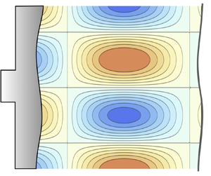
Pressure field in the compressed gas for ${\mathcal {R}}=6$, ${\mathcal {M}}_2=0.378$ and $h=0.7$ ($h>h_{c2}$) for two different boundary conditions corresponding to (a,c) piston-driven planar shock and (b,d) isolated shock. Panels (a,b) show the spatial pressure distribution at different times (solid lines) along with the shock pressure history (dashed lines).

The computations in figure 10, which have been also contrasted with the numerical integration of the Euler equations, have been done with ${\mathcal {R}}=6$, ${\mathcal {M}}_2=0.378$ and $h=0.7$ ($h>h_{c2}$) for two different boundary conditions corresponding to (a) a piston-driven planar shock and (b) an isolated shock. The upper plots show the spatial pressure distribution at different times (solid lines) together with the history of the pressure values at the shock along the spatial coordinate representing the shock position (dashed lines). The lower panels show the two-dimensional pressure field at $\tau =29$. It is found that the spatial frequency of the pressure field is much smaller than the frequency associated with the shock oscillations, as derived previously in (4.20a,b). Note that, unlike the case of the self-similar accretion shock discussed in Huete et al. (Reference Huete, Velikovich, Martínez-Ruiz and Calvo-Rivera2021) (see figure 11(a,c) there), the planar shock does not render a standing wave configuration downstream because the associated acoustic frequency $\omega _a$, see (4.20a,b), does not admit a null solution: $\omega _a>0$ for any value of the shock oscillation frequency.

4.2.3. The early-time behaviour

From the definition given in (3.4a,b), it is readily seen that when $h>1$, the sonic reflection coefficient $\mathscr {R}_s$ exceeds 1. It implies that the amplitude of the sonic wave normally incident at the shock is reflected back with a greater amplitude. Since the piston reflection coefficient is unity, it may be tempting to assume that the positive feedback accumulation should lead to unstable behaviour of the shock front ripple and associated perturbation variables. This is actually true for one-dimensional planar shocks, i.e. independent of the transverse coordinate, perturbations of planar shocks (Fowles & Swan Reference Fowles and Swan1973; Swan & Fowles Reference Swan and Fowles1975; Kuznetsov Reference Kuznetsov1984), as well as for acoustic radial perturbations in spherically and cylindrically expanding steady accretion shocks (Huete et al. Reference Huete, Velikovich, Martínez-Ruiz and Calvo-Rivera2021). In the former case, the one-dimensional nature of perturbations implies normal incidence for all reflections of a reverberating sonic wave. In the latter case, the near-normal incidence is ensured by the scale-free geometry of the perturbation field. In Appendix B the conclusion made first by Fowles & Swan (Reference Fowles and Swan1973) (see their figures 3 and 4) that one-dimensional perturbed planar shocks are actually unstable for $h>1$ is confirmed both numerically and theoretically, the power-law growth is established and the corresponding power index is calculated.

For two-dimensional planar shocks, both Laplace-transform analysis and numerical integration of Euler equations predict no change in the character of the solution, implying the absence of unstable behaviour when $h>1$. To illustrate the qualitative difference between perturbations in one and two dimensions, we utilise a Taylor expansion analysis that departs from the one-dimensional solution discussed previously by Fowles & Swan (Reference Fowles and Swan1973) and Kuznetsov (Reference Kuznetsov1984). This one-dimensional solution is a representative case when the shock–piston distance is much smaller than the perturbation wavelength. The Taylor expansion method accounts for deviations from the one-dimensional solution at later times that arise due to two-dimensional effects (as depicted in the sketch in figure 11).

Figure 11.

Sketch of the quasi-one-dimensional acoustic flow in the early time shock–piston reflection.

We seek the perturbed pressure in the form

(4.40)\begin{equation} \bar{p}(\eta,\tau)= \tau^{\sigma}\sum_{j=0}^\infty \phi_j(\eta) \tau^{2j}= \tau^{\sigma}\phi_0(\eta)+\tau^{\sigma}\sum_{j=1}^\infty \phi_j(\eta) \tau^{2j}, \end{equation}

where $\sigma$ is an eigenvalue to be determined. Such a form of solution, derived in Appendix B, stems from the fact that our perturbation problem is singular. In our small-amplitude approximation, we assume the shock-front ripple amplitude to be much smaller than all the characteristic lengths, including the shock–piston distance, but at $\tau \rightarrow 0$ the latter assumption is apparently violated. Further details can be found in §§ III.A and B of Velikovich (Reference Velikovich1996). It can be found there that the discrete spectrum of eigenvalues for a rigid piston is

(4.41)\begin{equation} \sigma = \begin{cases} 1 & \\ \dfrac{\ln \mathscr{R}_s}{\ln \mathscr{D}_s} + {\rm i}\dfrac{2 n {\rm \pi}}{\ln \mathscr{D}_s} , n=0,\pm 1, \pm 2,\ldots, \end{cases} \end{equation}

where $\sigma =1$ corresponds to the solution addressed before through the Laplace transform. It is also the solution considered by all previous authors, starting from Roberts (Reference Roberts1945). This eigenvalue exists independently of the EoS and shock parameters. For the ideal gas EoS used by these authors, the solution (4.40) with $\sigma =1$ is the only one that is finite in the limit $\tau \rightarrow 0$, which is the heuristic reason why all the other eigenmodes could be discarded. The early-time behaviour of this eigenmode can be characterised by the expression ${\bar p}_s= b_0 \tau + O(\tau ^3)$, where $b_0$ is defined in (3.5). In addition, we have $\xi _s= 1 + O(\tau ^2)$, indicating that the shock front maintains the initial shape of the rippled piston up to terms on the order of $\tau \sim 1$.

The discrete spectrum of $\sigma$ is given by the bottom-line expression in (4.41), which coincides with that obtained for the one-dimensional perturbed planar shock and presented in (B5a,b). It demonstrates that for $h>1$, implying $\mathscr {R}_s>1$, the real parts of all eigenvalues are positive, $\sigma _{R}>0$. Hence, the corresponding eigenmodes in (4.40) all vanish in the limit $\tau \rightarrow 0$. Since they are no longer singular, they cannot be discarded and must be included in our analysis. Unlike the one-dimensional planar case, which lacks proper scales, we utilise the previously defined dimensionless coordinates $\tau =kc_2 t$ and $\bar {x}=k x$ to construct the self-similar variable $\eta = \bar {x}/\tau$. Introducing this form of pressure perturbations into the sonic wave equation gives

(4.42)$$\begin{gather} \sigma(\sigma-1)\phi_0-2\eta(\sigma-1)\dfrac{{\rm d}\phi_0}{{\rm d}\eta}-(1-\eta^2)\dfrac{{\rm d}^2\phi_0}{{\rm d}\eta^2}\nonumber\\ +\displaystyle{\sum_{j=1}^\infty}\left[(2j+\sigma)(2j+\sigma-1)\phi_j-2\eta(2j+\sigma-1)\dfrac{{\rm d}\phi_j}{{\rm d}\eta}-(1-\eta^2)\dfrac{{\rm d}^2\phi_j}{{\rm d}\eta^2}+\phi_{j-1}\right]\tau^{2j}=0. \end{gather}$$

Likewise, the shock and piston boundary conditions can be expressed in terms of the eigenfunctions as

(4.43)\begin{align} &\left.\dfrac{1-h+2{\mathcal{M}}_2^2}{2{\mathcal{M}}_2}\sigma \phi_0({\mathcal{M}}_2)+(1-{\mathcal{M}}_2^2)\frac{{\rm d}\phi_0}{{\rm d} \eta}\right|_{\eta={\mathcal{M}}_2}\nonumber\\ &\quad +\sum_{j=1}^\infty\left\{\left[\dfrac{1-h+2{\mathcal{M}}_2^2}{2{\mathcal{M}}_2}(2j+\sigma) \phi_j({\mathcal{M}}_2)+\left.(1-{\mathcal{M}}_2^2)\frac{{\rm d}\phi_j}{{\rm d} \eta}\right|_{\eta={\mathcal{M}}_2}\right](2j+\sigma-1)\right.\nonumber\\ &\quad \left.+\dfrac{{\mathcal{M}}_2{\mathcal{R}}(1+h)}{2}\phi_{j-1}({\mathcal{M}}_2)\vphantom{\sum_{j=1}^\infty}\right\}\tau^{2j}=0 \end{align}

and ${\rm d}\phi _j/({\rm d} \eta )|_{\eta =0}=0$, respectively. Note that the solution of $\phi _0(\eta )$ corresponds to the purely one-dimensional perturbations described by (B12), with the eigenvalue being determined by $\mathscr {D}_s^{\sigma }=\mathscr {R}_s$, where $\mathscr {R}_s$ denotes the shock reflection coefficient defined in (3.4a,b) and $\mathscr {D}_s$ is the Doppler shift factor provided in (4.32). It describes the effectively planar sonic reflections when the shock is very close to the piston $\tau \ll 1$ and two-dimensional effects have not yet entered into play. The other eigenfunctions corresponding to $j>1$ can be recursively determined by

(4.44)\begin{equation} (2j+\sigma)(2j+\sigma-1)\phi_j-2\eta(2j+\sigma-1)\dfrac{{\rm d}\phi_j}{{\rm d}\eta}-(1-\eta^2)\dfrac{{\rm d}^2\phi_j}{{\rm d}\eta^2}={-}\phi_{j-1} , \end{equation}

subject to

(4.45)\begin{gather} \left.\dfrac{1-h+2{\mathcal{M}}_2^2}{2{\mathcal{M}}_2}(2j+\sigma) \phi_j({\mathcal{M}}_2)+(1-{\mathcal{M}}_2^2)\frac{{\rm d}\phi_j}{{\rm d} \eta}\right|_{\eta={\mathcal{M}}_2} ={-}\dfrac{{\mathcal{M}}_2{\mathcal{R}}(1+h)}{2 (2j+\sigma-1)}\phi_{j-1}({\mathcal{M}}_2), \end{gather}

(4.46)\begin{gather} \dfrac{{\rm d}\phi_j}{{\rm d} \eta}\bigg|_{\eta=0}=0. \end{gather}

Note that the inhomogeneous terms in (4.44) and (4.45), which involve the term $\phi _{j-1}$ (or $\phi _0(\eta )$ for $j=1$), account for the multidimensional character of the problem. For example, the factor proportional to $\phi _{j-1}({\mathcal {M}}_2)$ in (4.45) comes from direct combination of the shock ripple perturbation (2.6a) and tangential velocity conservation across the shock (2.6c), while the term $\phi _{j-1}(\eta )$ in (4.44) comes from the $\partial ^2p/(\partial y^2)$ in the sound wave equation.

The solution of our linear problem is presented as an infinite sum of these eigenfunctions with constant coefficients. When $\tau \ll 1$, i.e. when the distance of the shock from the piston is much smaller than the perturbation wavelength, the solution of this problem is the same as that for planar shock, where the eigenvalue $\sigma$ is determined by (B5a,b). Except for geometry factors, this is equivalent to the eigenvalue that characterises the cylindrical and spherical accretion shocks in the radial limit, see (3.3a) and (3.3b) in Huete et al. (Reference Huete, Velikovich, Martínez-Ruiz and Calvo-Rivera2021). However, in this case, the value of $\sigma$ is analytical, as opposed to the eigenfunction, which must be solved numerically for each mode number $n$ involved in $\sigma _{I}$. In the present case, the solution has been obtained iteratively by considering increasing values of $j$, starting from the one-dimensional solution for $j=0$ and using the given eigenmode $\sigma$. The numerical computation is rather demanding since the values of $\phi _j({\mathcal {M}}_2)$ must be calculated with high accuracy to capture the leading contributing terms for $\phi _j \tau ^{2 n}=O(1)$. For example, the solution of (4.44) and (4.45) is displayed in figure 12 for ${\mathcal {R}}=3$, ${\mathcal {M}}_2=1/2$ (which results in $h_c=0$) and $h=1.1$.

Figure 12.

Solution of (4.40) for $\eta ={\mathcal {M}}_2$ with the coefficients computed with (4.44) and (4.45) for (a) $\sigma =0.1826$ and (b) $\sigma =1$. Shock conditions: ${\mathcal {R}}=3$, ${\mathcal {M}}_2=1/2$ and $h=1.1$.

As a check of consistency, we can first evaluate the solution obtained by Taylor expansions with $\sigma =1$ and compare it with a previously validated solution, such as that obtained using the Bessel series method. This comparison is displayed in figure 12(b), which shows the solution obtained for the same shock parameters: ${\mathcal {R}}=3$, ${\mathcal {M}}_2=1/2$ and $h=1.1$. The Taylor-expansion solution rendered by (4.40) (represented in solid line) is initiated with the eigenfunction $\phi _0=b_0$ that is consistent with the $\sigma =1$ solution for $\tau \rightarrow 0$. The solution via Bessel series (circles) is computed in a similar form as done in figure 9. We observe that there is a perfect agreement between the two methods, which validates the use of (4.40) for computing the shock dynamics even for $h>1$. However, the major advantage of this approach is that it allows the investigation of the full set of eigenvalues, including those that lead to unstable behaviour in purely one-dimensional configurations. For example, figure 12(a) displays the case $\sigma _{R}=0.1826>0$ that results from the same shock conditions as those in figure 12(b) but obtained from (4.41) (bottom-line expression). The solution, which has been computed for $n=\sigma _{I}=0$ and with an arbitrary constant $C_0=1$ in (B12), has demanded 270 figures of accuracy to get the $j_{max}=45$ term, which is enough to capture the evolution of the shock pressure up to $\tau \sim 20$. A longer time solution could not be shown due to numerical limitations. The impact of the two-dimensional effects is readily seen. While the one-dimensional solution exhibits a positive power-law growth, the introduction of two-dimensional terms leads to a function with non-increasing amplitude oscillations. However, since we are also interested in the late-time asymptotic of our solutions, a legitimate question is: Is the decay slower than the powers of time $-3/2$ and $-1/2$ predicted by the classics for moderate-strength and strong shocks, respectively, in ideal gases? Regardless the case, it is the non-decaying contribution associated with the eigenvalue $\sigma =1$ that would dominate in the long-time regime.

For the piston-driven two-dimensional corrugated shock, the early time and the long-time behaviour are unrelated because we can unequivocally define the regimes with the aid of the temporal scale $1/(k c_2)$. On the other hand, scale-free perturbations follow the same power-law decay or growth throughout their evolution, from the early to the late time. This is true for one-dimensional perturbations in planar geometry, see Appendix B, and for all stable and unstable modes in spherical and cylindrical geometry (Huete et al. Reference Huete, Velikovich, Martínez-Ruiz and Calvo-Rivera2021). A heuristic argument can be made that their late-time asymptotics are the same as for the regular mode. It is based on the observation that each of the reverberation eigenmodes maintains a quasi-classical wave pattern, with a constant number of peaks and valleys between the shock and the piston, tracking the longitudinal mode number. The effective longitudinal wavelength increases as $t$, with the corresponding longitudinal wavenumber decreasing as $k_\parallel \sim 1/t$, whereas the transverse wavenumber $k_\perp =k$ remains constant. Hence, the reverberating sonic waves evolve to a grazing incidence, effectively decoupling the shock from the piston, irrespective of the value of the reflection coefficient $\mathscr {R}_s$ for normal incidence. The above explanation is consistent with the way the situation changes when the piston oscillates addressed in § 5: then the numbers of added peaks and values increase linearly with time, so $k_\parallel$ does not tend to zero, maintaining a finite angle of incidence of the reverberating sonic waves, leading to a non-resonant increase in the shock ripple amplitude with time.

We have commented previously that the particular case $h=h_m=1+2 {\mathcal {M}}_2^2$ renders an infinite initial slope for the pressure evolution, as seen in (3.5). This stems from the fact that the sonic reflection coefficient for normal incidence $\mathscr {R}_s=\mathscr {D}_s$. In other words, the Doppler-shift weakening of a sonic wave in a single cycle of its reverberation between the shock and the piston, $1/\mathscr {D}_s$, is exactly compensated for by its amplification in the shock reflection, because $\mathscr {R}_s>1$. Then, in this case the eigenvalue becomes degenerate because both top line and bottom line of (4.41) yields the same value $\sigma =1$. Then, the corresponding time dependence for the shock ripple takes the form $\xi _s\sim \ln \tau$, which diverges for $\tau \rightarrow 0$.