





1. Introduction
Taylor–Aris dispersion refers generally to the enhanced broadening of a solute plug when subjected to flow in a channel. G.I. Taylor (Reference Taylor1953) first developed an analytical model to analyse this dispersion, reporting a solution for the asymptotic (long-time) behaviour of solute subject to Poiseuille flow in a cylindrical tube. Taylor assumed that the effects of axial molecular diffusion were negligible compared with the overall dispersion and that the concentration of solute was nearly uniform across the channel cross-section. In such a regime, the effects of radial diffusion approximately balance with the non-uniform advective dispersion. This causes the full, three-dimensional (3-D) convection–diffusion equation to collapse to a linear one-dimensional (1-D) partial differential equation (PDE) for the area-averaged concentration, which predicts that the solute zone forms an axial Gaussian distribution in the long-time limit. Taylor’s solution is applicable in a regime which can be summarised as
 $6.9 \ll {\textit{Pe}} \ll L/a$
. Here,
 ${\textit{Pe}}$
is a Péclet number based on the inner radius of the tube,
 $a$
, and
 $L$
is a characteristic channel length. Aris (Reference Aris1956) soon generalised Taylor’s analysis to include the effects of axial molecular diffusion by introducing the so-called method of moments (MoM). The MoM generates one PDE and one ordinary differential equation (ODE) governing each axial moment of the solute zone (e.g. the mean axial position and axial solute variance) by integrations of the convection–diffusion equation. Importantly, the MoM allows for dispersion analysis at time scales earlier than Taylor’s method. Overall, Taylor–Aris dispersion is of fundamental importance to a diverse array of physical systems, such as chemical separation systems, microfluidic chips and environmental flows (Brenner & Edwards Reference Brenner and Edwards1993).
Since these seminal works, alternative models have been proposed to extend Taylor–Aris analyses to a wide variety of applications. Most frameworks expand the concentration field into (different types of) infinite series, then truncate these series after their first few terms. For example, the work of Gill (Reference Gill1967), later formalised by Gill & Sankarasubramanian (Reference Gill and Sankarasubramanian1970, Reference Gill and Sankarasubramanian1971), postulates that the solute concentration field can be written as an infinite series of the axial derivatives of the area-averaged concentration field. This is known as a Kramers–Moyal-type expansion. The dispersion coefficients, which act as eigenvalues of this ansatz, correspond to the integral moments of the solute zone. This solution method is represented in the works of Degance & Johns (Reference Degance and Johns1978a , Reference Degance and Johns b ), Mauri (Reference Mauri1991), Paul & Ng (Reference Paul and Ng2012) and Wang & Chen (Reference Wang and Chen2016). A related method is that of Edgeworth expansions, introduced by Chatwin (Reference Chatwin1970, Reference Chatwin1972). This model extends the original MoM by expanding the concentration field into an Edgeworth–Cramér series to more accurately model the area-averaged concentration distribution. Guan & Chen (Reference Guan and Chen2024) later advanced this solution method to model the 3-D concentration field in pipe Poiseuille flow. Another extension of the original MoM came from Barton (Reference Barton1983), who applied the MoM to channels of arbitrary (but uniform) cross-section and arbitrary steady, parallel flows. The Aris–Barton MoM is applied or extended by Bandyopadhyay & Mazumder (Reference Bandyopadhyay and Mazumder1999), Vedel & Bruus (Reference Vedel and Bruus2012) and Samuel et al. (Reference Samuel, Chang, Ma and Santiago2025). The main advantage of these series-based methods over Taylor’s original method is that, in theory, these models are applicable at all time scales. However, these models usually become intractable past the third or fourth terms. We note that the solute zone is typically not well described by its first few integral moments at early times for inhomogeneous initial conditions (Frankel & Brenner Reference Frankel and Brenner1989).
Perhaps the most significant generalisation of Taylor–Aris dispersion is the so-called generalised Taylor dispersion theory or macrotransport paradigm, which originated primarily from Howard Brenner and his collaborators (Brenner Reference Brenner1980b
, Reference Brenner1982a
,
Reference Brennerb
; Dill & Brenner Reference Dill and Brenner1982a
, Reference Dill and Brenner
b
; Frankel & Brenner Reference Frankel and Brenner1989; Brenner & Edwards Reference Brenner and Edwards1993). Generalised Taylor dispersion theory solves the convection–diffusion equation in a phase space
 $\unicode{x1D64C} \oplus\unicode{x1D666}$
, where
 $\unicode{x1D64C}$
is a ‘global’ unbounded subspace and
 $\unicode{x1D666}$
is a ‘local’ bounded subspace. For example,
 $\unicode{x1D64C}$
may represent the axial position of solute in a tube or the lattice position in an infinite array. The coordinates
 $\unicode{x1D666}$
may represent the location of solute in the tube cross-section, the orientation of a non-spherical Brownian particle of finite size or the axial position of solute within an individual unit cell in porous media. Elliptic boundary-value problems in the ‘local’ coordinates must first be solved to find the steady-state probability density function of solute within the local coordinates, as well as the so-called
 $\unicode{x1D63D}$
field (Frankel & Brenner Reference Frankel and Brenner1989). These quantities are then used to compute
 $m$
-adic transport tensors (for example, the dispersion dyadic), which enable reconstruction of the solute behaviour in the long-time limit via the Fourier transform. Because of the generality of the ‘local’ subspace, the macrotransport paradigm has been successfully applied to a wide variety of transport problems. These include, for example, dispersion in porous media (Brenner Reference Brenner1980a
; Brenner & Adler Reference Brenner and Adler1982; Dill & Brenner Reference Dill and Brenner1983; Salles et al. Reference Salles, Thovert, Delannay, Prevors, Auriault and Adler1993), dispersion involving non-spherical or finite-sized particles (Brenner Reference Brenner1981; Mavrovouniotis & Brenner Reference Mavrovouniotis and Brenner1988), dispersion of chemically reactive species (Shapiro & Brenner Reference Shapiro and Brenner1986, Reference Shapiro and Brenner1987, Reference Shapiro and Brenner1988) and dispersion of active swimmers (Manela & Frankel Reference Manela and Frankel2003; Wang et al. Reference Wang, Jiang, Zeng, Wu and Wang2025). Generalised Taylor dispersion theory is also highly applicable to analysing spatially periodic systems. Examples include dispersion in periodic channels of slowly varying radius (or channel height) in both pressure-driven flow (Hoagland & Prud’Homme Reference Hoagland and Prud’Homme1985; Bolster et al. Reference Bolster, Dentz and Le Borgne2009; Dorfman Reference Dorfman2009) and low-zeta potential electro-osmotic flow (Yariv & Dorfman Reference Yariv and Dorfman2007; Dorfman Reference Dorfman2008).
Significant work has been dedicated towards analysing dispersion in non-spatially periodic systems. One method to study channels with axially varying flow properties is centre manifold theory, pioneered by Mercer & Roberts (Reference Mercer and Roberts1990, Reference Mercer and Roberts1994). Mercer & Roberts applied centre manifold theory to dispersion in Poiseuille flow in both a 1-D channel with slow axial variations in height and an axisymmetric tube with slow axial variations in radius. In addition to centre manifold theory, the original area-averaging method of Taylor is also applicable to study dispersion in channels with streamwise variations in flow properties. Horner et al. (Reference Horner, Arce and Locke1995) applied this area-averaging method to conical channels with converging and diverging sections. Stone & Brenner (Reference Stone and Brenner1999) soon formalised this area-averaging approach and used this technique to study dispersion in radially expanding flow between two parallel plates. This geometry results in flow with streamwise variations in mean velocity and, thus, also is an example of a non-periodic system. More recently, Chang & Santiago (Reference Chang and Santiago2023) used an area-averaging method to study dispersion in Poiseuille flow in axisymmetric channels with slowly varying radii. They derived two coupled ODEs for the mean axial position of solute and axial solute variance. This enables analysis of both the short- and long-term spatial solute evolution. Importantly, Chang & Santiago also developed an approach to engineer channels to yield particular spatial solute variance distributions by solving a nonlinear, first-order ODE. Using the latter methodology, Teodoro et al. (Reference Teodoro, Bautista and Méndez2025) analysed the dispersion in pressure-driven flow of viscoelastic fluids in axisymmetric channels with varying radii.
Overall, previous studies of Taylor dispersion in channels have focused on periodic geometries, 1-D flow fields and/or axisymmetric systems. Additionally, studies that follow the macrotransport paradigm are restricted to periodic channels and asymptotically long times (Brenner & Edwards Reference Brenner and Edwards1993). In contrast, studies that do not follow the macrotransport paradigm typically rely on scaling analyses tailored to one geometry and velocity field. Moreover, most previous works (excluding Chang & Santiago Reference Chang and Santiago2023) provide only limited engineering insight for the design of channels that produce specified solute distributions. To our knowledge, no prior model captures dispersion in channels with arbitrary, slowly varying cross-sectional shape and size.
In this work, we present a reduced-order framework for the analysis of dispersion in long, straight channels whose cross-sections vary slowly but arbitrarily. These variations in cross-section can include changes in shape, size or both. We consider arbitrary flow fields (which may vary slowly in time), such as pressure-driven, electro-osmotic and free-surface flow (or combinations thereof). We follow an area-averaging approach, which leads to the introduction of a new ‘solute deviation source field’, here termed
 $\varPsi$
. This field is determined by the solution of a Poisson equation in the channel cross-section with a source determined by axial velocity deviations and the local relative rate of change of cross-section area. We show this
 $\varPsi$
field closes the dispersion problem and enables us to derive a 1-D PDE for the development of the area-averaged solute concentration. Concurrently, we develop expressions to reconstruct the full, 3-D concentration field. In the regime where the solute cloud is localised relative to variations in the channel geometry, we formulate two simple coupled ODEs for the mean axial position and axial variance of solute. We further derive an ODE that can be used to engineer channel geometries that produce specified axial variance patterns for a given flow field (which we refer to as the inverse problem). We apply and demonstrate our theory to three very different channel geometries and benchmark our results against Brownian dynamics simulations. These three geometries are axisymmetric tubes with varying radii, channels with a roughly ‘dumbbell-shaped’ cross-section that varies along the flow direction, and rectangular channels of varying aspect ratio and area.
2. Theory
2.1. Taylor-type analysis of solute dispersion
We analyse Taylor–Aris type dispersion (Taylor Reference Taylor1953; Aris Reference Aris1956) for a neutral (uncharged) solute subject to flow in a piecewise smooth 3-D channel. The channel cross-section in the spanwise-transverse plane, denoted by
 $S(x) \in \mathbb{R}^2$
, is assumed to be bounded and can vary slowly with respect to axial position,
 $x$
. Letting
 $\boldsymbol{u}(x, y, z, t) = (u, v, w)$
denote the flow field in the channel,
 $D$
represent the molecular diffusivity of the solute and
 $c(x, y, z, t)$
be the concentration of solute, the convection-diffusion equation can be expressed as
 \begin{align} \begin{aligned} \frac {\partial c}{\partial t} +\boldsymbol{u} \boldsymbol{\cdot }\boldsymbol{\nabla }c = D \big ({\nabla} ^2 c\big ) ; \boldsymbol{\nabla }c \boldsymbol{\cdot }\hat {\boldsymbol{n}} = 0. \end{aligned} \end{align}
Here,
 $\hat {\boldsymbol{n}} = (n_x, n_y, n_z)$
is the outward unit normal vector to the fluid domain. To derive expressions for the solute concentration, we will employ a general area-averaging and deviation method based on that of Stone & Brenner (Reference Stone and Brenner1999). We define a cross-sectional average as
 $\langle (.) \rangle :=({1}/{A(x)} )\int \kern-5pt \int _{S(x)}(.)\,{\textrm d}A$
, where
 $A(x) = \int \kern-5pt \int _{S(x)}\, {\textrm d}A$
, and the deviation from this average as
 $(.)' := (.) - \langle (.) \rangle$
. Expanding (2.1) into area averages and deviations,
 \begin{align} \begin{aligned} \frac {\partial \langle c \rangle }{\partial t} + \frac {\partial c'}{\partial t} +\langle \boldsymbol{u} \rangle \boldsymbol{\cdot }\boldsymbol{\nabla }c' + \boldsymbol{u}' \boldsymbol{\cdot }\boldsymbol{\nabla }c' + \langle u \rangle \frac {\partial \langle c \rangle } {\partial x} + u' \frac {\partial \langle c \rangle } {\partial x} = D \left ({\nabla} ^2 c' + \frac { \partial ^2 \langle c \rangle }{\partial x^2}\right )\!. \end{aligned} \end{align}
Taking an area average of (2.2),
 \begin{align} \begin{aligned} \frac {\partial \langle c \rangle }{\partial t} +\langle \boldsymbol{u} \rangle \boldsymbol{\cdot }\langle \boldsymbol{\nabla }c' \rangle + \langle \boldsymbol{u}' \boldsymbol{\cdot }\boldsymbol{\nabla }c' \rangle + \langle u \rangle \frac {\partial \langle c \rangle } {\partial x} = D \left (\bigl\langle{\nabla} ^2 c' \bigr\rangle + \frac { \partial ^2 \langle c \rangle }{\partial x^2}\right )\!. \end{aligned} \end{align}
 \begin{align} \frac {\partial c'}{\partial t} +\langle \boldsymbol{u} \rangle \boldsymbol{\cdot }\boldsymbol{\nabla }c' + \boldsymbol{u}' \boldsymbol{\cdot }\boldsymbol{\nabla }c' + u' \frac {\partial \langle c \rangle } {\partial x} - \langle \boldsymbol{u} \rangle \boldsymbol{\cdot }\langle \boldsymbol{\nabla }c' \rangle - \langle \boldsymbol{u}' \boldsymbol{\cdot }\boldsymbol{\nabla }c' \rangle = D \big ({\nabla} ^2 c' - \langle {\nabla} ^2 c' \rangle \big ). \end{align}
We now perform a scaling analysis of (2.4). There are two primary axial length scales of interest in this formulation: these are the characteristic width of the solute zone,
 $\sigma$
, and the characteristic length over which changes in the channel geometry occur,
 $\lambda$
. In the cross-sectional plane, there are three length scales of interest: the maximum physical extent of the channel in the spanwise direction (
 $y_0$
), the maximum physical extent of the channel in the transverse direction (
 $z_0$
) and a length scale derived from the maximum solute diffusion time,
 $t_{ {\textit{diff}}}$
, for two-dimensional (2-D) diffusion in the
 $y, z$
plane.
The time scale
 $t_{{\textit{diff}}}$
can be defined as the time required for Brownian diffusion to homogenise particles along the cross-section of a given channel. This time scale may be obtained from, for example, a separate analysis or simulation of 2-D diffusion along the cross-section of the channel. Given such an estimate, we define a relevant length scale as
 $a_0 = \sqrt {t_{{\textit{diff}}}D}$
. Note that, invariably,
 $y_0, z_0 \le a_0$
. Also, for channel cross-sections which have at least one highly constrained region (where two opposing walls are very near one another), we expect that
 $y_0, z_0 \ll a_0$
(e.g. as in the downstream shape of the channel shown in figure 1). We here hypothesise that for a length scale for the solute to homogenise along the cross-section of a channel, scaling
 $y$
and
 $z$
with
 $a_0$
(and importantly basing our smallness parameters on
 $a_0$
) is more meaningful than scaling with either
 $y_0$
or
 $z_0$
. However, non-dimensionalising
 $z$
and
 $y$
with the channel half-height and half-width is typically more straightforward, and indeed is often desirable when solving for the concentration field in a particular channel. The latter approach is valid so long as the necessary smallness parameters (cf. table 1) hold in terms of
 $a_0$
. Further, as discussed in § A of the supplementary material (SM) available at https://doi.org/10.1017/jfm.2026.11864, simple heuristic approximations for
 $a_0$
are often sufficient to perform a scaling analysis for most common channel geometries; hence, 2-D diffusion simulations may not always be necessary to find
 $a_0$
to the correct order-of-magnitude. In the latter section of the SM, we provide an example approximation of
 $a_0$
.
Summary of terms in (2.4) and of the assumptions made in this manuscript.

Table 1. Long description
An equation with assumptions and derivations for a mathematical model. The left-hand side of the equation includes terms with U C 0 over sigma, U C 0 times O of open parenthesis C 0 prime over C 0 close parenthesis, U C 0 over sigma times O of open parenthesis S T C 0 prime over C 0 close parenthesis, and U C 0 over sigma times O of open parenthesis gamma C 0 prime over C 0 close parenthesis. The right-hand side includes terms with D C 0 prime over a 0 squared times O of 1 and D C 0 prime over a 0 squared times O of H squared. Assumptions needed to derive the equation include eta being much less than 1, C 0 prime over C 0 being much less than 1, gamma C 0 prime over C 0 being much less than 1, eta P e being much less than 1, and S T C 0 prime over C 0 being much less than 1. Further assumptions include gamma being much less than 1 and the functions mu, Gamma, open parenthesis x minus x bar close parenthesis Gamma, A to the power of minus 1, x A to the power of minus 1, and Psi u prime being accurately approximated by Taylor series expansions about the mean axial position of solute.
Schematic of a solute zone of characteristic width
 $\sigma$
being transported through a long-thin tube under flow. The 3-D velocity field components are represented by the lime green arrows; the dotted black lines denote the coordinate system. The channel cross-section
 $S(x)$
, illustrated by the light blue regions, slowly varies in shape (and net size) along the axial direction,
 $x$
. The orange vector represents the outward unit normal vector to the fluid domain,
 $\hat {\boldsymbol{n}}$
. Both the characteristic spanwise width and transverse depth of the channel (respectively denoted by
 $y_0$
and
 $z_0$
) are depicted enlarged relative to the axial length of the channel for clarity of presentation.

Next, the remaining terms in (2.4) are non-dimensionalised as
 $c' = c_0^{\prime} c'^{*}$
,
 $\langle c \rangle = c_0 \langle c^{*} \rangle$
,
 $\boldsymbol{u} = (U u^{*}, V v^{*}, W w^{*})$
,
 $\boldsymbol{u}' = (U u'^{*}, V v'^{*}, W w'^{*})$
and
 $t = t_ct^{*}$
, where
 $t_c$
is some characteristic time scale of the flow (e.g. an advection time scale or the time scale of some forcing function of the flow). The incompressible continuity relation then suggests that
 $V \sim W \sim (a_0/\lambda ) U$
. For our scaling analysis, we assume the following main smallness parameters:
 $\eta = a_0 / \sigma \ll 1$
(long-thin channel),
 $c_0^{\prime}/c_0 \ll 1$
,
 $\eta {\textit{Pe}} = (U a_0^2)/(\sigma D) \ll 1$
(the solute diffusion time in the cross-section is small compared with the characteristic time scale of the flow) and
 $St(c'_0/c_0) \ll 1$
. Here,
 ${\textit{Pe}} = (a_0 U)/D$
is the flow Péclet number and
 $St = \sigma /(t_cU)$
is the Strouhal number. We note that for steady flows or flows with characteristically long time scales, the characteristic flow time scale relevant to dispersion becomes the advection time scale (i.e.
 $t_c = t_{adv} = \sigma / U$
) and the Strouhal number reduces to unity. In the latter cases, this constrains the Strouhal number from ever becoming significantly smaller than
 $1$
. Next, note that the assumption
 $\eta \ll 1$
combined with the fact that we work in constant, laboratory coordinates implicitly constrains the channel to be mostly straight. This is because we define
 $\sigma$
as the width of the solute cloud in the laboratory
 $x$
direction (not necessarily the channel centreline direction) and
 $a_0$
as the solute diffusion time in the
 $y, z$
plane (not necessarily the plane orthogonal to the channel centreline). Thus, if the channel takes e.g. a
 $90^\circ$
turn along the streamwise direction, the assumption
 $\eta \ll 1$
would be violated and the model would fail. Therefore, the channel must be mostly straight in the streamwise direction. We also note the classic Taylor hypothesis
 $c_0^{\prime} \ll c_0$
should hold so long as
 $t_{{\textit{diff}}}/t_{\textit{advection}} = \eta {\textit{Pe}} \ll 1$
. Lastly, we define the parameter
 $\gamma = \sigma /\lambda$
. To derive (2.16), we assume
 $\gamma (c'_0/c_0) \ll 1$
, which will certainly be satisfied if
 $\gamma \lesssim \mathcal{O}(1)$
(because we assume separately that
 $c'_0/c_0 \ll 1)$
. However, to derive simple approximate ODEs for the solute variance and to engineer channels for specific solute variance patterns, we shall later consider a regime where
 $\gamma \ll 1$
. Using the aforementioned scales and smallness parameters, we estimate the order-of-magnitude of each term in (2.4). For a detailed ranked summary of the orders of magnitudes of the terms in (2.4), see table 1. Keeping only terms of
 $\mathcal{O}(1)$
in (2.4) results in
 \begin{align} \begin{aligned} u' \frac {\partial \langle c \rangle } {\partial x} \approx D \left ( \frac { \partial ^2 c'}{\partial y^2} +\frac { \partial ^2 c'}{\partial z^2} - \left \langle \frac { \partial ^2 c'}{\partial y^2} + \frac { \partial ^2 c'}{\partial z^2}\right \rangle \right )\!. \end{aligned} \end{align}
Equation (2.5) demonstrates an approximate balance between the advective dispersion arising from the non-uniform axial velocity field and the cross-sectional diffusion, as well as an additional area-averaged term arising from changes in the channel geometry. The balance between cross-sectional diffusion and advective dispersion alone is a hallmark of Taylor dispersion theory for channels of uniform cross-section (Taylor Reference Taylor1953). To derive an expression for the tracer concentration, we first simplify the area-averaged term on the right-hand side of (2.5). Letting
 $\boldsymbol{\nabla} _{\perp }(.)$
refer to the gradient in the
 $y, z$
plane and
 $\hat {\boldsymbol{n}}_{\perp } = (n_y, n_z)$
, we expand the latter term as
 \begin{align} \begin{aligned} - D \left \langle \frac { \partial ^2 c'}{\partial y^2} + \frac { \partial ^2 c'}{\partial z^2}\right \rangle &= -\frac {D}{A(x)} \int\kern-5pt\int _{S(x)} \boldsymbol{\nabla} _{\perp } \boldsymbol{\cdot }(\boldsymbol{\nabla} _{\perp }c)\,{\textrm d}A \\ &= -\frac {D}{A(x)} \oint _{\partial S(x)} \frac {1}{\sqrt {n_y^2 + n_z^2}} (\boldsymbol{\nabla} _{\perp }c) \boldsymbol{\cdot }\hat {\boldsymbol{n}}_{\perp }\, {\textrm d}s \\ &= \frac {D}{A(x)} \oint _{\partial S(x)} \frac {1}{\sqrt {1-n_x^2}} \frac {\partial c}{\partial x} n_x \,{\textrm d}s, \end{aligned} \end{align}
where the third equality holds from the 3-D no-flux boundary condition. Note that under the assumption
 $n_x \sim a_0/\lambda \ll 1$
, the following prefactor from (2.6) is approximately unity:
 $(1-n_x^2)^{-1/2} = 1 + n_x^2/2 + \mathcal{O}(\eta ^4 \gamma ^4) \approx 1$
. Thus, we can write (2.6) as
 \begin{align} \frac {D}{A(x)} \oint _{\partial S(x)} \frac {1}{\sqrt {1-n_x^2}} \frac {\partial c}{\partial x} n_x\, {\textrm d}s &\approx \frac {D}{A(x)} \frac {\partial \langle c \rangle }{\partial x} \oint _{\partial S(x)} n_x\, {\textrm d}s +\frac {D}{A(x)} \oint _{\partial S(x)} \frac {\partial c'}{\partial x} n_x \,{\textrm d}s \notag\\ &\approx D \varGamma (x) \frac {\partial \langle c \rangle }{\partial x}. \end{align}
Here,
 \begin{align} \begin{aligned} \varGamma (x) = \frac {1}{A(x)}\left (\oint _{\partial S(x)} n_x\, {\textrm d}s \right ) \approx - \frac {1}{A(x)} \frac {{\textrm d}A(x)}{{\textrm d}x} + \mathcal{O} (\gamma ^2 \eta ^2) \end{aligned} \end{align}
is a function describing the local tube geometry (see Appendix A for proof of the second identity in (2.8)). Also, the term
 $(D \oint _{\partial S(x)} (\partial c' /\partial x) n_x \,{\textrm d}s)/A(x)$
in (2.7) is of magnitude
 $(D c_0/a_0^2)\mathcal{O}(\gamma \eta ^2 c_0^{\prime}/c_0)$
and so has been neglected. Substituting (2.7) into (2.5), we arrive at
 \begin{align} \begin{aligned} u' \frac {\partial \langle c \rangle } {\partial x} \approx D \left ({\nabla} ^2_{\perp } c' +\varGamma (x) \frac {\partial \langle c \rangle }{\partial x} \right )\!, \end{aligned} \end{align}
which is a much more manageable expression than (2.5).
Proceeding with the derivation, first note that if we can find an expression for the deviation variable
 $c'$
in terms of
 $ \partial \langle c \rangle /\partial x$
, we can close (2.3). To achieve this goal, we first rearrange (2.9) as
 \begin{align} \begin{aligned} {\nabla} ^2_{\perp } c' = \left (\frac {u'}{D} - \varGamma (x)\right )\frac {\partial \langle c \rangle }{\partial x} ; \quad\boldsymbol{\nabla} _{\perp } c' \boldsymbol{\cdot }\hat {\boldsymbol{n}}_{\perp } = -\frac {\partial \langle c \rangle }{\partial x} n_x. \end{aligned} \end{align}
Note that the term
 $(\partial c'/\partial x)n_x$
in the boundary condition on (2.10) is of
 $\mathcal{O}(\gamma \eta ^2)$
and so has been neglected. Any solution to (2.10) will be of the form
 \begin{align} \begin{aligned} c'(x, y, z, t) = \varPsi \frac {\partial \langle c \rangle }{\partial x} , \end{aligned} \end{align}
where, for all
 $x$
,
 $\varPsi$
satisfies
 \begin{align} \begin{aligned} {\nabla} ^2_{\perp } \varPsi = \frac {u'}{D} - \varGamma (x);\quad \boldsymbol{\nabla} _{\perp } \varPsi \boldsymbol{\cdot }\hat {\boldsymbol{n}}_{\perp } = -n_x. \end{aligned} \end{align}
From the definition (2.11),
 $\varPsi$
can be understood as a field which quantifies local deviations from the area-averaged solute concentration. In regions where
 $\varPsi$
is large, non-uniform advection dominates over molecular diffusivity (cf. (2.12)), which creates regions of local solute inhomogeneity. We therefore term
 $\varPsi$
the ‘solute deviation source field’. Moreover, these deviations in concentration increase local dispersion, which is the Taylor dispersion effect. Next, from the definition
 $\varGamma (x) = (\oint _{\partial S(x)} n_x\, {\textrm d}s)/A(x)$
, the Fredholm solvability condition
 \begin{align} \begin{aligned} \int \kern-5pt \int _{S(x)} \left (\frac {u'}{D} - \varGamma (x)\right )\, {\textrm d}A = - \varGamma (x) A(x) = - \oint _{\partial S(x)} n_x\, {\textrm d}s \end{aligned} \end{align}
on (2.12) holds vacuously (Evans Reference Evans2010, ch. 6). The latter fact combined with the identity
 $\langle \varPsi \rangle = 0$
(cf. (2.11)) shows that at each point
 $x$
, a unique local
 $\varPsi$
field will exist for a given piecewise smooth channel and flow. Furthermore, (2.11) reveals that the global
 $\varPsi$
field (defined as the unique field that solves (2.12) at each point
 $x$
) will be smooth for any time
 $t\gt 0$
. Additionally, the
 $\varPsi$
field can be decomposed into a subfield arising from variations in the channel geometry and a subfield arising from the non-uniform axial velocity field, both of which still satisfy Fredholm solvability conditions. These subfields are
 \begin{align} \begin{aligned} {\nabla} ^2_{\perp } \varPsi _{ {\textit{velo}}} = \frac {u'}{D}; \quad \boldsymbol{\nabla} _{\perp } \varPsi _{{\textit{velo}}} \boldsymbol{\cdot }\hat {\boldsymbol{n}}_{\perp } = 0, \end{aligned} \end{align}
and
 \begin{align} \begin{aligned} {\nabla} ^2_{\perp } \varPsi _{ {\textit{geo}}} = - \varGamma (x);\quad \boldsymbol{\nabla} _{\perp } \varPsi _{ {\textit{geo}}} \boldsymbol{\cdot }\hat {\boldsymbol{n}}_{\perp } = -n_x, \end{aligned} \end{align}
so that
 $\varPsi = \varPsi _{ {\textit{velo}}} + \varPsi _{ {\textit{geo}}}$
. Decomposing
 $\varPsi$
into velocity- and geometry-based components is not necessary, but can often make solving for dispersion in complicated velocity fields and geometries more straightforward. We further note that in geometries of a uniform cross-section,
 $\varPsi _{ {\textit{geo}}}$
reduces to identically zero (a fact that follows from Green’s first identity). Next, (2.12) implies that
 $\varPsi \sim a_0 ({\textit{Pe}} + \eta \gamma ) \sim a_0 \max ({\textit{Pe}}, \eta \gamma )$
. Further, because
 $\varPsi$
is a function of the tube geometry (cf. (2.12)), note that
 $\partial \varPsi /\partial x \sim (a_0/\lambda ) \max ({\textit{Pe}}, \eta \gamma )$
. Another useful identity is
 $\langle {\nabla} _{\perp }^2 \varPsi \rangle = - \varGamma (x)$
.
The deviation generating function
 $\varPsi$
provides a relationship between
 $c'$
and
 $\partial \langle c \rangle /\partial x$
. As previously mentioned, the
 $\varPsi$
field therefore allows us to close (2.3) by substituting the definition of
 $\varPsi$
from (2.11) into (2.3), which yields
 \begin{align} \frac {\partial \langle c \rangle }{\partial t} + \left ( \langle u \rangle + \langle \boldsymbol{u} \rangle \boldsymbol{\cdot }\langle \boldsymbol{\nabla }\varPsi \rangle + \langle \boldsymbol{u}' \boldsymbol{\cdot }\boldsymbol{\nabla }\varPsi \rangle + D \varGamma (x) - D \left \langle \frac {\partial ^2 \varPsi }{\partial x^2} \right \rangle \right ) \frac {\partial \langle c \rangle }{\partial x} \notag\\\quad = D \left (1 + 2 \left \langle \frac {\partial \varPsi }{\partial x} \right \rangle - \frac { \langle \varPsi u' \rangle }{D} \right ) \frac {\partial ^2 \langle c \rangle }{\partial x^2}. \end{align}
Equation (2.16) is a powerful framework to simplify dispersion even in highly complex channels and flow fields. Note that the
 $\varPsi$
field closes the dispersion problem and yields a 1-D reduced-order model that accurately describes the essential physics of the 3-D solute distribution. The leading-order advective dispersion is captured through the term
 $\langle \varPsi u' \rangle /D$
, which can be interpreted as the cross-correlation between the solute deviation source field and deviations in the axial flow velocity. The term
 $D \varGamma (x)$
characterises leading-order perturbations of the solute centre-of-mass velocity arising from variations in the channel geometry. Equation (2.16) can typically be solved analytically for channel cross-sections that admit a separation of variables (e.g. see § 3.1). However, numerical solutions are often required to evaluate
 $\varPsi$
for complicated geometries and flow fields. Nonetheless, as a 1-D equation, (2.16) is far more tractable than solving the full, 3-D convection–diffusion equation. A general procedure for solving (2.16) is outlined as follows. To begin, the geometry of the tube must be specified, which allows direct calculation of
 $\varGamma$
from the definition (2.8). The
 $\varPsi _{ {\textit{geo}}}$
field can then be found by solving (2.15). To continue further, a velocity field and molecular diffusivity must be specified. Once the latter quantities are known, computing a solution to (2.14) gives
 $\varPsi _{{\textit{velo}}}$
. The full
 $\varPsi$
field is then simply
 $\varPsi = \varPsi _{ {\textit{velo}}} + \varPsi _{ {\textit{geo}}}$
. After finding gradients in the
 $\varPsi$
field, (2.16) is readily solvable to determine the area-average solute concentration. From here, the relationship (2.11) yields the deviation from the area-averaged concentration field. In this way, an expression for the full, 3-D solute concentration field can be found in a direct, systematic manner. We will perform such a derivation of the 3-D, unsteady concentration field in § 3.
Importantly, (2.16) was derived without assuming that
 $\gamma \ll 1$
; thus, (2.16) is applicable across a wide variety of Péclet numbers and flow conditions. As such, we will solve (2.16) for Péclet numbers of 10, 100 and 1000 for the special case of an axisymmetric channel in § 3.1. We will also solve (2.16) in a channel whose cross-section is shaped like a varying (along streamwise direction) dumbbell in § 3.2.
In the next section, we will consider solutions under the assumption
 $\gamma \ll 1$
. This limiting case is applicable to a significant subset of dispersion conditions and this assumption will allow us to derive simple ODEs for the integral moments of the solute distribution. This assumption will also allow us to engineer channels to create specific solute variance patterns.
2.2. Further simplifications for the long-wavelength regime for
 $\gamma \ll 1$

In the limit
 $\gamma \ll 1$
, several terms in (2.16) become negligibly small. Table 2 offers a detailed summary of the orders of magnitudes of the terms in (2.16). We keep the
 $\mathcal{O}({\textit{Pe}}^2)$
,
 $\mathcal{O}(1)$
,
 $\mathcal{O}(St)$
and
 $\mathcal{O}(\eta \gamma {\textit{Pe}}^{-1})$
terms (cf. table 2) in (2.16) and neglect higher-order terms, leading to
 \begin{align} \begin{aligned} \frac {\partial \langle c \rangle }{\partial t} + \left (\langle u \rangle + D \varGamma (x) \right ) \frac {\partial \langle c \rangle } {\partial x}= D \left (1 -\frac { \langle \varPsi u' \rangle }{D} \right )\frac {\partial ^2 \langle c \rangle }{\partial x^2}. \end{aligned} \end{align}
Equation (2.17) combined with (2.12) and the flow field form a closed system. The effective dispersion coefficient is given as
 \begin{align} \begin{aligned} D^{*}_{{\textit{eff}}}(x) = \left (1 -\frac { \langle \varPsi u' \rangle }{D} \right )\!. \end{aligned} \end{align}
Ranked summary of terms in (2.16).

Table 2. Long description
An equation with various terms ranked by their significance. The equation includes advective and diffusive terms, each with different orders of magnitude. The advective terms are ranked as follows: U C 0 over sigma times O of 1, U C 0 over sigma times O of S t, U C 0 over sigma times O of open parenthesis eta gamma close parenthesis squared times P e to the power of negative 1, U C 0 over sigma times O of open parenthesis eta P e gamma, eta squared gamma squared close parenthesis, and U C 0 over sigma times O of open parenthesis eta squared gamma squared, eta cubed gamma cubed close parenthesis times P e to the power of negative 1. The diffusive terms are ranked as follows: D C 0 over sigma squared times O of P e squared, D C 0 over sigma squared times O of 1, and D C 0 over sigma squared times O of open parenthesis eta P e gamma close parenthesis. The equation includes various derivatives and functions such as partial derivatives with respect to x and t, and functions of u, v, w, and c.
This effective dispersion coefficient allows us to write (2.17) in the following conservative form:
 \begin{align} \begin{aligned} \frac {\partial \langle c \rangle }{\partial t} + \langle u \rangle \frac {\partial \langle c \rangle } {\partial x}= \frac {1}{A(x)} \frac {\partial }{\partial x} \left (D D^{*}_{{\textit{eff}}}(x) A(x) \frac {\partial \langle c \rangle }{\partial x} \right )\!. \end{aligned} \end{align}
Please see Appendix B for a proof of (2.19). From (2.19), we shall now derive ODEs that govern the mean axial position and variance of the solute zone.
2.2.1. Derivation of ODEs for mean and variance
In this section, we follow the work of Chang & Santiago (Reference Chang and Santiago2023) to derive ODEs that govern the first and second integral moments of the solute concentration field. This will allow us to show how the current model simplifies to that of Chang & Santiago (Reference Chang and Santiago2023) for axisymmetric systems. We consider the case where
 $\gamma \ll 1$
. We begin by defining an axial average as
 \begin{align} \begin{aligned} \overline {(.)} = \int _{-\infty }^{\infty } (.) A(x') \langle c \rangle (x', t)\, {\textrm d}x'\bigg /\int _{-\infty }^{\infty } A(x') \langle c \rangle (x', t)\, {\textrm d}x', \end{aligned} \end{align}
and letting
 $\bar {c} = \int _{-\infty }^{\infty } A(x') \langle c \rangle (x', t) \,{\textrm d}x'$
. To derive the first moment of the solute distribution, we multiply (2.17) by
 $xA(x)$
and integrate along the axial direction,
 \begin{align} \bar {c} & \frac {{\textrm d} \bar {x}}{{\textrm d} t} - \bar {c} \overline {\langle u \rangle } - \overline {c}D \overline {\varGamma (x)} - D \int _{-\infty }^{\infty } x' \langle c \rangle \frac {\textrm d}{{\textrm d}x} \left (\varGamma (x') A(x') \right )\, {\textrm d}x' \notag\\ & = - D \int _{-\infty }^{\infty } x' \langle c \rangle \frac {\textrm d}{{\textrm d}x} \left (\varGamma (x') A(x') \right )\, {\textrm d}x' - 2 \overline {c}D \overline {\varGamma (x)} -2 \int _{-\infty }^{\infty } \langle c \rangle \frac {\textrm d}{{\textrm d}x} \left (A(x') \langle \varPsi u' \rangle \right )\, {\textrm d}x' \notag\\ &\quad - \int _{-\infty }^{\infty } x' \langle c \rangle \frac {{\textrm d}^2}{{\textrm d}x^2} \left (A(x') \langle \varPsi u' \rangle \right )\, {\textrm d}x'. \end{align}
Rearranging and simplifying,
 \begin{align} \frac {{\textrm d} \bar {x}}{{\textrm d} t} &= \overline {\langle u \rangle } - D \overline {\varGamma (x)} - \frac {2}{\bar {c}} \int _{-\infty }^{\infty } \langle c \rangle \frac {\textrm d}{{\textrm d}x} \left (A(x') \langle \varPsi u' \rangle \right )\, {\textrm d}x' \notag\\ &\quad - \frac {1}{\bar {c}}\int _{-\infty }^{\infty } x' \langle c \rangle \frac {{\textrm d}^2}{{\textrm d}x^2} \left (A(x') \langle \varPsi u' \rangle \right )\, {\textrm d}x'. \end{align}
The various terms in (2.22) scale as
 \begin{align} \begin{aligned} \overline {\langle u \rangle } &\sim U \times \mathcal{O}(1) ,\\ \frac {{\textrm d} \bar {x}}{{\textrm d} t} &\sim U \times \mathcal{O}(St), \\ \frac {2}{\bar {c}} \int _{-\infty }^{\infty } \langle c \rangle \frac {\textrm d}{{\textrm d}x} \left (A(x') \langle \varPsi u' \rangle \right )\, {\textrm d}x' &\sim U \times \mathcal{O}(\eta {\textit{Pe}} \gamma , \eta ^2 \gamma ^2), \\ \frac {1}{\bar {c}}\int _{-\infty }^{\infty } x' \langle c \rangle \frac {{\textrm d}^2}{{\textrm d}x^2} \left (A(x') \langle \varPsi u' \rangle \right )\, {\textrm d}x' &\sim U \times \mathcal{O}(\eta {\textit{Pe}} \gamma ^2, \eta ^2 \gamma ^3), \\ D \overline {\varGamma (x)} &\sim \frac {D}{\lambda } \times \mathcal{O}(1). \end{aligned} \end{align}
Thus, the ODE governing the mean axial position of solute can be written as
 \begin{align} \begin{aligned} \frac {{\textrm d} \bar {x}}{{\textrm d} t} = \overline {\langle u \rangle } - D \overline {\varGamma (x)} + \mathcal{O}\big(U\eta \textit{Pe}\gamma , U\eta ^2 \gamma ^2\big). \end{aligned} \end{align}
To further simplify (2.24), we will take a Taylor series expansion about the mean axial position of solute. For clarity, we first define the tilde operator
 $\tilde {f} := f(\bar {x})$
. Then, taking a Taylor expansion about
 $x = \bar {x}$
,
 \begin{align} \begin{aligned} \frac {{\textrm d} \bar {x}}{{\textrm d} t} = \widetilde {\langle u \rangle } - D \widetilde {\varGamma } + \mathcal{O}\left (U \eta {\textit{Pe}} \gamma , U \gamma ^2, \frac {D}{\lambda } \gamma ^2 \right )\!. \end{aligned} \end{align}
In the case of a channel of constant cross-section, (2.25) reflects the fact that the mean axial position of solute will move with the bulk axial velocity (to leading order). Now that we have an expression for the mean position of solute, we shall derive an ODE for the solute variance.
For the second moment of the solute zone, we multiply (2.17) by
 $A(x)(x - \bar {x})^2$
and integrate,
 \begin{align} \frac {{\textrm d} \sigma ^2_{x}}{{\textrm d}t} &= 2A(x)\langle u \rangle \left (\overline {\left (x\left (A(x)\right )^{-1} \right )} - \bar {x} \overline {\ \left (A(x)\right )^{-1}} \right ) + 2D\overline {\left (x - \bar {x} \right )\varGamma (x)} \notag\\ &\quad + \frac {D}{\bar {c}} \int _{-\infty }^{\infty } (x'-\bar {x})^2 \langle c \rangle \frac {\textrm d}{{\textrm d}x} \left (\varGamma (x') A(x') \right )\, {\textrm d}x' + 2D - 4D\overline {\left (x - \bar {x} \right )\varGamma (x)} \notag\\ &\quad - \frac {D}{\bar {c}} \int _{-\infty }^{\infty } (x'-\bar {x})^2 \langle c \rangle \frac {\textrm d}{{\textrm d}x} \left (\varGamma (x') A(x') \right )\, {\textrm d}x' -2 \overline {\langle \varPsi u' \rangle } \notag\\ &\quad - \frac {4}{\bar {c}} \int _{-\infty }^{\infty } (x'-\bar {x}) \langle c \rangle \frac {\textrm d}{{\textrm d}x} \left (A(x') \langle \varPsi u' \rangle \right )\, {\textrm d}x' \notag\\ &\quad - \frac {1}{\bar {c}} \int _{-\infty }^{\infty } (x'-\bar {x})^2 \langle c \rangle \frac {{\textrm d}^2}{{\textrm d}x^2} \left (A(x') \langle \varPsi u' \rangle \right )\, {\textrm d}x'. \end{align}
Neglecting third-order terms and higher then simplifying,
 \begin{align} \frac {{\textrm d} \sigma ^2_{x}}{{\textrm d}t} &= 2D + 2A(x)\langle u \rangle \left (\overline {\left (x\left (A(x)\right )^{-1} \right )} - \bar {x} \overline {\left (A(x)\right )^{-1}} \right ) - 2D\overline {\left (x - \bar {x} \right )\varGamma (x)} -2 \overline {\langle \varPsi u' \rangle }\notag\\ &\quad + D \mathcal{O}({\textit{Pe}}^2 \gamma , \eta {\textit{Pe}} \gamma ^2). \end{align}
Taking a Taylor series expansion of (2.27) about the mean axial position of solute and using the identity
 ${\textrm d}A/{\textrm d}x = -A(x) \varGamma (x)$
gives
 \begin{align} \begin{aligned} \frac {{\textrm d} \sigma ^2_{x}}{{\textrm d}t} = 2D\widetilde {D^{*}_{ {\textit{eff}}}} + 2 A(x)\langle u \rangle \sigma ^2_{x} \widetilde {\left [ \frac {\varGamma }{A} \right ]} + D \mathcal{O}\left({\textit{Pe}}^2 \gamma , \gamma ^2, {\textit{Pe}} \frac {\sigma ^3}{a_0 \lambda ^2} \text{Skew}_{x}\right)\!, \end{aligned} \end{align}
where
 $\text{Skew}_{x} = \overline {(x-\bar {x})^3}/\sigma _{x}^3$
. As
 $\gamma \rightarrow 1$
, the error in (2.28) approaches a magnitude of

Equations (2.25) and (2.28) provide a convenient balance between accurately predicting the solute behaviour and ease of use. In particular, the latter equations do not require knowledge of the spanwise and transverse components of the velocity field. Thus, at least for Stokes flow, the only prerequisite to applying (2.25) and (2.28) is solving two successive Poisson’s equations: one for the axial component of the velocity field and a second for the
 $\varPsi$
field. Beyond being easy to use, (2.28) also allows us to engineer channels to produce desired spatial distributions of solute under a given set of flow conditions.
2.2.2. Engineering channels for desired spatial distributions of solute
Next, we now identify regimes of zero variance growth and derive expressions to engineer channels to produce desired solute distributions. First, setting the left-hand side of (2.28) to zero, the critical value of
 $\sigma _x^2$
for zero variance growth can be expressed as
 \begin{align} \begin{aligned} \frac {\sigma ^2_{x}}{A(x)} = - D\widetilde {D^{*}_{{\textit{eff}}}} \left (A(x)^2\langle u \rangle \widetilde {\left [ \frac {\varGamma }{A} \right ]}\right )^{-1}. \end{aligned} \end{align}
We plot surfaces of zero variance growth in rectangular channels in § 3.3. In terms of engineering channels, substituting the approximation
 ${\textrm d}\sigma ^2_{x}/{\textrm d}t \approx ({\textrm d} \bar {x}/{\textrm d}t)({\textrm d}\sigma ^2_{x}/{\textrm d}x)$
and the relation
 ${\textrm d}A/{\textrm d}x = -A(x) \varGamma (x)$
in (2.28), we see
 \begin{align} \begin{aligned} \frac {{\textrm d}A}{{\textrm d}x} \approx -A(x)\left ( \frac {\langle u \rangle \dfrac {{\textrm d} \sigma _x^2}{{\textrm d}x} - 2D\widetilde {D^{*}_{{\textit{eff}}}}}{2 \langle u \rangle \sigma _x^2 + D\dfrac {{\textrm d} \sigma _x^2}{{\textrm d}x}}\right )\!. \end{aligned} \end{align}
Equation (2.31) can be solved numerically for
 $A(x)$
to engineer a tube that yields a desired distribution of
 $\sigma ^2_{x}$
. However, multiple channel cross-sections can yield the same
 $A(x)$
and
 ${\textrm d}A/{\textrm d}x$
, so there will in general be multiple channel designs that satisfy (2.31) for a given desired distribution of
 $\sigma ^2_{x}$
.
2.3. Numerical techniques and Brownian dynamics simulations
In this section, we explain the Brownian dynamics simulations and numerical techniques used throughout this manuscript. All of the necessary code required to recreate the results of this manuscript can be found on GitHub at https://github.com/Stanford-Microfluidics-Labratory/Taylor_dispersion_arbitrary_changing_shapes. We note that Google Gemini 3 Pro and Claude Code Opus 4.7 were used to assist with small portions of the coding and to document the code (but all code was reviewed by the authors).
-
(i) Ordinary differential equations. In all cases, we used an explicit fourth-order Runge–Kutta method to solve ordinary differential equations numerically.
-
(ii) Equation (2.16). To solve (2.16) numerically across a wide range of Péclet numbers, we employed a finite difference method on a uniform 1-D grid composed of 52 000 grid points. The solute initially formed a Gaussian distribution with a variance of
$\sigma _x^2 = 10a_0^2$
. Then, we advanced the system in time. For axisymmetric channels, we considered time steps of relative size of
$\Delta t = a_0^2/(150D)$
for
${\textit{Pe}} = 10$
and
${\textit{Pe}} = 100$
, and
$\Delta t = a_0^2/(1500D)$
for
${\textit{Pe}} = 1000$
. For the dumbbell-shaped geometry, these time steps were of size
$\Delta t = a_0^2/(150D)$
. The system evolved according to a modified version of the so-called Operator Combined Semi-Lagrangian Crank–Nicolson scheme presented by Spiegelman & Katz (Reference Spiegelman and Katz2006). This modification was implemented to account for a spatially effective varying dispersion coefficient, and the modified scheme can be expressed as(2.32)Here,
\begin{align} \left [ I - \frac {\Delta t}{2} \boldsymbol{D} \mathcal{L} \right ] \boldsymbol{c}^{n+1} =\boldsymbol{c}^{n}_{*} + \frac {\Delta t}{2} \boldsymbol{D}_{*} \left ( \mathcal{L} \boldsymbol{c}^{n} \right )_{*}. \end{align}
$I$
is the identity matrix,
$\Delta t$
is the time step,
$\boldsymbol{D}$
is the diagonal matrix composed of the spatially varying effective dispersion coefficient,
$\mathcal{L}$
is the (fourth-order central difference) discrete Laplacian operator and
$\boldsymbol{c}^n$
is the concentration vector of solute at the
$n$
th time step. Tensors with no subscripts are evaluated at the grid points
$\boldsymbol{x}$
and tensors with the subscript
$(.)_{*}$
are evaluated (interpolated) at the ‘take-off points’,
$\boldsymbol{x}_{*}$
. The take-off points are the spatial locations from which a Lagrangian particle must depart at a time
$t_0$
to reach the grid points via advection at a time
$t_0 + \Delta t$
. As such, they can be estimated by tracing the characteristics arriving to the grid points backwards over a time step of
$\Delta t$
. To that end, we here found the take-off points by solving the equation
${\textrm d}\boldsymbol{x}/{\textrm d}t = - U_{{\textit{eff}}}(x)$
numerically. For more details about semi-Lagrangian schemes, see Staniforth & Côté (Reference Staniforth and Côté1991).
-
(iii) Brownian dynamics simulations. For our Brownian dynamics simulations, we considered 5000 point particles that were initially uniformly distributed across the channel cross-section. In the axial direction, the particles were arranged according to a Gaussian distribution with initial variance of
$\sigma _x^2 = 10a_0^2$
unless otherwise specified. From here, we allowed the system to develop via the forward Euler–Maruyama method. In axisymmetric channels, we considered time steps of size of
$\Delta t = a_0^2/(1500D)$
for the case of
${\textit{Pe}} = 10$
and
${\textit{Pe}} = 100$
, and of relative size
$\Delta t = a_0^2/(15\,000D)$
for
${\textit{Pe}} = 1000$
. In rectangular and dumbbell-shaped channels, these time steps were respectively
$\Delta t = a_0^2/(4000D)$
and
$\Delta t = a_0^2/(15\,000D)$
. At each time step, each particle was subject to an advection per the relevant velocity field and a Brownian kick (random displacement). Namely, the particle positions at time step
$n$
are stored as a
$3 \times 5000$
array
$\boldsymbol{x}^n$
and updated according to(2.33)Here,
\begin{align} \boldsymbol{x}^{n+1} = \boldsymbol{x}^n + \boldsymbol{u}(\boldsymbol{x}^n) \Delta t+ \boldsymbol{\xi }\sqrt {2D \Delta t}. \end{align}
$\boldsymbol{\xi }$
is a
$3 \times 5000$
array of random values drawn from the standard normal distribution, with entries randomly redrawn for each time step. Before each time step was completed, the no-flux boundary conditions were enforced at the channel walls using specular reflections. In particular, if a particle would have exited the fluid domain, its displacement vector was repeatedly bisected to find the point at which the particle would have crossed the channel wall. The remainder of the particle’s displacement vector for that time step was then reflected about the wall normal vector. This can be written mathematically as follows. For each particle that would have exited the fluid domain, we defined the candidate endpoint for time step
$n+1$
as
$\boldsymbol{x}^{n+1}_{1}$
, and the starting point from time step
$n$
as
$\boldsymbol{x}^{n}$
. The associated displacement vector was calculated as
$\boldsymbol{d} = \boldsymbol{x}^{n+1}_{1} - \boldsymbol{x}^{n}$
. Bisection was used to find the wall-crossing location
$\boldsymbol{e} = \boldsymbol{x}^n + s \boldsymbol{d}$
where
$s \in (0, 1]$
. The particle was then reflected to a location(2.34)where
\begin{align} \boldsymbol{x}^{n+1}_2 = \boldsymbol{x}^{n+1}_1 - 2 (1-s)(\boldsymbol{d} \boldsymbol{\cdot }\hat {\boldsymbol{n}}) \hat {\boldsymbol{n}}, \end{align}
$\hat {\boldsymbol{n}}$
is the unit normal vector. If
$\boldsymbol{x}^{n+1}_2$
was inside the fluid domain, then that individual particle’s position update for time step
$n+1$
was completed. If
$\boldsymbol{x}^{n+1}_2$
was outside the channel, then the reflection process was repeated using
$\boldsymbol{x}^{n+1}_2$
as the candidate endpoint and the wall-crossing location
$\boldsymbol{e}$
as the starting point. Importantly, this reflection process was repeated until all particles remained within the channel, then the simulation was advanced to the next time step. Each result reported in this manuscript represents the average of multiple distinct simulation realisations with different random seed initial conditions. Additional details about our Brownian dynamics simulations can be found from Chang & Santiago (Reference Chang and Santiago2023); more information regarding Brownian dynamics simulations as a whole can be found from Schlick (Reference Schlick2010).


3. Results and discussion
We now present results where we apply our theoretical analysis to solute dispersion in pressure-driven flow (PDF) in three example geometries: axisymmetric channels of varying radii, dumbbell-shaped geometries with converging handles, and rectangular channels of varying width and aspect ratio.
3.1. Axisymmetric channels of varying radii
As a first test case for our theoretical analysis, we consider the dispersion from PDF in an axisymmetric channel of slowly varying radius. Such flow conditions were analysed extensively by Chang & Santiago (Reference Chang and Santiago2023). We here demonstrate that the current framework captures their model as a special case. To that end, we shall first find the
 $\varPsi$
field in such a channel. To begin with our analysis, let
 $a(x)$
denote the inner radius of the tube. We note that for an axisymmetric channel, the diffusion-length scale
 $a_0 = \sqrt {D t_{{\textit{diff}}}}$
is equal to the characteristic inner radius of the tube; thus, in this section, we let
 $a_0$
refer interchangeably to both the characteristic inner radius of the tube and the diffusion-length scale. We next define
 $\beta (x) = {\textrm d}a/{\textrm d}x$
and
 $\phi (x) = {\textrm d}^2a/{\textrm d}x^2$
. Under the slowly varying radius assumption (Langlois & Deville Reference Langlois and Deville2014), the velocity field can be written as
 \begin{align} u = 2 \langle u \rangle \left (1 - \frac {r^2}{a(x)^2}\right )\!;\quad u_r = 2 \beta (x) \langle u \rangle \left (\frac {r}{a(x)} - \frac {r^3}{a(x)^3}\right )\!, \end{align}
where
 $u$
and
 $u_r$
are respectively the axial and radial components of the velocity field. The area average of the radial velocity profile is
 $\langle u_r \rangle = (8\beta (x)\langle u \rangle )/15$
. The deviation from the area-averaged velocity field is given as
 \begin{align} u' = \langle u \rangle \left (1-\frac {2r^2}{a(x)^2} \right )\!;\quad u_r' = 2 \beta (x) \langle u \rangle \left (\frac {r}{a(x)} - \frac {r^3}{a(x)^3} - \frac {4}{15}\right )\!. \end{align}
Next, the identity
 $\varGamma (x) \approx - 2 \beta (x) / a(x)$
follows immediately from the definition (2.8). Therefore, we may express the equation (cf. (2.12)) governing the solute deviation source field
 $\varPsi$
as
 \begin{align} {\nabla} ^2_{\perp } \varPsi = \frac {1}{r} \frac {\partial }{\partial r} \left (r \frac {\partial \varPsi }{\partial r} \right ) = \frac {\langle u \rangle }{D}\left (1-\frac {2r^2}{a(x)^2} \right ) + \frac {2 \beta (x)}{a(x)}; \quad \boldsymbol{\nabla} _{\perp } \varPsi \boldsymbol{\cdot }\hat {\boldsymbol{n}}_{\perp } = \frac {\partial \varPsi }{\partial r} \bigg \rvert _{a(x)} = \beta . \end{align}
Note that for this special case of a cylinder of slowly varying radius, the velocity field and geometric variation function
 $\varGamma$
have simple closed-form expressions. The latter fact combined with the high degree of symmetry present in the channel cross-section allows us to find simple analytical expressions for the
 $\varPsi$
field. Directly integrating (3.3) and applying the condition
 $\langle \varPsi \rangle = 0$
gives
 \begin{align} \varPsi = \frac {\langle u \rangle }{D} \left ( \frac {r^2}{4} - \frac {r^4}{8a^2} - \frac {a^2}{12} \right ) + \beta \left (\frac {r^2}{2 a} - \frac {a}{4} \right )\!. \end{align}
Moreover, for completeness, note that the kinematic and geometric components of the
 $\varPsi$
field can be expressed as
 \begin{align} \varPsi _{ {\textit{velo}}} = \frac {\langle u \rangle }{D} \left ( \frac {r^2}{4} - \frac {r^4}{8a^2} - \frac {a^2}{12} \right ); \quad \varPsi _{ {\textit{geo}}} = \beta \left (\frac {r^2}{2 a} - \frac {a}{4} \right )\!. \end{align}
Using the latter expressions for the
 $\varPsi$
field, we can now derive the PDEs and ODEs governing the solute concentration field. Multiplying (3.4) by
 $u'$
and taking a straightforward area-average yields
 \begin{align} \langle \varPsi u' \rangle = -\frac {a \beta \langle u \rangle }{12} - \frac {a^2 \langle u \rangle ^2}{48D}. \end{align}
Substituting (3.4) and (3.6) into (2.16) and simplifying gives the governing equation for the concentration field:
 \begin{align} \begin{aligned} \frac {\partial \langle c \rangle }{\partial t} + \left ( \langle u \rangle - D \beta \left ( \frac {2}{a} + \frac {\beta ^2}{2a} - \frac {3 \phi }{2} \right ) \right ) \frac {\partial \langle c \rangle } {\partial x} = D \left (1 - \beta ^2- \frac {a\beta \langle u \rangle }{12D} + \frac {a^2 \langle u \rangle ^2}{48D^2} \right )\frac {\partial ^2 \langle c \rangle }{\partial x^2}. \end{aligned} \end{align}
We shall solve (3.7) across three orders of magnitude of Péclet numbers in figure 2. (We note that (3.7) differs from equation (2.19) of Chang & Santiago Reference Chang and Santiago2023 by the term
 $(-5 D \beta ^3/(2a) - \beta ^2 \langle u \rangle /12) (\partial \langle c \rangle /\partial x)$
. This discrepancy stems from an error in applying the Leibniz rule in Chang & Santiago’s equation (2.10). The latter authors have submitted a corrigendum correcting this, and equation (3.7) of the current work is equivalent to their revised (2.19).) First, however, we show how our solution reduces to that of Chang & Santiago (Reference Chang and Santiago2023) in the limit
 $\gamma \ll 1$
. When
 $\gamma \ll 1$
,
 $\langle \varPsi u' \rangle \approx - (a^2 \langle u \rangle ^2)/(48D)$
. Thus, the effective dispersion coefficient may be expressed in this special case as
 \begin{align} D^*_{ {\textit{eff}}} = 1 + \frac {a^2 \langle u \rangle ^2}{48D^2}, \end{align}
which is equivalent to that derived by Chang & Santiago (Reference Chang and Santiago2023). Further, using the fact that the flow rate
 $\pi a^2 \langle u \rangle$
is constant, the ODEs for the mean axial position of solute and axial solute variance reduce to
 \begin{align} \frac {{\textrm d} \bar {x}}{{\textrm d} t} = \widetilde {\langle u \rangle } + 2 D \widetilde {\left [\frac {\beta }{a}\right ]} + \mathcal{O}\left (U \eta {\textit{Pe}} \gamma , U \gamma ^2, \frac {D}{\lambda } \gamma ^2 \right ) \end{align}
and
 \begin{align} \begin{aligned} \frac {{\textrm d} \sigma ^2_{x}}{{\textrm d}t} = 2D - 4 \langle u \rangle a^2 \sigma _x^2 \widetilde {\left [\frac {\beta }{a^3}\right ]} + \frac {a^4 \langle u \rangle ^2}{48D}\widetilde {\left [\frac {1}{a^2}\right ]} + D \mathcal{O}\left({\textit{Pe}}^2 \gamma , \gamma ^2, {\textit{Pe}}^2 \gamma ^2, {\textit{Pe}} \frac {\sigma ^3}{a \lambda ^2} \text{Skew}_{x}\right)\!. \end{aligned} \end{align}
Equations (3.9) and (3.10) are equivalent to equations (2.27) and (2.30) of Chang & Santiago (Reference Chang and Santiago2023), respectively.
Benchmark comparisons between Brownian dynamics simulations and the analytical solution of the solute concentration field for the case of an axisymmetric channel of radius
 $a(x) = a_0+0.2a_0 \sin (x^*/400)$
.
 $(a)$
Individual Brownian particles from an example simulation (top half of the panel), and the analytical prediction of the solute concentration field (bottom half of the panel) at five dimensionless times. Panel
 $(a)$
was created for a Péclet number of 1000.
 $(b{-}d)$
Graphs showing the solute variance derived from the current PDE model ((3.7), green solid line), the current ODE model ((3.10), orange dashed line) and the Brownian dynamics simulations (blue dotted line) as a function of the mean position of solute. Panels
 $(b), (c)$
and
 $(d)$
were produced with Péclet numbers of 10, 100 and 1000, respectively. The PDE model and Brownian dynamics simulations show excellent agreement across all tested Péclet numbers and may be difficult to distinguish.

Figure 2. Long description
Panel A: A scatter plot shows individual Brownian particles from a simulation in the top half and the analytical prediction of the solute concentration field in the bottom half at five dimensionless times. The x-axis represents the dimensionless position x-star, and the y-axis represents the dimensionless radial position r-star. The plot is divided into sections labeled with different dimensionless times tD/a0^2. Panel B: A line graph displays the solute variance derived from the PDE model (green solid line), the ODE model (orange dashed line), and Brownian dynamics simulations (blue dotted line) as a function of the mean position of solute x-bar-star. The x-axis represents the mean position x-bar-star, and the y-axis represents the solute variance sigma-x-star^2. The graph is labeled with a Peclet number of 10. Panel C: Another line graph shows the solute variance for a Peclet number of 100, with the same axes and line representations as Panel B. Panel D: A similar line graph displays the solute variance for a Peclet number of 1000, maintaining the same axes and line representations. The PDE model and Brownian dynamics simulations show excellent agreement across all tested Peclet numbers and may be difficult to distinguish.
For detailed analysis of dispersion in axisymmetric channels, please refer to Chang & Santiago (Reference Chang and Santiago2023). We here provide only one figure for this case to illustrate that the present analysis applies to values of
 $\gamma$
near unity. To that end, we benchmark our analytical model against Brownian dynamics simulations for the case of an axisymmetric channel with a sinusoidally varying radius. The channel radius can be described by the function
 $a(x) = a_0+0.2a_0 \sin (x^*/400)$
, where
 $x^* = x/a_0$
. Figure 2
 $(a)$
shows solute zones at dimensionless times of 5, 10, 20, 30 and 40, at a Péclet number of 1000. Here, the Péclet number is defined as
 ${\textit{Pe}}_a = a_0 \langle u_0 \rangle /D$
, where
 $\langle u_0 \rangle$
is the area-averaged axial velocity when
 $a(x) = a_0$
. Within each solute zone, the top half shows individual particles from an example Brownian dynamics simulation and the bottom half shows the analytical solution predicted by (3.7). Panels
 $(b){-}(d)$
show the solute variance predicted by Brownian dynamics simulations (blue dotted line), (3.7) (green solid line) and (3.10) (orange dashed line) as a function of the mean axial position of solute. Panels
 $(b)$
,
 $(c)$
and
 $(d)$
were respectively produced with Péclet numbers of 10, 100 and 1000. As Péclet number increases, the ODE model overestimates periodic fluctuations in the solute variance. This localised model fails to capture the effects of the solute cloud spreading across a significant portion of one period of the channel shape or multiple such periods. In contrast, the current PDE model remains accurate as Péclet number increases. The PDE model shows excellent agreement with Brownian dynamics simulations across all tested Péclet numbers. Both the Brownian simulations and the PDE model show that variance growth becomes approximately linear (with respect to axial position) as the width of the solute cloud increasingly becomes comparable to the wavelength of the channel. This makes intuitive sense (for periodic channels): when the solute is spread over multiple spatial periods, the solute already samples the local dispersion across several unit cells. In aggregate, then, variations in the channel geometry as the solute moves downstream affect only a small portion of the solute. Therefore, the dispersion remains approximately constant as a function of axial position. Lastly, note that the model described by (3.7) well approximates the Brownian simulation for
 ${\textit{Pe}_a} = 1000$
where the solute spans several periods of the geometry (cf. figure 2
a, d). This observation leads us to hypothesise that the current theoretical framework can be applied to periodic channels even for the case of
 $\gamma \gg 1$
. If true, this would be surprising because we assumed
 $\gamma \lesssim \mathcal{O}(1)$
in deriving (2.16) and (3.7).
3.2. Dumbbell cross-sectional geometry
As a second application of the current theoretical framework, we consider dispersion due to PDF in a channel whose cross-section is shaped like a dumbbell. We show a 3-D representation of this dumbbell geometry in figure 3
 $(a)$
. The channel geometry can be characterised as two parallel cylinders connected through a web-like handle. The two cylinder structures have a radius of 1 dimensionless unit and are centred at
 $y^* = y/h_0 = \pm 2$
. Here,
 $h_0$
is the initial half-height of the channel, which we set to be equal to the radius of the cylinders. The half-width of the channel is denoted as
 $l_0$
and has a length of
 $l_0 = 3h_0$
. The dumbbell handle shape is approximately that of a trapezoidal prism and connects the two cylinders in the spanwise direction. The handle’s half-height in the
 $z$
direction depends on the axial position and can be described by the function
 \begin{align} h^*(x^*) = h(x^*)/h_0 = \begin{cases} 1, & x^* \lt 0, \\ 1-0.00075x^*, & 0\leq x^* \leq 1200, \\ 0.1, & 1200 \lt x^*, \end{cases} \end{align}
where
 $x^* = x/h_0$
.
 $(a)$
Representative model of the dumbbell-shaped channel and its axial velocity field, as analysed in § 3.2. The spanwise half-width of the channel is denoted as
 $l_0$
and the axially contracting handle half-height is denoted by
 $h(x)$
. Overall, the area-averaged velocity increases as the dumbbell handle converges, but the velocity within the handle itself decreases significantly. The axial length of the channel is contracted by a factor of 100 for clarity of presentation.
 $(b)$
The
 $\varPsi$
field in the dumbbell cross-section at dimensionless axial positions of 0, 600 and 1200. The abscissa shows the spanwise coordinate
 $y^* = y/h_0$
and the ordinate is the transverse coordinate
 $z^* = z/h_0$
. The
 $\varPsi$
field tends to be of opposite sign than
 $u'$
.

Next, recall the definition of the characteristic length scale
 $a_0 = \sqrt {t_{{\textit{diff}}} D}$
in terms of a maximum cross-section diffusion time,
 $t_{{\textit{diff}}}$
. The associated smallness parameter is
 $\eta = a_0/ \sigma$
. This dumbbell geometry and half-height function were chosen specifically to demonstrate the effects of channel cross-section shape on
 $\eta$
. In this shape,
 $t_{{\textit{diff}}}$
depends upon the local handle half-height
 $h^*$
, as well as the spanwise (
 $y$
-direction) handle width. Small
 $h^*$
and large spanwise extent of this ‘web’ feature strongly increase
 $t_{{\textit{diff}}}$
. This ‘web’ feature thus shows the effect of cross-sectional shape on the time required for diffusion to homogenise species along the cross-section. For this particular geometry, an intuitive approximation for the value of
 $a_0$
is given as
 $a_0 \approx 2l_0$
, which we discuss in § A of the SM.
To solve for the dispersion in such a channel, we first numerically calculated the velocity profile in the channel. To begin, the dumbbell geometry was modelled using FreeCAD version 1.0.2. This geometry was then exported and meshed using SnappyHexMesh in OpenFOAM 13. A computational fluid dynamics simulation was then performed in OpenFOAM at a Reynolds number of approximately unity. (We note that an equivalent simulation performed at a Reynolds number of approximately 0.1 showed agreement in the velocity field magnitude to within 3 % throughout the channel.) To that end, a Gauss linear scheme was used to discretise the gradient, divergence and Laplacian terms. In terms of boundary conditions, no-slip velocity and no-gradient pressure conditions were imposed at the channel walls. At the channel inlet, a uniform velocity profile in the
 $x$
direction and no-gradient pressure conditions were implemented. Before entering the main domain of the channel, the computational uniform velocity profile was allowed to adjust to the channel geometry through an extended inlet section of constant shape. At the channel outlet, velocity gradients and pressure were set to zero. The resulting system was solved using the Preconditioned Bi-Conjugate Gradient solver for the velocity field and the Geometric-Algebraic MultiGrid solver for the pressure field. The simpleFOAM solver was used to handle the coupling between the pressure and velocity fields. Once the results from the simulation were obtained, they were interpolated onto a structured mesh in Python 3.13. (We note, however, that the physical accuracy of the velocity field is not highly relevant to the validity of our current dispersion model, as the Brownian simulations and semi-analytical results were calculated from the same velocity field.) The axial component of the velocity field is presented in a model dumbbell channel in figure 3
 $(a)$
.
Using this velocity field, our analysis proceeded along three separate, parallel paths. First, we performed Brownian dynamics simulations in the dumbbell-shaped channel as described in § 2.3. Second, at select axial positions, we numerically solved for the deviation source field
 $\varPsi$
in the channel cross-section. To do so, we used a finite difference scheme with a five-point Laplacian stencil. A simple first-order stencil was used to implement Neumann boundary conditions, and the condition
 $\langle \varPsi \rangle = 0$
was enforced to find a unique solution. Once we obtained a solution for the
 $\varPsi$
field, we then numerically solved (2.16), (2.25) and (2.28) to find the concentration field. Third, to estimate the local Péclet number in the dumbbell channel, we used simple 2-D Brownian simulations. In these simulations, the full channel geometry was sliced in the spanwise-transverse plane at various axial positions. This resulted in a collection of 2-D dumbbells with different handle heights. In each of these cross-sections, 5000 particles were initially arranged in a delta distribution at the centre of the ‘left’ circle component of the dumbbell. From here, a Brownian simulation (as described in § 2.3) was commenced. As an approximation of homogeneity along the cross-section, this 2-D simulation proceeded until more particles were observed in the ‘right’ circle of the dumbbell than the left. The temporal duration of the simulation as a function of the height of the dumbbell handle was recorded as
 $t_{{\textit{diff}}}$
. Results were averaged over 100 simulation realisations. The diffusion length scale was then calculated as
 $a_0 = \sqrt {D t_{{\textit{diff}}}}$
and the local Péclet number is simply
 ${\textit{Pe}} = a_0 \langle u \rangle /D$
.
Before visualising our dispersion results, we first provide visualisations of a model of the dumbbell channel and the associated axial velocity field in figure 3
 $(a)$
. The area-averaged velocity increases significantly as the handle thins, causing a very substantial increase in the local Péclet number. Additionally, the velocity profile within each cylindrical structure approximates that of parabolic flow within a cylinder when the dumbbell handle is thin. Further, as the channel handle thins, while the overall area-averaged axial velocity increases, the velocity within the handle decreases significantly, as expected. We note that our simulations and semi-analytical solutions include the full 3-D velocity field, but
 $v$
and
 $w$
are not shown in figure 3
 $(a)$
. In figure 3
 $(b)$
, we plot the
 $\varPsi$
field in the dumbbell cross-section at dimensionless axial positions of 0, 600 and 1200. The solute deviation generating field tends to be negative in regions with relatively large axial velocities, and positive in regions with low velocities. For example, the
 $\varPsi$
field becomes large and positive within the handle. Thus, the product
 $\varPsi u'$
becomes large and negative in the dumbbell handle. Because the effective dispersion coefficient is defined as
 $D^*_{ {\textit{eff}}} = 1 - \langle \varPsi u' \rangle /D$
, the thin dumbbell handle contributes significantly to the overall dispersion, despite taking up a relatively small portion of the cross-sectional area.
We next compare the dispersion predictions derived using our theoretical model to those observed in Brownian simulations. The top half of figure 4
 $(a)$
shows snapshots of the Brownian particles from an example simulation that were recorded within the dumbbell handle at five dimensionless times (hence, the pronounced decrease in channel height along the streamwise direction). This top half is a projection of all Brownian particles within the 3-D space onto the streamwise-transverse
 $(x^*, z^*)$
mid-plane of the channel. The bottom half of this panel shows the semi-analytical prediction of the full, 3-D tracer field from (2.11) and (2.16). Here, the semi-analytical solution for the concentration field has been integrated in the spanwise
 $y^*$
-direction (into the page) as a direct comparison to the top half. Note that the deviation field
 $c'$
represents a relatively small perturbation on the area-averaged concentration and may be difficult to distinguish. We nonetheless note very good qualitative agreement between the simulations and semi-analytical results. In figure 4
 $(b)$
, we benchmark the prediction of the solute variance from the ODE model ((2.28), solid green line) and PDE model ((2.16), dashed orange line) against the variance observed in the simulations (dotted blue line). We observe excellent agreement between the two models and the simulations. Because the maximum value of
 $\gamma = \sigma /\lambda$
is only approximately 0.15 (cf. figure 4
c), the localised ODE model accurately predicts the dispersion in this complicated geometry. Here, the solute zone width is defined as
 $\sigma = 4 \sigma _x$
(two standard deviations upstream and downstream from the mean axial position of solute). Next, in figure 4
 $(c)$
, we plot
 ${\textit{Pe}} = a_0 \langle u \rangle /D$
,
 $\gamma$
and
 $\eta Pe$
as a function of the mean axial position of solute. The local Péclet number increases by nearly a factor of 5 throughout the channel, ranging from roughly 6 at the inlet to 27 at the outlet. This is consistent with both an increase in the mean axial fluid velocity and the diffusion time scale. The ratio
 $\gamma$
increases monotonically throughout the channel, but is at most approximately 0.15. Lastly, the product
 $\eta Pe$
, which was assumed to be much less than unity, achieves values exceeding 1 near the end of the channel. Somewhat surprisingly, our model nonetheless continues to accurately predict the dispersion in this regime.
Benchmark comparisons between Brownian dynamics simulations and the semi-analytical prediction of the tracer concentration in the dumbbell-shaped channel.
 $(a)$
Concentration field for particles within the tapering handle region of the channel geometry. The top half of the panel shows individual particles from a Brownian simulation and the bottom half shows the semi-analytical prediction from (2.16).
 $(b)$
Axial solute variance is plotted as a function of the mean axial position of solute. The ODE model (solid green line), PDE model (dashed orange line) and Brownian simulation (blue dotted line) show excellent agreement.
 $(c)$
The local Péclet number
 ${\textit{Pe}} = a_0 \langle u \rangle /D$
,
 $\gamma = \sigma /\lambda$
and
 $\eta Pe$
are plotted on the ordinate versus the mean axial position of solute on the abscissa.

Figure 4. Long description
The image contains three panels, each depicting different aspects of the analysis of Taylor-Aris dispersion in a dumbbell-shaped channel. Panel A: A scatter plot shows the concentration field for particles within the tapering handle region of the channel geometry. The top half of the panel displays individual particles from a Brownian simulation, while the bottom half shows the semi-analytical prediction. The x-axis is labeled x* and ranges from 0 to 1200. The y-axis is labeled z* and ranges from -1 to 1. The plot includes a legend indicating different time points (tD/l_o^2) with colors: blue for 2, orange for 10, green for 25, red for 40, and purple for 55. Panel B: A line graph plots the axial solute variance (σ_x*2) as a function of the mean axial position of solute (x*). The x-axis ranges from 0 to 1200, and the y-axis ranges from 0 to 2000. The graph includes three lines: a solid green line representing the ODE model, a dashed orange line representing the PDE model, and a blue dotted line representing the Brownian simulation. Panel C: A line graph plots the local Peclet number (Pe), gamma (γ), and eta Peclet number (ηPe) as functions of the mean axial position of solute (x*). The x-axis ranges from 0 to 1200. The left y-axis ranges from 0 to 1.5 for ηPe, and the right y-axis ranges from 0 to 30 for Pe and γ. The graph includes three lines: a solid green line for Pe, a dashed orange line for γ, and a blue dotted line for ηPe.
3.2.1. 3-D concentration field within dumbbell geometries
We here present a figure that illustrates the 3-D nature of the tracer distribution in the dumbbell channel considered in § 3.2. Figure 5 revisits the comparison between Brownian simulations and our semi-analytical solution of the solute zone (using the same simulations and calculations which were used for figure 4), but here plotted with the spanwise coordinate
 $y^*$
on the ordinate and streamwise
 $x^*$
on the abscissa. The top half of each panel displays the individual particles within the 3-D space of the channel, projected onto the
 $(x^*, y^*)$
plane of the channel. The bottom half shows our 3-D semi-analytical solution integrated in the transverse
 $z^*$
-direction (into the page). Panel
 $(a)$
shows data at five dimensionless times; panels
 $(b)$
and
 $(c)$
offer enlarged views of this distribution at dimensionless times of 25 and 55, respectively. As with figure 4, the local characteristic Péclet number
 $a_0\langle u \rangle /D$
varies along the
 $x^*$
-direction (due to the changing channel shape). For the data shown here, the Péclet number varies from approximately 6 to 27 (cf. figure 4
c). Note the relative deficit of particles (top half) and integrated solute (bottom half) within the connecting web feature of the channel (here defined by the area between the dashed black lines). This deficit becomes more pronounced downstream, which is consistent with the relatively small and decreasing area of the channel located between the two flanking cylindrical structures. Note again that the deviation field
 $c'$
represents a relatively small perturbation on the area-averaged concentration and may be difficult to distinguish. The latter deviation nevertheless causes the solute within the centre web structure to lag behind the centre of mass of the solute plug, which significantly increases shear dispersion.
Comparisons between Brownian simulations and the semi-analytical solution of the three-dimensional solute distribution in the dumbbell-shaped channel. Data are plotted with
 $y^*$
on the ordinate and
 $x^*$
on the abscissa. The top half of panel
 $(a)$
shows Brownian particles from our simulations at five dimensionless times. The bottom half of panel
 $(a)$
shows a depth-integral (
 $z$
direction; into the page) of the associated semi-analytical solution of the concentration field. Panels
 $(b)$
and
 $(c)$
show magnified views of the data in panel
 $(a)$
at dimensionless times of 25 and 55, respectively. Throughout the figure, dashed black lines denote places where the dumbbell handle meets the cylindrical structures.

As the solute zone travels downstream, significantly more particles are present within the cylindrical structures of the dumbbell than the handle. We hypothesise that this is due to two primary reasons. First, the dumbbell handle itself simply takes up a smaller proportion of the overall channel volume. Second, diverging flow emanates outwards from the handle as the channel thins, which in turn drives solute outwards. By a dimensionless time of 55, these effects combine to make the solute distribution form a pronounced ‘v’ shape, as seen in figure 5
 $(c)$
. Rephrasing, the particles within the handle are significantly more concentrated axially than those outside the handle. Despite this effect, at fixed
 $y^*$
position, the solute distribution appears to remain relatively symmetric and nearly Gaussian in the axial direction. Lastly, we note that the spanwise colour gradient in this figure is partially attributable to the fact that the channel depth depends on
 $y^*$
position (and we here take a depth-integral of the concentration field).
3.3. Rectangular channel of varying width
As a final application of our framework, we consider the case of PDF in a rectangular channel of varying width and constant height. Ultimately, we will use our results from § 2.2.2 to engineer rectangular channels to yield a variety of a priori specified spatial distributions of solute. As such, we consider only the limit in which
 $\gamma \ll 1$
. Figure 6(
 $a$
) shows schematics of a solute plug in an example rectangular channel. For this geometry,
 $z$
varies between
 $\pm z_0$
and
 $y$
varies between
 $\pm z_0 f(x)$
. As a matter of convenience, we define
 $z^* = z/z_0$
,
 $y^* = y/z_0$
and
 $x^* = x/z_0$
. We also note that
 $\varGamma (x) = -f'(x)/f(x)$
, and
 $a_0 = z_0\sqrt {1 + f(x)^2}$
. As shown by Lauga et al. (Reference Lauga, Stroock and Stone2004), the axial PDF flow component in such a channel satisfies
 \begin{align} \begin{aligned} u(x,y^*,z^*) = \sum _{m\ge 0} 8 (-1)^m \frac {\langle u \rangle f(x)}{k_m^3}\frac {{\textrm d}p^*}{{\textrm d}x^*} \left ( -1 + \frac {\cosh (k_m y^*)}{\cosh (k_m f(x))} \right ) \cos (k_m z^*). \end{aligned} \end{align}
Here,
 $k_{m} = (m + 1/2)\pi$
and the dimensionless axial pressure gradient is
 \begin{align} \begin{aligned} \frac {{\textrm d}p^*}{{\textrm d}x^*} = \frac {z_0^2}{4 \mu f(x) \langle u \rangle } \frac {{\textrm d}p}{{\textrm d}x}= \frac {3} {4 \left (\sum _{m \ge 0} 6 k_m^{-5} \tanh (k_m f(x)) - f(x)\right )}, \end{aligned} \end{align}
where
 $\mu$
is the dynamic viscosity of the fluid. Given this velocity field, we seek an analytical expression for the solute deviation generating function
 $\varPsi$
in this channel. To begin, the function
 $\varPsi _{ {\textit{geo}}} = -y^2 \varGamma (x) /2$
satisfies (2.15). The equation for
 $\varPsi _{{\textit{velo}}}^* = D \varPsi _{{\textit{velo}}}/(z_0^2 \langle u \rangle )$
is given by
 \begin{align} \begin{aligned} {\nabla} ^2_{\perp } \varPsi _{ {\textit{velo}}}^* = \frac {u'}{\langle u \rangle };\quad \boldsymbol{\nabla} _{\perp } \varPsi _{ {\textit{velo}}}^* \boldsymbol{\cdot }\hat {\boldsymbol{n}}_{\perp } = 0. \end{aligned} \end{align}
Note the eigenvalues used to solve for the flow field are half-integer modes. In this way, (3.12) satisfies a Dirichlet (no slip) boundary at the channel walls. However, the
 $\varPsi _{ {\textit{velo}}}$
field satisfies Neumann (no flux) boundary conditions at the channel walls. As such, formulating the velocity field in terms of full-integer eigenvalues allows us to more easily and clearly satisfy the no flux boundary conditions. To this end, we write
 \begin{align} \begin{aligned} \frac {u'}{\langle u \rangle } = \frac {u}{\langle u \rangle } - 1 = U_0 + \sum _{n \ge 1} U_n \cos (n \pi z^*), \end{aligned} \end{align}
where
 \begin{align} U_0 &= \sum _{m \ge 0} \frac {8 f(x)}{k_m^4} \frac {{\textrm d}p^*}{{\textrm d}x^*} \left (-1 + \frac {\cosh (k_m y^*)}{\cosh (k_m f(x))} \right ) - 1;\notag\\ U_{n \gt 0} &= \sum _{m \ge 0} \frac {2 (-1)^n} {k_m^2 - (n \pi )^2} \frac {8 f(x)}{k_m^2} \frac {{\textrm d}p^*}{{\textrm d}x^*} \left (-1 + \frac {\cosh (k_m y^*)}{\cosh (k_m f(x))} \right )\!. \end{align}
Proceeding with a separation of variables solution method, we seek a solution to (3.14) of the form
 $\varPsi _{ {\textit{velo}}}^* = \sum _{n \ge 0} Y_n(y^*)\cos (n \pi z^*)$
. Substituting this ansatz into (3.14) yields
 \begin{align} \begin{aligned} \sum _{n \ge 0} \frac {d^2 Y_n}{{\textrm d} {y^*}^2} \cos (n \pi z^*) - (n \pi )^2 Y_n(y^*) \cos (n \pi z^*) = U_0 + \sum _{n \ge 1} U_n \cos (n \pi z^*) . \end{aligned} \end{align}
Matching eigenvalue modes, the ODEs and boundary conditions governing the
 $Y_n$
are
 \begin{align} \begin{aligned} \frac {{\textrm d}^2 Y_n}{{\textrm d} {y^*}^2} - (n \pi )^2 Y_n(y^*) = U_n;\quad \left .\frac {{\textrm d} Y_n}{{\textrm d} y^*}\right \rvert _{y^* = \pm f(x)} = 0. \end{aligned} \end{align}
For
 $n = 0$
,
 \begin{align} \begin{aligned} Y_0 (y^*) = \sum _{m \ge 0} \frac {8 f(x)}{k_m^4} \frac {{\textrm d}p^*}{{\textrm d}x^*} \left (- \frac {{y^*}^2}{2} + \frac {\cosh (k_m y^*)}{k_m^2 \cosh (k_m f(x))} \right ) - \frac {{y^*}^2}{2}. \end{aligned} \end{align}
The fact that
 $Y_0$
satisfies no flux boundary conditions follows from the fact that
 $Y_0$
is even and the identity
 $\int _{-f(x)}^{f(x)}U_0 \,{\textrm d}{y^*} = 0$
(cf. (3.15)). The solutions for
 $n\gt 0$
are
 \begin{align} \begin{aligned} &Y_{n\gt 0} (y^*) = \sum _{m \ge 0} \frac {2 (-1)^n} {(k_m^2 - (n \pi )^2)^2}\\ &\quad \times \left [ \frac {8 f(x) }{k_m^2} \frac {{\textrm d}p^*}{{\textrm d}x^*} \left (\frac {k_m^2 - (n \pi )^2}{(n \pi )^2} + \frac {\cosh (k_m y^*)}{\cosh (k_m f(x))} - k_m \frac {\tanh (k_m f(x)) \cosh (n \pi y^*)}{n \pi \sinh (n \pi f(x))} \right ) \right ]. \end{aligned} \end{align}
The full
 $\varPsi$
field for this case is therefore
 \begin{align} \begin{aligned} \varPsi = z_0^2 \left (-{y^*}^2 \frac {\varGamma (x)} {2} + \frac {\langle u \rangle }{D} \sum _{n \ge 0} Y_n(y^*)\cos (n \pi z^*) + C_{{\textit{corr}}}\right )\!. \end{aligned} \end{align}
Here,
 \begin{align} \begin{aligned} C_{{\textit{corr}}} = \frac {\varGamma (x)f(x)^2}{6} - \sum _{m \ge 0} \left [\frac {4 \langle u \rangle }{k_m^4 D} \frac {{\textrm d}p^*}{{\textrm d}x^*} \left (-\frac {f(x)^3}{3} + \frac {2 \tanh (k_m f(x))}{k_m^3} \right )\right ] + \frac {\langle u \rangle f(x)^2}{6D} \end{aligned} \end{align}
is an axial correction function designed to enforce the condition
 $\langle \varPsi \rangle = 0$
.
 $(a)$
Schematic of a rectangular channel of constant half-height
 $z_0$
and variable half-width
 $z_0 f(x)$
. The area of the channel cross-section is denoted by
 $A(x)$
.
 $(b)$
Transition between regimes of positive and negative solute variance growth in rectangular channels of varying width. We plot surfaces of zero variance growth in parameter space of
 $f(x)$
,
 $(z_0 f)'$
and
 $\ln (\sigma ^2_x/A)$
. The solute variance decreases above each surface (larger values of
 $\ln (\sigma ^2_x/A)$
) and increases below each surface (smaller values of
 $\ln (\sigma ^2_x/A)$
). Surfaces are shown at Péclet numbers of
 $(\textrm{i})$
5,
 $(\textrm{ii})$
50 and
 $(\textrm{iii})$
100. The surfaces were analytically calculated from (3.24).

Now, the only remaining unknown term in (2.31) is the effective dispersion coefficient. Multiplying (3.21) by (3.15), applying a cross-sectional average, and using the orthogonality and symmetry properties of
 $\cos (n \pi z^*)$
, we see
 \begin{align} \begin{aligned} \langle \varPsi u' \rangle = \frac {z_0^2\langle u \rangle }{4 f(x)} \int _{-f(x)}^{f(x)} \left ( -{y^*}^2 \varGamma (x) U_0 + \frac {2 \langle u \rangle Y_0 U_0}{D} + \frac {\langle u \rangle }{D} \sum _{n \ge 1} Y_n U_n + 2 C_{{\textit{corr}}} U_0 \right ) \,{\textrm d}y^*. \end{aligned} \end{align}
The effective dispersion coefficient is simply
 $D^*_{ {\textit{eff}}} = 1 - \langle \varPsi u' \rangle /D$
.
We now consider two applications of our dispersion analysis in rectangular channels. To begin, we analyse channel geometry conditions that delineate regimes of positive and negative variance growth. Defining
 ${\textit{Pe}}_z = z_0 \langle u \rangle /D$
, the critical value for zero variance growth (cf. (2.30)) can be expressed as
 \begin{align} \frac {\sigma _x^2}{A(x)} = \frac {1}{(4 z_0 f)'} \frac {D^{*}_{{\textit{eff}}}}{{\textit{Pe}}_z}, \end{align}
where
 $(z_0f)'$
is the
 $x$
derivative of the dimensional channel half-width. Figure 6(
 $b$
) illustrates surfaces of zero variance growth in parameter space of
 $f(x)$
,
 $(z_0 f)'$
and
 $\ln (\sigma ^2_x/A)$
. The spaces above the surfaces represent variance decrease and the space below the surfaces represent variance increase. Panels
 $(b \textrm{i} {-} b\textrm{iii})$
are made for values of
 ${\textit{Pe}}_z$
of 5, 50 and 100, respectively. Generally, channels that have an aspect ratio closer to unity are less likely to exhibit negative variance growth. Additionally, channels are more likely to show negative variance growth as
 $(z_0 f)'$
increases. Lastly, as Péclet number increases, channels become relatively less likely to demonstrate negative variance growth when the aspect ratio is small, but more likely to demonstrate negative variance growth when the aspect ratio is large.
We next engineered rectangular channels of varying width and constant height to yield particular spatial solute variance distributions. To do so, we began by numerically solving (2.31) for the channel area function
 $A(x)$
at a value of
 ${\textit{Pe}}_z = 10$
. We then found the channel aspect ratio function
 $f(x)$
using the identity
 $f(x) = A(x)/(4z_0^2)$
. Using this method, we first engineered channels to yield constant solute variance at all axial positions (figure 7
a). To prevent the solute variance from increasing, the channel width must diverge to infinity; the channel aspect ratio appears to grow exponentially. Next, in figure 7
 $(b)$
, we engineered channels to yield solute variance distributions described by the functions
 $\sigma _x^2 = 300 + 50 \sin (2 \pi x^*/600)$
and
 $\sigma _x^2 = 300 + 50 \sin (2 \pi x^*/600) + 0.3x^*$
. The linear variance growth term is added to the second solute variance function to prevent the channel width from rapidly diverging towards infinity. For this particular dimensionless channel wavelength of 600, the maximum target rate of increase in variance is not sufficient to necessitate significant contractions in the channel aspect ratio. Instead, the channel aspect ratio is nearly monotonically increasing with small sinusoidal modulations. The sinusoidal modulations in channel geometry are approximately a phase shift of
 $\pi$
from the target solute variance function.
Engineered rectangular channels which achieve desired (specified) spatial distributions of solute.
 $(a)$
A channel engineered to yield a constant solute variance.
 $(b)$
Two channels engineered to yield solute variances described by the functions
 $\sigma _x^2 = 0.3x^* + 50 \sin (2 \pi x^*/600) + 300$
and
 $\sigma _x^2 = 50 \sin (2 \pi x^*/600) + 300$
.
 $(\textrm{i})$
Comparison between our analytical prediction and Brownian dynamics simulations of the tracer concentration field at five dimensionless times.
 $(\textrm{ii})$
Graph showing our target solute variance distribution (orange dashed lines), our analytical prediction of the solute variance distribution (green solid lines) and the Brownian prediction of the solute variance distribution (blue dotted lines) as a function of the mean axial position of solute. Figure was made by solving (2.25), (2.28) and (2.31) at a Péclet number of 10.

Figure 7. Long description
The image contains four panels showing different aspects of solute distribution in engineered rectangular channels. Panel (a{i}) is a scatter plot depicting the spatial distribution of solute in a channel engineered to yield a constant solute variance. The x-axis represents the mean axial position of solute, and the y-axis represents the y-coordinate. The plot shows data points colored in different sections, with black lines indicating the boundaries of the distribution. Panel (a{ii}) is a line graph comparing the target solute variance distribution (orange dashed line), the analytical prediction of the solute variance distribution (green solid line), and the Brownian prediction of the solute variance distribution (blue dotted line) as a function of the mean axial position of solute. The x-axis represents the mean axial position, and the y-axis represents the solute variance. Panel (b{i}) is a scatter plot similar to Panel (a{i}), but for channels engineered to yield solute variances described by specific functions. The x-axis represents the mean axial position of solute, and the y-axis represents the y-coordinate. The plot shows data points colored in different sections, with black lines indicating the boundaries of the distribution. Panel (b{ii}) is a line graph similar to Panel (a{ii}), comparing the target solute variance distribution (orange dashed line), the analytical prediction of the solute variance distribution (green solid line), and the Brownian prediction of the solute variance distribution (blue dotted line) as a function of the mean axial position of solute. The x-axis represents the mean axial position, and the y-axis represents the solute variance.
4. Summary and conclusions
We developed and presented a general Taylor dispersion analysis for straight channels of arbitrary cross-section which may vary slowly in the axial direction. To do so, we first introduced a solute deviation source field,
 $\varPsi$
, to relate the axial derivative of the area-averaged concentration of solute to deviations from the area-averaged solute zone. This
 $\varPsi$
field was shown to be the solution to a transverse Poisson’s equation that has a forcing term consisting of deviations from the area-averaged axial velocity and the relative rate of change of the cross-sectional area of the tube. Existence and uniqueness of the
 $\varPsi$
field was discussed. We then derived a 1-D PDE describing the area-averaged concentration in terms of the
 $\varPsi$
field, which can be solved numerically with relative ease. We also derived expressions for the component of the solute concentration field within the cross-sectional plane. Namely, the cross-sectional component of the concentration field follows directly from the definition (2.11); in this way, the current framework can be used to solve for the full, 3-D solute concentration field. Our assumptions in this derivation are summarised in table 1 and are typical of Taylor dispersion theory (Taylor Reference Taylor1953).
Next, we considered a limit in which the width of the solute cloud is much less than the axial length scale associated with variations in channel geometry. In this limit, we derived two coupled ODEs for the mean axial position and axial variance of the solute zone. Further, we derived analytical expressions quantifying regimes of positive, zero and negative variance growth. Moreover, we derived a nonlinear, first-order ODE relating the channel cross-sectional area function to a desired (specified) spatial distribution of solute. The latter ODE can be solved numerically to engineer channels to yield particular spatial solute distributions.
The primary advantage of using the aforementioned simplified ODE model is that its use does not require knowledge of the spanwise and transverse velocity field. Thus, at least for Stokes flow, using the ODE model only necessitates being able to solve Poisson’s equation in the channel cross-section. If this can be done, both the axial velocity field and then the
 $\varPsi$
field can be found directly. Solving (2.28) for the solute variance is then simple. In contrast, the PDE model depends on the full 3-D velocity field. Solving for the spanwise and transverse components of the velocity field (either analytically or numerically) is significantly more difficult. Thus, the PDE model may be more difficult to apply to complicated channel geometries.
Before continuing the discussion, we briefly recount the overall regimes of applicability of our analysis. The five primary assumptions made in this manuscript (to derive (2.16)) are
 $\eta \ll 1$
,
 $c'_0/c_0 \ll 1$
,
 $\gamma (c'_0/c_0) \ll 1$
,
 $\eta {\textit{Pe}} \ll 1$
and
 $St(c'_0/c_0) \ll 1$
. We note that the assumption
 $c'_0/c_0 \ll 1$
is a consequence of the assumption that
 $\eta {\textit{Pe}} = (U a_0^2)/(\sigma D) \ll 1$
; in most channels, the latter smallness parameter scales as
 $t^{-1/2}$
(because
 $\sigma$
grows approximately as
 $t^{1/2}$
). Thus, generally speaking, our analysis will be applicable in any channel such that
 $\gamma (c'_0/c_0) \sim \gamma \eta {\textit{Pe}} \ll 1$
. In contrast to classic Taylor-dispersion theory, the latter parameter is an approximately time-independent quantity (since
 $\gamma$
and
 $\eta$
scale inversely with respect to time). Under the assumptions
 $\gamma \lesssim \mathcal{O}(1)$
and
 $\eta {\textit{Pe}} \ll 1$
, the quantity
 $\gamma \eta {\textit{Pe}} \ll 1$
. Hence, if
 $\gamma \gg 1$
, our analysis may only be applicable for relatively low Péclet numbers or for channels where
 $\eta \gamma \ll 1$
(so that the product
 $\gamma \eta {\textit{Pe}} \ll 1)$
.
We next discuss the application of our derivation to three geometries. For each case, we benchmarked our results against Brownian dynamics simulations. First, we considered solute subject to PDF in axisymmetric channels of varying radii. The prediction of the mean axial position of solute and axial solute variance obtained by solving (3.7) numerically showed excellent agreement with simulation results at all tested Péclet numbers (10, 100 and 1000). For this case, our model remained accurate even in the regime where
 $\gamma \gg 1$
. We attributed this to the periodicity of the sample channels. Solute spreads across many spatial periods and thereby samples the local rates of dispersion of each point in a unit period. The variance growth thus becomes approximately linear with respect to axial position, as in the case of a uniform cross-section. Additionally, we demonstrated how our analysis reduces to that of Chang & Santiago (Reference Chang and Santiago2023) in the limit for which the characteristic width of the solute cloud is much less than the axial length scale for changes in the channel geometry.
Second, we analysed the dispersion in a channel with a cross-sectional shape of a dumbbell. The handle of this dumbbell became significantly thinner along the streamwise direction of the channel. To begin, we used computational fluid dynamics to find the velocity field within the channel. We then used the finite difference method to find the
 $\varPsi$
field in the channel. From here, we benchmarked our theoretical prediction of the dispersion against Brownian dynamics simulations. Both our ODE model and PDE model showed excellent agreement with the simulations in this strongly non-convex geometry. We further demonstrated that our model can accurately predict the full, 3-D solute concentration field within such a channel (not simply the area-averaged concentration). This dumbbell channel geometry also revealed interesting processes regarding the effect of shape on dispersion. The fluid within the constrained ‘web’ (handle) feature towards the downstream portion of this channel constitutes a region of very pronounced velocity deficit relative to bulk velocity. That is, the web has locally high-magnitude, negative values of
 $u'$
. This results in a locally high-magnitude, negative value of the Laplacian of
 $\varPsi$
and a large positive value of
 $\varPsi$
(cf. figure 3
b). Hence, the web feature results in a large-magnitude, negative value of the area-average correlation
 $\langle \varPsi u' \rangle$
. Since the dimensionless effective dispersion coefficient is
 $D^*_{{\textit{eff}}} = 1 - \langle \varPsi u' \rangle /D$
, the constricted web feature results in a channel shape with a very high rate of axial dispersion of the solute.
Third, we applied our model to derive the Taylor dispersion for PDF in rectangular channels of varying width (and aspect ratio). We considered only the limit of a short solute cloud relative to variations in the tube geometry. To begin, we illustrated regimes of negative, zero and positive variance growth as a function of the Péclet number, the channel aspect ratio and the local wall slope. At fixed Péclet number, the local wall slope required to produce negative variance growth decreases with increasing channel aspect ratio. We then engineered rectangular channels to yield constant solute variance, sinusoidal solute variance and sinusoidal plus linear growth solute variance as a function of axial position. We benchmarked these channels using Brownian dynamics simulations, which again yielded very good results.
Lastly, all applications of our analytical model in this work focused on pressure-driven flow. We note that the current model could be applied to arbitrary flow conditions (provided that the cross-sectional components of the velocity field are small compared with the average axial velocity). This includes, for example, electro-osmotic flow and magnetohydrodynamic flow. We hope to analyse such velocity fields in future work.
Supplementary material
Supplementary material is available at https://doi.org/10.1017/jfm.2026.11864.
Acknowledgements
This research received no specific grant from any funding agency, commercial or not-for profit sectors.
Declaration of interests
The authors report no conflict of interests.
Appendix A. Proof of (2.8)
Suppose the boundary of the channel
 $\partial \varOmega \in \mathbb{R}^3$
is parametrised by some function
 $\boldsymbol{r}(x, s) = (x, f(x, s), g(x, s))$
where
 $s$
is a parameter. Then,
 $\hat {\boldsymbol{n}} \propto (\partial \boldsymbol{r}/\partial x \times \partial \boldsymbol{r}/\partial s)$
. In particular,
 $n_x = (f_x g_s - g_x f_s)/\|\hat {\boldsymbol{n}}\|$
. Next, the velocity
 $\boldsymbol{v}_b$
of
 $\partial S(x)$
with respect to
 $x$
in the
 $y, z$
plane is
 $\boldsymbol{v}_b = (f_x, g_x)$
. The unit tangent vector in the
 $y, z$
plane is given by
 $\boldsymbol{T} \propto (f_s, g_s)$
. The outward unit normal vector in the
 $y, z$
plane is thus
 $\hat {\boldsymbol{n}}_{\perp } = (-g_s, f_s)/\|\boldsymbol{T}\|$
. From the Leibniz rule and the fact that
 $A(x)$
varies slowly with respect to
 $x$
,
 \begin{align} \frac {{\textrm d}A(x)}{{\textrm d}x} &= \frac {\textrm d}{{\textrm d}x} \int \kern-5pt \int _{S(x)}{\textrm d}A = \int \kern-5pt \int _{S(x)} \frac {{\textrm d} (1)}{{\textrm d}x}\,{\textrm d}A + \oint _{\partial S(x)} (\boldsymbol{v}_b \boldsymbol{\cdot }\hat {\boldsymbol{n}}_{\perp }) \,{\textrm d}s \notag\\ &= \oint _{\partial S(x)} - (f_x g_s - g_x f_s)/\|\boldsymbol{T}\|\, {\textrm d}s = -\oint _{\partial S(x)} \frac {\|\hat {\boldsymbol{n}}\|}{\|\boldsymbol{T}\|}n_x\, {\textrm d}s. \end{align}
Note
 $n_x \sim a_0/\lambda \ll 1$
by assumption, so the ratio
 \begin{align} \begin{aligned} \frac {\|\hat {\boldsymbol{n}}\|}{\|\boldsymbol{T}\|} = \frac {1}{\sqrt {1-n_x^2}} \approx 1 + \frac {1}{2} n_x^2 + \mathcal{O}(\gamma ^4 \eta ^4) \approx 1 + \mathcal{O}(\gamma ^2 \eta ^2). \end{aligned} \end{align}
Thus, the final equality
 \begin{align} \begin{aligned} \frac {{\textrm d}A(x)}{{\textrm d}x} = -\oint _{\partial S(x)} \frac {||\hat {\boldsymbol{n}}||}{||\boldsymbol{T}||}n_x\, {\textrm d}s \approx -\oint _{\partial S(x)} n_x\, {\textrm d}s = - A(x) \varGamma (x) \end{aligned} \end{align}
follows immediately from the definition
 $\varGamma (x) = (\oint _{\partial S(x)} n_x \,{\textrm d}s)/A(x)$
and has error of order
 $\mathcal{O} (\gamma ^2 \eta ^2)$
.
Appendix B. Proof of (2.19)
To show (2.19) is the conservative form of (2.17), we expand the derivative on the right-hand side of (2.19),
 \begin{align} \frac {\partial \langle c \rangle }{\partial t} + \langle u \rangle \frac {\partial \langle c \rangle } {\partial x}= \frac {D}{A(x)}\left ( \begin{aligned} &-A(x) \frac {\partial \langle c \rangle }{\partial x}\frac {\partial }{\partial x}\left (\frac {\langle \varPsi u' \rangle }{D}\right ) + \frac {\partial A(x)}{\partial x} \frac {\partial \langle c \rangle }{\partial x} \\ &\quad - \frac {\langle \varPsi u' \rangle }{D} \frac {\partial A(x)}{\partial x} \frac {\partial \langle c \rangle }{\partial x} + A(x) \frac {\partial ^2 \langle c \rangle }{\partial x^2} - A(x) \frac {\langle \varPsi u' \rangle }{D} \frac {\partial ^2 \langle c \rangle }{\partial x^2} \end{aligned} \right )\!. \end{align}
Rearranging and simplifying using (2.8),
 \begin{align} &\frac {\partial \langle c \rangle }{\partial t} + \langle u \rangle \frac {\partial \langle c \rangle } {\partial x} - \varGamma (x) \langle \varPsi u' \rangle \frac {\partial \langle c \rangle }{\partial x} + D \frac {\partial \langle c \rangle }{\partial x}\frac {\partial }{\partial x}\left (\frac {\langle \varPsi u' \rangle }{D}\right ) \notag\\ &\quad = - \langle \varPsi u' \rangle \frac {\partial ^2 \langle c \rangle }{\partial x^2} - D \varGamma (x) \frac {\partial \langle c \rangle }{\partial x} + D \frac {\partial ^2 \langle c \rangle }{\partial x^2}. \end{align}
See table 3 for a ranked summary of the orders of magnitudes of the terms in (B2). After keeping terms of
 $\mathcal{O}({\textit{Pe}}^2)$
,
 $\mathcal{O}(1)$
,
 $\mathcal{O}(St)$
and
 $\mathcal{O}(\eta \gamma {\textit{Pe}}^{-1})$
(cf. table 3), neglecting higher-order terms, and rearranging, we get
 \begin{align} \begin{aligned} \frac {\partial \langle c \rangle }{\partial t} + \left (\langle u \rangle + D \varGamma (x) \right ) \frac {\partial \langle c \rangle } {\partial x}= D \left (1 -\frac { \langle \varPsi u' \rangle }{D} \right )\frac {\partial ^2 \langle c \rangle }{\partial x^2}, \end{aligned} \end{align}
which is equivalent to (2.17).
Ranked summary of terms in (B2).

Table 3. Long description
An equation with advective and diffusive terms. The advective terms include U C 0 over sigma times O of 1, U C 0 over sigma times O of S t, U C 0 over sigma times O of open parenthesis eta P e gamma close parenthesis, and U C 0 over sigma times O of open parenthesis eta P e gamma, eta squared gamma squared close parenthesis. The diffusive terms include D C 0 over sigma squared times O of open parenthesis P e squared close parenthesis and D C 0 over sigma squared times O of 1. The equation involves derivatives with respect to x and t, and includes terms with functions such as u, c, and D.
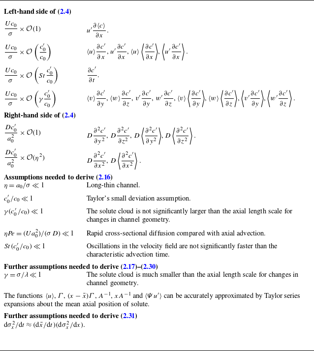
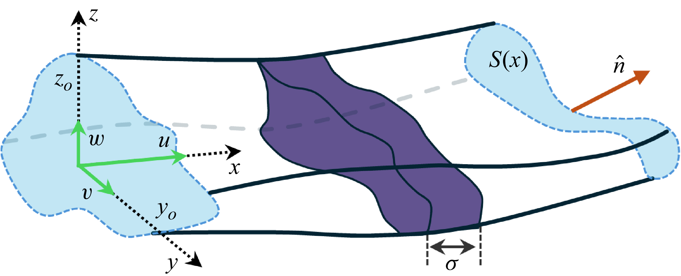
 σ
 S(x)
 x
 n^
 y0
 z0
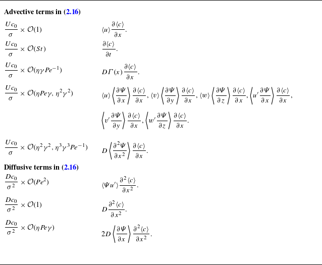

 a(x)=a0+0.2a0sin(x∗/400)
 (a)
 (a)
 (b−d)
 (b),(c)
 (d)

 (a)
 l0
 h(x)
 (b)
 Ψ
 y∗=y/h0
 z∗=z/h0
 Ψ
 u′

 (a)
 (b)
 (c)
 Pe=a0⟨u⟩/D
 γ=σ/λ
 ηPe

 y∗
 x∗
 (a)
 (a)
 z
 (b)
 (c)
 (a)

 (a)
 z0
 z0f(x)
 A(x)
 (b)
 f(x)
 (z0f)′
 ln(σx2/A)
 ln(σx2/A)
 ln(σx2/A)
 (i)
 (ii)
 (iii)

 (a)
 (b)
 σx2=0.3x∗+50sin(2πx∗/600)+300
 σx2=50sin(2πx∗/600)+300
 (i)
 (ii)
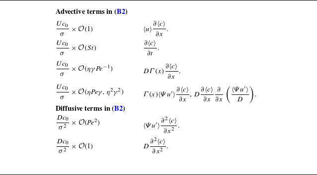


 Open access

