


Introduction
An objective of field studies on glaciers is to use measurements of velocity, surface slope, ice thickness and, perhaps, internal radio-reflecting layers to calculate stresses and deformation rates at depth. These can then be used to determine the location of the sites of higher resistance and to infer something about the mechanics acting at these sites. The deformation pattern can also be used to calculate the disruption to the stratigraphy of deep cores and the flow trajectories within the ice.
Many studies of ice flow start with a model for basal conditions and use this, together with the field equations, to calculate results that can be compared with measured data. Examples of this approach are in Reference JensenDahl-Jensen (1985) for Dye 3, Greenland, and Reference MacAyealMacAyeal (1987) for the Ross Ice Shelf. This approach has the advantage that the calculations follow the physics from cause to effect, but the difficulty is that trial-and-error techniques are required in formulating the, generally unknown, basal boundary conditions until agreement is obtained with measurements.
A more direct approach is to make the inverse calculation by using measured data to infer deep conditions. This has been done by Reference MacAyeal, Bindschadler, Shabtaie, Stephenson and BentleyMacAyeal and others (1987) to determine the force budget of the Crary Ice Rise complex, by Reference Bindschadler, Stephenson, MacAyeal and ShabtaieBindschadler and others (1987) at the mouth of Ice Stream B, by Reference Frolich, Mantripp, Vaughan and DoakeFrolich and others (1987) to describe the flow of Rutford Ice Stream over a basal disturbance, by Reference Whillans and JohnsenWhillans and Johnsen (1983) for the Byrd Station Strain Network, and by Reference Whillans and JezekWhillans and Jezek (1987) for the Dye 3 strain grid.
A similar approach is taken here in that stresses and velocities at depth are calculated from measured data. The preceding paper in this series (Reference Veen and WhillansVan der Veen and Whillans, 1989; hereafter referred to as part I) provides the theoretical framework and a description of the solution method. In short, surface velocities are used to calculate vertical shearing at the surface (by solving the force-balance equation) from which velocities at some depth below the surface are calculated. These velocities are used to compute vertical shearing at that depth, which yields velocities, at the next depth layer. Thus, by progressively going downward, velocities and stresses are calculated throughout a section of the glacier. The results of these calculations are basal drag and basal velocities.
This contribution discusses results of such a downward calculation for the Byrd Station Strain Network, West Antarctica. The major objective is to conduct a sensitivity study, and identify potential error sources affecting the results.
The Byrd Station Strain Network (BSSN)
The BSSN is a series of 52 almost square quadrilaterals with sides about 3 km long extending over 163 km from 6.3 km on the Amundsen Sea side of the ice divide (lat. 79°10’S., long. 112°57’ W.) to New Byrd Station (lat. 80 ° S., long. 119 30’W.). Because the network follows more or less the regional surface slope, it approximates the flow path for the ice (Fig. 1). In 1963–64 and 1964–65, and again in 1967–68, the network was surveyed for relative ice movement by the U.S. Geological Survey. Net surface mass balances have been obtained from changes in pole heights over periods of up to 8 years (Reference WhillansWhillans, 1978).
Elevation (contour interval = 5 m) and ice velocity along the Byrd Station Strain Network (BSSN) (from Reference Whillans and RobinWhillans, 1983). For clarity, velocities are plotted beside the network instead of in it. The data used here are from the part of the strain network shown as a solid line. NBS, New Byrd Station; OBS, Old Byrd Station

Because the BSSN consists of only two parallel rows of stakes, lateral stress gradients cannot be determined. This means that the force budget can only be calculated along the axis of the network, and lateral gradients in lateral drag and tension cannot be included. However, strain-rates involving the cross-flow horizontal direction are generally much smaller than those along the flow direction (Reference Whillans and JohnsenWhillans and Johnsen, 1983). Therefore, the restriction is probably not a major limitation to plane flow.
Surface velocities are nearly parallel to the network until about 141 km from the ice divide, or 25 km up-glacier of New Byrd Station. Only the part of the network with distinct along-network flow is considered. Thus, the part of the flow line considered here extends from 6 to 141 km down-slope of the ice divide (Fig. 1).
The measured data are gridded to a regular 3 km grid using cubic-spline interpolations. Such a regular grid is most convenient for the force-budget calculation. Because the grid spacing is close to the distance between the poles (about 3 km), the gridded data differ only slightly from those measured.
The surface and bed elevations (from Reference WhillansWhillans, 1979) are shown in Figure 2 (upper panel). The average surface slope along the BSSN is 0.002 but locally it varies from almost zero to 0.004. The bed is relatively rugged, with undulations of up to a few hundred meters over several kilometers but there does not seem to be a dominant wavelength for the basal variations.
Data from the right-hand row of stations in the BSSN, gridded to a regular 3 km interval

The horizontal surface velocity (Fig. 2, third curve) increases steadily along the flow line, but, as Figure 3 shows, there are important variations in velocity gradient. A concern might be whether there are velocity fluctuations at shorter scales than the station spacing of 3 km can resolve. However, a small strain grid at 112 km from the ice divide with a station spacing of 500 m (Reference Dewart and WhillansDewart and Whillans, 1970) has been used to determine that there are no short-scale slope or strain-rate variations.
Driving stress and stretching at the surface (έχχ = ∂u/∂х) along the BSSN flow line

The vertical velocity is taken to be equal to minus the surface net-accumulation rate (Fig. 2, lowest curve; from Reference WhillansWhillans, 1978). This net-accumulation rate shows large variability, temporal as well as spatial. The inter-annual variability can be as much as 40 kg m−2 a−1, but the long-term average shows a pattern similar to the short-term averages; thus the spatial variations may be considered stable in time. The high accumulation rates near the ice crest are most likely the effect of orographic forcing.
By assuming that the vertical velocity at the surface is equal to minus the surface-accumulation rate, steady-state conditions along the flow line are adopted. This is in agreement with the overall current mass balance which indicates that ice discharge exceeds input by only about 20% (Reference WhillansWhillans, 1977). (New results on the tilting of the Byrd Station core hole (personal communication from N. Gundestrup, 1988) indicate that the thinning rate is a little larger than the 20% calculated earlier.) A uniform thickening or thinning along the flow line (a constant error in the vertical velocity) does not influence the results.
Horizontal gradients in the vertical velocity could be important. However, horizontal variations in the rate of thickness change are small and within the error limits of the accumulation data (0.02 m a−1; Reference WhillansWhillans, 1978). Moreover, the close association of slope and strain-rate patterns indicates that the surface topography is related to deep ice-flow effects rather than transient effects. It is thus appropriate to suppose that the position of the surface is steady in time.
For the force-budget calculations, two important derived quantities are the driving stress (τd) and surface stretching (έ χχ ). Both are shown in Figure 3. The mean value of the driving stress is about 40 kPa (0.4 bar), but variations in it can be as large as this mean value. At 105 km down-glacier of the divide, the driving stress is almost zero, while at 141 km it reaches the value of 100 kPa. Similarly, variations in the surface stretching rate are of the same order of magnitude as the mean value. These variations in driving stress and stretching play central roles in the force-budget calculations.
For calculations at depth, the temperature profile must be prescribed. For this we use the profile measured in the Byrd Station bore hole (data from B.L. Hansen, given in Reference Robin and RobinRobin, 1983). The measured profile shows an unusual gradient near the surface, which is attributed to the drilling operation. Therefore, the upper 10% of the ice is taken to be isothermal, with a temperature equal to the annual mean temperature (−28 ° C; Fig. 4). Also, no detailed temperature measurements are available for the lowest 350 m of the bore hole, because of upwelling water encountered at the base of the ice. Therefore, the basal temperature (−1.6°C) calculated from the overburden pressure and the observed presence of basal water (Reference Robin and RobinRobin, 1983), is used and values interpolated over the interval.
Temperature profile measured in the Byrd Station bore hole (data from B.L. Hansen; reported by Reference Robin and RobinRobin (1983)). Scaled depth is represented by s. In the upper part, the data are questioned and it is assumed that this part of the glacier is isothermal, as shown by the broken line

The temperature profile measured at Byrd Station is scaled to ice thickness and applied along the entire strain network. Measured near-surface temperatures show no systematic change along the strain network. Presumably, the usual lapse rate over the 300 m elevation change does not apply because of proximity to the ice crest and because air masses can arrive from many different directions to affect surface temperatures. Radio-echo returns from the bed are locally bright even near the ice crest and so there is probably basal water all along the strain network. Thus, surface and basal temperatures vary little, and applying the Byrd Station temperature profile to the entire up-glacial flow line is a reasonable approximation. Also, as is shown below, the results are not critically sensitive to the temperature profile.
Results
Basal drag and velocity
The major limitation to confidence in the results is due to the constitutive relation for ice. The temperature-dependence of the rate factor in Glen’s law is relatively well established and follows the Arrhenius relation A = A0 exp(−Q/RT), where Q is the activation energy (60 kJ mol−1), R is the gas constant (8.314 J mol−1 K−1), and T is temperature. (A is equal to B−n in the nomenclature of Part I.) The value of A 0, however, is known within a factor of 5 at best (Reference HookeHooke, 1981; Reference Paterson and BuddPaterson and Budd, 1982). As can be seen from inspection of the equation for force balance (equation (31) or (39) in part I), if a large value is chosen for A 0 (soft ice), longitudinal stresses and stress gradients are unimportant near the surface and the deep shear stress is almost equal to the driving stress. Conversely, a small value (stiff ice) leads to very large and unrealistic stress variations at depth.
This is illustrated in Figure 5 for three calculations; very stiff ice (A 0 = 2.34 × 10⁴ kPa−3 a−1), intermediate ice (A 0 = 2.34 × 10⁵ kPa−3 a−1), and very soft ice (A 0 = 2.34 × 10⁶ kPa−3 a−1). Two orders of magnitude in softness are encompassed by these three examples, with the intermediate value corresponding to the value recommended by Reference Paterson and BuddPaterson and Budd (1982). In all three calculations, the temperature profile shown in Figure 4 is used.
Calculated ratio of basal drag and driving stress, and ratio of basal velocity to surface velocity along the BSSN. The three curves shown correspond to very soft ice (----). intermediate ice (—), and a very stiff ice. (−−−). In the lower panel, all negative values are plotted as zero. These negative velocities occur in the bottom 4% of the ice thickness in the soft-ice case and cannot be realistic.

The ratio of basal drag to driving stress for each of the three runs is shown in Figure 5 (upper panel). Fluctuations are smallest for the soft ice and largest for the stiff ice, as expected. An exception occurs at 105 km, where the soft-ice curve has a pronounced minimum, while the other two curves are near a maximum there. This is because, in the soft-ice case, there are very large horizontal velocity gradients at depth (lower panel) of opposite sense to those measured at the surface and the associated longitudinal stress gradients result in the unusual basal drag at that site. Figure 5 shows that basal drag for intermediate ice is within 30% of the value of the driving stress, and that varies by 100% along the flow line (Fig. 3).
In contrast to the basal drag, which shows a similar pattern in all three cases, basal velocities (Fig. 5, lower panel) are completely different for the three calculations. For stiff ice, the basal velocity is only slightly smaller than the surface velocity, so the bulk of the flow is calculated to be due to basal sliding. For soft ice, on the other hand, along most of the strain net virtually all motion is due to internal deformation with small, or even, unrealistically, negative basal velocities. In the intermediate case, basal sliding and internal deformation are, on average, roughly of equal importance, and play varying roles.
For all three model runs, the vertical resistive stress (Rzz ) is calculated explicitly. Compared to the weight of the ice above, or lithostatic stress, however, this stress is very small. At the base of the ice, deviations from lithostatic are less than 50 kPa or 0.1% of the lithostatic stress. Neglecting bridging effects by setting Rzz equal to zero everywhere alters basal drag by at most 4 kPa (Fig. 6).
Effect of bridging effects on basal drag. Shown is basal drag calculated by neglecting bridging effects, divided by basal drag from the complete calculation

The two places where bridging effects are most important (near the divide and at 105 km) correspond to the regions where the basal drag is very small. The basal drag at these sites is calculated to be small because the driving stress is small (Fig. 3) and the effect of longitudinal stress gradients has made basal drag even smaller (Fig. 5). However, in ordinary examples, it is appropriate to neglect bridging effects.
Zones of enhanced creep
According to the conventional flow law, the creep of ice is very non-linear, with the non-linearity described by the square of the effective shear stress. This effect may lead to local zones of stress softening and creep enhancement. Such stress softening has been considered in some sliding theories for small-scale features, but has not been addressed for large-scale flow. The square of the effective shear stress (T2 e) is a measure of the stress effects on the viscosity of the ice. Its value along the studied region of the Byrd Station Strain Network is depicted in Figure 7.
Effective shear stress squared, T2 e in units of kPa2 versus distance along flow line and depth, scaled to the ice thickness. This example is for n = 3 and the intermediate-valued rate factor.

The quantity, τ2 e, varies by a factor of about two near the surface and about three near the bed. Near-surface variations in the effective shear stress are associated with longitudinal strain-rates, or surface stretching (Fig. 3). The increased stretching, in turn, is correlated with ice flow up reversed bed slopes (Fig. 2). Lateral spreading and side shear are not included in this calculation, but these strain-rates are smaller than the longitudinal stretching (Reference Whillans and RobinWhillans and Johnsen, 1983) and so they do not affect the results of Figure 7 in an important way.
In general, the surface and basal values of differ from one another by a factor two to three. This is much less than the depth variation of the temperature-dependent rate factor (which varies by a factor of 20 from top to bottom). It thus seems that the role of τ2 e and stress softening is not centrally important to the flow of inland ice near Byrd Station. It may play a more critical role elsewhere if horizontal stresses are large as, for example, where ice flow funnels into an ice stream or outlet glacier.
Sensitivity of the Results
Input data
The ice thickness, or bed profile, derives from airborne radio echo-sounding that failed to obtain bed returns at many places. The calculated values of basal drag are, however, not very sensitive to the bed profile. In fact, replacing the bed shown in Figure 2 by a smooth (fourth-order) polynomial yields almost the same results as shown in Figure 5.
The surface slope is critical because it directly affects the calculation of basal drag through the driving stress. The driving stress includes both thickness and slope but potential proportional errors in slope are much larger. The slopes were measured by taking reciprocal vertical angles with a Wild T-3 theodolite and are believed accurate to better than 3 × 10⁻⁴ rad. That translates to an uncertainty of only 6 kPa in driving stress or basal drag, which is unimportant.
A constant systematic error in the surface velocity has little effect on the calculated results. For example, increasing the surface velocity by 0.5 m a−1 along the entire flow line yields exactly the same values for basal drag.
The force-balance calculation is more sensitive to velocity gradients. These are obtained from the repeat surveys of the strain grid and are accurate to about 10−5 a−1 (relative velocity between stations accurate to 0.02 m a−1). The importance of relative velocity is illustrated in Figure 8, in which the surface velocity at 69 km, where there is an important deviation of basal drag from driving stress (Fig. 5), has been increased from 4.9 to 5.1 m a−1, or ten times the measurement uncertainty. This change affects basal drag in a region extending about 10 km (3–4 ice thicknesses) in both directions. The calculated basal drag is mainly affected by the curvature of the surface-velocity profile, or strain-rate gradient. When the second derivative of the velocity decreases, basal drag also decreases. The experiment in Figure 8 is, however, for an extreme change in input data, and it is evident that the calculated basal variations are not very sensitive to realistic measurement uncertainties.
Effect of a deviation in the surface velocity (indicated by the dashed curve) on the drag at the base. The alteration in strain-rate is ten times the estimated measurement precision

The input data must be treated carefully. Usually, the input data are available at irregularly spaced points but the calculations are most straightforward if the values are on a regular grid. The spacing of the grid should be chosen such that its grid points are as close as feasible to the points where data are available. This assures that the difference between gridded and actual data is minimal, while retaining small-scale features. When a smaller calculation grid is used, results are heavily influenced by the interpolation scheme, to such an extent that very different variations in basal drag are obtained according to the interpolation scheme used. This proved not to be a major issue with the results presented here because the data spacing of 3 km is very nearly regular and the calculation points are very close to the survey points.
Temperature at depth
An important source of uncertainty lies with the constitutive relation for ice, and, more specifically, the rate factor, as is illustrated in Figure 5. The value of the rate factor plays a major role in determining to what extent basal drag deviates from the driving stress. For a large rate factor (soft ice), the longitudinal stretching term is unimportant and a close balance between basal drag and driving stress results. This proves to be a crucial issue with calculated deep velocities, but it is much less important for calculated basal drag.
The rate factor is a strong function of temperature, or equivalently, depth. This affects the budget of forces because the rate factor influences the calculated longitudinal tension. The results are not, however, very sensitive to the depth variation in rate factor. This is illustrated in Figure 9, which shows the ratio of drag at the base of an isothermal ice-sheet (−28 °C) to that calculated with the temperature profile shown in Figure 4. In both cases, the intermediate-valued rate factor, A 0 = 2.34 × 10⁶ kPa−3 a−1, is used. The difference between the two calculations is generally insignificant. The largest proportional deviation is at 105 km, where the driving stress and basal drag are very small. The maximum deviation is only 4 kPa.
Effect of temperature profile on calculated basal drag. Shown is the drag at the base of an isothermal glacier, divided by the basal drag calculated with the temperature profile shown in Figure 4

The weak sensitivity of the force budget to the temperature profile arises because the measured profile (Fig. 4) is nearly isothermal for the upper 70% of the thickness. Horizontal stresses in the bottom 30% do not play a major role in the overall budget of forces and changing deep temperature by 27 °C, as in Figure 9, has only moderate effects on the calculated basal drag.
The constitutive relation
The calculations described above are based on a non-linear constitutive relation with exponent n = 3. However, as Reference Doake and WolffDoake and Wolff (1985) argued, field data indicate that a linear flow law (n = 1) may also be appropriate to describe the deformation of polar ice. We therefore turn now to investigate the effect that the value of n has on the calculated results.
Figure 10 shows the outcome of two model runs, one in which the stiff-ice, non-linear flow law is used (n = 3, A 0 = 2.34 × 10⁻⁴ kPa−3 a−1), and one based on the linear relation (n = 1, A 0 = 5.85 × 10⁸ kPa−1 a−1). In both calculations, the temperature-dependence of the rate factor is prescribed through the Arrhenius relation, using the measured temperature profile shown in Figure 4.
The similarity between the two curves shown in Figure 10 is striking. Although the value of n affects the results in a quantitative manner, the general pattern remains unchanged. The reason for this is that the effective stress is relatively constant with depth (Fig. 7). This is a valuable result, and so the generalized flow law,
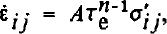
can be approximated as
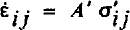
where A’ = ATn-1 e may be separated into parts, in which most of the depth variation is associated with the temperature-dependence of the rate factor A. The quantity, Tg−1, varies much less with depth (Fig. 7) but it accounts for all the variation with distance along the flow line. Thus, by choosing the value of A’ appropriately, the results for both n = 1 and n = 3 can be rather similar, with differences arising mainly because the effective stress varies along the flow line.
Comparison of basal drag calculated using a linear flow law (---) and using the non-linear one (—).

A major reason for developing this theory was to avoid the limitation in prior related works by Reference Whillans and RobinWhillans and Johnsen (1983) and Reference Whillans and JezekWhillans and Jezek (1987) that n = 1. The present results indicate, however, that the value of n is not critical and the linear, Fourier decomposition approach taken by those authors is appropriate. We do, however, favor the current method because of its flexibility and generality.
Discussion
An objective of force-budget calculations is to identify and locate the resistive forces that oppose the flow of ice masses. Most notably, interest is in the spatial distribution of basal drag and its deviations from the driving stress. There are, of course, limitations to such calculations posed mainly by uncertainties in the rate factor in the constitutive relation for polar ice. However, because the calculation here does not include any assumptions other than that of plane flow, it is an improvement over earlier theories. Moreover, the calculations need not be restricted to plane flow but, because the BSSN contains only two rows of stations, there are no data on transverse strain-rate gradients and a full three-dimensional calculation is not possible.
The results obtained for the BSSN show that basal drag deviates from the driving stress by typically only 5–10 kPa. Thus, for simple calculations, the basal drag can be set equal to the driving stress. Along the BSSN, the basal drag follows the driving stress and varies through the large range of 0–80 kPa over distances of about 15 km.
These results contrast with models commonly used to represent the flow of glaciers and especially of inland ice. In these, the areally meaned basal drag is taken as equal to the areally meaned, driving stress, which is appropriate. However, sliding relations are usually developed to link local stress and local sliding, and it is not clear how local sliding laws can be applied to the average flow. As Figures 3 and 5 show, basal drag and velocity both vary by large amounts. Frictional resistance is focused at certain sites, for example near 65 and 88 km, which are where the sliding rate is least. Conversely, regions of small drag, for example around 70 and 105 km, have large sliding. This linkage is the reverse of that used in many sliding laws.
These large basal drag variations are probably linked to the distribution of basal lubrication. The bed may be better lubricated where the basal drag is low and sliding rate high. The high-drag, slow-sliding “sticky spots” are not clearly correlated with basal relief (Fig. 2) and Reference Whillans and JohnsenWhillans and Johnsen (1983) provided evidence of well-lubricated sites, probably subglacial lakes, that are not tied to basal topography. The flow of the ice sheet is evidently controlled at separated “sticky” sites of large drag and slow slip. An understanding of the dynamics of the ice sheet requires an understanding of what controls these sites of high drag.
There is a limit to the detail in basal variation that can be calculated by the current technique. Because calculations start with measured surface effects as input, meaningful variations at the bed cannot be determined for wavelengths shorter than contained in the data. However, a detailed network at 112 km shows that there is no more detail than is resolved by the main grid (Reference Dewart and WhillansDewart and Whillans, 1970). This is in line with theoretical predictions (Reference HutterHutter, 1983, chapter 4; Reference Whillans and JohnsenWhillans and Johnsen, 1983) that short-wavelength features are damped out at depth and do not occur at the surface. Thus, basal variations at a detail finer than those obtained here cannot be obtained.
In inverse calculations, such as those here, in which measured effects are used to calculate their cause, the results can be very sensitive to small errors in the input data. The effect of errors in the driving stress on calculated stresses at depth is relatively straightforward to assess. Uncertainties in strain-rates (measurement errors for the BSSN are about 10−5a−1) have only a small effect on calculated deep stresses, as shown in Figure 8. Basal velocities may be affected more, but these are less reliable already given the uncertainty in the value of the rate factor. Tests were also made by changing the grid spacings (horizontal and vertical) in the calculations. In all, the resulting stresses at depth are not critically sensitive to measurement errors or to the numerical scheme.
Conclusions
The scheme for calculating stresses at depth from surface data is a very powerful technique and no assumptions need be made in the force-budget calculation. The method is used with measured surface effects to determine the basal stress and velocity variations that cause the surface effects. We know of no theoretical limitation to the technique.
The form of the flow law affects the results of the calculation. The pattern of calculated stress is not overly sensitive, but deep velocities do depend critically on especially the stiffness or rate factor. Any steady-state flow law could be used and we speculate that an anisotropic flow law would be more appropriate. At Byrd Station, the ice crystals are closely aligned at depths between 55 and 83% of the thickness (Reference Gow and WilliamsonGow and Williamson, 1976). Over that interval the ice should be stiff to horizontal stresses and soft to vertical shear. We are not aware of a fully developed flow law for such anisotropic ice but one should be developed and tested with the present data. In line with our experiments based on the conventional flow law, we expect use of an anisotropic relation would produce a pattern of deep-stress variation similar to that calculated here, but basal velocities would be different.
The confirmation that basal friction is restricted to certain separated sites has important implications to theoretical developments on the mechanics of sliding. Existing theory is for horizontally uniform conditions. Commonly, however, the basal drag is concentrated at sites about 10–20 km apart. Between these sites the drag is small and the sliding larger. What counts to the overall sliding of the glaciers is the size of and mechanics at the high-drag sites.
Acknowledgements
This work was supported by U.S. National Science Foundation grant DPP-8517590 and the Ohio State Post-Doctoral Fellowship Program. We thank K. Hutter and a referee for comments. This was typed by C. Gribbin and M. Hill. This is Byrd Polar Research Center contribution number 599.



