1 Introduction
In nature and many engineering applications, numerous examples can be found where one fluid interacts with another fluid and results in a destabilized interface. In addition, instabilities are responsible for several physical phenomena from micro-jet drop formation (Herrada et al. Reference Herrada, Montanero, Ferrera and Gañán-Calvo2010) to ocean wave currents (Bremond, Clanet & Villermaux Reference Bremond, Clanet and Villermaux2007). One of the most commonly encountered applications where an interface is destabilized is in liquid atomization (Lefebvre Reference Lefebvre1989; Lasheras & Hopfinger Reference Lasheras and Hopfinger2000). Liquid sheet destabilization results in a deformed interface, leading to an increase in the liquid–vapour interfacial area, which is one of the objectives of primary atomization. In most practical spray applications, a liquid jet ejected from a nozzle is shaped into a cylindrical annular sheet prior to being impacted by high-speed air at either interface. Typically, such a configuration can be encountered in air-blast atomizers (Lozano et al. Reference Lozano, Barreras, Hauke and Dopazo2001; Duke, Honnery & Soria Reference Duke, Honnery and Soria2012), effervescent atomizers (Sovani, Sojka & Lefebvre Reference Sovani, Sojka and Lefebvre2001; Lhuissier & Villermaux Reference Lhuissier and Villermaux2013) as well as in other coaxial atomizers (Rehab, Villermaux & Hopfinger Reference Rehab, Villermaux and Hopfinger1997; Lasheras, Villermaux & Hopfinger Reference Lasheras, Villermaux and Hopfinger1998; Lasheras & Hopfinger Reference Lasheras and Hopfinger2000), where relative velocity-induced shear is the primary cause of destabilization. Atomization processes could be governed by several instability mechanisms. As two examples, the influence of both Rayleigh–Taylor (RT) and Kelvin–Helmholtz (KH) mechanisms has been shown to be important (Lasheras & Hopfinger Reference Lasheras and Hopfinger2000). The RT mechanism occurs in the presence of an unfavourable density stratification at an interface in an acceleration field (Sharp Reference Sharp1984). The KH mechanism, on the other hand, occurs due to difference in velocities across an interface (Taylor Reference Taylor1950). While each of these mechanisms has been shown to be important in its own right, the case where they occur together is less studied.
We will specifically focus our attention on primary atomization and discuss the relevance of our work in that context. Most primary atomization processes currently rely on high shear between the liquid and gas streams (KH instability) to destabilize an interface. Any occurrence of RT instability is introduced as a secondary effect, as has been shown through a large body of experimental (Clanet & Villermaux Reference Clanet and Villermaux2002; Villermaux & Clanet Reference Villermaux and Clanet2002; Marmottant & Villermaux Reference Marmottant and Villermaux2004; Bremond et al. Reference Bremond, Clanet and Villermaux2007) and computational work (Jarrahbashi & Sirignano Reference Jarrahbashi and Sirignano2014; Jarrahbashi et al. Reference Jarrahbashi, Sirignano, Popov and Hussain2016). In contrast, the current study proposes a novel way of destabilizing the interface using primary RT instability. In such a case, the liquid sheet could be simultaneously destabilized by a relative velocity between the atomizing gas and the liquid phase, as well as by the radial motion of the liquid sheet when it exits the atomizer. During the course of this study, we will show the advantages of using radial acceleration to destabilize an interface. Further, we will also show that, for a given dimensionless energy, the characteristic destabilization length scale due to radial acceleration is significantly smaller than the length scale generated from conventional interface destabilization methodologies using axial relative velocity.
The literature related to the KH mechanism on annular liquid sheets is very extensive. Detailed reviews of KH instability as applicable to primary atomization can be found in Sirignano & Mehring (Reference Sirignano and Mehring2000), Dumouchel (Reference Dumouchel2008) and Eggers & Villermaux (Reference Eggers and Villermaux2008). Most studies of annular liquid sheets are limited to understanding the influence of two-dimensional (axisymmetric) disturbances. An instability analysis of annular sheets subjected to three-dimensional disturbances was first investigated by Panchagnula, Sojka & Santangelo (Reference Panchagnula, Sojka and Santangelo1996). Since experimental observations on most atomizers have shown three-dimensional structures, it would be interesting to study the instability characteristics of an annular liquid sheet subject to such disturbances.
Relatively few studies have focused on RT instability on curved interfaces where the interface is radially accelerated inwards or outwards (Mikaelian Reference Mikaelian2005; Delale, Tryggvason & Nas Reference Delale, Tryggvason and Nas2008). Sharp (Reference Sharp1984) and Kull (Reference Kull1991) have provided detailed reviews of the literature on RT instability on planar and spherical interfaces. The work of Plesset (Reference Plesset1954) on a spherical interface and Mikaelian (Reference Mikaelian2005) on a cylindrical interface deserve special mention. Plesset (Reference Plesset1954) developed the stability theory for a spherical interface with radial motion by invoking the frozen-flow approximation and concluded that the destabilization characteristics depended on the direction and magnitude of the radial acceleration. Mikaelian (Reference Mikaelian2005) analysed RT instability of two fluids in an unfavourable density stratification in a cylindrical configuration introducing only circumferential disturbances. As with KH instability, both axial and azimuthal disturbances are relevant in RT instability as well (Velikovich & Schmit Reference Velikovich and Schmit2015). In addition, the combined effect of both KH and RT destabilization mechanisms has received scant attention especially on curved interfaces. The present study attempts to fill this void in the literature.
We draw our motivation to study the simultaneous occurrence of RT and KH instabilities on annular liquid sheets from the following four key findings from the literature. (1) The study of Santangelo & Sojka (Reference Santangelo and Sojka1995) reported a high-speed focused image holographic imaging study of the near-nozzle structures in effervescent atomizer sprays, where they observed the breakup of an annular liquid sheet into azimuthally placed ligaments. (2) The experimental work of Duke et al. (Reference Duke, Honnery and Soria2012) showed that the radial movement of a liquid sheet has a significant effect on its breakup characteristics. (3) A recent paper by Vledouts et al. (Reference Vledouts, Quinard, Vandenberghe and Villermaux2016) reported results from a set of elegant experiments on exploding spherical shells, pointing to the role of RT instability. (4) A recent theoretical report by Vadivukkarasan & Panchagnula (Reference Vadivukkarasan and Panchagnula2016) showed that three-dimensional helical modes were possible when cylindrical interfaces were destabilized through a combination of KH and RT instabilities simultaneously. We will discuss these papers in detail.
Santangelo & Sojka (Reference Santangelo and Sojka1995) reported a high-speed three-dimensional imaging study of near-nozzle structures in an effervescent spray. Their study showed that, at reasonably high gas-to-liquid ratios, the liquid is formed into an annular sheet which does not remain parallel, but expands outwards radially. In addition, this radially expanding liquid sheet disintegrates into a discrete number of ligaments which are placed in an azimuthal arrangement. This structure cannot be explained purely by the action of shear at the inner interface between the gas and liquid streams, because the KH mechanism in these configurations yields only axisymmetric disturbances as the dominant instability mode. The role of the radial motion of the annular liquid sheet, especially acceleration, has been ignored in attempts to understand this work. Through this study, we would like to include the effect of acceleration to show that it could explain azimuthal structures in primary atomization processes.
Duke et al. (Reference Duke, Honnery and Soria2012) studied the breakup structures formed by the interaction of an inner gas stream with an annular liquid sheet using high-speed imaging. They show that nearly periodic azimuthal ligaments are possible under certain parametric conditions. However, the source of acceleration in creating these azimuthal instabilities is the finite-amplitude flapping motion of the annular liquid sheet induced by the primary KH instability. Therefore, the flapping motion induced by the KH instability provides the acceleration field for secondary RT instability to be triggered. This is similar to the report of Lasheras et al. (Reference Lasheras, Villermaux and Hopfinger1998) and summarized in Lasheras & Hopfinger (Reference Lasheras and Hopfinger2000). While they alluded to the importance of radial motion in their study, we would like to consider a situation where velocity shear and acceleration are simultaneously present.
Vledouts et al. (Reference Vledouts, Quinard, Vandenberghe and Villermaux2016) recently reported an experimental study of exploding spherical shells. Their experiments were very elegant and clearly outlined the effect of radial motion on the stability of a curved interface. They trapped a small quantity of
 $\text{H}_{2}+\text{O}_{2}$
mixture inside a spherical bubble and used a laser source to ignite the mixture. The ensuing combustion reaction created a pressure field inside the shell that caused the spherical interfaces to expand radially, resulting in hole formation. They show that RT instability induced by the accelerating interface accompanied by unfavourable density stratification is responsible for these structures. To the best of our knowledge, this is the first experiment where direct evidence of the effects of acceleration normal to a thin curved liquid sheet have been quantified. Their work used spherical shells which are discrete objects undergoing radial expansion. In this study, we are interested in understanding the stability of an analogous system involving continuous flow inside an annular liquid sheet and a source of radial expansion at its core. Such a system would have to include both KH and RT instabilities due to additional velocity shear at the interfaces.
Vadivukkarasan & Panchagnula (Reference Vadivukkarasan and Panchagnula2016) studied the stability of a single cylindrical interface subject to both RT and KH instability mechanisms. They used linear instability analysis with the possibility of observing three-dimensional instability modes (both azimuthal and axial) at inception. From their study, they concluded that radial acceleration is significantly more destabilizing than axial shear (KH instability) and that such radial motion could result in the formation of helical modes. However, their conclusions were drawn on a simpler problem where only a single cylindrical interface was modelled. In addition, they did not validate their assumption related to the frozen-flow approximation. While their work provided pointers towards the importance of radial motion even in the presence of shear, no conclusive information on its relevance to a real engineering system could be obtained.
This study aims to understand the effect of the simultaneous action of RT and KH mechanisms on an annular liquid sheet as applied to primary atomization processes. In order to conduct a systematic study, three cases are considered herein: (1) pure KH instability, where radial acceleration is set to zero; (2) pure RT instability, where relative velocity between the three phases is set to zero; and (3) combined RT–KH instability, where no effect is suppressed. Three-dimensional disturbances are considered and a complete temporal linear stability analysis is developed. Three-dimensional modes are characterized by an axial wavenumber (
 $k$
) and a circumferential wavenumber (
 $m$
). The most unstable wavenumber pair, viz. the wavenumber pair that gives rise to the maximum growth rate, is referred to as (
 $k^{\ast },m^{\ast }$
). In addition, the cutoff wavenumber pair (axial and circumferential) determining the neutral stability, (
 $k_{c},m_{c}$
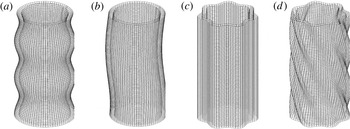
), has also been obtained. Given the three-dimensional nature of the destabilization, four different modes as shown in figure 1 are possible. They are (a) the Taylor mode (
 $k^{\ast }>0,~m^{\ast }=0$
), (b) the sinuous mode (
 $k^{\ast }=0,~m^{\ast }=1$
), (c) the flute mode (
 $k^{\ast }=0,~m^{\ast }>0$
) and (d) the helical mode (
 $k^{\ast }>0,~m^{\ast }>0$
). The Taylor mode corresponds to axisymmetric axial instabilities of a certain wavenumber with the circumferential wavenumber set to zero. The flute mode, on the other hand, corresponds to circumferential instabilities of a certain wavenumber with the axial wavenumber set to zero. Similarly, the helical mode is manifest when the interface is susceptible to disturbances with both axial and circumferential wavenumbers being non-zero. Helical modes in an annular liquid sheet system form the precursors to rupturing of the liquid sheet. Such rupturing action has been studied by Duke et al. (Reference Duke, Honnery and Soria2012) as well as by Park et al. (Reference Park, Huh, Li and Renksizbulut2004) and Zhao et al. (Reference Zhao, Liu, Tian, Xu, Li and Lin2014). The sinuous mode shown in figure 1(b) is a special case of a helical mode with
 $m^{\ast }=1$
. In both flute and helical modes,
 $m$
represents the number of imposed waves in the circumferential direction. As can be seen, it should be an integer to satisfy the periodicity condition in the circumferential direction.
Graphical representation of the different destabilization modes due to the combined RT–KH mechanism on an annular interface: (a) the Taylor mode (
 $k^{\ast }>0$
,
 $m^{\ast }=0$
); (b) the sinuous mode (
 $k^{\ast }=0$
,
 $m^{\ast }=1$
); (c) the flute mode (
 $k^{\ast }=0$
,
 $m^{\ast }>0$
); and (d) the helical mode (
 $k^{\ast }>0$
,
 $m^{\ast }>0$
). Here
 $k^{\ast }$
and
 $m^{\ast }$
are the most unstable axial and circumferential wavenumbers, respectively.

The paper is organized as follows. In § 2, a linear stability analysis of an annular liquid sheet system comprising incompressible, inviscid and immiscible fluids with combined RT and KH mechanisms is developed. In § 3, all the special cases of the general dispersion relation obtained are shown as a validation exercise. In § 4, the results of the current study are presented in detail. Section 4.1 presents a brief study of the results pertaining to KH and RT instability mechanisms occurring alone. Furthermore, § 4.2 elucidates the effect due to the combined action of RT and KH instabilities. In § 4.3, dimensionless energy partitioning for optimal destabilization is discussed. Section 5 presents a summary of the research along with key conclusions.
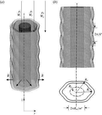
Schematic of an annular interface with the three (axial and circumferential) disturbances. Here,
 $(r,\unicode[STIX]{x1D703},z)$
indicate the cylindrical polar coordinates. (a) The annular interface of radii,
 $R_{i}$
and
 $R_{o}$
. An inner pipe of radius
 $R_{p}$
is indicated by the solid (black) cylinder. (b) Elevation view (top) depicting the axial wavelength; and schematic (bottom) showing the azimuthal wavenumber,
 $m^{\ast }$
, and the other geometric features. The dash-dotted inner circle indicates the radius,
 $R_{p}$
. Typically,
 $R_{p}\ll R_{i}$
, but is shown disproportionate for clear visualization. Also, the amplitude of the perturbation is small in comparison to the radii.

2 Mathematical formulation
We consider an infinite, inviscid annular liquid sheet of density
 $\unicode[STIX]{x1D70C}_{l}$
with the inner radius of the annulus being
 $R_{i}$
and the outer radius being
 $R_{o}$
(
 ${>}R_{i}$
) as shown in figure 2. Let (
 $r,\unicode[STIX]{x1D703},z$
) represent the coordinates in the radial, circumferential and axial directions, respectively, in the usual cylindrical polar coordinate description, with
 $(\hat{\boldsymbol{e}}_{r},\hat{\boldsymbol{e}}_{\unicode[STIX]{x1D703}},\hat{\boldsymbol{e}}_{z})$
representing the unit vectors in each direction. Let
 $t$
represent time. The annular liquid sheet encloses an inner gas of density
 $\unicode[STIX]{x1D70C}_{i}$
in the region
 $R_{p}(t)<r<R_{i}(t)$
, and an outer gas of density
 $\unicode[STIX]{x1D70C}_{o}$
in the region
 $r>R_{o}(t)$
. Here
 $R_{p}(t)$
is the radius of a ‘pipe’, which is a model for initiating motion in the radial direction (Mikaelian Reference Mikaelian2005; Delale et al.
Reference Delale, Tryggvason and Nas2008). As we will show later, the results are insensitive to the specific value of
 $R_{p}$
chosen as long as it is small in comparison with
 $R_{i}$
. The three fluids, viz. inner, liquid and outer fluids, are assumed to be moving with constant axial velocities given by
 $W_{i}$
,
 $W_{l}$
and
 $W_{o}$
, respectively. Here
 $i$
and
 $o$
represent the inner and outer gases, whereas
 $l$
represents the liquid sheet. The instantaneous position of the inner interface separating the inner gas and liquid is given by
 $r=r_{si}(\unicode[STIX]{x1D703},z,t)$
. Similarly, the instantaneous position of the outer interface separating the liquid and outer gas is given by
 $r=r_{so}(\unicode[STIX]{x1D703},z,t)$
. It is to be noted that the interface positions are functions of time,
 $t$
. Thermal effects are ignored and the fluids are assumed to be non-evaporating. In addition, interfacial tensions between the liquid sheet and the surrounding gas at the inner and outer interfaces are assumed to be constant and equal to
 $\unicode[STIX]{x1D70E}_{i}$
and
 $\unicode[STIX]{x1D70E}_{o}$
, respectively. Since the fluids are inviscid (and also since the flow field is irrotational), we can define a velocity potential
 $\unicode[STIX]{x1D719}_{j}$
in each fluid. Consequently, the velocity field
 $(u_{j},w_{j})$
in each fluid
 $j$
in the
 $(r,z)$
directions is given by
 $$\begin{eqnarray}u_{j}=\frac{\unicode[STIX]{x2202}\unicode[STIX]{x1D719}_{j}}{\unicode[STIX]{x2202}r},\quad w_{j}=\frac{\unicode[STIX]{x2202}\unicode[STIX]{x1D719}_{j}}{\unicode[STIX]{x2202}z}.\end{eqnarray}$$
Here,
 $j$
corresponds to the three subscripts,
 $l$
for the liquid sheet,
 $i$
for the inner fluid and
 $o$
for the outer fluid. In addition,
 $\unicode[STIX]{x1D719}_{j}$
in each fluid is governed by
 $$\begin{eqnarray}\unicode[STIX]{x1D6FB}^{2}\unicode[STIX]{x1D719}_{j}=0,\quad j=i,o,l.\end{eqnarray}$$
The interface boundary conditions that the velocity and pressure fields must satisfy can be classified into two sets: (1) kinematic boundary conditions and (2) dynamic boundary conditions. Kinematic boundary conditions require that a particle on the interface remains on it at all times, i.e. the material derivative of the particle position is zero. These conditions can be written as follows:
 $$\begin{eqnarray}\displaystyle & \displaystyle \left.\frac{\unicode[STIX]{x2202}\unicode[STIX]{x1D719}_{i}}{\unicode[STIX]{x2202}r}\right|_{r_{si}}=\frac{\unicode[STIX]{x2202}r_{si}}{\unicode[STIX]{x2202}t}+W_{i}\frac{\unicode[STIX]{x2202}r_{si}}{\unicode[STIX]{x2202}z}, & \displaystyle\end{eqnarray}$$
 $$\begin{eqnarray}\displaystyle & \displaystyle \left.\frac{\unicode[STIX]{x2202}\unicode[STIX]{x1D719}_{l}}{\unicode[STIX]{x2202}r}\right|_{r_{si}}=\frac{\unicode[STIX]{x2202}r_{si}}{\unicode[STIX]{x2202}t}+W_{l}\frac{\unicode[STIX]{x2202}r_{si}}{\unicode[STIX]{x2202}z}, & \displaystyle\end{eqnarray}$$
 $$\begin{eqnarray}\displaystyle & \displaystyle \left.\frac{\unicode[STIX]{x2202}\unicode[STIX]{x1D719}_{o}}{\unicode[STIX]{x2202}r}\right|_{r_{so}}=\frac{\unicode[STIX]{x2202}r_{so}}{\unicode[STIX]{x2202}t}+W_{o}\frac{\unicode[STIX]{x2202}r_{so}}{\unicode[STIX]{x2202}z}, & \displaystyle\end{eqnarray}$$
 $$\begin{eqnarray}\displaystyle & \displaystyle \left.\frac{\unicode[STIX]{x2202}\unicode[STIX]{x1D719}_{l}}{\unicode[STIX]{x2202}r}\right|_{r_{so}}=\frac{\unicode[STIX]{x2202}r_{so}}{\unicode[STIX]{x2202}t}+W_{l}\frac{\unicode[STIX]{x2202}r_{so}}{\unicode[STIX]{x2202}z}. & \displaystyle\end{eqnarray}$$
 $r=r_{si}(\unicode[STIX]{x1D703},z,t)$
and
 $r=r_{so}(\unicode[STIX]{x1D703},z,t)$
. The dynamic boundary conditions at the interfaces represent the discontinuity of pressure across each of the two interfaces, which arises due to surface tension and interface curvature. This condition can be written for the inner interface as
 $$\begin{eqnarray}p_{i}-p_{l}=\unicode[STIX]{x1D70E}_{i}\unicode[STIX]{x1D705}_{i}\end{eqnarray}$$
and for the outer interface as
 $$\begin{eqnarray}p_{l}-p_{o}=\unicode[STIX]{x1D70E}_{o}\unicode[STIX]{x1D705}_{o}.\end{eqnarray}$$
Here,
 $p_{j}$
(where
 $j=i,o,l$
) is the static pressure in each fluid at the interface; and
 $\unicode[STIX]{x1D705}_{i}$
and
 $\unicode[STIX]{x1D705}_{o}$
are the local curvatures of the inner and outer interfaces, respectively. Finally, it is required that the velocity field in each fluid is continuous and differentiable, which gives rise to the requirement that
 $$\begin{eqnarray}\left.\frac{\unicode[STIX]{x2202}\unicode[STIX]{x1D719}_{i}}{\unicode[STIX]{x2202}r}\right|_{r=R_{p}(t)}=\dot{R_{p}}(t),\quad \left.\frac{\unicode[STIX]{x2202}\unicode[STIX]{x1D719}_{o}}{\unicode[STIX]{x2202}r}\right|_{r\rightarrow \infty }=0.\end{eqnarray}$$
The unsteady Bernoulli equation relates the hydrodynamic pressure in each fluid to the velocity potential. This is given by
 $$\begin{eqnarray}p_{j}(r,t)=P_{j}(t)-\unicode[STIX]{x1D70C}_{j}\left[\frac{\unicode[STIX]{x2202}\unicode[STIX]{x1D719}_{j}}{\unicode[STIX]{x2202}t}+\frac{1}{2}|\unicode[STIX]{x1D6FB}\unicode[STIX]{x1D719}_{j}|^{2}\right].\end{eqnarray}$$
Here,
 $P_{j}(t)$
(
 $j=i,o,l$
) represents the stagnation pressure in each fluid. Equation (2.2) in each fluid, subject to the boundary conditions (2.3)–(2.6), describes the dynamics of the annular fluid system. We will now describe the mean flow field in the three fluids, viz. the inner gas, sheet fluid and the outer gas.
2.1 Mean flow description
The unperturbed mean flow is described by a condition where the interface position is assumed to remain cylindrical and axisymmetric at all times. The velocity vector field
 $\overline{U}_{j}$
in this flow is assumed to be
 $$\begin{eqnarray}\overline{U}_{j}=\frac{R_{j}{\dot{R}}_{j}}{r}\hat{\boldsymbol{e}}_{r}+W_{j}\hat{\boldsymbol{e}}_{z},\end{eqnarray}$$
where
 $j=i,o,l$
representing the three fluids; and
 $r_{sj}(\unicode[STIX]{x1D703},z,t)=R_{j}(t)$
with
 $j=i,o$
.
The velocity potential for this velocity field is given by
 $$\begin{eqnarray}\unicode[STIX]{x1D6F7}_{j}(r,z)=W_{j}z+R_{j}\dot{R_{j}}\ln \left(\frac{r}{R_{\infty }}\right),\quad j=i,o,l.\end{eqnarray}$$
Here,
 $R_{\infty }$
is introduced as a point that is sufficiently far away from the interface where the pressure remains constant and unaffected by the dynamics of the annular liquid sheet and where the fluid static pressure is
 $P_{o}$
(Burton, Waldrep & Taborek Reference Burton, Waldrep and Taborek2005; Ilinskii et al.
Reference Ilinskii, Zabolotskaya, Hay and Hamilton2012). We take
 $R_{\infty }=200R_{i}$
for all the simulations considered here. Recall that the inner fluid
 $i$
is present between
 $R_{p}(t)<r<R_{i}(t)$
. The inner interface at
 $R_{i}(t)$
is initiated into motion by the radial motion
 $\dot{R_{p}}$
at
 $R_{p}(t)$
, similar to Mikaelian (Reference Mikaelian2005) and Delale et al. (Reference Delale, Tryggvason and Nas2008). Since the fluids are incompressible and axial velocities are constant at all times, the cross-sectional area for each fluid is assumed to be constant at all times. In other words,
 $\unicode[STIX]{x03C0}(R_{i}^{2}-R_{p}^{2})=\unicode[STIX]{x1D6FF}$
and
 $\unicode[STIX]{x03C0}(R_{o}^{2}-R_{i}^{2})=\unicode[STIX]{x1D702}$
, with
 $\unicode[STIX]{x1D6FF}$
and
 $\unicode[STIX]{x1D702}$
being constants. A radially expanding circular pipe
 $R_{p}(t)$
is a model introduced to impart radial motion to the cylindrical interface as well as to mitigate the problem of logarithmic divergence of the velocity and pressure fields as
 $r\rightarrow 0$
. The radial velocity and acceleration can be obtained by differentiating the equation once and twice with respect to time. These equations are given by
 $$\begin{eqnarray}\displaystyle & \displaystyle R_{o}\dot{R_{o}}=R_{i}\dot{R_{i}}=R_{p}\dot{R_{p}}, & \displaystyle\end{eqnarray}$$
 $$\begin{eqnarray}\displaystyle & \displaystyle {\dot{R}}_{o}^{2}+R_{o}\ddot{R}_{o}={\dot{R}}_{i}^{2}+R_{i}\ddot{R}_{i}={\dot{R}}_{p}^{2}+R_{p}\ddot{R}_{p}. & \displaystyle\end{eqnarray}$$
 $\unicode[STIX]{x1D702}$
and
 $\unicode[STIX]{x1D6FF}$
are constants. The velocity field generated by
 $\unicode[STIX]{x1D6F7}_{j}$
in (2.9) satisfies the boundary conditions given by (2.3)–(2.6). In order for (2.4) and (2.5) to be satisfied, the mean pressures in the two fluids
 $P_{j}$
need to be related to the dynamical evolution of the interface radii. From this requirement, one can derive two equations governing the evolution of the interface radii
 $R_{i}(t)$
and
 $R_{o}(t)$
. They are given by
 $$\begin{eqnarray}\displaystyle R_{i}\ddot{R_{i}}\ln \frac{R_{i}}{R_{o}}+\left(\frac{1}{2}+\ln \frac{R_{i}}{R_{o}}\right)\dot{R_{i}}^{2}=\frac{1}{\unicode[STIX]{x1D70C}_{i}-\unicode[STIX]{x1D70C}_{l}}\left[\left(P_{i}-\frac{1}{2}\unicode[STIX]{x1D70C}_{i}W_{i}^{2}\right)-\left(P_{l}-\frac{1}{2}\unicode[STIX]{x1D70C}_{l}W_{l}^{2}\right)-\frac{\unicode[STIX]{x1D70E}_{i}}{R_{i}}\right] & & \displaystyle \nonumber\\ \displaystyle & & \displaystyle\end{eqnarray}$$
and
 $$\begin{eqnarray}\displaystyle R_{o}\ddot{R_{o}}\ln \frac{R_{o}}{R_{\infty }}+\left(\frac{1}{2}+\ln \frac{R_{o}}{R_{\infty }}\right)\dot{R_{o}}^{2}=\frac{1}{\unicode[STIX]{x1D70C}_{l}-\unicode[STIX]{x1D70C}_{o}}\left[\left(P_{l}-\frac{1}{2}\unicode[STIX]{x1D70C}_{l}W_{l}^{2}\right)-\left(P_{o}-\frac{1}{2}\unicode[STIX]{x1D70C}_{o}W_{o}^{2}\right)-\frac{\unicode[STIX]{x1D70E}_{o}}{R_{o}}\right].\hspace{-10.00002pt} & & \displaystyle \nonumber\\ \displaystyle & & \displaystyle\end{eqnarray}$$
2.2 Linear stability analysis
We will now study the stability of the mean flow field developed in the previous section subject to three-dimensional disturbances being imposed on the system. Let
 $a_{j}(t)$
(
 $j=i,o$
) be the infinitesimally small time-varying amplitudes of the imposed disturbances on the inner and outer interfaces. In other words,
 $a_{j}\ll R_{j}$
,
 $j=i,o$
. It can be shown that this system admits normal modes in the axial (
 $z$
) and circumferential (
 $\unicode[STIX]{x1D703}$
) directions for infinitesimal perturbations because of the infinite span in the
 $z$
direction and periodicity in the
 $\unicode[STIX]{x1D703}$
direction. Under this condition, the interface shape can be written as
 $$\begin{eqnarray}r_{sj}(\unicode[STIX]{x1D703},z,t)=R_{j}(t)+a_{j}(t)\text{e}^{\text{i}(\overline{k}z+m\unicode[STIX]{x1D703})}.\end{eqnarray}$$
The wavenumber pair (
 $\overline{k},m$
) is associated with the disturbances imposed in the axial (
 $z$
) and circumferential (
 $\unicode[STIX]{x1D703}$
) directions, respectively. Since the temporal stability of the system is being investigated, the axial wavenumber
 $\overline{k}$
is assumed to be real. In addition,
 $m$
is required to be an integer from the periodicity requirement in the circumferential direction. The corresponding velocity potential associated with the perturbation velocity field in each fluid is
 $\unicode[STIX]{x1D719}_{j}^{\prime }(r,\unicode[STIX]{x1D703},z,t)$
. The total velocity potential is therefore given by
 $$\begin{eqnarray}\unicode[STIX]{x1D719}_{j}=\unicode[STIX]{x1D6F7}_{j}(r,z)+\unicode[STIX]{x1D719}_{j}^{\prime }(r,\unicode[STIX]{x1D703},z,t).\end{eqnarray}$$
Here,
 $\unicode[STIX]{x1D6F7}_{j}$
is given by (2.9). Since (2.14) must satisfy (2.2), it can be shown with the help of (2.9) that
 $\unicode[STIX]{x1D719}_{j}^{\prime }$
must satisfy
 $$\begin{eqnarray}\unicode[STIX]{x1D6FB}^{2}\unicode[STIX]{x1D719}_{j}^{\prime }=0.\end{eqnarray}$$
The perturbation velocity fields given by (2.15) are also irrotational, similar to their respective mean velocity fields. From the normal mode ansatz invoked in (2.13) and (2.14), the solution to (2.15) must also be of the form
 $$\begin{eqnarray}\unicode[STIX]{x1D719}_{j}^{\prime }(r,\unicode[STIX]{x1D703},z,t)=g_{j}(r,t)\text{e}^{\text{i}(\overline{k}z+m\unicode[STIX]{x1D703})},\quad j=i,o,l.\end{eqnarray}$$
Substituting (2.16) into (2.15), one obtains the equation describing
 $g_{j}(r,t)$
as follows:
 $$\begin{eqnarray}\left[\frac{1}{r}\frac{\text{d}}{\text{d}r}\left(r\frac{\text{d}}{\text{d}r}\right)-\left(\frac{m^{2}}{r^{2}}+\overline{k}^{2}\right)\right]g_{j}(r,t)=0,\quad j=i,o,l.\end{eqnarray}$$
The solution to (2.17) for
 $g_{j}(r,t)$
is of the form
 $g_{j}(r,t)={\mathcal{A}}_{j}(t)\text{I}_{m}(\overline{k}r)+{\mathcal{B}}_{j}(t)\text{K}_{m}(\overline{k}r)$
. Here,
 $\text{I}_{m}(\overline{k}r)$
and
 $\text{K}_{m}(\overline{k}r)$
are modified Bessel functions of the first and second kinds of order
 $m$
, respectively. We invoke the conditions at
 $r=R_{p}(t)$
for
 $j=i$
and at
 $r\rightarrow \infty$
for
 $j=o$
(2.6). We then substitute the solution for
 $g_{j}(r,t)$
into (2.16) and use (2.14) and (2.9). Following this, the solution to the perturbation velocity potential can be obtained. The kinematic boundary conditions (2.3) are used to determine the coefficients
 ${\mathcal{A}}_{i}(t)$
,
 ${\mathcal{B}}_{i}(t)$
,
 ${\mathcal{B}}_{o}(t)$
,
 ${\mathcal{A}}_{l}(t)$
and
 ${\mathcal{B}}_{l}(t)$
, which are functions of time. By recalling that
 $a_{j}(t)\ll R_{j}(t)$
, only terms to
 $O(a_{j})$
(
 $j=i,o$
) are retained in the process of obtaining the linearized approximations of the above terms. Substituting the solutions obtained from implementing the boundary conditions, one finally obtains a set of two linear second-order ordinary differential equations for the time evolution of amplitudes
 $a_{j}(t)$
(
 $j=i,o$
corresponding to the inner and outer interfaces). They are given by
 $$\begin{eqnarray}\ddot{a}_{j}+f_{1}^{j}(\boldsymbol{Z}(\boldsymbol{t});\overline{k},m){\dot{a}}_{j}+f_{2}^{j}(\boldsymbol{Z}(\boldsymbol{t});\overline{k},m)a_{j}=0,\quad j=i,o.\end{eqnarray}$$
Here,
 $\boldsymbol{Z}(\boldsymbol{t})=[R_{i},{\dot{R}}_{i},\ddot{R}_{i},R_{o},{\dot{R}}_{o},\ddot{R}_{o}]^{\text{T}}$
is a vector comprising time-varying functions.
2.3 Prediction of instability characteristics using direct numerical time integration
It is to be noted that (2.18) are second-order ordinary differential equations involving time-varying coefficients because
 $f_{1}^{j}$
and
 $f_{2}^{j}$
are functions of time. The linearized growth of the perturbation amplitude can be obtained by integrating these equations with respect to time along with appropriate initial conditions similar to the initial value problem solved by Chen & Kirchner (Reference Chen and Kirchner1978). For each amplitude
 $a_{j}(t)$
, two initial conditions need to be specified in terms of
 $a_{j}(0)$
and
 ${\dot{a}}_{j}(0)$
. For a given set of flow parameters (
 $P_{j}$
,
 $P_{l}$
,
 $W_{j}$
,
 $W_{l}$
), fluid properties (
 $\unicode[STIX]{x1D70C}_{j}$
,
 $\unicode[STIX]{x1D70C}_{l}$
,
 $\unicode[STIX]{x1D70E}_{j}$
) and specified initial conditions
 $R_{j}(0)$
and
 ${\dot{R}}_{j}(0)$
,
 $R_{j}$
evolves in time as governed by the mean flow equations (2.11) and (2.12). The
 $R_{j}$
,
 ${\dot{R}}_{j}$
and
 $\ddot{R}_{j}$
values are obtained as solutions of these equations, which then are substituted in the functions
 $f_{1}^{j}$
and
 $f_{2}^{j}$
. Thus, the growth of the perturbation amplitude
 $a_{j}(t)$
is influenced by the time-varying mean flow condition. In general, it is not possible to find a closed-form solution to (2.18); hence, direct numerical time integration is the only recourse.
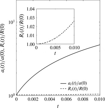
Plot of normalized disturbance amplitude growth (
 $a_{i}(t)/a_{i}(0)$
) and normalized inner radius (
 $R_{i}(t)/R_{i}(0)$
) versus time from direct numerical time integration. It can be seen that
 $a_{i}(t)/a_{i}(0)$
shows an exponential growth for short times whereas
 $R_{i}(t)/R_{i}(0)$
shows only polynomial growth in time (see inset). These results were obtained for
 $P_{i}=100~\text{N}~\text{m}^{-1}$
and
 $P_{o}=P_{l}=0$
. The other parameters chosen are
 $\unicode[STIX]{x1D70C}_{i}=1$
,
 $\unicode[STIX]{x1D70C}_{l}=\unicode[STIX]{x1D70C}_{o}$
,
 $\unicode[STIX]{x1D70E}_{i}=0.2$
and
 $\unicode[STIX]{x1D70E}=0$
. Also,
 $R_{i}(0)=0.005$
,
 ${\dot{R}}_{i}(0)={\dot{R}}_{o}(0)=0$
and
 $a_{i}(0)=10^{-6}$
,
 ${\dot{a}}_{i}(0)=0$
.

Figure 3 depicts the results obtained from such numerical time integration for the evolution of amplitude (
 $a_{i}(t)/a_{i}(0)$
) as well as the interface inner radius (
 $R_{i}(t)/R_{i}(0)$
) with time. As can be seen from figure 3,
 $a_{i}(t)/a_{i}(0)$
shows an exponential growth for short times, whereas
 $R_{i}(t)/R_{i}(0)$
shows only a polynomial growth in time (see inset). The latter observation is similar to the recent experimental observations of Vledouts et al. (Reference Vledouts, Quinard, Vandenberghe and Villermaux2016). In other words,
 $R_{i}$
(and similarly
 ${\dot{R}}_{i}$
and
 $\ddot{R}_{i}$
) is a slowly varying function of time. Consequently,
 $f_{1}^{j}$
and
 $f_{2}^{j}$
are also slow functions of time. We will now use this result to simplify (2.18), leading us towards an analytical dispersion relation.
2.4 Prediction of instability characteristics using frozen-flow approximation
As mentioned before, the functions
 $f_{1}^{j}$
and
 $f_{2}^{j}$
are slowly varying functions of time. One could therefore make an approximation that the coefficients in (2.18) are constants, following the work of Plesset (Reference Plesset1954) and Chen, Schrock & Peterson (Reference Chen, Schrock and Peterson1997). This approximation is based on the physical proposition that the movement of the interfaces and the rate of growth of disturbances on interfaces happen on disparate time scales. Though the interface radius (
 $R_{j}$
) is a function of time, which leads to interface velocity (
 $\dot{R_{j}}$
) and interface acceleration (
 $\ddot{R_{j}}$
), the time scale associated with this motion of the interface in the radial direction is much larger than that associated with the disturbance growth (
 $\dot{a_{j}}$
). Mathematically, this can be stated as
 $$\begin{eqnarray}\frac{\dot{a_{j}}(t)}{a_{j}}\gg \frac{\dot{R_{j}}(t)}{R_{j}},\quad j=i,o.\end{eqnarray}$$
Owing to this approximation, the coefficients in (2.18) can be assumed to be constants and one can obtain a closed-form solution for
 $a_{j}(t)$
in (2.18) of the form
 $a_{j}(0)\text{e}^{\overline{\unicode[STIX]{x1D714}}t}$
. This will further allow us to develop a closed-form dispersion relation for
 $\overline{\unicode[STIX]{x1D714}}$
as a function of the flow parameters. Following the above approach, (2.18) are reduced to two quadratic equations in
 $\overline{\unicode[STIX]{x1D714}}$
for the inner and outer interfaces. This yields a closed-form dispersion relation which can most conveniently be written in the form
 $|\unicode[STIX]{x1D63C}|=0$
where
 $[\unicode[STIX]{x1D63C}]$
is a
 $7\times 7$
matrix and is given in appendix A.
It may be recalled that
 $a_{i}$
and
 $a_{o}$
are the perturbation amplitudes at the inner and outer surfaces, respectively. The ratio of these two quantities, given by
 $\cos \unicode[STIX]{x1D713}=a_{i}/a_{o}$
, determines the phase angle,
 $\unicode[STIX]{x1D713}$
, associated with the dominant instability mode. For the case of a planar liquid sheet (Squire Reference Squire1953; Hagerty & Shea Reference Hagerty and Shea1955), only two values are possible for
 $\unicode[STIX]{x1D713}$
, viz.
 $0$
and
 $\unicode[STIX]{x03C0}$
. When
 $\unicode[STIX]{x1D713}=0$
, the two interfaces grow in phase; this mode is referred to as the sinuous mode. When
 $\unicode[STIX]{x1D713}=\unicode[STIX]{x03C0}$
, the instability mode is referred to as being varicose. However, for the case of an annular liquid sheet,
 $\unicode[STIX]{x1D713}$
is always between
 $0$
and
 $\unicode[STIX]{x03C0}$
, and also close to either of these two limiting values for an annular sheet in the thin limit. Following the work of Shen & Li (Reference Shen and Li1996), an equation has been obtained for
 $\unicode[STIX]{x1D713}$
as a function of the dimensionless parameters. Firstly, we have seen that this equation reduces to the relation of Shen & Li (Reference Shen and Li1996) when
 $m=0$
. From this equation,
 $\unicode[STIX]{x1D713}$
is close to
 $0$
for
 $\unicode[STIX]{x1D706}>0.9$
and for all values of
 $We$
considered in this work (
 $Bo$
plays no role). We can therefore conclude that the sheet is most susceptible to para-sinuous instability for all the parameter cases that we have studied in this work, similar to the findings of Shen & Li (Reference Shen and Li1996).
2.5 Dimensionless form of the dispersion relation
It is useful to study the stability of this flow in a dimensionless framework. The dimensionless numbers relevant to this study are: (1) Bond number
 $(Bo)$
, representing the ratio of radial acceleration force to the surface tension force; (2) Weber numbers (
 $We_{i}$
and
 $We_{o}$
), representing the ratios of the aerodynamic force due to the relative velocity to the surface tension force at each interface; (3) density ratios between the two pairs of fluids
 $(Q_{j})$
where
 $j=i,o$
; (4) the ratio of radial inertial force to surface tension
 $(S)$
; and (5) the ratio of inner radius to outer radius (
 $\unicode[STIX]{x1D706}$
). These dimensionless numbers can be written mathematically as
 $$\begin{eqnarray}Bo=\frac{(\unicode[STIX]{x1D70C}_{i}-\unicode[STIX]{x1D70C}_{l})\ddot{R}_{i}R_{m}^{2}}{\unicode[STIX]{x1D70E}},\quad We_{j}=\frac{\unicode[STIX]{x1D70C}_{l}(W_{j}-W_{l})^{2}R_{m}}{\unicode[STIX]{x1D70E}},\quad Q_{j}=\frac{\unicode[STIX]{x1D70C}_{j}}{\unicode[STIX]{x1D70C}_{l}},\quad S=\frac{\unicode[STIX]{x1D70C}_{l}{\dot{R}}_{i}^{2}R_{m}}{\unicode[STIX]{x1D70E}}.\end{eqnarray}$$
Here, two Weber numbers and two density ratios are required to characterize the system involving the two interfaces of the annular sheet; and
 $R_{m}$
is defined as the mean radius of the annular sheet, given by
 $(R_{o}+R_{i})/2$
. The other dimensionless variables in the problem are
 $$\begin{eqnarray}\unicode[STIX]{x1D706}=\frac{R_{i}}{R_{o}},\quad \unicode[STIX]{x1D6FC}=\frac{R_{p}}{R_{m}},\quad \unicode[STIX]{x1D714}=\overline{\unicode[STIX]{x1D714}}\sqrt{\frac{\unicode[STIX]{x1D70E}}{\unicode[STIX]{x1D70C}_{l}R_{m}^{3}}},\quad k=\overline{k}R_{m}.\end{eqnarray}$$
Capillary time scale is chosen to non-dimensionalize the growth rate, similar to the studies of Li (Reference Li1995), Marmottant & Villermaux (Reference Marmottant and Villermaux2004) and Eggers & Villermaux (Reference Eggers and Villermaux2008). This choice makes the dimensionless growth rate relevant to all three cases to be considered herein: pure RT, pure KH and combined RT–KH instability. Note that
 $m$
is already dimensionless. As a result, the dimensionless dispersion relation that governs the instability growth due to the combined action of RT and KH mechanisms for an inviscid incompressible annular liquid sheet is a quartic equation in
 $\unicode[STIX]{x1D714}$
of the form
 $$\begin{eqnarray}\mathscr{D}(\unicode[STIX]{x1D714},k,m):=\mathscr{F}_{4}\unicode[STIX]{x1D714}^{4}+\mathscr{F}_{3}\unicode[STIX]{x1D714}^{3}+\mathscr{F}_{2}\unicode[STIX]{x1D714}^{2}+\mathscr{F}_{1}\unicode[STIX]{x1D714}+\mathscr{F}_{0}=0,\end{eqnarray}$$
where the coefficients
 $\mathscr{F}_{n}$
, (
 $n=0,\ldots ,4$
) are functions of the dimensionless numbers mentioned in (2.20) and (2.21) as well as
 $m$
. For a given set of these numbers, four values of
 $\unicode[STIX]{x1D714}$
are obtained for each
 $(k,m)$
. The one
 $\unicode[STIX]{x1D714}$
with the maximum real part is identified. Likewise, the most unstable dimensionless axial and circumferential wavenumbers (designated as
 $k^{\ast }$
and
 $m^{\ast }$
, respectively) are identified as the ones with maximum
 $\unicode[STIX]{x1D714}$
(designated as
 $\unicode[STIX]{x1D714}^{\ast }$
). The influence of the control parameters (
 $Bo$
,
 $We_{i}$
and
 $We_{o}$
) on the most unstable wavenumbers (
 $k^{\ast },m^{\ast }$
) is of interest to this work. In order to represent the combined effect of
 $k^{\ast }$
and
 $m^{\ast }$
, a characteristic length scale (
 ${\mathcal{L}}^{\ast }$
) is defined following Vadivukkarasan & Panchagnula (Reference Vadivukkarasan and Panchagnula2016) as
 $$\begin{eqnarray}{\mathcal{L}}^{\ast }=\min \left(\frac{2\unicode[STIX]{x03C0}}{k^{\ast }},\frac{2\unicode[STIX]{x03C0}}{m^{\ast }},\frac{2\unicode[STIX]{x03C0}}{k^{\ast }m^{\ast }}\right),\end{eqnarray}$$
where
 $2\unicode[STIX]{x03C0}/k^{\ast }$
and
 $2\unicode[STIX]{x03C0}/m^{\ast }$
represent the length scales in the Taylor and flute modes, respectively, which are two-dimensional. Since either
 $m^{\ast }=0$
or
 $k^{\ast }=0$
in the Taylor and flute modes,
 ${\mathcal{L}}^{\ast }$
is determined by the non-zero quantity in each of these cases. The helical mode is represented by a scale given by
 $2\unicode[STIX]{x03C0}/k^{\ast }m^{\ast }$
. This arises out of a construction of the perturbed liquid sheet with
 $m^{\ast }$
helices each of pitch
 $2\unicode[STIX]{x03C0}/k^{\ast }$
(see figure 1
d). This definition of
 ${\mathcal{L}}^{\ast }$
allows us to compare the deformation length scales in the three regimes, viz. Taylor, flute and helical modes, using a single scalar length scale. The dominant growth rate and most unstable wavenumbers can also be used to estimate the breakup length and size of the droplets (or ligaments) following the work of Sterling & Sleicher (Reference Sterling and Sleicher1975). Before we begin discussing the results obtained, we will show that the dispersion relation given by (2.22) yields the same results as that obtained from direct numerical time integration of (2.18). In addition, we will show that the dispersion relation (2.22) yields the relations published in the literature when the appropriate limits are taken.
2.6 Validation of frozen-flow approximation with direct numerical time integration
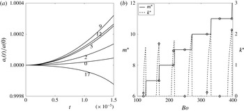
The most unstable wavenumbers were obtained from direct numerical time integration by generating curves similar to those in figure 3(a) for a range of values of
 $k$
and
 $m$
and identifying the pair
 $(k^{\ast },m^{\ast })$
for which
 $a(t)$
is maximum at some later time. Figure 4(a) is a plot of normalized amplitude versus time for a range of
 $m$
values at
 $Bo=250$
. At this condition, we expect the dominant mode to be the flute mode (
 $k^{\ast }=0$
). From the range of
 $m$
values considered, the curve corresponding to
 $m=9$
appears to grow to the highest amplitude. This indicates that
 $m^{\ast }=9$
at this
 $Bo$
. This procedure has been employed to search the
 $(k,m)$
space for the combination that yields the highest amplitude at several values of
 $Bo$
. These values of
 $(k^{\ast },m^{\ast })$
are shown as symbols in figure 4(b). As mentioned before, the analytical dispersion relation has been derived from (2.18) based on the frozen-flow approximation. The solid line in figure 4(b) represents the value of
 $m^{\ast }$
(which is an integer) and the dashed line represents the value of
 $k^{\ast }$
, both versus
 $Bo$
as obtained from the frozen-flow-based analytical dispersion relation (2.22). The discontinuous nature of
 $k^{\ast }$
in figure 4(b) is a result of mode switching between flute and helical modes (Vadivukkarasan & Panchagnula Reference Vadivukkarasan and Panchagnula2016). As can be seen, the analytical dispersion relation yields the same results as the exact numerically obtained values, indicating that the frozen-flow approximation is valid. We will henceforth only present the results obtained from the analytical equation (2.22).
(a) Plot of
 $a_{i}(t)/a_{i}(0)$
versus time for different values of
 $m$
. Here,
 $Bo=250$
,
 $Q_{i}=Q_{o}=10^{-3}$
,
 $We_{i}=We_{o}=0$
,
 $\unicode[STIX]{x1D6FC}=10^{-2}$
and
 $\unicode[STIX]{x1D706}=0.005$
. Note that the curve corresponding to
 $m=9$
increases faster than all other values of
 $m$
. Also, curves corresponding to all values of
 $k$
(not indicated in the panel) increase slower than
 $k=0$
. Therefore,
 $(k^{\ast },m^{\ast })=(0,9)$
for this case. (b) Plot of
 $k^{\ast }$
and
 $m^{\ast }$
versus
 $Bo$
. The continuous line represents the values obtained using the frozen-flow approximation and symbols ♢ and ○, respectively, indicate the values of
 $k^{\ast }$
and
 $m^{\ast }$
obtained from the direct numerical time integration. In this panel,
 $Q_{i}=Q_{o}=10^{-3}$
,
 $We_{i}=We_{o}=0$
,
 $\unicode[STIX]{x1D6FC}=10^{-2}$
and
 $\unicode[STIX]{x1D706}=0.005$
. The values obtained from the frozen-flow approximation agree well with those from direct numerical time integration.

Plot of amplitude growth rate (
 $\unicode[STIX]{x1D714}^{\ast }$
) versus pipe radius ratio (
 $\unicode[STIX]{x1D6FC}$
) for various values of
 $Bo$
. In this figure,
 $Q_{i}=Q_{o}=10^{-3}$
,
 $We_{i}=We_{o}=0$
and
 $\unicode[STIX]{x1D706}=0.98$
. The values of
 $\unicode[STIX]{x1D714}^{\ast }$
are independent of
 $\unicode[STIX]{x1D6FC}$
for
 $\unicode[STIX]{x1D6FC}<10^{-1}$
. We have chosen
 $\unicode[STIX]{x1D6FC}=10^{-3}$
for our calculations to ensure that the pipe radius plays no role.

2.7 Effect of
 $\unicode[STIX]{x1D6FC}$
on the instability characteristics

It may be recalled that the pipe from
 $0<r<R_{p}$
was a model introduced to induce radial motion at the two interfaces while overcoming the singularity. We wish to show that the specific value of
 $R_{p}$
(or
 $\unicode[STIX]{x1D6FC}$
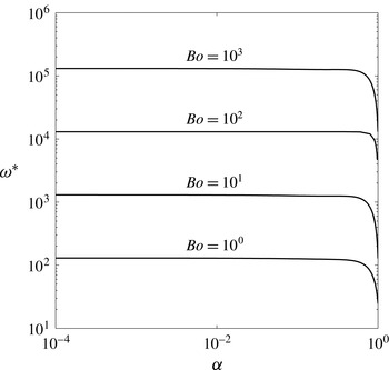
) does not play a significant role in determining the instability modes. Figure 5 shows the plot of dominant instability growth rate (
 $\unicode[STIX]{x1D714}^{\ast }$
) versus pipe radius ratio (
 $\unicode[STIX]{x1D6FC}$
) for four different values
 $Bo>0$
. For these values of
 $Bo$
, it can be observed that
 $\unicode[STIX]{x1D6FC}$
has an effect on
 $\unicode[STIX]{x1D714}^{\ast }$
only for
 $\unicode[STIX]{x1D6FC}>10^{-1}$
. For all the values of
 $\unicode[STIX]{x1D6FC}<10^{-1}$
and over three orders of magnitude variation in
 $Bo$
, the value of
 $\unicode[STIX]{x1D714}^{\ast }$
is independent of
 $\unicode[STIX]{x1D6FC}$
. Similar features can be observed for other parameters such as
 $k^{\ast }$
and
 $m^{\ast }$
associated with the instability. It is also observed that
 $\unicode[STIX]{x1D6FC}$
has a similar effect even for
 $Bo<0$
as well as for all values of non-zero inner and outer Weber numbers. In the present study, therefore,
 $\unicode[STIX]{x1D6FC}$
is taken to be
 $10^{-3}$
to ensure that all the results presented are independent of
 $\unicode[STIX]{x1D6FC}$
.
3 Special cases of the dispersion relation
Equation (2.22) is the dispersion relation governing the growth of three-dimensional instabilities due to the combined incidence of RT and KH mechanisms on an annular liquid sheet surrounded by gases at the two interfaces. We recover the dispersion relations previously published in the literature as special cases of (2.22). In recovering these special cases, we set
 $\unicode[STIX]{x1D6FC}\rightarrow 0$
.
The dispersion relation for axisymmetric (
 $m=0$
) capillary instability of an annular sheet (Meyer & Weihs Reference Meyer and Weihs1987) can be recovered from the present equation (2.22) by substituting
 $Bo=We_{i}=We_{o}=S=0$
. When
 $Bo=S=0$
, (2.22) reduces to the dispersion relation given by Panchagnula et al. (Reference Panchagnula, Sojka and Santangelo1996) for three-dimensional KH instability. When
 $R_{m}\rightarrow \infty$
with
 $(R_{o}-R_{i})$
being set to the sheet thickness and
 $m=0$
, the form of the dispersion relation of a planar liquid sheet subjected to KH mechanism can be recovered by neglecting viscous effects from the study of Li (Reference Li1994). On the same note, the results of Ibrahim & Akpan (Reference Ibrahim and Akpan1998) can be obtained if the surrounding gases are assumed as stationary in the present study. Furthermore, (2.22) also encompasses all the special cases discussed by Jeandel & Dumouchel (Reference Jeandel and Dumouchel1999) for the inviscid case.
The three-dimensional RT instability study of Velikovich & Schmit (Reference Velikovich and Schmit2015) can be obtained from (2.22) if
 $We_{i}=We_{o}=0$
. Likewise, the study of Mikaelian (Reference Mikaelian2005) can also be obtained if
 $k\rightarrow 0$
and
 $We_{i}=We_{o}=0$
. Both the single- and two-interface results can be recovered from (2.22) in the absence of surface tension acting at both interfaces. Moreover, the two-dimensional study of Chen et al. (Reference Chen, Schrock and Peterson1997) for a single interface can be obtained if
 $k\rightarrow 0$
and
 $We_{i}=We_{o}=0$
while
 $Q_{o}=1$
.
Finally, the dispersion relation for a single interface subjected to combined RT and KH mechanisms (Vadivukkarasan & Panchagnula Reference Vadivukkarasan and Panchagnula2016) can be recovered using one of the following two limits: (1)
 $Q_{i}=1$
and
 $We_{i}=0$
or (2)
 $Q_{o}=1$
and
 $We_{o}=0$
. In this way, the dispersion relation obtained from the present study (2.22) is more general than all the cases that have been published in the literature.
4 Results
This section presents the results pertaining to the behaviour of instabilities associated with combined RT and KH mechanisms acting on an annular liquid sheet. The overarching objective is to show that the dispersion relation developed in this work is able to identify the onset of different destabilization modes. Towards this end, it is of interest to understand the competition between radial acceleration forces and axial inertial forces. No assumptions have been made in deriving the dispersion relation with regard to the radius ratio (
 $\unicode[STIX]{x1D706}$
), which has two asymptotic limits – thick and thin. From the literature,
 $(R_{o}-R_{i})/R_{m}\sim 1$
is typically considered to imply a thick annular sheet, while
 $(R_{o}-R_{i})/R_{m}\ll 1$
typically implies that the sheet can be considered to be in the thin limit. Though (2.22) is capable of determining the destabilization characteristics in both the thick and thin limits, special attention will be devoted to the sheet in the thin limit by choosing
 $\unicode[STIX]{x1D706}=0.98$
for this study. We also choose
 $Q_{i}=Q_{o}=10^{-3}$
and
 $S=0$
for this study.
KH instability occurs as soon as the relative speed at an interface is non-zero (
 $We>0$
), irrespective of the values of
 $Q_{i}$
and
 $Q_{o}$
. On the other hand, RT instability only occurs when the fluids are unfavourably density-stratified, i.e. when the local acceleration field vector points from the heavier fluid to the lighter fluid. Extending this argument to multiple fluids separated by interfaces, even if one of the interfaces exhibits an unfavourable density stratification, the system is unstable. A note on the meaning of
 $\ddot{R}_{i}$
and
 $\ddot{R}_{o}$
is in order to reconcile these quantities with the usual gravitational acceleration-induced RT instability.
 $\ddot{R_{i}}$
is the instantaneous acceleration of the interface at current location
 $r=R_{i}$
. This acceleration is measured in the laboratory frame of reference. However, the equivalent local acceleration field due to the inertial force is in the opposite direction, from d’Alembert’s principle. Therefore, if
 $\ddot{R_{i}}>0$
, i.e. if the interface is moving outwards, the equivalent local radial acceleration field due to the inertial force experienced by the fluids is radially inwards. Therefore, an unstable density stratification at this interface would imply that
 $\unicode[STIX]{x1D70C}_{l}$
has to be greater than
 $\unicode[STIX]{x1D70C}_{i}$
, or
 $Q_{i}<1$
, otherwise the system would be unconditionally stable as far as RT instability is concerned.
Now let us consider the case of an annular liquid sheet with two interfaces separating three fluids. The system is stable if both interfaces show favourable density stratification. For an annular sheet, this criterion also involves the disturbance mode,
 $m$
(Mikaelian Reference Mikaelian2005). Mathematically, if
 $[1-m(1-Q_{i})]\ddot{R_{i}}>0$
and
 $[1+m(1-Q_{o})]\ddot{R_{o}}>0$
, then the system is stable. The system is unstable if any of the conditions for stability given above are violated, i.e. if either
 $[1-m(1-Q_{i})]\ddot{R_{i}}<0$
or
 $[1+m(1-Q_{o})]\ddot{R_{o}}<0$
, an unfavourable density stratification will lead to exponential instability. We are primarily interested in the latter cases, since they are relevant to primary atomization.
The case where the fluids are stably stratified with
 $We_{i}=We_{o}=0$
is also interesting in its own right. In order to understand the physics associated with this stability, let us first consider the case where
 $\ddot{R_{i}}=\ddot{R_{o}}=0$
. Under this condition, the dispersion relation (2.22) gives rise to purely imaginary eigenvalues, i.e. any imposed perturbation will not decay in amplitude, but will exhibit periodic oscillations. Therefore, strictly speaking, this system is neutrally stable. The RT stability behaviour of this system is analogous to the oscillations of a pendulum with time-varying length (Sánchez-Soto & Zoido Reference Sánchez-Soto and Zoido2013). Then
 $R_{i}$
takes on the role of the length of the pendulum and
 ${\dot{R}}_{i}>0$
would imply an oscillating pendulum whose length is increasing. Analogously, if the system is neutrally stable and if
 ${\dot{R}}_{i}>0$
, oscillations imposed on the system would decay, but not exponentially (Roman, Gay & Clanet Reference Roman, Gay and Clanet2001). If
 ${\dot{R}}_{i}<0$
, the oscillations would increase in amplitude but (again) not exponentially.
In this study, we are specifically interested in the onset of instability via three-dimensional modes since they are likely to yield a shorter characteristic length scale,
 ${\mathcal{L}}^{\ast }$
(defined earlier in (2.23)). We will show that, under these conditions of
 $Bo$
,
 $We_{i}$
and
 $We_{o}$
, three-dimensional modes are preferred by the system in comparison to two-dimensional instability modes. Before considering the general case, it will be beneficial to briefly investigate the destabilization behaviour due to KH and RT mechanisms occurring separately.
4.1 Pure Kelvin–Helmholtz instability and pure Rayleigh–Taylor instability
The role of each instability mechanism (RT or KH) on an annular liquid sheet will be discussed briefly. We begin with KH instability. In order to study the influence of the KH mechanism (unequal axial velocities) on the annular sheet, we set
 $Bo=0$
in (2.22). The influence of inner (
 $We_{i}$
) and outer (
 $We_{o}$
) Weber numbers on the characteristic length scale (
 ${\mathcal{L}}^{\ast }$
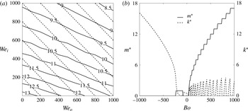
) will be discussed using figure 6(a) for pure KH instability. Figure 6(a) shows contours of constant
 ${\mathcal{L}}^{\ast }$
as a function of
 $We_{i}$
and
 $We_{o}$
. The dashed lines in figure 6(a) represent lines of constant energy (
 $\unicode[STIX]{x1D701}$
) where
 $\unicode[STIX]{x1D701}=We_{i}+We_{o}$
. It can be seen that
 $\unicode[STIX]{x1D701}$
is the total kinetic energy per unit volume in the inner and outer air streams measured in units of
 $\unicode[STIX]{x1D70E}/R_{m}$
. For a given
 $\unicode[STIX]{x1D701}$
, it would be interesting to identify the parametric condition that yields a minimum in characteristic length scale. It can be seen that
 ${\mathcal{L}}^{\ast }$
decreases with increasing
 $We_{i}$
,
 $We_{o}$
or
 $\unicode[STIX]{x1D701}$
. The decrease is also nonlinear for high
 $\unicode[STIX]{x1D701}$
. Finally, the minimum
 $\unicode[STIX]{x1D701}$
required to achieve a given
 ${\mathcal{L}}^{\ast }$
occurs at
 $We_{o}=0$
. This is similar to the conclusion of Liao et al. (Reference Liao, Jeng, Jog and Benjamin2000) from their work on annular liquid sheets. In addition, it is observed that, for the range of parameters considered herein, the annular sheet is susceptible only to axisymmetric modes (referred to as Taylor mode in this study).
(a) Contour plot showing lines of constant characteristic instability length scale,
 ${\mathcal{L}}^{\ast }$
, in the
 $We_{i}$
–
 $We_{o}$
plane for
 $Bo=0$
,
 $Q_{i}=Q_{o}=10^{-3}$
and
 $\unicode[STIX]{x1D706}=0.98$
(pure KH instability). The dashed lines represent lines of constant dimensionless energy
 $\unicode[STIX]{x1D701}$
where
 $We_{i}+We_{o}=\unicode[STIX]{x1D701}$
. The
 $\unicode[STIX]{x1D701}$
value is allowed to vary from
 $200$
to
 $1800$
in steps of
 $200$
. On any line of constant
 $\unicode[STIX]{x1D701}$
,
 ${\mathcal{L}}^{\ast }$
is minimum when
 $We_{o}=0$
. (b) Plot of
 $m^{\ast }$
and
 $k^{\ast }$
versus Bond number. Here,
 $We_{i}=We_{o}=0$
,
 $Q_{i}=Q_{o}=10^{-3}$
and
 $\unicode[STIX]{x1D706}=0.98$
. The solid line represents
 $m^{\ast }$
and the dashed line represents
 $k^{\ast }$
. For
 $Bo<0$
,
 $k^{\ast }$
increases with increasing
 $|Bo|$
and for
 $Bo>0$
,
 $m^{\ast }$
generally increases with increasing
 $|Bo|$
, while
 $k^{\ast }$
shows mode switching between flute and helical modes.

We now move on to discussing the effect of RT instability occurring alone by setting
 $We_{i}=We_{o}=0$
in (2.22). Figure 6(b) presents a plot of the most unstable wavenumbers (
 $k^{\ast },m^{\ast }$
) as a function of Bond number (
 $Bo$
). The occurrence of such destabilization modes can be observed in figure 6(b). Let us first consider the case where
 $Bo<0$
. It can be observed that
 $k^{\ast }$
increases with increasing
 $|Bo|$
for
 $-200\lessapprox Bo<0$
, while
 $m^{\ast }$
is either
 $0$
or
 $1$
. These correspond to either Taylor or sinuous mode (
 $k^{\ast }>0,m^{\ast }=1$
). Further increase in
 $|Bo|$
(i.e.
 $\lessapprox -200$
) causes the most unstable wavenumber pair to shift back to Taylor mode. As figure 6(b) indicates,
 $k^{\ast }$
increases as
 $|Bo|$
increases for
 $Bo\lessapprox -200$
.
Let us now consider the case where
 $Bo>0$
in figure 6(b). The existence of three-dimensional modes where
 $k^{\ast }$
and
 $m^{\ast }$
are both non-zero can be observed here. With an increase in
 $Bo$
, the instability mode shifts from the Taylor mode to three-dimensional (helical) modes or switches between flute and helical modes. The physics associated with this mode switching has been discussed in Vadivukkarasan & Panchagnula (Reference Vadivukkarasan and Panchagnula2016) and the reader is referred to that work for more details. One possible hypothesis that could explain the difference in behaviour between negative and positive
 $Bo$
is as follows. For a liquid sheet undergoing outward radial acceleration (negative
 $Bo$
), surface tension force and the d’Alembert force due to radial acceleration act in the same direction. In contrast, when the sheet is subjected to inward radial acceleration (positive
 $Bo$
), surface tension force and the d’Alembert force act in opposite directions, causing further destabilization. While any
 $Bo$
(positive or negative) causes instability,
 $Bo>0$
results in the manifestation of helical modes. Another significant conclusion from figure 6(b) is that, for large
 $|Bo|$
, the curves for
 $k^{\ast }$
for
 $Bo<0$
and
 $m^{\ast }$
for
 $Bo>0$
are nearly symmetric even though the destabilization modes are different.
4.2 Combined Rayleigh–Taylor and Kelvin–Helmholtz mechanisms
We will now discuss the results associated with the combined occurrence of both RT and KH mechanisms. These results fall into three categories: (1) regime map showing the parametric classification of different modes; (2) neutral stability plots and most unstable wavenumbers; and (3) energy budget analysis to describe the optimal partitioning of energy to achieve a minimum instability length scale.
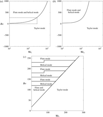
Regime map for the combined RT and KH instability case showing the occurrence of various destabilization modes in different planes. (a) Bond number (
 $Bo$
) versus inner Weber number (
 $We_{i}$
) plane. Here,
 $We_{o}=0$
and
 $Q_{j}=10^{-3}$
. The line separating Taylor mode from other modes is given by the approximate equation
 $Bo\approx We_{i}$
. (b) Bond number (
 $Bo$
) versus outer Weber number (
 $We_{o}$
) plane. Here,
 $We_{i}=0$
and
 $Q_{j}=10^{-3}$
. The line separating Taylor mode from other modes is given by the approximate equation
 $Bo\approx We_{o}/4$
. (c) Magnified view of the region inside the dashed rectangle in panel (a). Banded nature showing alternating flute and helical modes can be observed in panel (c). High values of
 $We$
always result in the occurrence of axisymmetric Taylor mode.

4.2.1 Regime map in
$Bo$
and
$We$
space


A regime map depicting the occurrence of the three different destabilization modes is constructed in the (
 $Bo$
,
 $We_{i}$
,
 $We_{o}$
) space and presented in figure 7. Note that the ordinate is linear, while the abscissa is on a logarithmic scale in figure 7(a,b). The parameter space is divided into three regimes: (1) the Taylor mode, (2) the flute mode and (3) the helical mode. It can be observed from figure 7(a) that the parameter space where the Taylor mode is manifest is clearly identified. For a given
 $We_{i}$
, one observes a transition from the Taylor mode to the flute and the helical mode at a critical positive value of
 $Bo$
. The critical value is related to
 $We_{i}$
by the approximate equation
 $Bo\approx We_{i}$
. Beyond this value of
 $Bo$
, the system is unstable to helical and flute modes. To understand the flute and the helical mode regimes, consider figure 7(c), which is a magnified view of the region of the regime plot in figure 7(a) for
 $0<Bo<250$
and
 $0<We<300$
. It can be observed from figure 7(c) that the instability modes alternate between flute and helical modes as
 $Bo$
increases. A similar banded structure was previously discussed in the context of the RT mechanism when figure 6(b) was discussed in the context of
 $Bo>0$
. Figure 7(b) is similar to figure 7(a) except that
 $We_{o}$
is considered in place of
 $We_{i}$
. Note that the transition from the Taylor mode to the flute and the helical mode at a critical positive value of
 $Bo$
for a given
 $We_{o}$
is different from that in figure 7(a). This critical value is now given by
 $Bo\approx We_{o}/4$
.
4.2.2 Neutral stability plots and most unstable wavenumbers
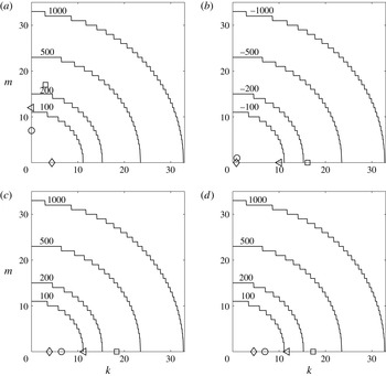
Plots of neutral stability curves in the
 $(k,m)$
plane separating the stable and unstable regions. The region of the
 $(k,m)$
plane that includes the origin is the stable region. Plots are shown for various values of
 $Bo$
,
 $We_{i}$
and
 $We_{o}$
. Here,
 $Q_{i}=Q_{o}=10^{-3}$
and
 $\unicode[STIX]{x1D706}=0.98$
. The stepwise variation observed in the neutral stability curves is due to the integer values of the circumferential wavenumber. The four curves are for: (a)
 $Bo=100$
,
 $200$
,
 $500$
and
 $1000$
,
 $We_{i}=100$
and
 $We_{o}=0$
; (b)
 $Bo=-100$
,
 $-200$
,
 $-500$
and
 $-1000$
,
 $We_{i}=100$
and
 $We_{o}=0$
; (c)
 $Bo=100$
,
 $200$
,
 $500$
and
 $1000$
,
 $We_{i}=1000$
and
 $We_{o}=0$
; (d)
 $Bo=100$
,
 $200$
,
 $500$
and
 $1000$
,
 $We_{i}=0$
and
 $We_{o}=1000$
. In these panels
 $(k^{\ast },m^{\ast })$
corresponding to each
 $Bo$
is indicated using symbols. The value of
 $|Bo|$
corresponding to each symbol is as follows: ♢,
 $100$
; ○,
 $200$
; ◃,
 $500$
; and ▫,
 $1000$
. The neutral stability boundary is influenced mainly by
 $Bo$
and is weakly dependent on
 $We_{i}$
or
 $We_{o}$
. However,
 $We_{i}$
and
 $We_{o}$
determine
 $(k^{\ast },m^{\ast })$
. It can also be observed that
 $k_{c}\approx m_{c}$
in all cases.

We now turn our attention to neutral stability curves, which are curves in the wavenumber space
 $(k,m)$
separating the stable and unstable regions. Figure 8 shows the neutral stability curves for a set of
 $|Bo|$
,
 $We_{i}$
and
 $We_{o}$
values. Figures 8(a)–8(d) each corresponds to one set of Weber number values (
 $We_{i}$
or
 $We_{o}$
) and contains the neutral stability curves for four values of Bond number,
 $|Bo|=100$
,
 $200$
,
 $500$
and
 $1000$
, with the values indicated on the respective curves. The location of
 $(k^{\ast },m^{\ast })$
is indicated by symbols as mentioned in the caption.
Figure 8(a) presents the neutral stability plot for
 $Bo>0$
and
 $We_{i}=100$
with
 $We_{o}=0$
. The stepwise behaviour is due to the fact that
 $m$
takes on only integer values. It can be observed from figure 8(a) that
 $Bo$
has a significant effect on determining the neutral stability curve. An increase in
 $Bo$
increases the range of unstable wavenumbers (
 $k,m$
) and causes the neutral stability curve to move outwards in both axial and circumferential directions. In addition, both the dimensionless cutoff axial wavenumber (
 $k_{c}$
) and cutoff circumferential wavenumber (
 $m_{c}$
) increase as the Bond number increases. The points corresponding to (
 $k^{\ast },m^{\ast }$
) are indicated by symbols. It can be concluded that the fluid interface is unstable to two-dimensional modes as well as to three-dimensional modes under these conditions. The Taylor mode is observed for
 $Bo=100$
while the flute mode is observed for
 $Bo=200$
and
 $500$
. For
 $Bo=1000$
, both
 $k^{\ast }$
and
 $m^{\ast }$
are non-zero, indicating the occurrence of the helical mode. It can be observed from figure 8(a) that both two- and three-dimensional modes are manifest due to the combined action of both mechanisms. This observation is significant, as three-dimensional modes could give rise to shorter length scales on the fluid interface (Panchagnula et al.
Reference Panchagnula, Sojka and Santangelo1996). We will revisit this later when we discuss the parametric conditions when such three-dimensional modes can be observed.
Figure 8(b) is similar to figure 8(a) except that the values of
 $Bo$
are negative. Still,
 $We_{i}=100$
and
 $We_{o}=0$
. The neutral stability curves for
 $Bo<0$
(figure 8
b) are nearly identical to those for
 $Bo>0$
(figure 8
a) for the same
 $|Bo|$
. This implies that the direction of radial acceleration has no influence in determining the neutral stability region. However, the sign change has a marked effect on determining the most unstable wavenumbers. The sinuous mode is now observed for
 $Bo=-200$
, while Taylor modes are observed for
 $Bo=-100$
,
 $-500$
and
 $-1000$
.
Figure 8(c,d) presents the neutral stability plots for
 $Bo>0$
for (
 $We_{i},We_{o}$
) = (
 $1000,0$
) and (
 $0,1000$
), respectively. The neutral stability curves in figure 8(c,d) are similar to those in figure 8(a). This implies that Weber numbers play an insignificant role in determining the neutral stability region. However, the most unstable wavenumber pair (
 $k^{\ast },m^{\ast }$
) is different when both RT and KH mechanisms play a role. It can be observed from figure 8(a) that
 $Bo=1000$
and
 $We_{i}=1000$
and
 $We_{o}=0$
yields three-dimensional modes. However, for the same
 $Bo$
, the inclusion of
 $We_{i}$
or
 $We_{o}$
yields only two-dimensional axisymmetric modes. Increasing either
 $We_{i}$
or
 $We_{o}$
is actually found to be counterproductive, because the instability mode switches back to Taylor mode from a non-axisymmetric mode. Finally, the neutral stability curves (figure 8
a–d) show that
 $k_{c}\approx m_{c}$
for all values of
 $Bo$
,
 $We_{i}$
and
 $We_{o}$
considered in this study, with
 $k_{c}$
and
 $m_{c}$
being functions of only
 $|Bo|$
.
4.3 Energy budget analysis
Linear instability analysis predicts the most unstable wavenumber pair for a given flow condition. It can also be used to estimate an optimal parameter set for which the interface distortion length scale is minimum. In this section, we will devote our attention to finding an optimal parameter value set, (
 $Bo$
,
 $We_{i}$
,
 $We_{o}$
), such that
 ${\mathcal{L}}^{\ast }$
is minimized. We will perform this optimization subject to the constraint that the total energy is constant. The motivation for this effort is to find the optimal partitioning of energy between radial acceleration and velocity shear in order to achieve efficient atomization. For this purpose, a total energy parameter, given by
 $\unicode[STIX]{x1D716}=(\unicode[STIX]{x1D70C}_{i}-\unicode[STIX]{x1D70C}_{l})R\ddot{R}+\unicode[STIX]{x1D70C}_{l}(W_{l}-W_{i})^{2}+\unicode[STIX]{x1D70C}_{l}(W_{l}-W_{o})^{2}$
is defined. Here,
 $\unicode[STIX]{x1D716}$
is a measure of the total energy available in the mean flow due to the acceleration field (first term) and in the form of relative kinetic energy in the two streams (second and third terms). Incidentally,
 $R_{m}\unicode[STIX]{x1D716}/\unicode[STIX]{x1D70E}=|Bo|+We_{i}+We_{o}=\unicode[STIX]{x1D701}$
(say).
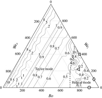
A ternary phase diagram showing contours of constant
 ${\mathcal{L}}^{\ast }$
as a function of
 $(Bo,We_{i},We_{o})$
. The three sides of the triangle of the regime map correspond to the Bond number (
 $Bo$
), inner Weber number (
 $We_{i}$
) and outer Weber number (
 $We_{o}$
). For all points in this figure,
 $\unicode[STIX]{x1D701}=Bo+We_{i}+We_{o}=1000$
. The solid lines indicate contours of constant values of
 ${\mathcal{L}}^{\ast }$
. A dashed line separates the Taylor mode regime and the helical mode. The symbol ○ denotes the global minimum characteristic length scale (
 ${\mathcal{L}}^{\ast }\approx 0.08$
) for this value of
 $\unicode[STIX]{x1D701}$
. We have
 $(Bo,We_{i},We_{o})=(900,0,100)$
for ○. Other local minima corresponding to
 ${\mathcal{L}}^{\ast }\approx 0.1$
occur at the following flow conditions: ▫, (
 $600,400,0$
); ◃, (
 $680,220,100$
); and ♢, (
 $900,100,0$
). All minima occur only in the helical mode regime.

Since the optimization is being performed in a three-dimensional parameter space (
 $Bo,We_{i},We_{o}$
), subject to
 $\unicode[STIX]{x1D701}$
being constant, we find it useful to represent the data in the form of a ternary phase diagram. Figure 9 shows such a phase diagram. Every point inside the ternary diagram is represented by the three coordinates,
 $Bo$
,
 $We_{i}$
and
 $We_{o}$
, such that
 $Bo+We_{i}+We_{o}=\unicode[STIX]{x1D701}=1000$
. Only positive values of
 $Bo$
are considered herein, as they have been shown to give rise to helical modes (see e.g. figure 6
b). A dashed line is indicated separating regions where the Taylor mode is manifest from regions where helical and flute modes dominate. As can be seen, higher values of
 $Bo$
tend to give rise to helical modes, which are beneficial to atomization. Figure 9 also shows contours of
 ${\mathcal{L}}^{\ast }$
in the three-parameter space. Firstly, it can be observed that, for low values of
 $Bo$
(
 ${<}400$
), these lines of constant
 ${\mathcal{L}}^{\ast }$
are parallel to the
 $We_{o}$
axis, which are lines of constant
 $Bo$
. This implies that, for
 $Bo<400$
,
 ${\mathcal{L}}^{\ast }$
is a function of
 $Bo$
only and is relatively insensitive to both
 $We_{o}$
and
 $We_{i}$
. In addition, as
 $Bo$
increases,
 ${\mathcal{L}}^{\ast }$
monotonically decreases.
As
 $Bo$
increases further, the lines of constant
 ${\mathcal{L}}^{\ast }$
are no longer parallel to lines of constant
 $Bo$
, indicating the effect of combining RT and KH mechanisms. In the bottom right corner of figure 9, the lines of constant
 ${\mathcal{L}}^{\ast }$
show significant non-monotonic behaviour. For
 $\unicode[STIX]{x1D701}=1000$
(as has been chosen for figure 9), the global minimum value of
 ${\mathcal{L}}^{\ast }$
(
 ${\approx}0.08$
) occurs at
 $(Bo,We_{i},We_{o})\approxeq (900,0,100)$
. This point is indicated by the circle in figure 9. Several local minima are also indicated by other symbols. The values of
 ${\mathcal{L}}^{\ast }$
associated with these minima are reported in the caption. The relative proportion of
 $Bo$
to
 $We_{o}$
at these points suggests an optimal partitioning of energy. It appears that
 $90\,\%$
of
 $\unicode[STIX]{x1D701}$
being used to induce radial acceleration with the remaining
 $10\,\%$
being used to create relative motion in the outer air stream yields a minimum value of
 ${\mathcal{L}}^{\ast }$
. When
 $Bo=0$
, we found from figure 6(a) that the optimal mode will occur when all the energy is concentrated in
 $We_{i}$
. However, in the case of RT–KH instability, the optimal mode occurs when most of the energy is concentrated in
 $Bo$
. Numerically, the values of
 ${\mathcal{L}}^{\ast }$
in figure 9 for
 $(Bo,We_{i},We_{o})=(900,0,100)$
and
 $(Bo,We_{i},We_{o})=(900,100,0)$
are close. Hence, the only reliable conclusion that can be drawn from figure 9 is that radial acceleration is significantly more important in causing destabilization than any axial motion.
Plot of minimum characteristic length scale (
 ${\mathcal{L}}_{m}^{\ast }$
) versus
 $\unicode[STIX]{x1D701}$
. The symbols ○ and ♢ indicate the values of
 ${\mathcal{L}}_{m}^{\ast }$
obtained from the combined action of RT and KH mechanisms; ○ and ♢ correspond to
 $Bo>0$
and
 $Bo<0$
, respectively; and ▫ corresponds to
 $Bo=0$
representing the KH instability mechanism acting alone. For
 $\unicode[STIX]{x1D701}>200$
,
 ${\mathcal{L}}_{m}^{\ast }\sim \unicode[STIX]{x1D701}^{-3/5}$
for both
 $Bo>0$
and
 $Bo<0$
cases. Combining the RT and KH mechanisms of instability yields a lower
 ${\mathcal{L}}_{m}^{\ast }$
than pure KH instability when
 $\unicode[STIX]{x1D701}>200$
.

For each value of
 $\unicode[STIX]{x1D701}$
, an optimal parameter value set can be identified and the corresponding value of minimum
 ${\mathcal{L}}^{\ast }$
can be noted from a plot similar to figure 9. We now turn our attention to understanding the variation of the global minimum
 ${\mathcal{L}}^{\ast }$
(referred to as
 ${\mathcal{L}}_{m}^{\ast }$
) as a function of
 $\unicode[STIX]{x1D701}$
. Figure 10 is a plot of
 ${\mathcal{L}}_{m}^{\ast }$
versus
 $\unicode[STIX]{x1D701}$
for cases where both the RT and KH mechanisms are active. For reference, we have also indicated the values of
 ${\mathcal{L}}_{m}^{\ast }$
for the KH mechanism alone (
 $Bo=0$
). When the KH mechanism alone is active, the optimal parameter configuration always occurs when
 $We_{i}=\unicode[STIX]{x1D701}$
and
 $We_{o}=0$
. This is consistent with the findings of Shen & Li (Reference Shen and Li1996) and Liao et al. (Reference Liao, Jeng, Jog and Benjamin2000) as well as with the data presented in figure 6(a).
Three trends can be observed from figure 10. Firstly, for
 $\unicode[STIX]{x1D701}<40$
, all three cases (
 $Bo>0$
,
 $Bo<0$
and
 $Bo=0$
) show similar values of
 ${\mathcal{L}}_{m}^{\ast }$
. This implies that radial acceleration-induced destabilization is not helpful at such low dimensionless energy values. In contrast, for
 $\unicode[STIX]{x1D701}>200$
, the cases with both
 $Bo>0$
and
 $Bo<0$
appear to yield markedly lower values of
 ${\mathcal{L}}_{m}^{\ast }$
than the case without radial acceleration (
 $Bo=0$
). In addition, for
 $\unicode[STIX]{x1D701}>200$
,
 ${\mathcal{L}}_{m}^{\ast }\sim \unicode[STIX]{x1D701}^{-3/5}$
. For such large values of
 $\unicode[STIX]{x1D701}$
, the optimal parameter values of
 $Bo$
,
 $We_{i}$
and
 $We_{o}$
indicate that a significant fraction of the total energy should be focused on radial acceleration (similar to the conclusion related to figure 9). For
 $40<\unicode[STIX]{x1D701}<200$
and
 $Bo<0$
, the system manifests the sinuous mode of instability with
 $(k^{\ast },m^{\ast })=(0,1)$
indicating a very high value of
 ${\mathcal{L}}_{m}^{\ast }$
and has not been shown in figure 10. However, for
 $Bo>0$
, the data are shown in figure 10. For this case, the results indicate a continuous decrease of
 ${\mathcal{L}}_{m}^{\ast }$
with increasing
 $\unicode[STIX]{x1D701}$
. It can also be observed that, for
 $\unicode[STIX]{x1D701}>200$
, the values of
 ${\mathcal{L}}_{m}^{\ast }$
governing destabilization decrease more steeply for both the
 $Bo\neq 0$
cases than for the
 $Bo=0$
case. From data in figure 10, one can calculate the power-law exponent for the variation of
 ${\mathcal{L}}_{m}^{\ast }$
with
 $\unicode[STIX]{x1D701}$
(for
 $\unicode[STIX]{x1D701}>200$
). For the combined RT and KH mechanisms on an annular liquid sheet (for both
 $Bo<0$
as well as
 $Bo>0$
), we show that
 ${\mathcal{L}}_{m}^{\ast }\sim \unicode[STIX]{x1D701}^{-3/5}$
. For the case of a single cylindrical interface, Vadivukkarasan & Panchagnula (Reference Vadivukkarasan and Panchagnula2016) have shown that
 ${\mathcal{L}}_{m}^{\ast }\sim \unicode[STIX]{x1D701}^{-1/2}$
. In addition, it can be seen from figure 10 that
 ${\mathcal{L}}_{m}^{\ast }$
for pure KH instability is at least an order of magnitude higher. This effect quantifies the benefits associated with invoking RT instability as a primary source of destabilization in atomizers. Therefore, it can concluded from figure 10 that high-energy atomization involving
 $\unicode[STIX]{x1D701}>200$
could yield disproportionate benefits if the atomizer is designed to work in the radial acceleration-induced instability mode.
5 Conclusion
An overarching objective of this study is to propose a new model for liquid atomization by emphasizing the advantages derived from accommodating radial acceleration along with axial motion to destabilize the annular liquid sheet. A temporal linear stability analysis is employed to study the stability characteristics of an annular liquid sheet under the simultaneous action of both RT and KH instability mechanisms occurring simultaneously. Using this analysis, the effect of various parameters on the most unstable wavenumbers has been studied.
The fluids in this study were considered to be immiscible, incompressible and inviscid, and the annular liquid sheet was subjected to three-dimensional disturbances. An analytical dispersion relation was obtained using the frozen-flow approximation. This has been shown to be more general than all the cases that have been published in the literature. The dispersion relation has been validated using the results obtained from direct numerical time integration of the linearized equations, without the frozen-flow assumption. The destabilization behaviour was observed to be governed by dimensionless quantities such as (1) Bond number based on radial acceleration (
 $Bo$
), (2) Weber numbers at the two interfaces based on the relative velocities (
 $We_{i}$
and
 $We_{o}$
) and (3) density ratios (
 $Q_{i}$
and
 $Q_{o}$
).
The destabilization characteristics due to the KH mechanism were found to be consistent with those from the existing literature. Depending upon the value of
 $Bo$
, the system was shown to manifest one of the following four modes of destabilization: (1) Taylor mode, which is axisymmetric two-dimensional; (2) flute mode, which is two-dimensional and longitudinal; (3) helical mode, which is three-dimensional; and (4) sinuous mode, which is a special case of the helical mode with one helix. Under certain parameter conditions, the interface was shown to be susceptible to three-dimensional long-wavelength helical modes. It was also shown that the increase in absolute value of Bond number causes an increase in the values of the most unstable wavenumbers, thereby decreasing the characteristic length scale associated with the instability.
The effect of
 $Bo$
as well as
 $We_{i}$
and
 $We_{o}$
on the destabilization characteristics has been quantified for a range of parameter values. It was observed that
 $Bo$
was a key determining parameter of the neutral stability region. It was also observed that the neutral stability curves are relatively insensitive to Weber numbers, but they play a significant role in determining the most unstable wavenumbers and instability mode choice. From the neutral stability plots, it was shown that the system is susceptible to three-dimensional long-axial-wavelength helical modes under certain parametric conditions. A regime map of the instability modes in
 $Bo$
,
 $We_{i}$
and
 $We_{o}$
space was also presented. From this regime map, it was shown that high
 $Bo$
and low
 $We_{i}$
(and
 $We_{o}$
) causes the atomization length scale to be reduced.
An energy budget analysis was presented for different values of constant total energy in a three-dimensional parameter space consisting of
 $Bo$
,
 $We_{i}$
and
 $We_{o}$
. It was observed that focusing the non-dimensional energy on radial acceleration yields minimum instability length scale compared with axial motion for the same energy. Finally, we show that, for high dimensionless energy (
 $\unicode[STIX]{x1D701}>200$
), the characteristic length scale (
 ${\mathcal{L}}_{m}^{\ast }$
) governing destabilization decreases as
 $\unicode[STIX]{x1D701}^{-3/5}$
. A clear case for utilizing the role of radial acceleration to destabilize annular liquid sheets has been made. These observations point towards new paradigms for designing atomizers using radial motion.
Appendix A
The system of linear equations obtained from combined action of the RT and KH instability mechanisms of an annular sheet can be written in the form of
 $[\unicode[STIX]{x1D63C}]_{7\times 7}[\boldsymbol{X}]_{7\times 1}=0$
, where
 $\unicode[STIX]{x1D63C}$
is given below and
 $[\boldsymbol{X}]^{\text{T}}=[{\mathcal{A}}_{i},{\mathcal{B}}_{i},{\mathcal{B}}_{o},{\mathcal{A}}_{l},{\mathcal{B}}_{l},a_{i},a_{o}]$
:
 $$\begin{eqnarray}\displaystyle & \displaystyle \unicode[STIX]{x1D63C}=\left(\begin{array}{@{}ccccccc@{}}-\overline{k}\text{I}_{m}^{\prime }(\overline{k}R_{i}) & \overline{k}\text{K}_{m}^{\prime }(\overline{k}R_{i}) & 0 & 0 & 0 & \unicode[STIX]{x1D608}_{16} & 0\\ \overline{k}\text{I}_{m}^{\prime }(\overline{k}R_{p}) & -\overline{k}\text{K}_{m}^{\prime }(\overline{k}R_{p}) & 0 & 0 & 0 & 0 & 0\\ 0 & 0 & \overline{k}\text{K}_{m}^{\prime }(\overline{k}R_{o}) & 0 & 0 & 0 & \unicode[STIX]{x1D608}_{37}\\ 0 & 0 & 0 & -\overline{k}\text{I}_{m}^{\prime }(\overline{k}R_{i}) & \overline{k}\text{K}_{m}^{\prime }(\overline{k}R_{i}) & \unicode[STIX]{x1D608}_{46} & 0\\ 0 & 0 & 0 & -\overline{k}\text{I}_{m}^{\prime }(\overline{k}R_{o}) & \overline{k}\text{K}_{m}^{\prime }(\overline{k}R_{o}) & 0 & \unicode[STIX]{x1D608}_{57}\\ \unicode[STIX]{x1D608}_{61} & 0 & 0 & \unicode[STIX]{x1D608}_{64} & \unicode[STIX]{x1D608}_{65} & \unicode[STIX]{x1D608}_{66} & 0\\ 0 & 0 & \unicode[STIX]{x1D608}_{73} & \unicode[STIX]{x1D608}_{74} & \unicode[STIX]{x1D608}_{75} & 0 & \unicode[STIX]{x1D608}_{77}\end{array}\right), & \displaystyle \nonumber\\ \displaystyle & & \displaystyle\end{eqnarray}$$
 $$\begin{eqnarray}\displaystyle & \displaystyle \unicode[STIX]{x1D608}_{16}=\overline{\unicode[STIX]{x1D714}}+\text{i}\overline{k}W_{i}+\frac{{\dot{R}}_{i}}{R_{i}}, & \displaystyle\end{eqnarray}$$
 $$\begin{eqnarray}\displaystyle & \displaystyle \unicode[STIX]{x1D608}_{37}=\overline{\unicode[STIX]{x1D714}}+\text{i}\overline{k}W_{o}+\frac{\dot{R_{o}}}{R_{o}}, & \displaystyle\end{eqnarray}$$
 $$\begin{eqnarray}\displaystyle & \displaystyle \unicode[STIX]{x1D608}_{46}=\overline{\unicode[STIX]{x1D714}}+\text{i}\overline{k}W_{l}+\frac{{\dot{R}}_{i}}{R_{i}}, & \displaystyle\end{eqnarray}$$
 $$\begin{eqnarray}\displaystyle & \displaystyle \unicode[STIX]{x1D608}_{57}=\overline{\unicode[STIX]{x1D714}}+\text{i}\overline{k}W_{l}+\frac{\dot{R_{o}}}{R_{o}}, & \displaystyle\end{eqnarray}$$
 $$\begin{eqnarray}\displaystyle & \displaystyle \unicode[STIX]{x1D608}_{61}=-\unicode[STIX]{x1D70C}_{i}((\overline{\unicode[STIX]{x1D714}}+\text{i}\overline{k}W_{1})\text{I}_{m}(\overline{k}R_{i})-{\dot{R}}_{i}\unicode[STIX]{x1D608}_{11}), & \displaystyle\end{eqnarray}$$
 $$\begin{eqnarray}\displaystyle & \displaystyle \unicode[STIX]{x1D608}_{64}=-\unicode[STIX]{x1D70C}_{l}((\overline{\unicode[STIX]{x1D714}}+\text{i}\overline{k}W_{l})\text{I}_{m}(\overline{k}R_{i})-{\dot{R}}_{i}\unicode[STIX]{x1D608}_{11}), & \displaystyle\end{eqnarray}$$
 $$\begin{eqnarray}\displaystyle & \displaystyle \unicode[STIX]{x1D608}_{65}=-\unicode[STIX]{x1D70C}_{l}((\overline{\unicode[STIX]{x1D714}}+\text{i}\overline{k}W_{l})\text{I}_{m}(\overline{k}R_{i})+{\dot{R}}_{i}\unicode[STIX]{x1D608}_{12}), & \displaystyle\end{eqnarray}$$
 $$\begin{eqnarray}\displaystyle & \displaystyle \unicode[STIX]{x1D608}_{66}=(\unicode[STIX]{x1D70C}_{i}-\unicode[STIX]{x1D70C}_{1})\ddot{R_{i}}-\frac{\unicode[STIX]{x1D70E}_{i}}{R_{i}^{2}}(1-m^{2}-\overline{k}^{2}R_{i}^{2}), & \displaystyle\end{eqnarray}$$
 $$\begin{eqnarray}\displaystyle & \displaystyle \unicode[STIX]{x1D608}_{73}=\unicode[STIX]{x1D70C}_{o}((\overline{\unicode[STIX]{x1D714}}+\text{i}\overline{k}W_{o})\text{K}_{m}(\overline{k}R_{o})-{\dot{R}}_{o}\unicode[STIX]{x1D608}_{33}), & \displaystyle\end{eqnarray}$$
 $$\begin{eqnarray}\displaystyle & \displaystyle \unicode[STIX]{x1D608}_{74}=-\unicode[STIX]{x1D70C}_{l}((\overline{\unicode[STIX]{x1D714}}+\text{i}\overline{k}W_{l})\text{I}_{m}(\overline{k}R_{o})-{\dot{R}}_{o}\unicode[STIX]{x1D608}_{44}), & \displaystyle\end{eqnarray}$$
 $$\begin{eqnarray}\displaystyle & \displaystyle \unicode[STIX]{x1D608}_{75}=-\unicode[STIX]{x1D70C}_{l}((\overline{\unicode[STIX]{x1D714}}+\text{i}\overline{k}W_{l})\text{K}_{m}(\overline{k}R_{o})-{\dot{R}}_{o}\unicode[STIX]{x1D608}_{33}), & \displaystyle\end{eqnarray}$$
 $$\begin{eqnarray}\displaystyle & \displaystyle \unicode[STIX]{x1D608}_{77}=(\unicode[STIX]{x1D70C}_{o}-\unicode[STIX]{x1D70C}_{1})\ddot{R_{o}}+\frac{\unicode[STIX]{x1D70E}_{o}}{R_{o}^{2}}(1-m^{2}-\overline{k}^{2}R_{o}^{2}), & \displaystyle\end{eqnarray}$$
 $\text{I}_{m}^{\prime }(x)$
and
 $\text{K}_{m}^{\prime }(x)$
are first derivatives of
 $\text{I}_{m}(x)$
and
 $\text{K}_{m}(x)$
with respect to its argument.