2.1. Definition of the SEL Estimator and Confidence Regions

Consider the linear QR model given by

where

is an observed dependent variable, X_i is an observed K × 1 vector of regressors, β₀ is a K × 1 vector of constant parameters, and U_i is an unobserved error that satisfies P[U_i ≤ 0|X_i] = q a.s. ∀i ≥ 1 for 0 < q < 1. For simplicity, we assume that {(Y_i,X_i) : i = 1,…,n} are independent and identically distributed (i.i.d.).

To motivate our estimator, consider the following estimating equations:

where

and 1(·) denotes the indicator function.⁵

For this purpose, let K(·) denote a kernel function that is bounded, compactly supported on [−1,1], and integrated to one. Additional assumptions on K(·) are given later. Define G(x) = ∫_u<x K(u) du and G_h(x) = G(x/h). Then, a smoothed version of g in (3) may be given by

Let p = (p₁,…,p_n)′ be a vector of nonnegative numbers adding to unity. Then, the smoothed empirical log likelihood ratio is defined by

Given β, using the standard Lagrange multiplier arguments, the optimal value for p_i solving (5) can be shown to be

where t(β) is a K × 1 vector of Lagrange multipliers satisfying

This gives the (profile) smoothed empirical log likelihood ratio statistic

where t(β) satisfies (7). By definition, the SEL estimator

of β₀ solves

where B is the parameter space. Using the just-identification assumption in (2), it can be shown that

satisfies

see Lemma 3 in the Appendix.

We now compare the SEL estimator with the standard QR estimator. The standard QR estimator

of β₀ solves

where ρ_q(x) = [q − 1(x ≤ 0)]x is the check function. When q = ½, the estimator is the standard LAD estimator. Koenker and Bassett (1978, 1982) show that

is n^1/2-consistent and asymptotically normal. Intuitively, it is reasonable to expect that

are asymptotically equivalent if h goes to zero sufficiently fast as n → ∞. This is because, under regularity conditions,

satisfies the first-order condition (FOC)

which approximately equals to the unsmoothed version (i.e., h = 0) of the estimating equations [sum ] p_i Z_i(β) = 0 for the smoothed EL (5). Under the regularity conditions given later, we shall show that the two estimators are (first-order) asymptotically equivalent in the sense that

This result implies that the asymptotic distribution of the SEL estimator is given by that of the usual QR estimator, i.e.,

and f (u|x) denote the conditional density of U given X = x. On the other hand, when q = ½, the result (13) and Theorem 2.1 of Horowitz (1998) imply that

is also asymptotically equivalent to the SLAD estimator of Horowitz (1998) in the first-order approximation.

Now, we define the SEL confidence regions. Consider the smoothed empirical log likelihood ratio statistic given in (8). The SEL confidence region for

is defined by

where c > 0 is a constant that determines the coverage probability α_hc of I_hc:

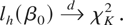
The coverage accuracy of I_hc depends on the asymptotic distribution of the l_h(β₀) statistic. As we shall see subsequently, under suitable regularity conditions, l_h(β₀) has an asymptotic χ_K² distribution, and hence c might be chosen using this result.⁶

Now we comment on the main features of the SEL confidence regions. First, because they are based on the likelihood function, they do not depend on any explicit estimate of Λ₀. This is an advantage over the confidence regions that are based on Wald-type statistics (such as (36), (37), and (39) defined in Section 3.1), which depend on explicit estimates of Λ₀ and might subsequently create problems regarding the quality of the estimates. Second, the shapes of the SEL confidence regions are not restricted a priori to be elliptical or rectangular and are allowed to be determined by the likelihood or, equivalently, by the data.⁷

2.2. Asymptotic Equivalence and Coverage Accuracy

In this section, we derive the asymptotic distribution of the SEL estimator and establish asymptotic equivalence of the SEL and QR estimators. We also discuss asymptotic coverage accuracy of the SEL confidence regions.

Let r ≥ 2 be an integer. We denote F(·|x) to be the cumulative distribution function of U_i conditional on X_i = x and define f (·|x) to be the conditional density of U_i with respect to the Lebesgue measure whenever it exists. We need the following assumptions for our main results.

Assumption 1. {(Y_i,X_i) : i = 1,…,n} are i.i.d. random vectors.

Assumption 2. The parameter vector β₀ is an interior point of the compact parameter space B in

.

Assumption 3. X_i has bounded support, and S₀ and D₀ are nonsingular.

Assumption 4. (a) F(0|x) = q for almost every x. (b) For all u in a neighborhood of 0 and almost every x, f (u|x) exists, is bounded away from zero, and is r times continuously differentiable with respect to u.

Assumption 5.

(c) Let

for some L ≥ 1, where G(u) = ∫_v<u K(v) dv. For any

satisfying ∥θ∥ = 1, there is a partition of [−1,1], −1 = a₀ < a₁ < ··· < a_L+1 = 1 such that

is either strictly positive or strictly negative on (a_l−1,a_l) for l = 1,…,L + 1.

Assumption 6. h satisfies (a) nh^2r → 0 and (b) nh/log n → ∞ as n → ∞.

Assumptions 1–5 are similar to Assumptions 1–5 of Horowitz (1998, p. 1333), which were used to establish asymptotic refinement of the SLAD-estimator-based t and χ² tests through bootstrap. Assumptions 1–5(b) are used to establish the asymptotic normality of

and to justify a Taylor expansion for the EL ratio statistic that in turn is used to calculate the coverage probabilities of our SEL confidence regions. The boundedness assumption for X_i (Assumption 3) is made to simplify the proofs in the Appendix. It can be removed at the cost of more complicated proofs. Also, although the distribution U_i given X_i is assumed to be continuous, the distribution of X_i can be discrete unless it is identically zero with probability 1, which is excluded by Assumption 3. Note that the discrete regressors are important for applications with dummy variables. Assumption 5(c) is used to verify a version of Cramér's condition (Lemma 4 in the Appendix) that is necessary to justify a formal Edgeworth expansion for the distribution of l_h(β₀).

Assumption 6 requires that h goes to zero as n → ∞ at a suitable rate. It is satisfied if h ∝ n^−κ for 1/(2r) < κ < 1, where r ≥ 2. Part (a) of Assumption 6 ensures that the smoothing has an asymptotically negligible effect on the distribution of l_h(β₀). On the other hand, part (b) of Assumption 6 requires that h not be too small. It is needed to ensure a minimum level of smoothness of l_h(β₀) that is necessary to derive Cramér's condition for the Edgeworth analysis. Intuitively this assumption makes sense, because Cramér's condition is mainly intended to ensure distributions of statistics to have an absolutely continuous component, but the latter might be hard to attain for l_h(β₀) if h is chosen too small (for a general interpretation of Cramér's condition, see Hall, 1992, p. 57).

We now derive the asymptotic distribution of the SEL estimator and establish asymptotic equivalence of the SEL and QR estimators.

THEOREM 1. Under Assumptions 1–5(b) and 6(a), we have

where Λ₀ is defined in (15).

The asymptotic covariance matrix Λ₀ can be estimated, e.g., by

which is suggested by Powell (1984, 1986). Under the assumptions of Theorem 1, it is not difficult to show that the estimator is consistent for Λ₀. Another way to estimate Λ₀ is to use a bootstrap estimator as in Buchinsky (1995, 2000), e.g., (38) in Section 3.1. The bootstrap estimator has an advantage in the sense that it does not require a choice of h, but its computation can be more demanding than the kernel-based estimators.⁸

We now discuss coverage properties of the SEL confidence regions. To this end, it is convenient to write the empirical log likelihood ratio statistic l_h(β) (given by (8) and (7)) at β = β₀ in terms of standardized variables. That is, we let

for i = 1,…,n, where t = t(β₀), Z_i = Z_i(β₀), and V_n = EZ_i Z_i′. Then, in terms of the standardized variables λ and W_i, l_h(β₀) can be rewritten as

where λ satisfies

We need to introduce additional notation. We let W_i^j denote the jth component of W_i and define

In particular, α^jk = δ^jk, where δ^jk is the Kronecker delta.⁹

This α-A notation was originally used by DiCiccio, Hall, and Romano (1991). For example, for

, we define α^j = EW^j,α^jj = E(W^j)², α^jjkk = E(W^j)²(W^k)², etc., for 1 ≤ j,k ≤ K.

Under the regularity conditions, we first establish that l_h(β₀) has an asymptotic χ_K² distribution.

THEOREM 2. Suppose Assumptions 1–5(b) and 6(a) hold. Then, we have, as n → ∞,

Remarks.

1. Theorem 2 is a nonparametric version of Wilks' theorem (1938), which has first been proved by Owen (1991) in the standard linear regression models. Chen and Hall (1993, Thm. 3.1) have also established a similar result for the quantiles (with no covariates).

2. From the expansion (A.6) and Lemma 1(a) in the Appendix, we can see that n^1/2EZ_i → 0 if nh^2r → 0 and, if E [X_i f^(r−1)(0|X_i)] ≠ 0, n^1/2EZ_i → 0 implies nh^2r → 0. Therefore, if E [X_i f^(r−1)(0|X_i)] ≠ 0, the bandwidth condition 6(a) is in fact a necessary and sufficient condition for l_h(β₀) to have an asymptotic χ_K² distribution.

If c = c_α is chosen such that

then Theorem 2 implies that the asymptotic coverage of the SEL confidence region I_hc will be α, i.e., P(β₀ ∈ I_hc) = P(l_h(β₀) ≤ c_α) = α + o(1) as n → ∞.

We now discuss the higher order properties of the SEL confidence regions. Using an Edgeworth expansion of the distribution of l_h(β₀), we can show that the asymptotic coverage accuracy of I_hc is in fact of order O(n⁻¹).

THEOREM 3. Define c = c_α by (25). Suppose Assumptions 1–6 hold. If we further assume that sup_n nh^r < ∞, then we have, as n → ∞,

Remarks.

1. The expansion (A.23) in the Appendix implies that the bandwidth condition sup_n nh^r < ∞ is not only sufficient but also necessary for the asymptotic coverage error to be of order O(n⁻¹) if E [X_i f^(r−1)(0|X_i)] ≠ 0. If E [X_i f^(r−1)(0|X_i)] = 0, then the result of Theorem 3 still holds even if nh^r diverges as long as nh^2r → 0 and nh/log n → ∞, i.e., Assumption 6 holds.

2. When nh^r → C (< ∞), the expansion (A.23) and the results (A.20)–(A.22) in the Appendix may be used to derive the “optimal” value of C that minimizes the O(n⁻¹) term on the right-hand side of (26). However, this possibility is not practical of interest because of the availability of the Bartlett correction, which is discussed in the next section.

2.3. Bartlett Correction

In the previous section, the coverage error of the EL confidence region I_hc is of order O(n⁻¹). This error might be partly explained by the fact that the mean of the distribution of l_h(β₀) does not agree with that of the χ_K² distribution, i.e., E [l_h(β₀)] ≠ K. Therefore, one might suspect that this discrepancy might be diminished by rescaling l_h(β₀) so that it has the correct mean. This idea is known as the Bartlett correction in the literature. In this section we show that, provided h is chosen suitably, the Bartlett correction reduces the coverage error to O(n⁻²).

From expansion (A.5), we can show that if nh^r → 0

Here and throughout this paper, we use the convention that terms with repeated superscripts are to be summed over. The result (27) suggests that we might consider a confidence region corrected with the Bartlett factor b:

In practice, b is not observed and has to be estimated. Let

denote any n^1/2-consistent estimator of β₀ such as the SEL estimator

or the usual QR estimator

. Define the estimated Bartlett factor to be

and

is the ith row of

. With some calculation, one can show that

The confidence region corrected with

is now defined to be

Theorem 4, which follows, shows that the coverage error of the SEL confidence region is of order O(n⁻²) if it is Bartlett corrected by either b or

.

On the other hand, from (A.21) and (A.22) in the Appendix, we have

where s_i^−1/2 denotes the ith row of S₀^−1/2. This suggests that one might also consider a confidence region

with the Bartlett factor given by

where

. Note that

is computationally simpler than

because it does not depend on the bandwidth parameter h. However, if

is used instead of b, we will not have the same asymptotic accuracy as

because of the relatively large estimation error of

. This is because we have

and hence, with Bartlett factor

, the coverage error is of order O(n⁻¹h) instead of O(n⁻²).

The Bartlett factor

is derived in the same spirit (i.e., to remove the dependence on h) as β₀ in Chen and Hall (1993, Thm. 4.1). However, it is interesting to note that, in our case,

depends not just on q but also on the covariates {X_i : i ≥ 1}, in the regression framework.

The following theorem formally states the preceding results.

THEOREM 4. Define c = c_α by (25). Suppose Assumptions 1–6 hold. If we further assume that sup_n n³h^2r < ∞, then we have, as n → ∞,

Remarks.

1. The result (A.30) in the Appendix implies that the condition sup_n n³h^2r < ∞ is also necessary for the asymptotic coverage error of

to be of order O(n⁻²) if E [X_i f^(r−1)(0|X_i)] ≠ 0.

2. The Edgeworth expansion for the distribution of l_h(β₀) (i.e., eqn. (A.18) in the Appendix) implies that we have, for any c > 0,

where

is a polynomial of degree 1: i.e.,

, where C₀ = [K2^K/2Γ(K/2)]⁻¹tr(Δ) is a constant. This property of

is essential for our Bartlett correction result, because it enables us to remove the term of order n⁻¹ from the right-hand side of (35) by a simple adjustment for the expected value of l_h(β₀). On the other hand, the Edgeworth expansions of Horowitz (1998, Thm. 4.2) for the t- and Wald statistics and their bootstrap analogues have (odd) polynomials (i.e., q(ν_n,·) on p. 1349 of the latter paper) with nonvanishing terms of degrees 3 and 5. The existence of the latter terms, in general, is the main reason why Bartlett correction is not available for bootstrap (for a general discussion of this phenomenon, see DiCiccio, Hall, and Romano, 1991, Sec. 2.3).

3. Bertail (2003) makes an ingenious use of convex duality and LAN (locally asymptotic normality) properties of the EL ratio to show that empirical likelihoods for Hadamard differentiable functionals are Bartlett correctable in a general setting.

is crucial to verify Cramér's condition (or more specifically to verify the inequality (A.11)). Furthermore, contrary to our result, Bertail (2003) considers only an infeasible Bartlett corrected confidence region and does not suggest any explicit estimator of the Bartlett factor.

3.1. Experimental Design

We consider a linear median regression model

where X_i = (1,X_2i)′, β₀ = (β₀₁,β₀₂)′ is a 2 × 1 parameter vector whose true value is β₀ = (1,1)′, the regressor X_2i is generated from a uniform distribution U [1,5], and error satisfies P[U_i ≤ 0|X_2i] = 0.5. We consider three different distributions for the error U_i: (i) Student t distribution with 3 degrees of freedom rescaled to have variance 2 (DGP1), (ii) U_i = 0.25(1 + X_2i)V_i, where V_i ∼ N(0,1) (DGP2), and (iii) chi-square distribution with 3 degrees of freedom recentered to have median zero (DGP3). In DGP2, U_i is heteroskedastic, and in DGP3 the distribution is skewed. DGP1 and DGP2 are the same as the simulation designs of Horowitz (1998), and DGP3 is considered by Chen and Hall (1993).

We consider confidence regions for the parameter vector β₀. We smooth the EL using a second-order kernel (i.e., r = 2) K(u) = (¾)(1 − u²)1(|u| ≤ 1), which is the so-called Bartlett or Epanečnikov kernel. The SEL confidence regions considered are

, which are defined in (17), (33), and (32), respectively. In the simulation results given subsequently, we denote them by SEL1, SEL2, and SEL3, respectively. The confidence region corrected with the true Bartlett factor b (i.e., I_hc^b defined in (28)) is not considered because it is not of practical interest. To evaluate the effect of smoothing the estimating equations, we also consider unsmoothed EL confidence regions (i.e., the case h = 0), and we denote this by EL.

As another benchmark of our simulation experiments, we consider the confidence regions based on the unsmoothed LAD and SLAD estimators. The former is defined to be

where

is the LAD estimator of β₀, c_α is the α-quantile of the χ₂² distribution, and

is defined by (19) with the kernel function given by the second-order kernel

, which was also used by Horowitz (1998). We also consider a confidence region

where Λ* is a bootstrap estimator of Λ₀. The latter is computed by

where

are the B bootstrap estimates for β₀, for the B samples (each of size n) drawn from the empirical joint distribution of original data {(Y_i,X_i) : i = 1,…,n}. The estimate Λ* is based on the original idea of Efron (1979, 1982) and is also used by Buchinsky (1995) in the QR models.

On the other hand, the confidence region based on the SLAD estimator is given by

Here,

is the SLAD estimator of β₀ that solves

and its variance is estimated by

is the integral of a fourth-order kernel given by

and

. The constant

is computed from the following bootstrap procedure. (i) Generate a bootstrap sample {(Y_i*,X_i*) : i = 1,…,n} by sampling the original data {(Y_i,X_i) : i = 1,…,n} randomly with replacement. (ii) Using the bootstrap sample, compute the SLAD estimate

and its variance estimate

and get

. (iii) Estimate the bootstrap distribution of S_n* by the empirical distribution that is obtained by repeating steps (i) and (ii) many (B) times. (iv) Take

to be the α-quantile of this empirical distribution.

Computing the LAD, SLAD, and SEL confidence regions requires choosing a bandwidth h for each. Existing theories suggest the following rules for choosing h. Hall and Horowitz (1990) show that the bandwidth that minimizes the asymptotic mean squared error of the LAD standard error is of order n^−1/5, so this rule might be useful for the LAD confidence regions. Also, using the duality of confidence region and hypothesis testing and Assumption 6 of Horowitz (1998), the bandwidth that is compatible with the SLAD confidence region based on the fourth-order kernel (40) is of order n^−κ, where

. On the other hand, our Theorems 3 and 4 show that when the kernel order r = 2 the uncorrected and Bartlett corrected SEL confidence regions have coverage errors of order O(n⁻¹) and O(n⁻²) if h is of order smaller than n^−1/2 and n^−3/4, respectively. However, all of the preceding rules are justified in an asymptotic sense, and hence they provide little practical guidance in how to choose h in finite samples. We consider a rule of thumb h = c₀ n^γ in our simulations and take γ ∈ [−1.0,−0.9,….,−0.1]. We take c₀ = 1.0 in our experiments, but, as will be seen, the coverage probabilities of the SEL confidence regions vary little over a wide range of c₀ and γ values.

The number of simulation repetitions used is 40,000 for the LAD, EL, and SEL confidence regions. This yields simulation standard errors of approximately 0.0015 and 0.0010 for the simulated coverage probabilities of nominal 90% and 95% confidence regions, respectively. For the BLAD and SLAD confidence regions, however, the number of repetitions is merely 1,000 because of the very long computing times required for simulations with bootstrapping. In this case, the simulation standard errors are approximately 0.0094 and 0.0068 for nominal 90% and 95% levels, respectively. The number of bootstrap repetitions used is also restricted to B = 100 because of heavy computational cost. We consider eight different sample sizes n ∈ [15,20,…,50].

3.2. Simulation Results

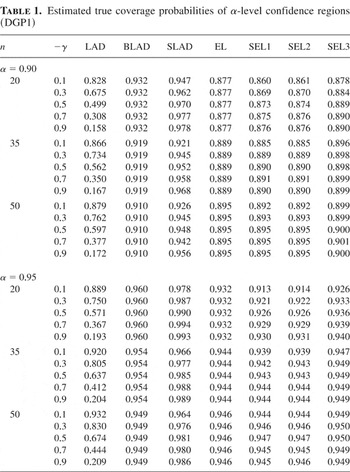
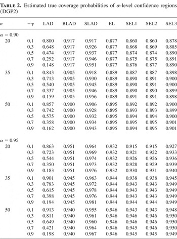
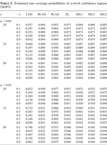
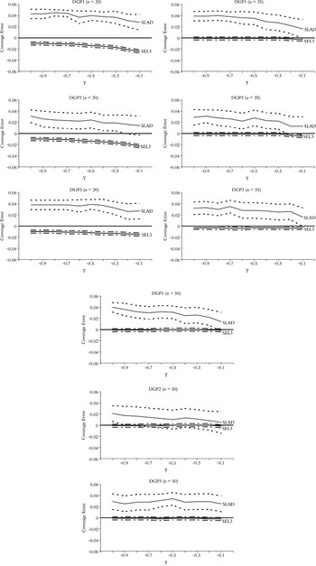
Tables 1, 2, and 3 summarize results for simulated coverage probabilities of confidence regions. Figure 1 shows coverage errors of SLAD and SEL3 (i.e., Bartlett corrected with

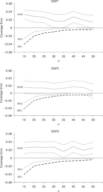
) confidence regions for different values of γ values (which determine bandwidth h). The dotted lines surrounding the solid lines are Bonferroni uniform 95% confidence bands for the coverage errors, which were computed by connecting (1 − 0.05/m) pointwise confidence intervals where m (= 10) is the number of points at which the coverage error was estimated. Figure 2 shows coverage errors of SLAD and SEL1 (i.e., no Bartlett correction) and SEL3 confidence regions for varying sample sizes n. Here we draw the Bonferroni uniform confidence band only for the SLAD case to make the picture less complicated. (The simulation standard errors for SEL1 and SEL3 are virtually negligible because of the large number of repetitions, i.e., 40,000.)

Estimated true coverage probabilities of α-level confidence regions (DGP1)

Estimated true coverage probabilities of α-level confidence regions (DGP2)

Estimated true coverage probabilities of α-level confidence regions (DGP3)

Sensitivity of coverage errors with respect to bandwidth parameters (α = 0.95).

Coverage errors with varying sample sizes (α = 0.95, γ = −0.1(SLAD), −0.9(SEL1, SEL3)).

Our simulation results can be summarized as follows.

1. The coverage probabilities of the LAD confidence regions are relatively poor and very sensitive to the choice of bandwidth. For example, in the DGP1 and n = 35 case, the coverage probabilities of the nominal 95% LAD confidence region are 0.920 and 0.204 for γ = −0.1 and γ = −0.9, respectively. On the other hand, the coverage probabilities of the BLAD confidence regions are relatively very good and stable across different designs.
2. Both the SLAD and SEL confidence regions are robust to the choice of bandwidth. However, Figure 1 shows some evidence that the SEL3 confidence region is less sensitive to bandwidth than the SLAD confidence region, especially for DGP1 and DGP2 and for n ≥ 35.
3. The SEL confidence regions with no Bartlett correction (SEL1) or Bartlett corrected with
   
   (SEL2) perform similarly, though SEL2 is slightly better than SEL1 in almost all cases. This confirms the theory in Theorems 3 and 4(c), which shows that the coverage errors are O(n⁻¹) and O(n⁻¹h) for SEL1 and SEL2, respectively.
4. The SEL confidence regions Bartlett corrected with
   
   (i.e., SEL3) dominate the other confidence regions in most cases. For example, for n = 50, the SEL3 coverage error is virtually zero (up to simulation errors) in almost all cases.
5. The overall performance of the unsmoothed EL confidence regions was similar to that of SEL1 and SEL2. This suggests that, in practice, smoothing of estimating equations is mainly useful to achieve higher order refinements via Bartlett correction.
6. The SLAD confidence regions perform fairly well, especially in small samples (n ≤ 20) and in some cases, outperform SEL1 and SEL2.
7. The effect of increasing the sample size is to reduce coverage errors for almost all confidence regions.
8. Figure 2 shows that, as the sample size increases, SEL3 coverage errors decrease to zero at a faster speed than the SLAD coverage errors. This confirms our theory because the SLAD confidence region has coverage errors of order O(n^−a) for a < 1, whereas the SEL3 confidence region has coverage errors of order O(n⁻²).
9. There is not much difference in relative performance of confidence regions under different DGPs.
10. The results for nominal 90% and 95% confidence regions are similar.
11. The bandwidth that gives the best overall performance for the SEL3 confidence regions is h = n^γ for γ = −0.8. This result is compatible with Theorem 4, which requires −1 < γ < −0.75 for Bartlett correction. Therefore, we recommend using the latter rule of thumb in practical applications, though the results seem to be very robust to the choice of γ.