Introduction

Recent worldwide glacier retreat is one of the clearest consequences of global warming (Reference Lemke and SolomonLemke and others, 2007). Alpine glaciers in particular have experienced a strong retreat since the end of the Little Ice Age (LIA), which has intensified over the last few decades (Reference Paul, Kaab, Maisch, Kellenberger and HaeberliPaul and others, 2004; Reference Bauder, Funk and HussBauder and others, 2007; Reference Huss, Usselmann, Farinotti and BauderHuss and others, 2010). The consequences of this retreat are expected to be very large and dramatic, extending far beyond mere touristic impacts (Reference Elsasser and BurkiElsasser and Burki, 2002). Over the next century, mountain and valley glaciers are expected to make an important contribution to sea-level rise (Reference Kaser, Cogley, Dyurgerov, Meier and OhmuraKaser and others, 2006; Reference Radic = and HockRadic and Hock, 2011; Reference Jacob, Wahr, Pfeffer and SwensonJacob and others, 2012). They are also important water suppliers (Reference Lemke and SolomonLemke and others, 2007), as the annual glacier melting cycle provides water in valleys during the warmest and driest seasons, when it is needed most for consumption, irrigation and cooling. In order to predict the future evolution of glaciers, it is crucial to be able to correctly model and understand their present-day behaviour.

A prerequisite for ice-flow modelling is adequate knowledge of ice geometry over the area of the glacier. Often this is not well known, as there is a lack of direct field measurements, related to difficult and labour-intensive working conditions. However, several techniques exist to deduce the ice thickness distribution without direct field measurements, such as those developed by Reference Li, Li, Zhang and LiLi and others (2011, Reference Li, Ng, Li, Qin and Cheng2012) or the one by Reference Farinotti, Huss, Bauder, Funk and TrufferFarinotti and others (2009), based on glacier mass turnover and principles of ice-flow mechanics. These techniques give good overall results, but are insufficient when applying complex modelling methods at high spatial resolution. In this paper, we reconstruct the thickness field over the Morteratsch glacier complex, Switzerland, based on an extensive field dataset, a high-resolution digital elevation model (DEM) and theoretical relationships such as the plastic flow assumption for central glacier regions.

Several modelling studies have attempted to reconstruct the dynamics of alpine glaciers, extending from simple one-dimensional (1-D) flowline models (Reference OerlemansOerlemans, 1986; Reference Huybrechts, de Nooze, Decleir and OerlemansHuybrechts and others, 1989) through two-dimensional (2-D) models based on the widely used shallow-ice approximation (SIA) (e.g. Reference Le Meur and VincentLe Meur and Vincent, 2003) to complex three-dimensional (3-D) full-Stokes (FS) models (e.g. Reference GudmundssonGudmundsson, 1999; Reference Le Meur, Gagliardini, Zwinger and RuokolainenLe Meur and others, 2004; Reference Jouvet, Huss, Blatter, Picasso and RappazJouvet and others, 2009, Reference Jouvet, Huss, Funk and Blatter2011). In the SIA, horizontal gradients in stress are neglected, which reduces the complexity of the force balance and the boundary conditions. However, this assumption is based on a small aspect ratio between vertical and horizontal characteristic dimension (0th-order approximation), which does not apply to most traditional mountain glaciers as ice thickness is (locally) often of the same order of magnitude as glacier width. Reference Le Meur, Gagliardini, Zwinger and RuokolainenLe Meur and others (2004) have shown that this becomes problematic (i.e. the SIA solution diverges from the FS solution) for mountain glaciers with bedrock slopes above 0.2 and when the maximum ice thickness is of the same order as the glacier span. Another concern of the SIA is that the flow solution is local, ignoring the effect of membrane stresses, yielding unrealistic results in a diagnostic model set-up.

To model the dynamics of alpine glaciers it is therefore more favourable to include longitudinal and transverse stress gradients in the force balance. Here we use a Blatter/Pattyn type of higher-order (HO) 3-D model (Reference BlatterBlatter, 1995; Reference PattynPattyn, 2003; Reference Furst, Rybak, Goelzer, De Smedt, de Groen and HuybrechtsFurst and others, 2011), which is applied to the observed geometry in order to reproduce the flow field of Morteratsch glacier. The model calibration occurs through the tuning of flow and sliding parameters and is based on measured surface velocities (e.g. Reference GudmundssonGudmundsson, 1999). In other work this is often not the case and parameter values are taken from the literature or the calibration is based on indirect field evidence. Examples of the latter are the use of past glacier extents (e.g. Reference Le Meur and VincentLe Meur and Vincent, 2003), which adds a mass-balance uncertainty to the calibration. FS modelling studies have been performed for mountain glaciers elsewhere (e.g. Reference Zwinger and MooreZwinger and others, 2007; Reference Zwinger and MooreZwinger and Moore, 2009), but here also the calibration was not based on direct field measurements.

In this paper we present a new 3-D HO model for the Morteratsch glacier complex. The ice thickness field is reconstructed from an extensive set of radar transects collected from over a decade of field measurements. We then use observations of surface velocity to calibrate constitutive and basal sliding parameters in the model.

Location, Data and Field Measurements

The Morteratsch glacier complex is situated in the southeastern Swiss canton of Graubunden (Fig. 1). It consists of the twin glaciers Vadret da Morteratsch and Vadret Pers. In 2010, the Morteratsch glacier complex had a length of 6.3 km and covered an area of ∼16km2 (Glaciological Reports, 18812011). Vadret Pers flows into Vadret da Morteratsch at a distance of about 1.5 km from the snout. The glacier front is currently at 2050 m elevation, while the highest parts reach 4000 m, culminating at surrounding peaks such as Piz Bernina (PB; 4049 m), Piz Zupo (PZ; 3996 m) and Piz Palu (PP; 3905 m). Like most alpine glaciers, the glacier has undergone a strong retreat since the end of the LIA, with a total retreat of 2.3 km and only 5 years of advance since 1878. Recently this trend has intensified and over the last decade the glacier retreated more than 300 m (Glaciological Reports, 1881-2011).

Fig. 1.

Map of the Morteratsch glacier complex showing glacier elevation together with height contours of the surrounding area at 200m intervals based on a DEM acquired from swisstopo representing the situation in 2001. The map uses the Swiss CH1903 coordinate system. Note that only ice that flows into the glacier complex is considered in the mask and that isolated small glaciers, like Vadret da la Fortezza (situated between Vadret Pers (P) and Vadret da Morteratsch (M)), are not taken into account. The highest surrounding peaks are Piz Bernina (PB; 4049 m), Piz Zupo (PZ; 3996 m) and Piz Palu= (PP; 3905 m). The inset shows the location of the glacier in Switzerland.

A 25 m resolution DEM from 2001 (acquired from the Swiss Federal Office of Topography, swisstopo) is used to obtain the ice mask and surface elevation. This resolution is kept for the ice thickness field reconstruction and for the HO modelling. The fact that the DEM dates from 2001 implies that the thickness field and dynamics reconstruction also represent the state of the glacier in the early 2000s. Therefore, where possible, thickness and surface velocity measurements from the beginning of the last decade (2001– 04) are used. However, except for the lowest parts of the glacier, changes in ice thickness and surface velocity are rather limited over the last 10 years.

Thickness measurements consist of transects and point measurements obtained with a RAMAC monopulse bistatic ground-penetrating radar (GPR) system (Mala Geoscience) in combination with a 5 MHz ice-penetrating point radar system (Reference Narod and ClarkeNarod and Clarke, 1994). The RAMAC GPR data were acquired in common-offset mode with nominal 12.5, 25.0 and 50.0 MHz unshielded antennas for Vadret da Morteratsch and in addition a 100 MHz antenna for Vadret Pers. For the point radar, a monopulse transmitter was used, generating 1600 V pulses across a resistively loaded 10 m antenna. The data acquisition and post-processing, such as rectifications for migration and gain corrections, followed the same methods as described in Reference Eisen, Nixdorf, Keck and WagenbachEisen and others (2003). Regions of the glacier where the ice thickness is known from radar measurements are indicated in Figure 2. The uncertainty in these measurements depends on the equipment (highly frequency-dependent) and the bedrock characteristics, but is usually on the order of 15–20% (Reference Moran, Greenfield, Arcone and DelaneyMoran and others, 2000).

Fig. 2.

Ice thickness derived from radar measurements (coloured points and lines) and locations of the 20 surface velocity points used for model calibration (open circles). The latter correspond to the average position of a network of mass-balance stakes. Grey areas are either ice-free or contain local ice that does not contribute to the flow of the glacier complex.

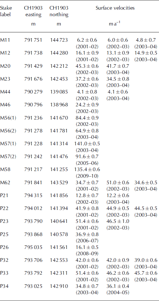
Annual surface velocities are deduced from stake positions, which were measured each year at the end of the ablation season (usually the beginning of October). A Trimble GPS Pathfinder Pro XR was used to determine stake locations. The positions were differentially corrected with nearby Swiss reference stations (located at Samedan or Zimmerwald), which typically reduces the horizontal uncertainty to 0.5-1.0 m. Only measurements from the period 2001-04 were retained for the ice model calibration, except for a few locations where stakes were not available during this reference period. For these, more recent measurements are used, which are considered to be representative of glacier flow in 2001. All the observed surface velocities used for model calibration are summarized in Table 1. Their locations are shown in Figure 2.

Table 1.

Measured annual surface velocities and their respective errors derived from stake positions. The stake locations given in the second and third columns correspond to the average position of the stakes over the respective years. In cases where the velocity of a particular stake is measured over several years, the average is taken and attributed to the midpoint location, except for stakes M56 and M57. These are located at the foot of the Labyrinth icefall in a region of strong spatial velocity gradients and are considered as separate calibration points

Reconstruction of Glacier Thickness and Bedrock Elevation

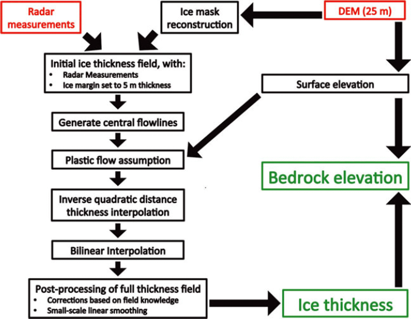
To extend the ice thickness observations (Fig. 2) and obtain a continuous thickness field for the entire glacier, several steps are taken as indicated on the flow chart in Figure 3. First, the 25 m grid is filled with the direct field observations from the radar measurements according to the nearest-neighbour method. These are mostly located in the glacier centre. For gridpoints adjacent to the margins we assume an ice thickness of 5 m. This is realistic for gridpoints situated 12.5 m from the margin (half of the horizontal resolution). Next, central flowlines are generated for all glacier segments. To do this in an automated way, the discrete Laplacian of the distance to the closest margin (di, j) is determined for each gridcell (index i,j) situated more than 125 m from the margin. On a transect, the minimum of the discrete Laplacian corresponds to the point farthest away from the margin, where we assume the ice to be the thickest. The discrete Laplacian (li , j) is calculated using a 2-D finite-difference approximation of the Laplace operator:

(1)

Fig. 3.

Flow chart illustrating the main steps for reconstructing the ice thickness field of the glacier. Red boxes indicate the data sources of input, while green boxes represent the main output.

Cells for which this value is lower than - 5 m are considered to be located on the central flowline. For several locations along this central flowline the ice thicknesses are known from radar measurements. These measurements are used to reconstruct the ice thickness for other locations along the central flowline where the ice thickness was not measured. Under plastic flow theory there is a relationship between ice thickness and surface gradient, given by the yield stress r0. In the SIA this reduces to

(2)

where p is ice density (890kgm–3 for temperate glaciers; Reference Le Meur, Gagliardini, Zwinger and RuokolainenLe Meur and others, 2004), g is the gravitational constant (9.81 m s–2), H is the ice thickness (m) and V h is the surface elevation gradient (known everywhere from the DEM, taken over a horizontal distance of 100 m). The yield stress r0 is first calculated for central regions where radar measurements are available. We obtain a typical value of 150 kPa (144.93 ±27.85 kPa), in good agreement with Reference Cuffey and PatersonCuffey and Paterson (2010). For locations along central flowlines situated more than 200 m from a radar measurement, yield stresses are determined by interpolating the spatially variable yield stresses obtained from radar measurements along the central flowline. These are then inverted to obtain ice thicknesses following Eqn (2).

In a subsequent step, an inverse quadratic distance interpolation of ice thickness is performed between the central flowlines and the margins at regular intervals, except for regions where the ice thickness is known from the field measurements. This ensures a parabolic cross profile as already indicated by the available radio-echo sounding data. Finally, any remaining gaps in the thickness field (because the inverse quadratic distance interpolation was not applied for lines between central regions and margins that cross known measurements) are filled with a bilinear interpolation. From a rock outcropping that occurred in 2006, it is known that ice thickness close to Isla Persa (western side of lower Pers glacier) is overestimated in our reconstruction, which was rectified with a minor manual correction. Finally, a small-scale linear smoothing is applied with a window of 100 m. The bedrock elevation of the Morteratsch glacier complex (Fig. 4b) is then derived by subtracting the reconstructed ice thickness field (Fig. 4a) from the surface DEM. In Figure 4b, we also determined the bedrock elevation below Vadret da la Fortezza using the same principles as described above with a yield stress of 150 kPa. This gave ice thicknesses up to 30 m.

Fig. 4.

(a) Reconstructed ice thickness field. The contours delineate 50 m ice thickness intervals. White areas are either ice-free or have local ice that does not contribute to the flow of the glacier complex. (b) Modelled bedrock elevation obtained by subtracting ice thickness from surface elevation. The thick black line delineates the Morteratsch glacier complex. The thin black lines are bedrock elevation contours at 200 m intervals.

From the DEM, the 2001 area of the Morteratsch glacier complex is 15.8 km2 . The average ice thickness we obtain is 72.2 ± 18.0m and the total glacier volume is 1.14 ± 0.28 km3. The thickest ice is found in the central part of Vadret da Morteratsch at ∼2500 m elevation, where radar measurements indicate an ice thickness up to 350 ± 52.5 m. This is in line with the plastic flow assumption (Eqn (2)), as this is the flattest part of the glacier. The high thickness results in an overdeepening of the glacier bed (Fig. 4b), which is commonly observed in large temperate alpine glaciers (e.g. Glacier d’Argentiere, France: Reference Hantz and LliboutryHantz and Lliboutry, 1983; Aletschgletscher, Switzerland: Reference Hock, Iken and WanglerHock and others, 1999). At the glacier front and for Vadret Pers near the confluence area, there is a strong horizontal gradient in ice thickness resulting in thin ice. The measured low ice thickness for the frontal regions is again in agreement with the plastic flow assumption, as these regions are very steep.

The uncertainty on the reconstructed ice volume and ice thickness distribution is estimated at 25%; 15% of that uncertainty originates from the individual radar measurements while another 20% is attributed to the interpolation procedure. For the latter, uncertainties arise from estimating the yield stress along central flowlines where there are no observations and from any deviation from the assumed parabolic cross section. If it is assumed that both error sources are independent, they can be combined in quadrature.

To compare our methodology with other reconstruction methods, we also applied the method developed by Reference Farinotti, Huss, Bauder, Funk and TrufferFarinotti and others (2009) using the 2-D mass-balance field from Reference Nemec, Huybrechts, Rybak and OerlemansNemec and others (2009). In general this gave comparable results for ice thickness; in both cases the highest ice thickness of Vadret da Morteratsch was found to be ∼ 5 0% larger than that for Vadret Pers. This is due to the similarity between the two methods. Reference Farinotti, Huss, Bauder, Funk and TrufferFarinotti and others (2009) first determine the local ice thickness as the fifth-power root of the mean specific ice volume flux (and other non-local factors). Subsequently these are divided by a factor of sin Vh raised to the power 3/5. This implicitly makes ice thickness inversely proportional to surface slope, as is the case under the plastic flow assumption (see Eqn (2)). Locally, however, the results obtained from Farinotti’s technique differed in some places from our radar measurements. The ice thickness of the lower glacier tongue tends to be overestimated in their method due to the high estimated ice volume flux for these regions.

Larger uncertainties in the geometry reconstruction exist for the higher parts of the glacier, as direct thickness measurements are only available for the saddle area between Piz Bernina and Piz Zupo. Steep slopes and visual observations of ice thickness of several hanging glaciers suggest thin ice of the same magnitude as in our reproduced thickness field. Overall, we have sufficient confidence in the reconstructed ice thickness and bedrock elevation to use it as input to model the glacier flow as detailed further below.

Description of the Ice-Flow Model

We use a finite-difference HO model of Blatter/Pattyn type (Reference BlatterBlatter, 1995; Reference PattynPattyn, 2003; Reference Furst, Rybak, Goelzer, De Smedt, de Groen and HuybrechtsFurst and others, 2011) that solves the 3-D momentum balance according to the LMLa (Multilayer Longitudinal Stresses) approximation (Reference HindmarshHindmarsh, 2004). In contrast to SIA models, this model includes longitudinal and transverse stress gradients. Compared to the FS solution the HO solution assumes cryostatic equilibrium in the vertical, neglecting the vertical resistive stresses, i.e. bridging effects. A related assumption is that horizontal gradients of the vertical velocity are small compared with the vertical gradient of the horizontal velocity, so that the model solves solely for the horizontal velocity components. As the HO solution used here is only accurate to first order, it is not expected to resolve the details of the flow pattern at horizontal resolutions less than a few ice thicknesses.

Owing to a new discretization of the governing force-balance equation that makes extensive use of information on staggered gridpoints (Reference Furst, Rybak, Goelzer, De Smedt, de Groen and HuybrechtsFurst and others, 2011), the model has lower computational costs and is numerically more robust (improved convergence) than older versions of the same LMLa code (Reference PattynPattyn, 2003). Here we use the same horizontal resolution as the DEM (25 m) and consider 21 layers in the vertical. The high horizontal resolution of 25 m is chosen because it allows for a good numerical convergence and because several steps in this paper rely on a nearest-neighbour operation. This is the case for the measured ice thicknesses for deriving the thickness field and for the observed surface velocities used to calibrate the flow parameters. In this way the observations can be located close to their real positions. Nonetheless, the results should not be interpreted at 25 m resolution but rather at a lower horizontal resolution of ∼100-200 m. This is because the 25 m resolution is below the typical ice thickness and the first-order momentum balance on which our model is based does not provide any meaningful information at such a fine resolution. Furthermore, the geometric input is not everywhere representative at a 25 m resolution, as a part of the thickness field is derived through inter- and extrapolation. In addition, a final smoothing of this field was applied at the 100 m scale more in accordance with the approximations underlying the flow model.

Unless stated otherwise, the theoretical and numerical implementations are the same as described in Reference Furst, Rybak, Goelzer, De Smedt, de Groen and HuybrechtsFurst and others (2011). We assume the glacier is temperate, but neglect the pressure-melting effects by assigning a temperature of 0°C everywhere (Reference Cuffey and PatersonCuffey and Paterson, 2010).

As the constitutive equation for ice deformation, Nye’s generalization of Glen’s flow equation is used (Reference GlenGlen, 1955; Reference NyeNye, 1957):

(3)

(4)

where rij are deviatoric stresses and n is the power-law exponent. A0 is the rate factor and the first variable used for model calibration. In this study we take n to be equal to 3, which is its most common value found in the literature (Reference Cuffey and PatersonCuffey and Paterson, 2010). A0 is one of two variables that are tuned to match the observed surface velocities. 77 is the effective viscosity, defined via the second invariant of the strain rate e2 e = 1 t i j t i j . The strain-rate tensor is defined in terms of velocity gradients eij=12(diuj-\-djui). e0 is a negligible offset of 10–30 that makes viscosity finite (Reference PattynPattyn, 2003).

As a lower boundary condition, a Weertman-type sliding law (Reference WeertmanWeertman, 1964) is adopted in which the basal sliding velocity (ub) is proportional to basal drag (Tb , basal shear stress) raised to the third power, a common approach in alpine glacier modelling (e.g. Reference Le Meur and VincentLe Meur and Vincent, 2003; Reference Jouvet, Huss, Funk and BlatterJouvet and others, 2011):

(5)

The basal drag Tb is calculated following the HO approximation and corresponds to the sum of all basal resistive forces (Reference Van der Veen and WhillansVan der Veen and Whillans, 1989):

(6)

in which b is the bedrock elevation. Asl is the sliding parameter and is the second variable used for model calibration. This is incorporated by a Picard iteration on the basal boundary condition. The SIA is used for an initial guess of the basal drag (Tb,SIA), after which the basal drag is updated at each iteration with the basal drag calculated from the HO model at the previous iteration:

(7)

This iterative set-up is similar to the implementation of a Coulomb friction type of basal boundary condition by Reference Bueler and BrownBueler and Brown (2009).

The iterative solver is the same as described by Reference Furst, Rybak, Goelzer, De Smedt, de Groen and HuybrechtsFurst and others (2011). It decomposes the momentum balance into a linear system of equations and a nonlinear update. To reach convergence, the solvers use a relative error for the linear and nonlinear part, which has to fall below 10- 4.

Model Calibration

Calibration using observed surface velocities

By varying the rate factor A0 and the sliding parameter Asl we seek a best fit between the modelled surface velocity field and the observed surface velocities (Table 1). An ensemble of 100 runs were done, each with a different combination of A0 (from 0.6 x 10–16 Pa-3 a- 1 in steps of 0.2 x 10–16 Pa-3 a- 1 to 2.4 x 10–16 Pa-3 a-1) and Asl (from 0 x 10– 1 6m7 N–3 a- 1 in steps of 2 x 10–1 6m7 N–3 a- 1 to 18 x 10–1 6m7 N–3 a-1). For each of these runs the root-mean-square error (RMSE) between the modelled surface velocity (vmod) and the observed surface velocity (vobs; n= 20) is calculated:

(8)

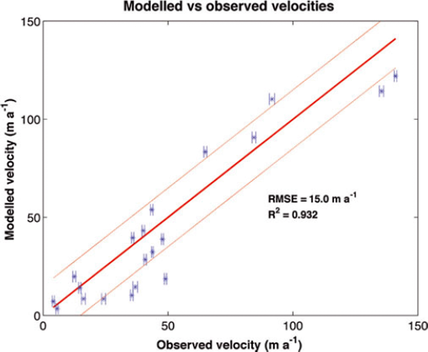
The obtained RMSE for the different runs is summarized in Figure 5. The best agreement between observed and modelled velocities is obtained for the run with A0=1.6x 10–16Pa-3a-1 and As l = 1 2 x 1 0 - 1 6m7 N- 3 a - 1 with an RMSE equal to 15.0 m a- 1 . For this run (Fig. 6), internal deformation accounts on average for 70% of the flow and basal sliding for the remaining 30%. Locally, however, this ratio can vary significantly. Overall, the model is able to reconstruct the observed surface velocities with a large resultant correlation and a high coefficient of determination R2 of 0.93:

Fig. 5.

RMSE between observed and modelled surface velocities for runs with different combinations of A0 and Asl.

Fig. 6.

Modelled versus observed surface velocities (±1<r) for the run with the lowest RMSE (A0 = 1.6 x 10–16Pa–3a–1, Asl =12x 10– 1 6 m7N– 3 a–1). The horizontal bars represent the error on the observed velocity. The thick red diagonal line represents the 1 :1 ratio between observed and modelled velocities. Dashed red lines represent the 1:1 ratio ± RMSE.

(9)

A0= 1.6 x 10–16 Pa-3 a- 1 is of the same order of magnitude as values obtained in other alpine glacier modelling studies. Reference GudmundssonGudmundsson (1999) found a value of 0.75 x 10–16 Pa-3 a-1 for Unteraargletscher, Switzerland, Reference Le Meur and VincentLe Meur and Vincent (2003) 0.63 x 10–16 Pa-3 a- 1 for Glacier de Saint-Sorlin, France, and Reference Iken and TrufferIken and Truffer (1997) 1.6 x 10–16Pa–3a–1 for Findelengletscher, Switzerland. Our value is close to the widely used value of 2.1 x 10–16Pa–3a–1 (Reference PatersonPaterson, 1994). When multiplied with the average glacier thickness of 72.2 m, the sliding factor is Asl = 8.7 x 10–1 4m8N–3 a- 1 (in literature often a division by H occurs in the sliding law), close to the value of 5 x 10–14m8N–3a–1 obtained by Reference Le Meur and VincentLe Meur and Vincent (2003).

Besides the ‘best-fit’ combination, other parameter combinations also give low RMSEs. In fact, a diagonal with minimum RMSE can be identified in Figure 5. This is because A0 and Asl are linearly correlated with, respectively, the internal deformation and sliding. Internal deformation and basal sliding produce a rather similar velocity pattern, as both depend on shear stress raised to the third power. In other words, there is a trade-off between sliding and internal deformation. For instance, a model run with A0 = 1.4x 10–16Pa-3a-1 and As l = 1 8 x 1 0 - 1 6m7 N- 3 a - 1 , in which sliding accounts for almost half of the observed velocities, yields an RMSE of ∼15.5ma–1 . Based on the RMSE only, it is therefore difficult to determine with high confidence the separate contribution of internal deformation and basal sliding for the glacier complex.

For our ‘best-fit’ parameter selection, the largest differences between model and observations occur for four points with rather low observed velocities (25-50 m a-1), with the model underestimating the observations (see Fig. 6). These low velocities, important to understanding the present glacier retreat (see below), contribute comparatively less in the calculation of the total RMSE, as the RMSE is based on absolute differences in velocities. To take this into account, we used a weighted sum as an alternative and calculated a relative RMSE (RRMSE):

(10)

Overall, the pattern in RRMSE is similar to that of the RMSE, but the minimum is slightly shifted to A0 = 2.0 x 10–16 Pa-3 a-1 and A s l = 4 x 10–1 6m7 N–3 a- 1 , corresponding to a larger contribution of internal deformation. Furthermore the contrast along the ‘diagonal of minimal error’ is stronger. The previously mentioned model run with A0 = 1.4 x 10–16 Pa–3 a–1 and Asl =18 x 10–16 m7 N–3 a–1 (about half of the velocity explained by sliding) now has an RRMSE that is ∼35% higher than for the run with the minimum RRMSE (A 0 = 2.0 x 10–16 Pa-3 a- 1 , Asl = 4 x10–1 6 m7 N–3 a-1). Considering both the RMSE and the RRMSE, this suggests that the average contribution of internal deformation is larger than that from basal sliding, but that the exact ratio is difficult to establish from our limited number of direct observations.

Velocity field

The modelled surface velocity field with the lowest RMSE (A0= 1.6 x 10–16Pa-3a-1 and Asl =12 x 10–16m7N–3a–1) is represented in Figure 7, while Figure 8 shows the separate contribution of internal deformation and sliding. The highest surface velocities are found for central upper Vadret da Morteratsch in the icefall (‘the Labyrinth’) near the equilibrium-line altitude (ELA) and reach up to 125 m a-1. In the ablation zone of the glacier the faster parts are mostly linked to large ice thickness, while in the accumulation zone the fast velocities are rather explained by steep surface slopes. For the lowest parts of the glacier, the model is able to reproduce the observed very low surface velocities. In the vicinity of the glacier front, the ice is almost stagnant, indicating that there is little to no mass supply from upstream. Because of this, here the annual frontal thinning is almost equal to the local annual surface mass balance, which is usually close to -8mw.e. a-1 (Reference Nemec, Huybrechts, Rybak and OerlemansNemec and others, 2009). This is crucial for explaining the present-day strong retreat of Vadret da Morteratsch and also generally applies to other alpine glaciers with an extended valley tongue. Modelled surface velocities for the lowest parts of Vadret Pers near the confluence with Vadret da Morteratsch are also very low (3-6 m a-1). The limited mass flux (from up-glacier) enhances the thinning of this region and suggests the imminent separation of the two glaciers. In 2001 the ice thickness was less than 50 m here, which, in combination with an annual surface mass balance of about -5mw.e. a- 1 , indicates that the two glaciers will probably separate in less than 5 years.

Fig. 7.

Modelled surface velocity field for the run with the lowest RMSE (A0 = 1.6 x 10–16 Pa–3a–1, Asl = 12 x 10–16m7N–3a–1). The highest modelled flow speed is 125 ma–1.

Fig. 8.

Modelled velocity due to (a) internal deformation and (b) basal sliding for the run with the lowest RMSE (A0=1.6x10 16Pa 3a 1, Asl = 12 x 10–16m7 N–3a–1). For internal deformation the highest velocity is 95 ma- 1 , while for sliding it is 62 ma–1.

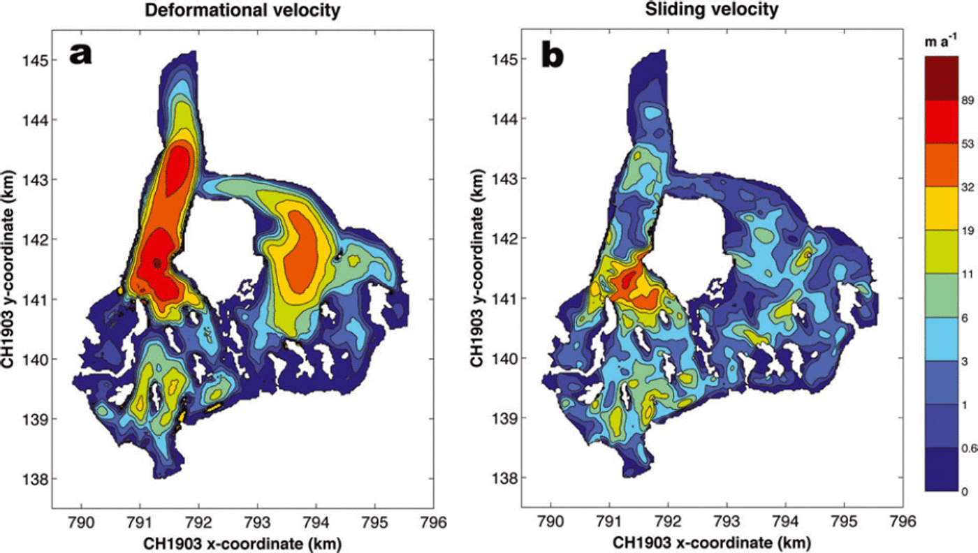
As internal deformation is the main contributor to the flow, a large similarity exists with the modelled surface velocity field. The basal sliding field is more fragmented and reaches high values for the icefall of Vadret da Morteratsch. This is due to the fact that the surface gradient is very high here, combined with moderate ice thickness (Eqn (7)). For the central trunk of Vadret da Morteratsch below the icefall, the fraction of basal sliding is very small due to the low surface slopes.

Conclusion

On the basis of radio-echo sounding data, theoretical concepts and appropriate interpolation techniques, we reconstructed the ice thickness and bedrock elevation of the Morteratsch glacier complex. The thickest ice of up to 350 m was found for the central trunk of Vadret da Morteratsch just below the Labyrinth icefall, while for Vadret Pers the maximum ice thickness is 250 m. The area of highest ice thickness for Vadret da Morteratsch corresponds to an overdeepened bed. Depending on drainage conditions, this may eventually give rise to a proglacial lake if a glacier retreat continues. For this specific glacier, ice thickness reconstruction techniques based on estimates of the mean specific ice volume flux would have provided a generally satisfactory result except in the lower tongue area.

The resulting geometric fields provided an interesting test of the capability of a newly developed HO model code to simulate mountain glacier flow. In such a setting, where the spatial resolution is much higher than for ice-sheet modelling, the robustness and numerical convergence of the ice-dynamic model are crucial. The flow model is able to diagnostically reproduce the observed surface velocities closely (R2 = 0.93). The rate factor (1.6x10–16Pa-3a-1) and sliding parameter (12 x 10–1 6m7 N–3 a–1) obtained from calibrating the model with observed surface velocities are similar to values quoted in the literature. For a best model fit, internal deformation accounts on average for 70% of the glacier flow, and basal sliding for the remaining 30%, even though this ratio varies locally.

The flow model reproduces the almost stagnant front and confluence area between Vadret da Morteratsch and Vadret Pers, which are the most vulnerable parts of the glacier under a warming climate. This suggests a continued severe frontal retreat under present-day climate, and an imminent separation of the two glaciers that make up the Morteratsch glacier complex. Further insight into the rate and timing of this retreat would require a prognostic model in which ice flow is coupled to a surface mass-balance model.