






1. Introduction
The nonstationary (time-dependent) Schrödinger equation, hereafter referred to as the nonstationary Schrödinger equation (NSE), is a fundamental wave equation in non-relativistic quantum mechanics with a wide range of applications. In this paper we study the solutions of NSE associated with a special class of rational potentials that are self-consistent in the sense that the resulting NSE is in fact the focusing nonlinear Schrödinger equation (NLS). Consequently, the NSE solutions describe a class of rational solutions of NLS with non-vanishing boundary conditions, which have been considered in recent times to theoretically describe the phenomenon of extreme or rogue waves. This phenomenon corresponds to spontaneous wave excitations with a high concentration of energy and behave like ‘instantons’, i.e., the waves appear and then disappear very quickly. Such waves have been reported to occur in nature as water waves [Reference Kharif, Pelinovsky and Slunyaev28] as well as in optical fibres [Reference Solli, Ropers, Koonath and Jalali38]. Moreover, they have also been reported in experiments involving water tanks [Reference Chabchoub, Hoffmann and Akhmediev8, Reference Chabchoub, Hoffmann, Onorato, Slunyaev, Sergeeva, Pelinovsky and Akhmediev9], optical fibres [Reference Kibler, Fatome, Finot, Millot, Dias, Genty, Akhmediev and Dudley29, Reference Wabnitz42], plasmas [Reference Bailung, Sharma and Nakamura7, Reference Tsai, Tsai and Lin39] and other physical systems. Analytical modelling of this type of wave phenomena based on rational solutions on a constant background of the NLS equation have been conducted by several authors [Reference Dubard, Gaillard, Klein and Matveev14, Reference Guo, Ling and Liu21, Reference Kedziora, Ankiewicz and Akhmediev27, Reference Ohta and Yang35] using Darboux transformations and Hirota’s bilinear method. More recently, the two-dimensional wave patterns formed by these rational solutions were classified in terms of complex roots of the Yablonskii–Vorobév polynomials and their extensions, which are related to the rational solutions of the Painlevé II hierarchy [Reference Yang and Yang45].
The NSE is also compatible with a linear evolution equation, and they together form a Lax pair whose integrability condition leads to a nonlinear equation satisfied by the NSE potential. This equation is the Kadomtsev–Petviashvili I (KPI) equation, which is a 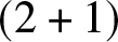 $(2+1)$-dimensional dispersive wave equation describing the propagation of small-amplitude, unidirectional waves with small transverse variation. It was originally proposed by Kadomtsev and Petviashvili [Reference Kadomtsev and Petviashvili25] and has found applications in the study of ion-acoustic [Reference Infeld and Rowlands22, Reference Lonngren32] and shallow water waves [Reference Ablowitz and Segur1, Reference Ablowitz2, Reference Kodama30]. With appropriate time-dependence, the class of NSE potentials considered in this paper constitutes a special family of spatially localized, non-singular and multi-peaked rational solutions of KPI, called the multi-lumps. The multi-lump solutions of KPI were originally found in [Reference Johnson and Thompson24], they were further investigated by several authors including [Reference Ablowitz, Chakravarty, Trubatch and Villarroel3, Reference Chakravarty and Zowada11, Reference Gorshkov, Pelinovsky and Stepanyants20, Reference Pelinovskii and Stepanyants36, Reference Yang and Jianke Yang44] employing direct algebraic techniques. In [Reference Ablowitz and Villarroel4, Reference Villarroel and Ablowitz40] the authors developed an inverse scattering technique to study the NSE with rationally decaying potential and the associated KPI multi-lump solutions. It was shown that in this case NSE admits a discrete spectrum with
 $2$ complex conjugate eigenvalues and the NSE eigenfunction
 $\psi(k)$ is meromorphic in the spectral parameter
 $k \in \mathbb{C}$.
Spectral or algebraic-geometric methods associated with NSE were also employed to construct localized as well as periodic solutions of several nonlinear equations some  $40$ years ago by several authors [Reference Cherednik12, Reference Dubrovin, Malanyuk, Krichever and Makhan’kov16, Reference Krichever31]. In this approach one directly constructs the meromorphic NSE wavefunction
 $\psi(k)$ by imposing a set of restrictions on the spectral data that determines the associated potential satisfying certain self-consistency conditions. The resulting NSE solution
 $\psi$ at special values of the spectral parameter
 $k$ then satisfies a nonlinear equation. A special example of this scheme leading to the construction of rational solutions of the NLS where the NSE potential depends on
 $|\psi(0)|^2$, was studied in [Reference Eleonski, Krichever and Kulagin17]. Subsequently, the results of [Reference Eleonski, Krichever and Kulagin17] were used to construct NLS rogue waves in [Reference Dubard, Gaillard, Klein and Matveev14].
The purpose of this article is to highlight the fact that the NSE wavefunction associated with the NLS rogue waves is also the KPI eigenfunction associated with a special class of KPI multi-lumps. Thus, the NSE provides a bridge between the rational solutions of NLS describing the rogue waves and a special class of multi-lump solutions of KPI with  $n(n+1)/2, \, n \in \mathbb{N}$ peaks. Although this connection was pointed out earlier in [Reference Dubard, Gaillard, Klein and Matveev14, Reference Dubard and Matveev15], these articles essentially follow the work of [Reference Eleonski, Krichever and Kulagin17] where the underlying Baker–Akhiezer function and the meromorphic differentials are unnecessarily complicated. Moreover, it is not obvious from the Wronskian form of the NSE solution whether the obtained rational solutions of NLS and KPI are real and non-singular. The latter assertion requires a more subtle proof that any meromorphic solution to the focusing NLS equation cannot have real poles.
In contrast to the works mentioned in the last paragraph, the present paper adapts a different approach that applies the method of binary Darboux transformation to construct the solution of the NSE, its adjoint and the associated rational NSE potential in the Gramian form. By construction, the resulting NSE eigenfunctions  $\psi(k)$ and its adjoint
 $\phi(k)$ are meromorphic in the spectral parameter. The new result of this paper is to show that if the sums of residues at the poles of the meromorphic functions involving certain products of
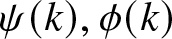 $\psi(k), \phi(k)$ vanish, then
 $\psi(0)$ satisfies the NLS equation. Thus the self-consistency condition satisfied by the NSE potential that leads to the NLS equation can be established in a relatively straightforward fashion. Another important result is that this Gramian formulation guarantees that the constructed potential is real and non-singular.
Significantly, the meromorphic NSE eigenfunctions and its adjoint associated with rational, multi-lump potentials which satisfy the KPI equation, were constructed in [Reference Ablowitz, Chakravarty, Trubatch and Villarroel3]. This particular class of NSE potentials associated with the NLS equation, corresponds to a special family of KPI multi-lumps classified in [Reference Chakravarty and Zowada11, Reference Zowada46] using the theory of integer partitions. In fact, it is shown in this paper that all known rational solutions of NLS describing the hierarchy (higher order) of rogue waves are obtained in this manner. Furthermore, the long-time asymptotics using Schur functions carried out in [Reference Chakravarty and Zowada11] immediately reveal that the local maxima of  $|\psi(0)|^2$ which also correspond to the peak locations of the KPI multi-lumps are given by the complex roots of the Yablonski–Vorobév polynomials and their extensions related to the Painlevé II hierarchy.
The paper is formatted as follows: in Section 2, the NSE wavefunction and the potential are constructed via binary Darboux transformation using a special family of vacuum seed solutions that are expressed in terms of generalized Schur polynomials of odd degree. The generalized Schur polynomials play a fundamental role in the theory of rational, multi-lump solutions of KPI. The resulting NSE wavefunction  $\psi(k)$ and its adjoint
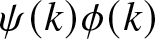
 $\phi(k)$ are meromorphic in the spectral parameter, and more significantly, they satisfy the conditions that the sum of the residues at the poles of the products
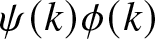 $\psi(k)\phi(k)$ and
 ${\textstyle\frac12(k-b^2/k)\psi(k)\phi(k)}$ vanish. These conditions impose certain constraints between the NSE potential
 $u$ and the square modulus
 $|\psi(0)|^2$ of the NSE wavefunction at
 $k=0$, referred to as the self-consistency condition, and which eventually reduces the NSE to the focusing NLS equation. The rest of Section 2 describes the details of this reduction process. In Section 3, the NLS solution is explicitly constructed as a ratio of determinants that are polynomials in the physical coordinates. Specifically, the denominator is the determinant of a positive-definite, Hermitian matrix. As a result, this construction yields nonsingular, rational solutions of the NLS equation with a constant background. Some examples of such rational solutions are also provided in Section 3, and it is observed that the square modulus of these solutions when viewed as
 $2$-dimensional surfaces, are multi-peaked and arranged in well-defined geometric patterns. In Section 4, the connection between the NLS rational solutions and KPI multi-lumps is established. It is shown that the square modulus of the general NLS solutions exhibits
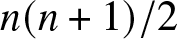 $n(n+1)/2$ local maxima and depends on
 $n$ complex parameters,
 $n \in \mathbb{N}$. The first parameter corresponds to a simple translation of the physical co-ordinates, while if the remaining parameters are identified with real temporal variables, then the underlying NSE potential satisfies a family of evolution equations, the first member of which is the KPI equation. In the remainder of Section 4, asymptotic analysis of these lump solutions for large values of parameter moduli is performed to determine the peak locations and patterns of the multi-lump solutions which describe both the NLS rogue waves as well as
 $2$-reductions of KPI hierarchy. Furthermore, it is shown that asymptotically, the peak patterns are determined by the roots of generalized Yablonskii–Vorobév polynomials associated with special rational solutions of the Painlevé II hierarchy. Section 5 contains some concluding remarks.
2. Construction of NSE solutions
In this section, we construct solutions of NSE using the direct algebraic method of the binary Darboux transformation also known as the Gramian method. We briefly outline the essentials of the method, whose details can be found, for example, in [Reference Matveev and Salle34, Reference Zowada46].
Consider the NSE and its adjoint given by
 \begin{equation}
i\psi_y=\psi_{xx}+u\psi \,, \qquad -i\phi_y=\phi_{xx}+u\phi \,,
\end{equation}
where the subscripts denote partial derivatives and 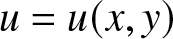 $u=u(x,y)$ is a real potential. Starting from a pair of seed vacuum solutions
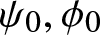 $\psi_0, \phi_0$ of (2.1) with
 $u=0$, one can construct a non-trivial solution of the full NSE (2.1) as follows:
Let  $\{\psi_i, \phi_i\}, i=1,\ldots n$ be a set of linearly independent particular solutions of the vacuum NSE and its adjoint, and let
 \begin{equation}
M_{ij} = \int_x^\infty\psi_i\phi_j\,dx \,, \qquad M_{0j} = \int_x^\infty\psi_0\phi_j\,dx \,, \qquad
M_{j0}= \int_x^\infty\psi_j\phi_0\,dx \,, \,\, 1 \leq i,j, \leq n \,.
\end{equation}
Then the solution of the NSE and its adjoint together with the potential are obtained via the binary Darboux transformation as
 \begin{equation}
\psi = \frac{\det \tilde{M}}{\det M}\,, \qquad \phi = \frac{\det \hat{M}}{\det M}\,, \qquad
u= 2 (\ln\det M)_{xx} \,,
\end{equation}
with the  $n \times n$ matrix
 $M = (M_{ij})$ as defined in (2.2) and the
 $(n+1) \times (n+1)$ matrices
 \begin{equation*}
\tilde{M}= \begin{pmatrix} \psi_0 & M_{01} & \cdots & M_{0n} \\
\psi_1 & && \\
\vdots & & M & \\
\psi_n & && \end{pmatrix} \,, \qquad \quad
\hat{M}= \begin{pmatrix} \phi_0 & M_{10} & \cdots & M_{n0} \\
\phi_1 & && \\
\vdots & & M^T & \\
\phi_n & && \end{pmatrix} \,, \qquad \quad
\end{equation*}
where  $M^T$ denotes the matrix transpose.
It is well known that different choices of the vacuum solutions  $\psi_0, \phi_0$ and
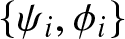 $\{\psi_i, \phi_i\}$ lead to a wide variety of solutions for the NSE with potentials given by
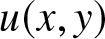 $u(x,y)$ in (2.3). In this note, we are interested in a special class of rational solutions that is illustrated below.
2.1. Special class of rational NSE solutions
Let  $k$ be a complex parameter and
 $\theta(k) := kx+k^2y+\gamma(k)$ where
 $\gamma(k)$ is an arbitrary function, differentiable to all orders, and satisfies
 $\overline{\gamma(\bar{k})} = \gamma(k), \, \gamma(0)=0$. We choose the vacuum solutions of (2.1) as follows
 \begin{equation}
\psi_0(k) := e^{i\theta(k)}\,, \quad \phi_0(k):=e^{-i\theta(k)}\,, \quad \qquad
\psi_j:=\frac{1}{(2j-1)!}D_k^{2j-1}e^{i \theta(k)}\big\vert_{k=k_0}\,, \quad
\phi_j(k_0) := \overline{\psi}_j(k_0) \,,\end{equation}
where ‘bar’ denotes complex conjugate,  $k_0 := ib, \, b \gt 0$ so that the integrals in (2.2) converge, and the differential operator
 $D_k$ is defined by
 \begin{equation}
D_k := \frac{2k^2}{k^2-b^2}\frac{d}{dk} = \frac{d}{dz}\,, \qquad
z(k)=\frac{1}{2}(k+\frac{b^2}{k}) \,.\end{equation}
 $D_k^{2j-1}$ one can re-express
 $\psi_j$ in (2.4a) as
 \begin{equation}
\psi_j = \sum_{l=1}^{2j-1}
\frac{b_{jl}(k_0)}{l!}\partial_k^le^{i\theta}\big\vert_{k=k_0}
= \sum_{l=1}^{2j-1}b_{jl}(k_0)p_l(k_0)e^{i\theta(k_0)} \,, \qquad j=1,\ldots,n \,,
\end{equation}
where the constants 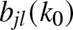 $b_{jl}(k_0)$ will be deduced later, and
 $p_l$ are the generalized Schur polynomials defined by
 \begin{equation*}
\frac{1}{l!}\partial_k^l\exp(i\theta) = p_l(k)\exp(i\theta)\,.
\end{equation*}
These are polynomials in  $x, y$ although they can be expressed in a more natural form as
 $p_l = p_l(\theta_1, \theta_2, \cdots, \theta_l)$ where
 $\theta_j := \textstyle\frac{i}{j!}\partial_k^j\theta$, that is
 \begin{equation}\theta_1=i(x+2ky+\gamma_1),\quad\theta_2=i(y+\gamma_2),\quad\theta_j=i\gamma_j\,,\,\,j \gt 2\,,\quad\gamma_j(k):={\textstyle\frac1{j!}\partial_k^j\gamma(k)\,,\quad1\leq j\leq l\,.}\end{equation}
Thus only  $\theta_1, \theta_2$ depend on
 $x,y$ and the rest are independent complex parameters. In terms of the
 $\theta_j$s the generalized Schur polynomials have the explicit form [Reference Chakravarty and Zowada10]
 \begin{equation}p_l =\sum_\genfrac{}{}{0pt}{}{r_1,r_2,\ldots,r_l \geq 0}{r_1+2r_2+\cdots+lr_l=l}
\prod_{j=1}^{l}
\frac{\theta_j^{r_j}}{r_j!}.
\end{equation}
The first few generalized Schur polynomials are thus given by
 \begin{equation*}p_0=1, \quad p_1=\theta_1, \quad p_2 = \textstyle\frac12\theta_1^2+\theta_2\,, \quad
p_3 = \textstyle\frac{1}{3!}\theta_1^3+\theta_1\theta_2+\theta_3\,, \,\, \ldots \,.\end{equation*}
It follows from (2.7) that the  $p_n$ is a weighted homogeneous polynomial of degree
 $n$ in
 $\theta_j, \, j=1,\ldots,n$, i.e.,
 $p_n(a\theta_1,a^2\theta_2,\cdots,a^n\theta_n)=
a^np_n(\theta_1,\theta_2,\cdots,\theta_n)$, with weight
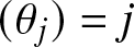 $(\theta_j)=j$. They also satisfy the properties:
 \begin{equation}
\partial^j_{\theta_1}p_n = \partial_{\theta_j} p_n =
\left\{\begin{matrix} p_{n-j}\,, & \quad j\leq n \cr
0\,, & \quad j \gt n \end{matrix} \right.
\end{equation}
 \begin{equation}
p_n(\theta_1+h_1, \theta_2+h_2, \cdots, \theta_n+h_n) =
\sum_{j=0}^n p_j(h_1,h_2,\cdots,h_j) \, p_{n-j}(\theta_1,\theta_2,\cdots,\theta_{n-j})
\end{equation}
Next we proceed to construct the NSE solution  $\psi$ from (2.3) and (2.2) using the particular vacuum solutions in (2.4a). First notice that using (2.5)
 \begin{equation*}M_{0j} = \int_x^\infty \psi \phi_j\,dx =
\sum_{l=1}^{2j-1}b_{jl}(k_0)\int_x^\infty\bar{p}_le^{i(k-\bar{k}_0)x+\cdots}\,dx
= \sum_{l=1}^{2j-1}
\frac{\hat{b}_{jl}}{(k-\bar{k}_0)^{l+1}}\,e^{i(\theta(k)-\bar{\theta}(k_0))}\,,
\end{equation*}
where the last equality is obtained by repeated integration by parts. It shows that  $M_{0j}$ is meromorphic in
 $k$ with a pole of order
 $2j$ at
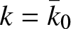 $k=\bar{k}_0$ and the coefficients
 $\hat{b}_{jl}$ depend on
 $\bar{p}_l$ and its
 $x$-derivatives. Hence, these are polynomials in
 $x,y$. Consequently, the NSE solution and its adjoint in this special case are meromorphic in
 $k$ with poles of order
 $2n$ at
 $\bar{k}_0$ and
 $k_0$, respectively, and can be expressed as follows
 \begin{equation}
\psi(k) = \frac{P_n(k)}{(k-\bar{k}_0)^{2n}}e^{i\theta(k)}\,, \quad
P_n(k) =\sum_{j=0}^{2n} a_jk^j\,,
\quad \phi(k) = \overline{\psi(\bar{k})} \,.
\end{equation}
The expression for  $\psi(k)$ above should be evident from the determinant formula in (2.3) by expanding
 $\det \tilde{M}$ using the first row. It should also be clear that the coefficients of the polynomial
 $P_n(k)$, namely,
 $a_j=a_j(x,y; k_0)$ are rational in
 $x,y$. The symmetry
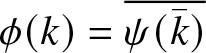 $\phi(k) = \overline{\psi(\bar{k})}$ follows from the choices
 $\phi_0(k) = \overline{\psi_0(\bar{k})}, \phi_i=\bar{\psi}_i$ in (2.4a) which leads to
 $\overline{M_{0i}(\bar{k})} = M_{i0}(k)$ and
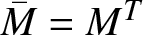 $\bar{M}=M^T$. Furthermore,
 $M$ is a positive definite matrix so that the potential
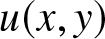 $u(x,y)$ given by (2.3) is real and non-singular.
2.2. Reduction of special NSE to NLS
The special solutions of NSE in (2.9) constructed using the vacuum solutions defined in (2.4a) possess certain unique properties arising from their meromorphicity in the  $k$-space. We describe these properties in this subsection and analyse them to deduce a simple algebraic relation that connects a given NSE solution from this special class to its associated potential
 $u$.
Note that by construction the solutions in (2.9) satisfy the relations
 \begin{equation*} D_k^{2j-1}\psi(k)\big\vert_{k=k_0} = 0 =
D_k^{2j-1}\phi(k)\big\vert_{k=\bar{k}_0} \,, \quad j=1,2,\ldots, n \,, \end{equation*}
which follows from their expressions in (2.3) and by noting that the above operations transform the first row to be identical to the  $j^{\mathrm{th}}$ row in
 $\tilde{M}$ and
 $\hat{M}$, respectively, so that the resulting determinants vanish. Applying (2.4b) to the above expressions and since
 $z(k_0)=z(\bar{k}_0)=0$ with
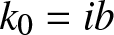 $k_0=ib$, one obtains
 \begin{equation*}\frac{d^{2j-1}}{dz^{2j-1}} \psi(k(z))\big\vert_{z=0} =
\frac{d^{2j-1}}{dz^{2j-1}} \phi(k(z))\big\vert_{z=0} =0 \,, \quad 1 \leq j \leq n \,, \end{equation*}
which implies that near  $z=0$,
 \begin{equation*}\psi(z) = c_0+c_1z^2+\ldots + O(z^{2n})\,, \qquad
\phi(z) = \bar{c}_0+\bar{c}_1z^2+\ldots + O(z^{2n}) \,.\end{equation*}
Next, consider the function  $\zeta(k)=\textstyle\frac12(k-b^2/k)$ which satisfies
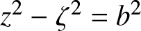 $z^2-\zeta^2 = b^2$ so that
 $\zeta(z) = \sqrt{z^2-b^2}$ and near
 $z=0, \,\,
\zeta(z) = \pm ib \big(1-\textstyle\frac12\textstyle\frac{z^2}{b^2}-\textstyle\frac{1}{8}(\textstyle\frac{z^2}{b^2})^2 - \ldots\big)$. It follows that the functions
 $\psi(z), \phi(z), \zeta(z)$ have no poles at
 $z=0$, hence the residues, namely
 \begin{equation*}\mathop{\mathrm{Res}}\limits_{z=0}\psi(z)\phi(z) = \mathop{\mathrm{Res}}\limits_{z=0}\zeta(z)\psi(z)\phi(z)=0\,. \end{equation*}
Equivalently, one has the conditions that the sum of residues at  $k=k_0, \, \bar{k}_0$
 \begin{equation}
\sum \mathop{\mathrm{Res}}\limits_{k_0,\bar{k}_0}\psi(k)\phi(k) =
\sum \mathop{\mathrm{Res}}\limits_{k_0,\bar{k}_0}\textstyle\frac12(k-b^2/k)\psi(k)\phi(k) =0 \,.
\end{equation}
From (2.9), one has the rational (in  $k$) expression
 \begin{equation}
\psi(k)\phi(k) = \frac{P_n(k)\overline{P_n(\bar{k})}}{(k-k_0)^{2n}(k-\bar{k}_0)^{2n}}
= \frac{k^{4n}+(a_1+\bar{a}_1)k^{4n-1}+(a_1\bar{a}_1+a_2+\bar{a}_2)k^{4n-2}+\cdots+|a_{2n}|^2}
{(k-k_0)^{2n}(k-\bar{k}_0)^{2n}} \,.
\end{equation}
In order to compute the residues at  $k_0, \bar{k}_0$, the following relations are useful
 \begin{align*}
&\sum\mathop{\mathrm{Res}}\limits_{k_0,\bar{k}_0} \frac{k^l}{(k-k_0)^{2n}(k-\bar{k}_0)^{2n}} =0, \,\, l \lt 4n-1\,, \qquad
\sum\mathop{\mathrm{Res}}\limits_{k_0,\bar{k}_0}\frac{k^{4n-1}}{(k-k_0)^{2n}(k-\bar{k}_0)^{2n}} =1\,, \\
& \sum\mathop{\mathrm{Res}}\limits_{k_0,\bar{k}_0}\frac{k^{4n}}{(k-k_0)^{2n}(k-\bar{k}_0)^{2n}} =2n(k_0+\bar{k}_0)\,, \quad
\sum\mathop{\mathrm{Res}}\limits_{k_0,\bar{k}_0}\frac{k^{4n+1}}{(k-k_0)^{2n}(k-\bar{k}_0)^{2n}}
=2n^2(k_0+\bar{k}_0)^2\\ &\qquad\qquad\qquad\qquad\qquad\qquad\qquad\qquad\qquad\qquad\qquad\qquad\qquad\qquad\qquad\qquad +n(k_0^2+\bar{k}_0^2) \,,
\end{align*}
which are easily verified by partial fraction decomposition. These relations in conjunction with (2.11) lead immediately to the following
 \begin{equation*}
\sum\mathop{\mathrm{Res}}\limits_{k_0,\bar{k}_0}\psi(k)\phi(k)=a_1+\bar{a}_1\,, \quad
\sum\mathop{\mathrm{Res}}\limits_{k_0,\bar{k}_0}k\psi(k)\phi(k)= a_1\bar{a}_1+a_2+\bar{a}_2-2nb^2\,, \quad
\sum\mathop{\mathrm{Res}}\limits_{0,k_0,\bar{k}_0}\textstyle\frac{1}{k}\psi(k)\phi(k) =1 \,,
\end{equation*}
where  $k_0=ib$ is also used. Note that
 $k=0$ is a simple pole of
 $\textstyle\frac{1}{k}\psi(k)\phi(k)$ with residue
 $|a_{2n}|^2/b^{4n} = |\psi(0)|^2$. Hence, one needs to subtract this contribution from the third equality above in order to obtain the sum of residues
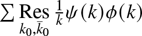 $\sum\mathop{\mathrm{Res}}\limits_{k_0,\bar{k}_0}\textstyle\frac{1}{k}\psi(k)\phi(k)$, i.e., only at
 $k_0, \bar{k}_0$. Collecting all these results together yields
 \begin{equation}
\sum\mathop{\mathrm{Res}}\limits_{k_0,\bar{k}_0}\psi(k)\phi(k) = a_1+\bar{a}_1 \,, \quad
\sum\mathop{\mathrm{Res}}\limits_{k_0,\bar{k}_0}(k-b^2/k)\psi(k)\phi(k) =
|a_1|^2+a_2+\bar{a}_2-(2n+1-|\psi(0)|^2)b^2 \,.
\end{equation}
Moreover, since  $\psi$ in (2.9) is a solution of the NSE,
 $P_n(k)$ satisfies
 \begin{equation*}iP_{ny} = P_{nxx}+2ikP_{nx}+uP_n \,.\end{equation*}
Equating the coefficients of  $k^{2n}$ of this equation, yields
 $u=-2ia_{1x}$. Combining this relation with its complex conjugate and the fact that the potential
 $u$ is real, one obtains
 $(a_1+\bar{a}_1)_x=0$ and
 $iu = (a_1-\bar{a}_1)_x$. The first relation is consistent with the fact that
 $a_1+\bar{a}_1=0$ which follows from the first equations in (2.10) and (2.12). The coefficient of
 $k^{2n-1}$ of the equation for
 $P_n(k)$ gives
 $ia_{1y}=a_{1xx}+2ia_{2x}+ua_1$. Eliminating the
 $y$-derivative by using the complex conjugate of this equation, integrating once with respect to
 $x$, and using
 $a_1+\bar{a}_1=0$, yields the following relation between the potential
 $u$ and the complex coefficients
 $a_1, a_2$
 \begin{equation*} -{\frac{u}{2}} + C(y) = |a_1|^2+a_2+\bar{a}_2 \,,\end{equation*}
where  $C(y)$ is an arbitrary function to be determined later. Substituting the above relation in the second equation of (2.12), the vanishing residue condition from the second equality in (2.10) leads to
 \begin{equation*}b^2\vert\psi(0)\vert^2= \frac{u}{2}+(2n+1)b^2-C(y)\,.\end{equation*}
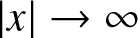
Finally, the boundary conditions:  $u \to 0, \, |\psi(0)| \to 1$ as
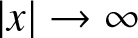 $|x| \to \infty$ (see remark below) imply that
 $C(y) = 2nb^2$ is a constant. Therefore, one obtains the following significant relation connecting
 $\psi(0)$ and the associated potential
 \begin{equation}
u = 2b^{2}(|\psi(0)|^{2}-1) \,.
\end{equation}
Since  $\psi(0)$ satisfy (2.1), one obtains from (2.13)
 \begin{equation}
i\psi(0)_y=\psi(0)_{xx}+2b^2(|\psi(0)|^2-1)\psi(0)\end{equation}
with the boundary conditions for  $\psi(0)$ and
 $u$ mentioned above. The transformation
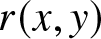
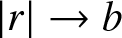
 $r(x,y) = b\psi(0)e^{-2ib^2y}$ leads to the NLS equation
 \begin{equation}
ir_y=r_{xx}+2|r|^2r
\end{equation}
 $r(x,y) \to be^{-2ib^2y}$ as
 $|x| \to \infty$. Equation (2.13) is a self-consistent rational potential associated with the NSE satisfied by the function
 $\psi(0)$ which is also a solution of the NLS equation with non-vanishing boundary condition. Moreover, the obtained solutions for
 $\psi(0)$ are rational in
 $x,y$.
Remark.
(a) An alternate but similar way to arrive at the results above is to consider the residue at
 $k=\infty$ instead of residues at
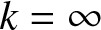
$k_0, \bar{k}_0$. Since
$\psi(k)\phi(k)$ has poles only at
$k=k_0, \bar{k}_0$ whereas
$(k-b^{2}/k)\psi(k)\phi(k)$ has poles at
$k=0, k_0, \bar{k}_0$, it follows from (2.10) that
\begin{equation*}
\sum\mathop{\mathrm{Res}}\limits_{k_0,\bar{k}_0}\psi(k)\phi(k) = \mathop{\mathrm{Res}}\limits_{k=\infty}\psi(k)\phi(k) =0 \,, \qquad
\mathop{\mathrm{Res}}\limits_{k=0}(k-b^2/k)\psi(k)\phi(k) = \mathop{\mathrm{Res}}\limits_{k=\infty}(k-b^2/k)\psi(k)\phi(k) \,.
\end{equation*}
From (2.9) one finds that near
$k=\infty$,
\begin{equation*}
\psi(k) = (1+\textstyle\frac{\psi_1}{k} + \textstyle\frac{\psi_2}{k^2}+ \cdots)e^{i\theta(k)} \,, \qquad
\phi(k) = (1+\textstyle\frac{\bar{\psi}_1}{k} + \textstyle\frac{\bar{\psi}_2}{k^2}+ \cdots)e^{-i\theta(k)}\,.
\end{equation*}Then it follows that
\begin{equation*}
\mathop{\mathrm{Res}}\limits_{k=\infty}\psi(k)\phi(k)=\psi_1+\bar{\psi}_1\,, \qquad
\mathop{\mathrm{Res}}\limits_{k=\infty}(k-b^2/k)\psi(k)\phi(k) = \psi_1\bar{\psi}_1+\psi_2+\bar{\psi}_2-b^2 \,.
\end{equation*}Furthermore since
$\psi(k)$ and
$\phi(k)$ satisfy the NSE and its adjoint, respectively, it follows from the coefficient of
$k^0$ that
$u=-2i\phi_{1x}=2i\bar{\psi}_{1x}$ implying that
$\psi_1+\bar{\psi}_1=0$ (which is consistent with
$\mathop{\mathrm{Res}}\limits_{k=\infty}\psi(k)\phi(k)=0)$ and
$u=-i(\psi_1-\bar{\psi}_1)_x$. The coefficient of
$k^{-1}$ yields
$i\psi_{1y}=\psi_{1xx}+2i\psi_{2x}+u\psi_1$ and its complex conjugate. In the same fashion as previous calculations, one eliminates the
$y$-derivative, integrates once with respect to
$x$ to arrive at
$-u/2+C_1(y) = |\psi_1|^2+\psi_2+\bar{\psi}_2$ where
$C_1(y)$ is arbitrary. Substituting this into the residue conditions above for the function
$(k-b^2/k)\psi(k)\phi(k)$ yields
and as before, from the boundary conditions of
\begin{equation*}b^2|\psi(0)|^2 = \frac{u}{2} +b^2-C_1(y) \,, \end{equation*}
$u$ and
$\psi(0)$ one deduces that
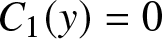
$C_1(y)=0$ which again leads to (2.13).(b) The boundary conditions for the potential and the NSE solution
$\psi(0)$ can be determined as follows. The determinant of the matrix
$M$ constructed from the matrix elements
$M_{ij}$ in (2.2) using the particular vacuum solutions in (2.4a) and (2.5) is of the form
\begin{equation*}\det M = (\text{polynomial in}\, x,y)\exp\big(i
[(k_0-\bar{k}_0)x+(k_0^2-\bar{k}_0^2)y+\gamma(k_0)-\gamma(\bar{k}_0)]\big) \end{equation*}Then the expression
$u(x,y)=2\partial_x^2\ln(\det M)$ implies that the potential
$u(x,y)$ is a rational function of
$x,y$ decaying as
$(x^2+y^2)^{-1}$.The expression for the solution
$\psi(k)$ in (2.9) obtained from (2.3) after using the particular vacuum solutions in (2.4a) can be further analysed to show that
$\psi(k)$ has in fact the form
where
\begin{equation*}\psi(k)=\Big(\frac{k-k_0}{k-\bar{k}_0}\Big)^n\big[1+\sum_{j=1}^n\frac{\mu_j}{(k-k_0)^j}
+\sum_{j=1}^n\frac{\nu_j}{(k-\bar{k}_0)^j}\big]e^{i\theta(k)} \,, \end{equation*}
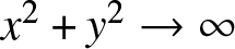
$\mu_j, \nu_j$ are rational in
$x,y$ and decay to
$0$ as
$x^2+y^2 \to \infty$ [Reference Ablowitz, Chakravarty, Trubatch and Villarroel3, Reference Villarroel and Ablowitz40]. Then it is clear that
$|\psi(0)| \to 1$ as
$|x| \to \infty$.
















3. Rational solutions of NLS
The solutions of (2.14b) constructed from the NSE solution  $\psi(0)$ in the previous section are rational, oscillatory solutions which approach a continuous-wave background, i.e.,
 $r(x,y) \to be^{ib^2y}$ as
 $x,y \to \pm\infty$. These NLS solutions have multiple peaks (local maxima) for the function
 $|r(x,y)|$ which exhibit a remarkable set of geometric patterns in the
 $xy$-plane, often termed as rogue wave patterns in the literature. As mentioned earlier in the Introduction, these solutions have been studied extensively both theoretically and numerically; experimental evidence of rogue waves governed by the NLS equation has also been reported in water waves and optical fibres. Although these solutions have been constructed by employing various mathematical techniques by many authors, very few studies have emphasized the fundamental connection between these solutions and NSE. The aim of this paper is to highlight the fact that the rogue wave solutions of the NLS equation are simply special solutions of NSE.
3.1. The Gramian construction
We first obtain an explicit formula for the vacuum solutions given in (2.5) by determining the coefficients 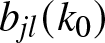 $b_{jl}(k_0)$. Using these, we will derive a Gramian form for the matrix
 $M$ and a similar form for
 $\tilde{M}$ associated with the NSE solution
 $\psi$ and potential
 $u$ in (2.3). We will show that the leading order expansions for
 $\det M$ and
 $\det \tilde{M}$ will provide insights into the structures of the underlying rational solutions of NLS.
From the expression for  $z(k)$ in (2.4b) one can express the branches of inverse function
 $k(z)$ near
 $z=0$ as
 \begin{equation}
k(z) = z \pm ib(1-{\textstyle\frac{z^2}{b^2}})^{1/2} =
z \pm ib \Big(1-{\textstyle\frac{z^2}{2b^2}} -{\textstyle\frac{z^4}{8b^4}} - \cdots \big)
= \sum_{n=0}^\infty k_nz^n \,,\end{equation}
where the coefficients  $k_n$ are given by
 \begin{equation}
k_0 = k(0)=\pm ib, \quad k_1=1, \quad k_3=k_5=\cdots=0,
\quad k_{2j}=(\pm ib)\frac{(-1)^j}{b^{2j}}\genfrac{(}{)}{0pt}{}{\frac{1}{2}}{j} \,.
\end{equation}
 $D_k$ in (2.4b) can be obtained from Faá di Bruno’s formula [Reference Johnson23]
 \begin{align*}
D_k^nf(k)\,\Big\vert_{k=k_0} & = \frac{d^n}{dz^n}f(k(z))\,\Big\vert_{z=0} =
\sum_{l=1}^nB^n_{l}\frac{d^l}{dk^l}f(k)\,\Big\vert_{k=k_0}\,, \qquad\\
B^n_{l} & = n!
\sum_{\begin{matrix}{r_i \geq 0, \,r_1+r_2+\cdots+r_n=l}\\{r_1+2r_2+\cdots +nr_n=n}\end{matrix}}
\frac{k_1^{r_1} \cdots k_n^{r_n}}{r_1!r_2!\cdots r_n!} \,,
\end{align*}
where the coefficients  $k_0, k_1, \ldots, k_n$ are given in (3.1b). The polynomials
 $B^n_{l}(k_1,\cdots,k_n)$ are called Bell polynomials which are associated with set partitions. The expression
 $r_1+2r_2+\cdots+nr_n$ represents the partition of the positive integer
 $n$ into blocks of
 $1$’s,
 $2$’s, etc.,
 $r_i$ denotes the number of blocks of
 $i$, and
 $l$ denotes the number of parts (total number of blocks) in the partition. For example,
 $1+1+1+2+2+3$ is a partition of
 $n=10$ into
 $l=6$ parts with
 $r_1=3, r_2=2, r_3=1, r_j=0, \, j \gt 3$. It is easy to verify from the expression above that
 $B^n_{n}=k_1^n = 1, \,
B^n_1=n!k_n$. Thus from (3.1b),
 $B^n_1=0$ for odd
 $n$ except when
 $n=1$.
The vacuum solutions of NSE given in (2.5) now can be explicitly written as
 \begin{equation}
\psi_j = q_j(x,y,k_0)e^{i\theta(k_0)}\,, \quad
q_j = \sum_{l=1}^{2j-1}b_{jl}(k_0)p_l(x,y,k_0)\,, \qquad
b_{jl} = \frac{l!}{(2j-1)!}B^{2j-1}_l(k_1,\cdots,k_{2j-1}) \,,
\end{equation}
 $j=1,2,\ldots,n$. For example,
 $q_1=p_1$ since
 $b_{11}=B^1_1=1$,
 $q_2=b_{22}p_2+p_3 = 2k_2p_2+p_3$ since
 $B^3_1=0=b_{21},
b_{23}=B^3_3=1$. Similarly,
 $q_3=p_5+4k_2p_4+3k_2^2p_3+2k_4p_2$, and in general for
 $j \gt 1$,
 $q_j$ is a linear combination of the generalized Schur polynomials
 $p_2, \ldots, p_{2j-1}$.
We now proceed to compute the matrix  $M$ in (2.2). Since from (2.4a)
 $\phi_j=\bar{\psi}_j$, the matrix
 $M$ is positive definite. Indeed, for any non-zero vector
 $v \in \mathbb{C}^n$
 \begin{equation*}v^{\dagger}Mv = \sum_{1 \leq i,j \leq n}\bar{v}_iM_{ij}v_j =
\int_x^\infty \left(\sum_{1\leq i,j \leq n}\bar{v}_i\psi_{i}\bar{\psi}_{j}v_j\right)\,dx'
= \int_x^\infty \left(\sum_{i=1}^n|\bar{v}_i\psi_{i}|^2\right)\,dx' \gt 0 \,,
\end{equation*}
Next, substituting  $\psi_j$ from (3.2) and
 $\phi_j=\bar{\psi}_j$ into (2.2) the matrix elements
 $M_{ij}$ can be readily computed by integration by parts, as follows:
 \begin{equation*}M_{ij}= \int_x^\infty\!\!\! \psi_i\bar{\psi}_jdx' =
\int_x^\infty\!\!\! q_i\bar{q}_je^{i(\theta(k_0)-\theta(\bar{k}_0))}dx'
=\frac{e^{i(\theta(k_0)-\theta(\bar{k}_0))}}{2b}H_{ij}\,, \quad \text{with} \end{equation*}
 \begin{equation*} H_{ij}=\sum_{n=0}^{2(i+j-1)}\frac{\partial_x^n(q_i\bar{q}_j)}{(2b)^n}
=\sum_{r=0}^{2j-1}\sum_{s=0}^{2i-1}
\binom{r+s}{s}\frac{\partial_x^r(\bar{q}_j)\partial_x^s(q_i)}{(2b)^{r+s}} \,,\end{equation*}
where  $k_0=ib, \overline{\theta(k)} = \theta(\bar{k})$ and Leibnitz rule of derivatives is used to expand the matrix elements
 $H_{ij}$. Note that the sums in the expressions for
 $H_{ij}$ terminate because
 $q_j$ in (3.2) is a linear combination of the generalized Schur polynomials which satisfy (2.8a) and the fact that
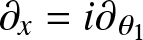 $\partial_x=i\partial_{\theta_1}$ from (2.6). In fact, since the indices
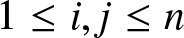 $1 \leq i,j \leq n$ both sums in the last expression for
 $H_{ij}$ above, can be extended to
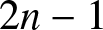 $2n-1$ without affecting the sums as
 $\partial_x^s q_i =0$ if
 $s \gt 2i-1$. Now consider the complex vectors
 \begin{equation*}Q_i = (q_i, \partial_xq_i, \ldots, \partial^{2n-1}_xq_i)^T \in \mathbb{C}^{2n}\,,
\quad i=1,2,\ldots,n \,,\end{equation*}
whose last  $2(n-i)$ components are
 $0$ whenever
 $i \lt n$. Then the matrix elements
 $H_{ij}$ are given by the inner products [Reference Chakravarty and Zowada11]
 \begin{equation*}
H_{ij}=Q_j^\dagger C Q_i \,, \qquad C_{rs} = \frac{1}{(2b)^{r+s}}\binom{r+s}{s}\,,
\quad 0 \leq r,s \leq 2n-1 \,,
\end{equation*}
where  $C$ is a
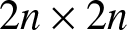 $2n \times 2n$, symmetric matrix. The matrix
 $H$ is Hermitian and has the form
 \begin{equation}
H=Q^\dagger C Q = \begin{pmatrix} \cdots & \bar{Q}_1 & \cdots \\ \cdots & \bar{Q}_2 & \cdots\\
\vdots & \vdots & \vdots \\ \cdots &\bar{Q}_n & \cdots \end{pmatrix} C
\begin{pmatrix} \vdots & \vdots & \cdots & \vdots \\
Q_1 & Q_2 & \cdots & Q_n \\
\vdots & \vdots & \cdots & \vdots \end{pmatrix} \,,
\end{equation}
where  $Q$ is a
 $2n \times n$ matrix of column vectors
 $Q_i, \, 1\leq i\leq n$. The matrix
 $H$ is known as the Gram matrix, and
 $\det H$ is called the Gramian of the vectors
 $Q_1,Q_2,\ldots,Q_n$ which are linearly independent since
 $\det H \neq 0$. In fact
 $H$ is positive definite because
 $M$ is, hence
 $\det H \gt 0$. Consequently, the NSE potential in (2.3) is given by
 \begin{equation}
u = 2 (\ln \det M)_{xx} = 2 (\ln \det H)_{xx} \,,
\end{equation}
as the factor  ${\textstyle\frac{e^{in(\theta-\bar{\theta})}}{(2b)^n}}$ arising in
 $\det M$ is annihilated by
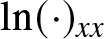 $\ln(\cdot)_{xx}$. Since the generalized Schur polynomial
 $p_j$ is of degree
 $j$ in
 $x,y$, the polynomial
 $q_j$ is of degree
 $2j-1$, hence
 $\det H$ is also a polynomial. Therefore,
 $u(x,y)$ is a nonsingular, rational function of its arguments and decays as
 $(x^2+y^2)^{-1}$. Then it is evident from (2.13) that
 $|\psi(0)|$ and hence, the modulus
 $|r(x,y)|=b|\psi(0)|$ of the NLS solution in (2.14b) is also rational and non-singular.
Next we will derive an expression for the NSE solution  $\psi(k=0)$ from the first of the formulas in (2.3) after using (2.2) to compute the elements
 $M_{0j}$ of the matrix
 $\tilde{M}$. Substituting
 $\psi_0$ from (2.4a) and
 $\phi_j=\bar{\psi}_j$ from (3.2) in (2.2), and applying integration by parts as before
 \begin{equation*} M_{0j}(k)= \int_x^\infty\!\!\! \psi_0(k)\bar{\psi}_jdx' =
\int_x^\infty\!\!\! \bar{q}_je^{i(\theta(k)-\theta(\bar{k}_0))}dx'
=\frac{e^{i(\theta(k)-\theta(\bar{k}_0))}}{2b}H_{0j}(k)\,, \quad \text{with} \end{equation*}
 \begin{equation*} H_{0j}(k)=\frac{2ib}{k-\bar{k}_0}
\sum_{n=0}^{2j-1}\frac{i^n\partial_x^n\bar{q}_j}{(k-\bar{k}_0)^n} \,,
\quad \text{and} \quad H_{0j}(0)=
2\sum_{n=0}^{2j-1}\frac{\partial_x^n\bar{q}_j}{b^n} \end{equation*}
after using  $k_0 = ib$. The matrix
 $\tilde{M}$ is a
 $(n+1) \times (n+1)$ matrix bordered by the elements
 $M_{0j}$ in its first row and
 $\psi_0, \psi_i$ in its first column. Applying the expansion formula of bordered determinants, yields
 \begin{equation*}
\det (\tilde{M}_{ij})(k=0) = \det\Big(M_{ij}-\psi_iM_{0j}(0)\Big) =
\det\tilde{H} \,\frac{e^{in(\theta(k_0)-\theta(\bar{k}_0))}}{(2b)^n}\,, \quad
\tilde{H}_{ij} = H_{ij}-q_iH_{0j}(0) \,.
\end{equation*}
Furthermore, as in (3.3), the matrix  $\tilde{H}$ can also be expressed as
 \begin{equation*}
\tilde{H}=Q^\dagger \tilde{C} Q\,, \quad \tilde{C} = C-D\,, \qquad
D_{rs} = 2b^{-r}\delta_{0s} \,, \quad 0 \leq r,s \leq 2n-1 \,,
\end{equation*}
i.e., the only non-zero elements of  $D$ are
 $2b^{-r}$ in the first column, and
 $C$ is given above (3.3). Then the NSE solution
 $\psi(0)$ of (2.14a) is obtained as a ratio of two Gram determinants, namely
 \begin{equation}
\psi(0) = \frac{\det \tilde{M}(0)}{\det M} =
\frac{\det \tilde{H}}{\det H} =
\frac{\det (Q^{\dagger} \tilde{C} Q)}{\det (Q^{\dagger} C Q)} \,.
\end{equation}
Thus  $\psi(0)$ is a nonsingular, rational function in
 $x,y$ since it is the ratio of polynomials of the same degree and
 $\det H \gt 0$. Moreover, by expanding the leading terms of the determinants in (3.5) one can verify that
 $|\psi(0)| \to 1$ as
 $\sqrt{x^2+y^2} \to \infty$ as mentioned in Remark (b) of Section 2. We will discuss the structure of
 $|\psi(0)|$ and
 $u$ given by (2.13) later, but first we provide some examples of the rational solutions below.
3.2. Examples of rational solutions
The solutions  $\psi(0)$ can be constructed explicitly by expanding the determinants in the numerator and denominator of the last equality in (3.5) by applying Binet–Cauchy formula. When
 $n=1$, the vacuum solution from (3.2)
 $\psi_1 = q_1e^{i \theta(k_0)}=p_1e^{i \theta(k_0)}$ where
 $p_1$ is the generalized Schur polynomial of degree
 $1$. In this case, the matrix
 $Q$ has a single column and
 $C, \tilde{C}$ are
 $2 \times 2$ matrices defined above (3.3) and (3.5), respectively. These are given by
 \begin{equation*} Q= \begin{pmatrix} p_1 \\ \partial_xp_1 \end{pmatrix} \,, \quad
C = \begin{pmatrix} 1 & \frac{1}{2b} \\ \textstyle\frac{1}{2b} & \textstyle\frac{1}{2b^2} \end{pmatrix} \,,
\qquad \tilde{C} = \begin{pmatrix} -1 & \frac{1}{2b} \\ -\textstyle\frac{3}{2b} & \textstyle\frac{1}{2b^2}
\end{pmatrix} \,. \end{equation*}
The matrices 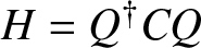 $H=Q^{\dagger}CQ$ and
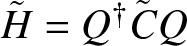 $\tilde{H} = Q^{\dagger}\tilde{C}Q$ are both
 $1 \times 1$, so that
 \begin{equation*} \det H = |p_1|^2-\textstyle\frac{i}{2b}(p_1-\bar{p}_1) + \textstyle\frac{1}{2b^2} \,, \quad
\det\tilde{H} = -\det H + \textstyle\frac{i}{b}(p_1+\bar{p}_1) + \textstyle\frac{1}{b^2} \,, \end{equation*}
where  $p_1 = \theta_1 = i(x+2k_0y+\gamma_1)$ from (2.6) and
 $\partial_x p_1=i\partial_{\theta_1} p_1 = p_0 =1$ from (2.8a). Introducing the coordinates
 $r=x, \, s=2by$ and using
 $k_0=ib$, we can express
 $\theta_1 = i(r+is+\gamma_1)$. Then the corresponding NLS solution is given by
 \begin{equation}
\psi(0) = - 1+\frac{-2i(s-s_0)+\textstyle\frac{1}{b^2}}{(r-r_0)^2+(s-s_0)^2+\textstyle\frac{1}{4b^2}} \,,
\end{equation}
with parameters  $r_0= -\operatorname{\rm Re}\nolimits(\gamma_1), \, s_0=-\operatorname{\rm Im}\nolimits (\gamma_1)$ and
 $b$. Switching
 $\psi(0) \to -\psi(0)$ which does not change (2.14a), one recovers the well-known Peregrine solution [Reference Peregrine37]. Then the corresponding NSE potential is
 \begin{equation*} u = 4\,\frac{-(r-r_0)^2+(s-s_0)^2+\textstyle\frac{1}{4b^2}}
{\big[(r-r_0)^2+(s-s_0)^2+\textstyle\frac{1}{4b^2}\big]^2} \,, \end{equation*}
which can be calculated from (2.13) or directly from (2.3) as  $u=2(\log \det H)_{xx}$.
The solutions  $|\psi(0)|$ and
 $u$ are illustrated in Figure 1, which shows a single peak of height
 $3$ for
 $|\psi(0)|$ and
 $16b^2$ for
 $u$, both at
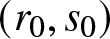 $(r_0,s_0)$. Moreover, the vertical sections (at
 $s=s_0$) indicate that
 $|\psi(0)|$ and
 $u$ have two local minima of depth
 $0$ and
 $-2b^2$, respectively, symmetrically located from the peak at
 $(r_0 \pm \textstyle\frac{\sqrt{3}}{2b})$. Notice also that
 $\psi(0)| \to 1$ while
 $u \to 0$ for large
 $|r|, |s|$.
 $|\psi(0)|$ for the Peregrine solution and the corresponding NSE potential
 $u$. Parameters:
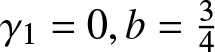 $\gamma_1=0, b=\textstyle\frac34$. Right panels: Vertical cross-section (
 $s=0$) showing the maximum and two minima.

Figure 1 Long description
A showing a 3D surface plot labeled, absolute value of psi 0. The horizontal axes are labeled, s and r, each ranging from minus 5 to 5. The vertical axis has tick labels 0, 1, 2, 3. The surface has one tall central peak and two lower depressions on opposite sides of the peak. B showing a line graph labeled, absolute value of psi 0. The horizontal axis is labeled, r, with tick labels minus 4, minus 2, 0, 2, 4. The vertical axis is labeled, absolute value of psi 0, with tick labels 0, 1, 2, 3. The curve rises to a single peak near r equals 0 at about 3 and has two symmetric minima near r equals minus 2 and r equals 1 at about 0. C showing a 3D surface plot labeled, u. The horizontal axes are labeled, s and r, each ranging from minus 5 to 5. The vertical axis has tick labels minus 5, 0, 5. The surface has one tall central peak and two lower depressions on opposite sides of the peak. D showing a line graph labeled, u. The horizontal axis is labeled, r, with tick labels minus 4, minus 2, 0, 2, 4. The vertical axis is labeled, u, with tick labels 0, 5, 10, 15. The curve rises to a single peak near r equals 0 at about 9 and dips below 0 on both sides near r equals minus 2 and r equals 1.
The higher ( $n \gt 1$) order rational solutions of NLS can be generated in a similar way. For example, one starts with 2 vacuum solutions of NSE
 $\psi_1, \psi_2$ when
 $n=2$, and
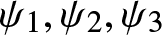 $\psi_1, \psi_2, \psi_3$ for
 $n=3$. From (3.2), these are given as
 $\psi_i=q_ie^{i\theta(k_0)}, \, i=1,2,3$ where
 \begin{equation*} q_1=p_1\,, \quad q_2 = p_3-\textstyle\frac{i}{b} p_2\,, \quad
q_3= p_5 -\textstyle\frac{2i}{b} p_4 - \textstyle\frac{3}{4b^2} p_3 - \textstyle\frac{i}{4b^3}p_2 \,,
\end{equation*}
and  $p_j$s are the generalized Schur polynomials given by (2.7). Then one constructs the
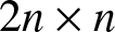 $2n \times n$ matrix
 $Q$ and the
 $2n \times 2n$ matrices
 $C$ and
 $\tilde{C}$ as described in Section 3.1, and finally applies Binet–Cauchy formula to compute
 $\det H$ and
 $\det \tilde{H}$ to construct
 $\psi(0)$ in (3.5). The corresponding expressions are too lengthy even for
 $n=2,3$, hence they are omitted here. Instead, these solutions are illustrated in Figures 2 and 3. They show that both
 $|\psi(0)|$ and
 $u$ are localized around multiple peaks whose numbers are 3 and 6 for
 $n=2$ and
 $n=3$, respectively. The peaks can be well-separated by increasing the magnitude of the parameter
 $\gamma_3$. Moreover, in the neighbourhood of each local maximum, the solution is effectively a Peregrine solution with the same peak height and with two local minima symmetrically placed around the peak. We will discuss the structure of these rational NLS solutions for arbitrary values of
 $n$ including the number and location of the peaks as well as peak patterns in the next section where we connect these solutions to the multi-lump solutions of the KPI equation.
 $3$-lump solutions of the NLS equation. Parameters:
 $\gamma_1=\gamma_2=0, \gamma_3 = 100, b=\textstyle\frac12$. Left panel:
 $|\psi(0)|$, right panel:
 $u$.

 $6$-lump solutions of the NLS equation. Parameters:
 $\gamma_1=\gamma_2=0, \gamma_3 = 80, \gamma_5=0, b=\textstyle\frac12$. Left panel:
 $|\psi(0)|$, right panel:
 $u$.

4. Multi-lumps of NLS and KPI
The examples in Section 3 demonstrate that the  $n$-lump solutions for
 $n=2$ and
 $n=3$ exhibit, respectively,
 $3$ and
 $6$ distinct peaks whose heights approach the
 $1$-lump peak height asymptotically when the magnitude of the parameter
 $\gamma_3$ is large. In this section, we will discuss the general features of the
 $n$-lump solutions, and show that they have
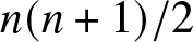 $n(n+1)/2$ distinct peaks and are parametrized by
 $n$ complex parameters. The observation that is key to establish these and other properties of the
 $n$-lumps is the fact that the NSE solution
 $\psi(0)$ and the potential
 $u$ satisfying the NLS equation (2.14a) are also associated with the KPI hierarchy. In particular, the NSE potential
 $u$ in (3.4) satisfies the KPI equation
 \begin{equation}
(4u_t+6uu_x+u_{xxx})_x=3u_{yy}.
\end{equation}
when the evolution variable  $t$ is identified with the parameter
 $\gamma_3$. Indeed, it is known from Sato theory that the NSE (2.1) is a member of an infinite family of compatible linear evolution equations in
 $\psi = \psi(t_1,t_2,\ldots,)$ with respect to the multi-time variables
 $t_1=x, t_2 = y, t_3, \ldots$. The associated compatibility conditions of this infinite family of linear equations lead to the KPI hierarchy. We adapt the framework of the KP theory below in the binary Darboux construction of the rational solutions of NSE in Section 2.
4.1. KPI multi-lumps
The binary Darboux transformation of Section 2 can be extended to construct the solutions of the KPI hierarchy by considering the linear system
 \begin{equation*}i^{n-1}\partial_{t_n}f = \partial^n_xf\,, \quad n \in \mathbb{N} \end{equation*}
which includes the vacuum NSE when  $n=2$ and
 $t_2=y$. A particular solution to this system is given by
 $\psi_0(k) = e^{i\theta(k)}$ as in (2.4a) with
 \begin{equation*} \theta(k) = kx+k^2y+\gamma(k)\,, \quad \gamma(k)=\sum_{n \gt 2}k^nt_n \,. \end{equation*}
Furthermore, the functions 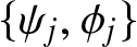 $\{\psi_j, \phi_j\}$ defined in (2.4a) (as well as in subsequent equations (2.5) and (3.2)) in terms of the generalized Schur polynomials
 $p_n(\theta_1, \ldots, \theta_n)$, also solve the above linear system and its adjoint. The generalized Schur polynomial variables
 $\theta_j$ given by (2.6) now depend on the multi-time variables through the parameters
 $\gamma_j=\gamma_j(t_3, t_4, \ldots)$. Then the solution
 $\psi$ and the potential
 $u$ given by (2.2) and (2.3) constitute the multi-time KPI hierarchy. In particular, the KPI equation (4.1) is the first non-trivial member of the hierarchy with
 $t_3=t \in \mathbb{R}$. Consequently, the Gramian construction in Section 3 leads to a special class of rational solutions of KPI given by (3.4) which is also related to the NLS equation (2.14a) via (2.13).
It is useful to examine the structure of the solution  $u$ in (3.4) in some details in order to gain insight into the structure of the rational solutions of NLS. The real symmetric matrix
 $C$ in (3.3) admits a Cholesky decomposition
 $C=U^{\dagger}DU$ where
 $U$ is a real, upper-triangular matrix with 1’s along its main diagonal and
 $D$ is a diagonal matrix, i.e.,
 \begin{equation*}
D = \mathrm{diag}((2b)^{-2r})\,, \quad
U_{rs} = \left\{\begin{matrix}\frac{1}{(2b)^{s-r}}\binom{s}{r}\,,
& \quad r\leq s\cr 0\,, & \quad r \gt s \end{matrix} \right. \,.
\qquad r,s=0,1,\ldots, 2n-1 \,.
\end{equation*}
Then in (3.3), 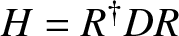 $H=R^{\dagger}DR$ with
 $R=UQ$. Consequently,
 $\det H$ can be expressed as a sum of squares after using the Binet–Cauchy formula
 \begin{equation}
\det H = \sum_{0 \leq l_1 \lt \cdots \lt l_n \leq 2n-1}
\frac{|R(l_1 \cdots l_n)|^2}{(2b)^{2(l_1+\cdots+l_n)}}\,,
\qquad R(l_1 \cdots l_n)=\sum_{0 \leq r_1 \lt \cdots \lt r_n \leq 2n-1}
U\binom{l_1 \cdots l_n}{r_1 \cdots r_n}Q(r_1 \cdots r_n) \,,\end{equation}
where  $R(l_1 \cdots l_n)$ is the principal minor of the
 $2n \times n$ matrix
 $R$ whose columns are
 $UQ_i, \, 1 \leq i \leq n$ and rows are indexed by
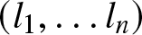 $(l_1,\dots l_n)$. The
 $n \times n$ minor
 $U\tbinom{l_1 \cdots l_n}{r_1 \cdots r_n}$ of
 $U$ is obtained from the submatrix whose rows and columns are indexed by
 $(l_1,\dots l_n)$ and
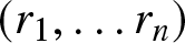 $(r_1,\dots r_n)$, respectively, and
 $Q(r_1 \cdots r_n)$ is the principal minor of
 $Q$ with rows indexed by
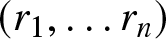 $(r_1,\dots r_n)$. Since
 $U$ is upper triangular with
 $1$’s along its diagonal, it follows that the principal minors
 $U\tbinom{l_1 \cdots l_n}{l_1 \cdots l_n}=1$ and
 $U\tbinom{l_1 \cdots l_n}{r_1 \cdots r_n} \neq 0$ if and only if
 $l_j \leq r_j$ for each
 $j=1,\ldots,n$. Consequently, the determinant in (4.2a) can be re-expressed as
 \begin{equation}
\det H = \frac{|R(\textbf{0})|^2}{(2b)^{n(n-1)}} + \sum_{\textbf{r} \gt \textbf{0}}
\frac{|R(\textbf{r})|^2}{(2b)^{|2\textbf{r}|}} \,,
\quad \qquad
R(\textbf{0}) = Q(\textbf{0}) + \sum_{\textbf{r} \gt \textbf{0}}
U\binom{\textbf{0}}{\textbf{r}}Q(\textbf{r})\end{equation}
 $\textbf{r} := (r_1 \cdots r_n), \, 0 \leq r_1 \lt r_2 \lt \cdots \lt r_n \leq 2n-1$ denote lexicographically ordered multi-index sets whose earliest member is
 $\textbf{0} := (01 \cdots n-1)$, and
 $|\textbf{r}| := r_1+\cdots + r_n$. In terms of the polynomial
 $q_j$ in (3.2), these maximal minors can be expressed as
 \begin{equation}Q(\textbf{r})=\begin{vmatrix}q_1^{(r_1)}&q_2^{(r_1)}&\cdots&q_n^{(r_1)}\\q_1^{(r_2)}&q_2^{(r_2)}&\cdots&q_n^{(r_2)}\\\vdots&\vdots&\vdots&\vdots\\q_1^{(r_n)}&q_2^{(r_n)}&\cdots&q_n^{(r_n)}\end{vmatrix}\,,\qquad Q(\textbf{0})=\begin{vmatrix}q_1&q_2&\cdots&q_n\\q_1^{(1)}&q_2^{(1)}&\cdots&q_n^{(1)}\\\vdots&\vdots&\vdots&\vdots\\q_1^{(n-1)}&q_2^{(n-1)}&\cdots&q_n^{(n-1)}\end{vmatrix}\,,\end{equation}
where the superscripts denote derivative with respect to  $x$, and
 $q_j^{(r)}=0, \, r \gt 2j-1$ (cf. Section 3.1). In particular, note that
 $Q(\textbf{0}) = \operatorname{\rm Wr}\nolimits(q_1,q_2,\ldots,q_n)$ is a Wronskian.
Recall from Section 2 that the generalized Schur polynomials  $p_l$ are weighted homogeneous polynomials of degree
 $l$ in
 $\theta_1, \theta_2, \ldots, \theta_l$ with weight
 $(\theta_j)=j, \,
1 \leq j \leq l$. Moreover, from (2.6),
 $\theta_1=i(r+is+\gamma_1)$ in terms of the physical coordinates
 $x=r, s=2by$ (note that for KPI solutions,
 $r=x-3b^2t$ where
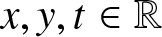 $x,y,t \in \mathbb{R}$ are the physical variables). Then the determinant
 $Q(\textbf{r})$ is a weighted homogeneous polynomial in
 $\theta_1, \theta_2, \ldots, \theta_{2n-1}$ of degree
 $(1+3+\cdots+2n-1)-|\textbf{r}|$. Particularly when
 $\textbf{r} = \textbf{0}$, the degree of the leading principal minor
 $Q(\textbf{0})$ is the highest in the coordinates
 $r,s$, and is given by
 \begin{equation*}(1+3+\cdots+2n-1)-\textstyle\frac{n(n-1)}{2} =n(n+1)/2 \,. \end{equation*}
Thus,  $\det H$ in (4.2) is a positive definite polynomial in
 $r$ and
 $s$ of degree
 $n(n+1)$ and with
 $2n-1$ complex parameters
 $\gamma_j, \, 1 \leq j \leq 2n-1$ which appear in the arguments
 $\theta_j, \, j=1,\ldots, 2n-1$ of the generalized Schur polynomials. However, it turns out that the minors
 $Q(\textbf{r})$ in (4.3) depend on only
 $n$ independent combinations of these parameters. The proof of this fact is somewhat technical, only the basic ideas are outlined below.
First, note that for each  $j=1,2,\ldots,n$ the polynomial
 $q_j$ in (3.2) can be transformed to a single generalized Schur polynomial with shifted arguments by using the property (2.8b), i.e.,
 \begin{equation*}q_j = \sum_{l=1}^{2j-1}b_{jl}\,p_l(\theta_1, \theta_2, \cdots, \theta_l)
= p_{2j-1}(\hat{\theta}_1, \hat{\theta}_2, \cdots, \hat{\theta}_{2j-1}) \,,
\quad \hat{\theta}_k = \theta_k+h^j_k\,, \quad 1 \leq k \leq 2j-1 \end{equation*}
The shifts  $h^j_k$ can be suitably chosen such that the coefficients
 $b_{jl} = p_{2j-1-l}(h^j_1,h^j_2, \ldots, h^j_{2j-1-l})$. Note that the shifts do depend on the index
 $j$ of the polynomial
 $q_j$, that is,
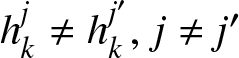 $h^j_k \neq h^{j'}_k, \, j \neq j'$. Then each column of the matrix
 $Q$ is expressed as
 \begin{equation*}Q_j= (q_j, \partial_xq_j, \ldots, \partial^{2n-1}_xq_j)^T
= (p_{2j-1}(\hat{\theta}), ip_{2j-2}(\hat{\theta}), \ldots, i^rp_{2j-r-1}(\hat{\theta}), \ldots,
i^{2n-1}p_{2j-2n}(\hat{\theta}))^T\,, \end{equation*}
where  $p_l(\hat{\theta}) := p_l(\hat{\theta}_1, \ldots, \hat{\theta}_l)$. Next, decompose the even-indexed argument
 $\hat{\theta}_{2k} = \hat{\theta}^0_{2k}+\gamma_{2k}, \,
1 \leq k \leq j-1$ of each generalized Schur polynomial
 $p_{2j-1}$ in the first row of the matrix
 $Q$ and expand using (2.8b) to yield
 \begin{equation*}p_{2j-1}(\hat{\theta}) = \sum_{r=0}^{j-1}p_{2r}(0,\gamma_2,0,\gamma_4, \ldots, 0, \gamma_{2r})
p_{2j-1-2r}(\hat{\theta}_1, \hat{\theta}^{0}_2, \hat{\theta}_3, \ldots, \hat{\theta}^{0}_{2j-2r-2},
\hat{\theta}_{2j-2r-1}) \,. \end{equation*}
By elementary row and/or column operations of  $Q$ (which does not change the determinants
 $Q(\textbf{r})$), one can eliminate almost all terms involving
 $\gamma_{2j}, \,
1 \leq j \leq n-1$ and absorb the remaining terms by redefining (if necessary) the arbitrary constants
 $\gamma_{2j-1}, \, 1 \leq j \leq n$. Thus, without any loss of generality, one can set the original parameters
 $\gamma_{2j}=0, \, 1 \leq j \leq n-1$ that appear in the generalized Schur polynomials in
 $Q$.
Then it follows from (4.2) that  $\det H$ depends only on
 $n$ parameters namely,
 $\{\gamma_1, \gamma_3, \ldots, \gamma_{2n-1} \}$. The resulting NSE potential
 $u$ in (3.4) is a nonsingular, rational function of
 $r,s$ and the odd multi-time parameters
 $t_{2j-1}$ which arises through the parameters
 $\gamma_{2j-1}, \, 1 \leq j \leq n$. Specifically,
 $u=u(r,s,t_3=t)$ satisfies the KPI equation (4.1) and constitute a special family of multi-lump solutions [Reference Chakravarty and Zowada11].
Example. As an example, consider the case  $n=2$ in Section 3.2 once again but in the framework described so far. Here, the shifted generalized Schur polynomials are:
 \begin{equation*}q_1=p_1, \quad q_2=p_3-\textstyle\frac{i}{b}p_2 =
\tilde{p}_3(\theta_1+h_1, \theta_2+h_2, \theta_3+h_3)\,, \quad
h_1=-\textstyle\frac{i}{b}, h_2=-\textstyle\frac{h_1^2}{2}, h_3 = \textstyle\frac{h_1^3}{3} \,,\end{equation*}
where we denote by  $\tilde{p}$ the polynomial with shifted arguments. In this case, the matrices
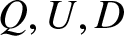 $Q, U, D$ are as follows:
 \begin{equation*}Q = \begin{pmatrix} p_1 & \tilde{p}_3 \\ ip_0 & i\tilde{p}_2
\\ 0 & -\tilde{p}_1 \\ 0 & -i\tilde{p}_0 \end{pmatrix}\,, \quad \qquad
U= \begin{pmatrix} 1 & \textstyle\frac{1}{2b} & \textstyle\frac{1}{(2b)^2} & \textstyle\frac{1}{(2b)^3}\\
0 & 1 & \textstyle\frac{2}{2b} & \textstyle\frac{3}{(2b)^2} \\ 0 & 0 & 1 & \textstyle\frac{3}{2b}\\
0 & 0&0&1\end{pmatrix}\,, \qquad \quad
D= \mathrm{diag} \big(1,\,\,\textstyle\frac{1}{(2b)^2},\,\,\textstyle\frac{1}{(2b)^4}\,\,\textstyle\frac{1}{(2b)^6}\big)\,,
\end{equation*}
where  $\tilde{p}_0=p_0=1, \tilde{p}_1=p_1(\theta_1+h_1),
\tilde{p}_2 = p_2(\theta_1+h_1, \theta_2+h_2)$ with the
 $p_j$ given by (2.7). For
 $n=2$, the index set for the maximal minors
 $\textbf{r}=(r_1 r_2) \in \{(01), (02), (03), (12), (13), (23)\}$, and the
 $2 \times 2$ minors of
 $Q$ are given by
 \begin{equation*}Q(01) =i(p_1\tilde{p}_2-\tilde{p}_3), \,\, Q(02)=-p_1\tilde{p}_1,
\,\, Q(03) =-ip_1, \,\, Q(12) = -i\tilde{p}_1, \,\,
Q(13)=1,\,\, Q(23)=0 \,.\end{equation*}
Note that  $Q(01)$ is a polynomial of degree
 $2(2+1)/2=3$ in
 $\theta_1$ or in the coordinates
 $r,s$, and the other minors
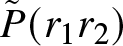 $\tilde{P}(r_1 r_2)$ are of degree
 $(1+3)-(r_1+r_2)$ as mentioned above. The minors of the matrix
 $R=UQ$ are then computed by the Binet–Cauchy formula. For example,
 \begin{align*}
R(01) &= U\tbinom{01}{01} Q(01)+U\tbinom{01}{02}Q(02) +
U\tbinom{01}{03}Q(03)+ U\tbinom{01}{12}Q(12) +
U\tbinom{01}{13}Q(13) \\
& = i(p_1\tilde{p}_2-\tilde{p}_3)-\textstyle\frac{1}{b}p_1\tilde{p}_1
-\textstyle\frac{3i}{4b^2}p_1-\textstyle\frac{i}{4b^2}\tilde{p}_1 + \textstyle\frac{1}{4b^3} \,,
\end{align*}
the remaining  $2 \times 2$ minors of
 $R$ can be obtained in a similar way. One can also verify by using (2.7) to expand the polynomials
 $p_1, \tilde{p}_j, \, j=1,2,3$ in the expression above that
 $R(01)$ depends on only
 $2$ complex parameters namely,
 $\gamma_1$ and
 $\tilde{\gamma}_3=\gamma_3+h_1\gamma_2$. Then from (4.2b)
 \begin{align*}
\det H & = \textstyle\frac{1}{(2b)^2}|R(01)|^2 + \textstyle\frac{1}{(2b)^4}|R(02)|^2 +
\textstyle\frac{1}{(2b)^6}(|R(03)|^2+|R(12)|^2)+\textstyle\frac{1}{(2b)^8}|R(13)|^2 \\
& = \textstyle\frac{1}{(2b)^2} |p_1\tilde{p}_2-\tilde{p}_3 + \textstyle\frac{i}{b}p_1\tilde{p}_1
-\textstyle\frac{1}{b^2}p_1|^2 +
\textstyle\frac{1}{(2b)^4}|p_1\tilde{p}_1+\textstyle\frac{2i}{b}p_1-\textstyle\frac{1}{4b^2}|^2
+\textstyle\frac{2}{(2b)^6}|p_1+\textstyle\frac{i}{2b}|^2 + \textstyle\frac{1}{(2b)^8}
\end{align*}
which is a polynomial of degree  $6$ in
 $r, s$.
In summary, the NSE potential given by (3.4) relates the rational solutions  $\psi(0)$ of the NLS equation (2.14a) to a class of multi-lump solutions of KPI via (2.13). In fact, the NSE (2.1) with the self-consistent potential given by (2.13) is the Lax equation for KPI, and the solution
 $\psi(k)$ given by (2.9) is the corresponding KP eigenfunction associated with this special class of KPI multi-lumps. Furthermore, the NLS solutions depend on
 $n$ arbitrary parameters
 $\gamma_1, \gamma_3, \ldots, \gamma_{2n-1}$, and in particular,
 $\gamma_3$ can be identified with the evolution variable
 $t_3=t$ of the KPI equation (4.1). The remaining parameters may be interpreted as generating symmetries of the multi-lump solutions corresponding to the higher odd flows of the KPI hierarchy.
Remark.
(a) The KPI eigenfunction given by (2.9) or in the form given in Remark (b) at the end of Section 2 is a special case of NSE eigenfunctions investigated using binary Darboux transformation in [Reference Ablowitz, Chakravarty, Trubatch and Villarroel3]. These eigenfunctions are meromorphic in the complex parameter
$k$ with higher-order poles at the eigenvalues
$k=k_0$ and
$\bar{k}_0$. Up to a normalization, these are given by
where
\begin{equation*}\psi(k)=\big[1+\sum_{j=1}^n\frac{\mu_j}{(k-k_0)^j}
+\sum_{j=1}^{m_n-n+1}\frac{\nu_j}{(k-\bar{k}_0)^j}\big]e^{i\theta(k)} \,, \end{equation*}
$m_n \in \mathbb{N}$ and
$\mu_j, \nu_j$ are rational in
$x,y$. In the special case considered here,
$m_n=2n-1$ so that the order of the poles is the same at
$k=k_0$ and
$\bar{k}_0$. Furthermore, the associated potential satisfy the topological relation
where
\begin{equation*} \frac{1}{2\pi i}\int\!\!\!\int_{\mathbb{R}^2}u\mu_1 =
- \frac{1}{2\pi i}\int\!\!\!\int_{\mathbb{R}^2}u\nu_1 = \frac{n(n+1)}{2} \,, \end{equation*}
$\mu_1$ and
$\nu_1$ are, respectively, the residues at the poles
$k=k_0$ and
$k=\bar{k}_0$ of the eigenfunction, and
$n(n+1)/2$ is the degree of the polynomial
$R(\textbf{0})$ (or
$Q(\textbf{0}))$ in the physical coordinates
$r,s \in \mathbb{R}^2$.(b) The KPI equation (4.1) arises as the compatibility condition of the NSE (2.1) and the evolution equation
for
\begin{equation*} \psi_t = -\psi_{xxx}-\textstyle\frac{3}{2}u\psi_x-\textstyle\frac{3}{4}(u_x+iw)\psi, \qquad w_x=u_y \,, \end{equation*}
$\psi=\psi(x,y,t;k)$. Setting
$k=0$ in the above equation and using the transformation
$r=b\psi(0)e^{-2ib^2y}$ together with the expression in (2.13) for the potential
$u$, yields
$r_t-3b^2r_x+r_{xxx}+6|r|^2r_x =0$. Finally, a change of coordinates
$x \to x+3b^2t$ puts the above equation in the standard form of the next member of the NLS hierarchy
\begin{equation*}r_t+r_{xxx}+6|r|^2r_x =0 \,.\end{equation*}Conversely, if
$r(x,y,t)$ satisfies (2.14b) and the above equation then
$u(x,y,t)=2|r|^2$ satisfies the KPI equation (4.1).







4.2. The triangular peak patterns
In this subsection, we will use the theory of KP1 in order to analyse the peak patterns of the NLS lumps. It is useful to note that due to the relation (2.13), the local maxima of  $|\psi(0)|$ for the rational solutions of NLS coincide with those of the NSE potential
 $u$, which are also the multi-lump solutions of KPI. Therefore, it suffices to analyse (3.4) with
 $\det H$ given by (4.2). The resulting expression
 \begin{equation*} u = 2 \partial^2_{xx}\ln \det H = 2\Big(\frac{\partial^2_{xx}\det H}{\det H} -
\frac{(\partial_x \det H)^2}{(\det H)^2}\Big) \end{equation*}
is a nonsingular, rational function of  $x, y$ for fixed values of the
 $n$-parameters
 $\gamma_{2j-1}, \, 1 \leq j \leq n$. Thus,
 $u$ has finitely many local maxima in the
 $xy$-plane, which are complicated to find exactly for
 $n \gt 1$. However, it is possible to find them approximately. The above expression suggests that the local maxima of
 $u$ are near the local minima of
 $\det H$ where
 $\partial_x\det H =0$ and
 $\partial^2_{xx}\det H \gt 0$. Since
 $\det H$ is expressed as a sum of squares in (4.2b), the local minima of
 $\det H$ are located near the points where the leading-order polynomial in this expression given by the maximal minor
 $R(\textbf{0}) =0$. It should be clear from the second equality in (4.2b) and the expression for
 $Q(\textbf{0})$ in (4.3) that
 $R(\textbf{0})$ is a complex polynomial of degree
 $n(n+1)/2$ in the variable
 $\theta_1=i(x+2iby+\gamma_1)$ and depending on the complex parameters
 $\gamma_{2j-1}, \, j=1,\ldots,n$. Hence,
 $R(\textbf{0})$ has
 $n(n+1)/2$ roots in the
 $xy$-plane although some of them may be multiple roots. However, the multiplicity can be broken by choosing the parameters
 $\gamma_{2j-1}$ arbitrarily so that generically speaking,
 $R(\textbf{0})$ has simple roots. Consequently,
 $u$ has
 \begin{equation*} N= \frac{n(n+1)}{2}\end{equation*}
distinct peaks in the  $xy$-plane as were earlier noticed in the examples of Section 3.2.
Next we proceed to estimate the approximate location of the peaks. Note that the leading order term in the expression for the minor  $R(\textbf{0})$ in (4.2b) is the Wronskian function
 $Q(\textbf{0})$ given by the second expression in (4.3), and which depends on the variables
 $\theta_k, \, 1\leq k \leq 2n-1$. By shifting the variables
 $\theta_k \to \theta_k+\delta_k := \tilde{\theta}_k$ it is possible to express
 $R(\textbf{0})$ as a single Wronskian function
 \begin{equation}
R(\textbf{0})(\theta) = Q(\textbf{0}) + \sum_{\textbf{r} \gt \textbf{0}}
U\binom{\textbf{0}}{\textbf{r}}Q(\textbf{r}) = Q(\textbf{0})(\theta+\delta)
= \operatorname{\rm Wr}\nolimits(q_1, q_2, \ldots, q_n)(\theta+\delta)
\end{equation}
using an identity similar to (2.8b) for appropriate choice of  $\delta=(\delta_1, \delta_2, \ldots, \delta_N)$. In particular, it turns out that
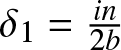 $\delta_1=\textstyle\frac{in}{2b}$. (The reader may consult [Reference Chakravarty and Zowada11] for more details and [Reference Macdonald33] for a proof). Therefore, the approximate location of the peaks is given by the zeros of the Wronskian
 $Q(\textbf{0})$ with shifted argument
 $\tilde{\theta}$ since
 \begin{equation}
R(\textbf{0})(\theta) = 0 \qquad \Rightarrow \quad Q(\textbf{0})(\tilde{\theta}) = 0\,,
\qquad \tilde{\theta} = \theta+\delta \,.
\end{equation}
To determine the peak locations, one solves (4.5) asymptotically for  $\tilde{\theta}_1$ when the parameters satisfy
 $|\gamma_{2j-1}| \gg 1, \, 2 \leq j \leq n$. At first, we will consider the case
 $j=2$, i.e., when
 $|\gamma_3| \gg 1$ and
 $|\gamma_{2j-1}| \sim O(1), \, j \gt 2$. Also, without loss of generality, we set
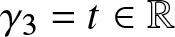 $\gamma_3 = t \in \mathbb{R}$ since it is the time variable for KPI. We will only consider the leading-order estimate for the peak locations below.
Recall from (3.2) that the highest degree generalized Schur polynomial arising in  $q_j$ is
 $p_{2j-1}$. Thus asymptotically as
 $|t| \gg 1$, the leading order contribution to the Wronskian in (4.4) is
 \begin{equation*}Q(\textbf{0})(\tilde{\theta}) = \operatorname{\rm Wr}\nolimits(q_1, q_2, \ldots, q_n)(\tilde{\theta})
\sim \operatorname{\rm Wr}\nolimits(p_1, p_3, \ldots, p_{2n-1})(\tilde{\theta}) \,. \end{equation*}
It can be shown that the  $p_l, \, l \lt 2j-1$ terms in
 $q_j$ contribute to lower order in the asymptotic expansion of
 $Q(\textbf{0})(\tilde{\theta})$. This function
 $\operatorname{\rm Wr}\nolimits(p_1, p_3, \ldots, p_{2n-1})(\tilde{\theta})$ is a special case of the Schur functions which play a fundamental role in the representation theory of symmetric groups. Specifically, it is a weighted homogeneous polynomial in the variables
 $\tilde{\theta}_j$ of degree
 $N=n(n+1)/2$ with weight
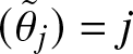 $(\tilde{\theta}_j)=j$, and it is of the form
 \begin{equation}
\operatorname{\rm Wr}\nolimits(p_1,p_3, \ldots p_{2n-1})(\tilde{\theta})
= \sum_{l_j \geq 0} c_N(\textbf{l})\,
\frac{\tilde{\theta}_1^{l_1}\tilde{\theta}_2^{l_2}\cdots\tilde{\theta}_N^{l_N}}
{l_1!l_2! \cdots l_N!}\,, \qquad l_1+2l_2+\cdots+Nl_N=N \,,
\end{equation}
where the coefficients  $c_N(\textbf{l}) \in \mathbb{Z}$ are called the group characters of the symmetric group
 $S_N$ (permutation group of
 $N$ elements), and
 $\textbf{l}=(l_1,l_2,\ldots, l_N)$. Since
 $\theta_j = i\gamma_j, \, j \gt 2$ (cf. (2.6)), the leading order terms in the asymptotic expansion involves only
 $\tilde{\theta}_1$ and
 $\tilde{\theta}_3$ in (4.6) when
 $|t| \gg 1$. These are of the form
 $\tilde{\theta}_1^{l_1}\tilde{\theta}_3^{l_3}$ with
 $l_1+3l_3 = N$. Thus, asymptotically as
 $|t| \gg 1$, the expression for
 $R(\textbf{0})$ in (4.4) reduces to
 \begin{equation*} R(\textbf{0})(\theta) = Q(\textbf{0})(\tilde{\theta}) \sim
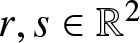
\sum_{l_1,l_3 \geq 0} c_N(\textbf{l})\, \frac{\tilde{\theta}_1^{l_1}\tilde{\theta}_3^{l_3}}
{l_1!l_3!} \,, \qquad \textbf{l} = (l_1, 0, l_3, 0, \ldots, 0)\,, \quad l_1+3l_3 =N \,. \end{equation*}
Since  $N=n(n+1)/2$ is a triangular number, it can always be expressed as either
 $N=3m$ or
 $N=3m+1$ for some
 $m \in \mathbb{N}$. Then the above sum can be re-expressed as
 \begin{equation*}
R(\textbf{0})(\theta) \sim \sum_{r=0}^m c_N(N-3r,3r)
\frac{\tilde{\theta}_1^{N-3r}\tilde{\theta}_3^{r}} {(N-3r)!r!} \,,
\qquad |t| \gg 1\,,
\end{equation*}
Assuming that  $c_N(N,0) \neq 0$ (see below), it is clear that the dominant balance required to asymptotically solve
 $R(\textbf{0}) = 0$ must be
 $\tilde{\theta}_1^N \sim \tilde{\theta}_1^{N-3r}\tilde{\theta}_3^r$ so that
 $\tilde{\theta}_1 \sim |t|^{1/3}$ for
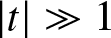 $|t| \gg 1$. Using the coordinates
 $r,s$ introduced in Section 3.2 one can set
 \begin{equation*}\tilde{\theta}_1=iz, \,\, z=r+\delta_1+is+\gamma_1, \,\,
\tilde{\theta}_3=i(t+\delta_3) \sim it\,, \quad z=(\textstyle\frac{t}{a})^{1/3}(\xi+O(t^{-1/3}))\end{equation*}
where  $\delta_1 = \textstyle\frac{n}{2b}$ (see above (4.5)),
 $z$ is rescaled using the dominant balance
 $z \sim O(t^{1/3})$, and
 $a \neq 0$ is a constant to be determined later. Then the above asymptotic expression of
 $R(\textbf{0})$ takes the form
 \begin{equation}
R(\textbf{0}) (r,s,t) \sim
i^N(t/a)^{N/3}\Big[\frac{c(N,0)}{N!}\,Q_n(\xi)+O(t^{-1/3})\Big]\,,
\end{equation}
where  $Q_n(\xi)$ is a monic polynomial of degree
 $N=n(n+1)/2$, which can be identified with the well-known Yablonskii–Vorob’ev polynomials as follows.
The leading order contribution to the Wronskian  $\operatorname{\rm Wr}\nolimits(p_1,p_3,\ldots, p_{2n-1})$ as
 $|t| \gg 1$, may be calculated from
 \begin{equation*}
p_r(\tilde{\theta}) \sim p_r(\tilde{\theta}_1, 0,\tilde{\theta}_3, 0, \ldots, 0)
\sim p_r(iz, 0, it, 0, \ldots, 0) = i^r\Big(\frac{t}{a}\Big)^{r/3}\, S_r(\xi,a) \,,
\end{equation*}
and after rescaling  $z$ as above. It follows from the definition of the generalized Schur polynomials in (2.7) that
 \begin{equation*}
S_r(\xi,a)= \sum_{k,l \geq 0}\frac{\xi^k (-a)^l}{k!l!}, \quad k+3l=r\,, \qquad
\exp(\lambda \xi-\lambda^3 a) = \sum_{r=0}^\infty S_r(\xi, a)\lambda^r\,.
\end{equation*}
Then the leading order term in  $\operatorname{\rm Wr}\nolimits(p_1,p_3,\ldots,p_{2n-1})$ when
 $|t| \gg 1$, corresponds to the first term in (4.7) with
 \begin{equation*}\operatorname{\rm Wr}\nolimits(S_1,S_3,\ldots,S_{2n-1}) = \frac{c(N,0)}{N!}\,Q_n(\xi)\,, \quad \quad
\frac{c(N,0)}{N!} = \Big(\prod_{j=1}^n(2j-1)!!\Big)^{-1} \,. \end{equation*}
Finally, choosing the constant  $a=\textstyle\frac{4}{3}$, the resulting polynomial
 $Q_n(\xi)$ has integer coefficients and coincides with the Yablonskii–Vorob’ev polynomials which were originally studied to obtain special rational solutions of the second Painlevé equation PII [Reference Vorob’ev41, Reference Yablonskii43]. These are of the form
 \begin{equation*} Q_n(\xi)= \xi^{N-3m}\sum_{r=0}^m (-\textstyle\frac{4}{3})^rc_r\xi^{3(m-r)} \,,
\qquad m=\left\{\begin{matrix} \textstyle\frac{N}{3} \,, & \quad N=3m \\
\textstyle\frac{N-1}{3} \,, & \quad N=3m+1 \end{matrix} \right. \,,
\end{equation*}
where the coefficients  $c_r$ are given in terms of the group characters
 $c(N-3r, r)$. These polynomials can also be obtained recursively from a nonlinear differential-difference system [Reference Vorob’ev41, Reference Yablonskii43] and are known to have
 $N$ distinct roots in the complex plane [Reference Fukutani, Okamoto and Umemura19]. The first few Yablonskii–Vorob’ev polynomials are given by
 \begin{equation*} Q_0 = 1, \quad Q_1=\xi, \quad Q_2=\xi^3+4, \quad Q_3=\xi^6+20\xi^3-80, \ldots \,.\end{equation*}
The roots of  $Q_n(\xi)$ are either real or complex conjugate pairs. Moreover, the roots are arranged in the complex plane in a ‘triangular’ pattern due to the symmetry:
 $\xi \to \xi e^{2\pi i/3}$ since
 $Q(\xi)$ can be expressed as
 $Q(\xi) = \xi^{N-3m}P_m(\xi^3)$ where
 $P_m$ is a polynomial of degree
 $m$ with respect to its argument. There exists an extensive literature on the Yablonskii–Vorob’ev polynomials and patterns of its roots in the complex plane (see, e.g., [Reference Clarkson and Mansfield13] and references therein). They arise as the Painlevé II reductions of the rational solutions of the KdV and modified KdV equations [Reference Kajiwara and Ohta26], hence it is natural for them to appear in the context of the rational solutions of KPI (see Remark (b) below).
Note that the  $O(t^{-1/3})$ term in (4.7) arises from all the subdominant terms in
 $R(\textbf{0})(\theta)$ after the rescaling
 $z(t) \sim O(t^{1/3})$. These arise from the lower degree generalized Schur polynomials neglected in the approximation
 $q_j \approx p_{2j-1}$ for the Wronskian in (4.4). Additionally, the terms in (4.6) that are not of the form
 $\tilde{\theta}_1^{l_1}\tilde{\theta}_3^{l_3}$ also contribute to the subdominant terms. Setting
 $R(\textbf{0})(r,s,t)=0$ in (4.7), one can solve for
 $\tilde{\theta}_1 =iz(t)$ asymptotically for
 $|t| \gg 1$ as
 \begin{equation*}z(t) = (\textstyle\frac{t}{a})^{1/3}(\xi + \epsilon z_1 + \epsilon^2 z_2 + \cdots)\,,
\qquad \epsilon = t^{-1/3} \,, \end{equation*}
to obtain  $\xi=\xi_j$ where
 $\xi_j$ is a root of
 $Q_n(\xi)=0$. Thus the leading-order approximation to the locations of the NLS and KPI
 $N$-lump peaks for
 $|t| \gg 1$ are obtained as
 \begin{equation}
z_j(t):= r_j(t) + is_j(t) = (r_0-\textstyle\frac{n}{2b} + is_0)+
(\textstyle\frac{3}{4}t)^{1/3}\big(\xi_j+O(t^{-1/3})\big)\,, \qquad j=1,2, \ldots, N \,,
\end{equation}
where  $r_0+is_0 = -\gamma_1$.
If  $n=3k+1$ for some
 $k \in \mathbb{N}$ then
 $Q_n(\xi)$ has a root at
 $\xi=0$ with multiplicity
 $1$. In this case,
 $N=3m+1$ for some
 $m \in \mathbb{N}$, and there is a single term in the Wronskian in (4.6) of the form
 $\tilde{\theta}_1\tilde{\theta}_3^m$ that dominates when
 $|t| \gg 1$. Rearranging all terms in the Wronskian in descending power of
 $\tilde{\theta}_3$, one finds that (4.5) admits one asymptotic solution
 $\tilde{\theta}_1 \sim 0 + O(t^{-1})$ which implies that the approximate peak location
 \begin{equation*} z(t) \sim (r_0-\textstyle\frac{3k+1}{2b}+is_0) + O(t^{-1}) \,.\end{equation*}
This is the case which corresponds to the  $\xi=0$ root of
 $Q_n(\xi)$. The first non-trivial solution of this type corresponding to
 $k=1$, i.e.,
 $n=4$ is shown below in Figure 4. The simplest triangular lump solution corresponds to
 $n=2, \, N=3$ which was also discussed earlier in Section 3.2 and in the example given in Section 4.2. Figure 4 compares the exact and the approximate peak locations given by (4.8) for the cases
 $n=3,4,5$ corresponding to
 $N=6, 10, 15$, respectively. Recall from (2.13) that these also correspond to the peak locations of
 $|\psi(0)|^2$ of the NLS solution in (2.14a) where
 $t$ is a parameter.
Triangular lump peak locations for 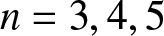 $n=3,4,5$ at
 $t=-40$ (top panel) and
 $t=40$ (bottom panel). Total number of peaks
 $N=\textstyle\frac{n(n+1)}{2}$ (see text). Black dots represent locations
 $z_j$ where
 $R(\textbf{0})=0$, red open circles are exact locations. Under time reversal (
 $t \to -t$), the peak locations are reflected across the dashed vertical line:
 $r=-\textstyle\frac{n}{2b}$. Parameters:
 $b=1$ and
 $\gamma_3 =t, \gamma_j=0, \, j \neq 3$.

Figure 4 Long description
A scatter plot with the text, t equals minus 40. The horizontal axis is labeled, r, with tick labels at negative 10, negative 5, 5. The vertical axis is labeled, s, with tick labels at negative 5 and 5. A dashed vertical line is drawn slightly left of the vertical axis. Plotted points appear near left side around r near negative 10 and s near 7, around r near negative 6 and s near 0, around r near negative 8 and s near negative 7, around r near 1 and s near 4, around r near 1 and s near negative 4 and around r near 8 and s near 0. The points form three vertical groupings around r near negative 10, r near 1 and r near 8. The image B showing a scatter plot with the text, t equals minus 40. The horizontal axis is labeled, r, with tick labels at negative 15, negative 10, negative 5, 5, 10. The vertical axis is labeled, s, with tick labels at negative 10, negative 5, 5, 10. A dashed vertical line is drawn slightly left of the vertical axis. Plotted points appear near r near negative 10 and s near 10, r near negative 10 and s near 3, r near negative 9 and s near negative 2, r near negative 8 and s near negative 9, r near 0 and s near 0, r near 0 and s near 7, r near 0 and s near negative 7, r near 4 and s near 4, r near 4 and s near negative 3 and r near 10 and s near 0. The points form groups around r near negative 10, r near 0, r near 4 and a single point near r near 10. The image C showing a scatter plot with the text, t equals minus 40. The horizontal axis is labeled, r, with tick labels at negative 20, negative 15, negative 10, negative 5, 5, 10, 15. The vertical axis is labeled, s, with tick labels at negative 15, negative 10, negative 5, 5, 10, 15. A dashed vertical line is drawn slightly left of the vertical axis. Plotted points appear near r near negative 12 and s near 13, r near negative 10 and s near 6, r near negative 10 and s near 0, r near negative 10 and s near negative 6, r near negative 10 and s near negative 13, r near negative 5 and s near 10, r near negative 5 and s near 2, r near negative 5 and s near negative 2, r near negative 5 and s near negative 10, r near 0 and s near 7, r near 0 and s near 0, r near 0 and s near negative 7, r near 6 and s near 4, r near 6 and s near negative 3 and r near 14 and s near 0. The points form multiple vertical groupings around r near negative 10, r near negative 5, r near 0, r near 6 and a single point near r near 14. The image D showing a scatter plot with the text, t equals 40. The horizontal axis is labeled, r, with tick labels at negative 10, negative 5, 5. The vertical axis is labeled, s, with tick labels at negative 5 and 5. A dashed vertical line is drawn slightly left of the vertical axis. Plotted points appear near r near negative 10 and s near 0, r near negative 6 and s near 4, r near negative 5 and s near negative 3, r near 2 and s near 0, r near 3 and s near 7 and r near 3 and s near negative 7. The points form groupings around r near negative 10, r near negative 6 to negative 5, r near 2 and r near 3. The image E showing a scatter plot with the text, t equals 40. The horizontal axis is labeled, r, with tick labels at negative 15, negative 10, negative 5, 5, 10. The vertical axis is labeled, s, with tick labels at negative 10, negative 5, 5, 10. A dashed vertical line is drawn slightly left of the vertical axis. Plotted points appear near r near negative 15 and s near 0, r near negative 10 and s near 3, r near negative 9 and s near negative 3, r near 0 and s near 0, r near 0 and s near 7, r near 0 and s near negative 7, r near 4 and s near 10, r near 4 and s near 4, r near 4 and s near negative 3 and r near 4 and s near negative 10. The points form groupings around r near negative 15, r near negative 10, r near 0 and r near 4. The image F showing a scatter plot with the text, t equals 40. The horizontal axis is labeled, r, with tick labels at negative 20, negative 15, negative 10, negative 5, 5, 10, 15. The vertical axis is labeled, s, with tick labels at negative 15, negative 10, negative 5, 5, 10, 15. A dashed vertical line is drawn slightly left of the vertical axis. Plotted points appear near r near negative 16 and s near 0, r near negative 12 and s near 3, r near negative 10 and s near negative 3, r near negative 6 and s near 0, r near 0 and s near 10, r near 0 and s near 4, r near 0 and s near negative 4, r near 0 and s near negative 10, r near 4 and s near 12, r near 4 and s near 7, r near 4 and s near 0, r near 4 and s near negative 7, r near 4 and s near negative 12 and r near 14 and s near 0. The points form groupings around r near negative 16, r near negative 12 to negative 10, r near negative 6, r near 0, r near 4 and a single point near r near 14. Across the six scatter plots, the dashed vertical line appears in each plot at a similar r position slightly left of the vertical axis. The number of plotted points increases from image A to image C and from image D to image F.
Remark.
(a) It should be emphasized that (4.8) gives the approximate locations of the triangular
$N$-lump solutions. The absolute difference between the exact and approximate locations is
$O(|t|^{-1/3})$ when
$\xi_k \neq 0$ and
$O(|t|^{-1})$ when
$\xi_k = 0$, for
$|t| \gg 1$.(b) The Painlevé II reduction of the KPI equation (4.1) in fact corresponds to a
$2$-reduction of the KP hierarchy to KdV and then to Painlevé II via a similarity transformation. First one sets
$u(x,y,t) = u(z,t)$ in (4.1) with
$z = r+is, r=x-3b^2t, s=2by$ to obtain the complex KdV equation
\begin{equation*} 4u_t + u_{zzz} + 6uu_z =0 \,.\end{equation*}Next, the similarity reduction
yields the equation
\begin{equation*}u(z,t)= b t^{-2/3}v(\xi)\,, \qquad \xi=azt^{-1/3}\,, \quad a=(-4/3)^{1/3}\,,
\quad b=a^2 \end{equation*}for the function
\begin{equation*} v^{\prime\prime\prime} + 6vv' - (2v + \xi v') \end{equation*}
$v(\xi)$. Finally, the invertible Miura transformation [Reference Fokas and Ablowitz18]
leads to the Painlevé II equation:
\begin{equation*} v = -( w'+w^2)\,, \qquad \quad w = \frac {v'+\alpha}{2v-\xi} \end{equation*}
$w''=2w^3+\xi w + \alpha$ whose rational solutions exist when the constant
$\alpha = n \in \mathbb{Z}$. In particular, if
$n \in \mathbb{N}$ the rational solutions are unique and are given in terms of the Yablonskii–Vorob’ev polynomials as
$w(\xi,n) = \partial_\xi\ln(Q_{n-1}/Q_n)$ [Reference Clarkson and Mansfield13].(c) The leading-order approximate peak locations is also governed by a well-known dynamical system studied in [Reference Airault, McKean and Moser6]. It can be shown that the Wronskian
$\tau(z,t)=\operatorname{\rm Wr}\nolimits(p_1,p_3,\ldots,p_{2n-1})$ constructed from the reduced Schur polynomials
$p_n = p_n(z,t)$ defined below (4.7), solves the complex KdV equation (see Remark (b)) with
$u(z,t)=2(\ln \tau)_{zz}$. The polynomials
$\tau(z,t)$ for
$n \in \mathbb{N}$ are the Adler-Moser polynomials [Reference Adler and Moser5] which are known to have
$N=n(n+1)/2$ distinct roots. Substituting
$\tau(z,t) = (z-z_1(t))(z-z_2(t))\cdots(z-z_N(t))$ back into the KdV equation it is possible to deduce a first-order dynamical system for the roots
$z_j(t)$ together with constraints, namely
which were found in [Reference Airault, McKean and Moser6].
\begin{equation*}z_{jt} = \sum_{i \neq j}\frac{3}{(z_j-z_i)^2}\,, \quad \qquad
\sum_{i=1, i \neq j}^N\frac{1}{(z_j-z_i)^3}=0\,, \quad j=1,2,\ldots,N \,,\end{equation*}


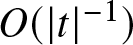











4.3. General peak patterns
The procedure outlined in Section 4.2 can be extended to determine the peak locations and associated patterns in the  $rs$-plane for the function
 $u(r,s; \gamma_1, \gamma_3, \ldots, \gamma_{2n-1})$ asymptotically as
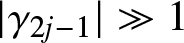 $|\gamma_{2j-1}| \gg 1$ for any fixed
 $j \gt 2$, and where the magnitudes of the remaining parameters are
 $O(1)$. The resulting patterns are not triangular as for the
 $j=2$ case but vary with each
 $j$. For conveninence we set
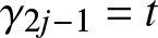 $\gamma_{2j-1} = t$ as in Section 4.2. Then as
 $|t| \gg 1$, the leading order behaviour of
 $R(\textbf{0})$ using (4.6) is obtained as
 \begin{equation*} R(\textbf{0})(\theta) = Q(\textbf{0})(\tilde{\theta}) \sim
\sum_{l_1,l_{2j-1} \geq 0} c_N(l_1,l_{2j-1})\,
\frac{\tilde{\theta}_1^{l_1}\tilde{\theta}_{2j-1}^{l_{2j-1}}}
{l_1!l_{2j-1}!} \,, \quad \quad l_1+(2j-1)l_{2j-1} =N \end{equation*}
since  $\theta_{2j-1} = i\gamma_{2j-1}$. Proceeding as in Section 4.2, one sets
 \begin{equation*}{\widetilde\theta}_1=iz,\,\,z=r+{\textstyle\frac n{2b}+is+\gamma_1,\,\,{\widetilde\theta}_{2j-1}=i(t+\delta_{2j-1})\sim it\,,\quad z=(\frac t{a_j})^{1/(2j-1)}(\xi+O(t^{-1/(2j-1)}))}\end{equation*}
where  $a_j$ is a constant to be determined later. Substituting these into the expression for
 $R(\textbf{0})$ above, yields
 \begin{equation}
R_j(\textbf{0}) (r,s,t) \sim
i^N(t/a_j)^{N/(2j-1)}\Big[\frac{c(N,0)}{N!}\,Q^{[j]}_n(\xi)+O(t^{-1/(2j-1)})\Big]\,,
\end{equation}
where 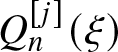 $Q^{[j]}_n(\xi)$ is a monic polynomial of degree
 $N=n(n+1)/2$ and is regarded as the
 $j^{\mathrm th}$-order Yablonskii–Vorob’ev polynomial with suitable choice of the scaling parameter
 $a_j$. The polynomial
 $Q^{[j]}_n(\xi)$ is derived from the Wronskian form
 $Q(\textbf{0})(\tilde{\theta}) \sim \operatorname{\rm Wr}\nolimits(p_1,p_3,\ldots, p_{2n-1})$ whose asymptotic form for
 $|\gamma_{2j-1}|=|t| \gg 1$ is obtained by taking
 \begin{equation*} p_r \sim p_r(\tilde{\theta}_1, 0, \ldots, 0, \tilde{\theta}_{2j-1}, 0, \ldots, 0)
\sim p_r(iz, 0, \ldots, it, 0, \ldots, 0) =
i^r\Big(\frac{t}{a_j}\Big)^{r/{(2j-1)}}\,S^{[j]}_r(\xi,a_j) \end{equation*}
after rescaling  $z=(t/a_j)^{1/(2j-1)}\xi$. The reduced Schur polynomials
 $S^{[j]}_r(\xi,a_j)$ are given by
 \begin{equation*}
S^{[j]}_r(\xi,a_j)= \sum_{k,l \geq 0}\frac{\xi^k ((-1)^{j-1}a_j)^l}{k!l!},
\quad k+(2j-1)l=r\,, \qquad \exp(\lambda \xi+\lambda^{2j-1} (-1)^{j-1}a_j) =
\sum_{r=0}^\infty S^{[j]}_r(\xi, a_j)\lambda^r\,.
\end{equation*}
Then to leading order
 \begin{equation*}\operatorname{\rm Wr}\nolimits(p_1,p_3,\ldots,p_{2n-1})
\sim i^N(t/a_j)^{N/(2j-1)} \operatorname{\rm Wr}\nolimits(S^{[j]}_1,S^{[j]}_3,\ldots,S^{[j]}_{2n-1}) \end{equation*}
from which one can recover the expression for  $Q_n^{[j]}(\xi)$ as
 \begin{equation*} Q^{[j]}_n(\xi)= \xi^{s_j}\sum_{r=0}^m ((-1)^{j-1}a_j)^rc_r\xi^{(2j-1)(m-r)} \,,
\quad \qquad c_r = \frac{c(N-(2j-1)r,r)N!}{c(N,0)(N-(2j-1)r)!r!}\,. \end{equation*}
Here the coefficients  $c_r$ are related to the characters of the symmetric group and the non-negative integers
 $s_j$ and
 $m$ are determined by (long division)
 \begin{equation*} N = (2j-1)m + s_j\,, \quad s_j \in \{0,1,\ldots,2j-2\} \qquad \Longleftrightarrow \quad
N \equiv s_j \,\, \text{mod} \,\, 2j-1 \,,\end{equation*}
i.e.,  $s_j$ is the residue of
 $N$ modulo
 $2j-1$. Finally, if one sets
 $a_j=4^{j-1}/(2j-1)$, the corresponding polynomials
 $Q^{[j]}_n(\xi)$ are the
 $j \gt 2$ extensions of the Yablonskii–Vorob’ev polynomials as they are also associated with the rational solutions of the Painlevé II hierarchy [Reference Clarkson and Mansfield13]. For
 $j=2$,
 $Q^{[2]}_n(\xi) = Q_n(\xi)$ are the usual Yablonskii–Vorob’ev polynomials.
Recall that for  $2j-1=3$,
 $N=3m, 3m+1$, i.e.,
 $s_2 \in \{0,1\}$ and
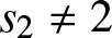 $s_2 \neq 2$ so that the Yablonskii–Vorob’ev polynomials have at most one root at
 $\xi=0$. However, for
 $j \gt 2$, the exact set of residues
 $N \equiv s_j$ mod
 $2j-1$ for triangular numbers
 $N=n(n+1)/2, \, n \in \mathbb{N}$ can not be enumerated in a simple way to the best of the author’s knowledge. If
 $n \equiv r$ mod
 $2j-1$ then
 $N=n(n+1)/2 \equiv r(r+1)/2$ mod
 $2j-1$. Hence, the residue
 $s_j$ can be found by only considering the values
 $0 \leq r \leq 2j-2$. Furthermore, the residues corresponding to
 $r=j-1+k$ and
 $r=j-1-k$ for
 $0 \leq k \leq j-1$ are the same. Thus it suffices to check the residues
 $r(r+1)/2$ mod
 $2j-1$ only for the values
 $0 \leq r \leq j-1$ in order to obtain the full set of
 $s_j$ for any given
 $j$. For example, when
 $j=3$, i.e.,
 $2j-1=5$, the possible residues
 $s_3=0,1,3$ which are obtained by considering
 $r=0,1,2$. Similarly,
 $s_4=0,1,3,6$,
 $s_5=0,1,3,6$ and so on. The upshot is that the
 $Q^{[j]}_n(\xi)$ has a root at
 $\xi=0$ of multiplicity
 $s_j \gt 1$ depending on the value of
 $n$. As for the roots at
 $\xi \neq 0$, it was conjectured in [Reference Clarkson and Mansfield13] that they are simple.
The peak locations for the lump solution  $u(r,s,t)$ and
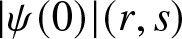 $|\psi(0)|(r,s)$ for
 $|t| \gg 1$ is given in a similar way as in (4.8) from the expansion
 $z(t)=({\textstyle\frac t{a_j})^{1/(2j-1)}(\xi+\epsilon z_1+\epsilon^2z_2+\cdots), \,\,\epsilon=t^{-1/(2j-1)}.}$One obtains that
 \begin{equation}z_p(t):=r_p\left(t\right)+is_p\left(t\right)=\left(r_{0}-\frac{n}{2b}+is_{0}\right)+\left(\frac{t}{a_{j}}\right)^{1/(2j-1)}(\xi_{p}+O(t^{-1/(2j-1)}))\,,\qquad p=1,2,\dots,N-s_j\,,\end{equation}
corresponding to the roots  $\xi_p \neq 0$ for the polynomials
 $Q^{[j]}_n(\xi)$, assuming that they are simple. The peak locations in the
 $rs$-plane scale as
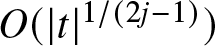 $O(|t|^{1/(2j-1)})$ and are separated for large values of
 $|t|$. The peak patterns approximately follow the distribution of the zeros of the
 $Q^{[j]}_n(\xi)$ which exhibit the symmetry
 $\xi \to \xi e^{2\pi i/(2j-1)}$ in the complex plane since
 $Q^{[j]}_n(\xi)=\xi^{s_j}P^{[j]}(\zeta), \, \zeta=\xi^{2j-1}$. For each root
 $\zeta_r, \, 1 \leq r \leq m$ of
 $P^{[j]}(\zeta)$, there are
 $2j-1$ roots
 $\xi_i^{(r)}, \, 1 \leq i \leq 2j-1$ of
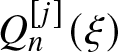 $Q^{[j]}_n(\xi)$ arranged
 $2\pi/(2j-1)$ apart on a circle around the origin of radius
 $|\zeta_r|$.
The peak locations corresponding to the  $\xi=0$ roots of
 $Q^{[j]}_n(\xi)$ are obtained as in the triangular case of Section 4.2. In this case, arranging the terms in the Wronskian of (4.6) in descending powers of
 $\tilde{\theta}_{2j-1}$, one finds that the term corresponding to highest power of
 $\tilde{\theta}_{2j-1}$ is
 $\tilde{\theta}_1^{s_j}\tilde{\theta}_{2j-1}^m, \,
m=(N-s_j)/(2j-1)$. Then (4.5) implies that there is an asymptotic solution of the form
 $\tilde{\theta}_1^{s_j} \sim 0 + O(t^{-1}), \, \tilde{\theta}_{2j-1} \sim it$. This leads to the peak locations
 \begin{equation}
z_p(t):= r_p(t) + is_p(t) = (r_0-\textstyle\frac{n}{2b} + is_0)+O(t^{-1})\,, \quad
p=1,2, \ldots, s_j \,, \quad |t| \gg 1 \,.\end{equation}
Thus  $z_p \sim O(1)$ and they are all located within a
 $O(|t|^{-1})$ neighbourhood, and it is necessary to retain the
 $O(t^{-1})$ term (which depends on the lower order terms contributing to
 $R(\textbf{0})$ in (4.4) and the parameters
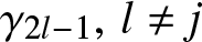 $\gamma_{2l-1}, \, l \neq j$) in order to distinguish them.
 $6$-lump solutions of the NLS equation. Parameters:
 $\gamma_1=\gamma_2=0=\gamma_3 = 0, \gamma_5=4000, b=\textstyle\frac12$. Left panel:
 $|\psi(0)|$, right panel:
 $u$.

 $6$-lump solutions of the NLS equation. Parameters:
 $\gamma_1=\gamma_2=\gamma_3 = 0, \gamma_5=4000, b=1$. Black dots represent locations
 $z_p$ where
 $R_3(0)=0$, red open circles are exact locations. Notice that the central peak is located on the
 $r$-axis near
 $r=-\textstyle\frac{n}{2b}$ with
 $n=3$, as prescribed by the asymptotic estimate (4.10b).

The special case of the  $6$-lump solution and the corresponding peak locations for large
 $|\gamma_5|$ (i.e.,
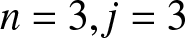 $n=3, j=3$) are shown in Figures 5 and 6. Unlike the triangular patterns in Figures 3 and 4, these
 $6$-lump solutions form a pentagonal pattern in the
 $rs$-plane with a single peak at the centre of the pattern near the origin. The central peak appears since
 $N=6 \equiv 1$ mod
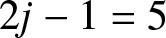 $2j-1=5$ so that the residue
 $s_2=1$. Figure 6 shows both the exact peak locations as well as the estimated values obtained from (4.10) solving for
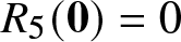 $R_5(\textbf{0})=0$ asymptotically as
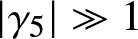 $|\gamma_5| \gg 1$. The peak locations near the vertices of the pentagon correspond to the non-zero roots of the polynomial
 $Q^{[3]}_3(\xi)=\xi(\xi^5 -144)$.
Next we consider the case of  $n=4$, which corresponds to a
 $10$-lump solution depending on the parameters
 $\{\gamma_1,\gamma_3,\gamma_5,\gamma_7\}$. The peak locations for this case when
 $|\gamma_3| \gg 1$ and the remaining parameters are
 $O(1)$ was already illustrated in Figure 4. Here, we depict the peak patterns when (i)
 $|\gamma_5| \gg 1$ and (ii)
 $|\gamma_7| \gg 1$ and the remaining parameters are
 $O(1)$ in each subcase. For the first subcase,
 $j=3$. Setting
 $R_3(\textbf{0})=0$ in (4.9), the leading-order peak locations are given in terms of the roots of the polynomial
 $Q^{[3]}_4(\xi)=\xi^{10}-1008\xi^5 -48384$. Note that
 $Q^{[3]}_4(\xi)$ has no roots at
 $\xi=0$ since
 $10$ is divisible by
 $2j-1=5$ and also that
 $Q^{[3]}_4(\xi) = P^{[3]}(\zeta), \, \zeta=\xi^5$. Since
 $P^{[3]}(\zeta)$ is quadradic in
 $\zeta$ with non-zero roots
 $\zeta_1, \zeta_2$, Figure 7 shows that the
 $10$ peaks are arranged in
 $2$ sets of pentagonal pattern spaced
 $2 \pi/5$ apart on circles of radii
 $|\zeta_1|$ and
 $|\zeta_2|$ around the origin in the
 $rs$-plane. These peak locations are obtained from (4.10a).
The second subcase corresponding to  $j=4$ and
 $|\gamma_7| \gg 1$ is more interesting, and is obtained asymptotically from
 $R_4(\textbf{0})=0$ in (4.9). Since
 $10 \equiv 3$ mod
 $7$, i.e.,
 $s_4=3$, there are
 $3$ peaks located near the origin as shown in Figure 8. These peaks correspond to the
 $\xi=0$ roots of multiplicity
 $3$ for the polynomial
 $Q^{[4]}_4(\xi) = \xi^3(\xi^7+14400)$ and the locations are given by (4.10b). Note that the peaks form a triangular pattern near the origin. This stems from considering the subdominant
 $O(t^{-1})$ terms in (4.10b) with the parameter
 $\gamma_3 \sim O(1)$. We do not pursue the analysis here. The remaining
 $7$ peaks are arranged
 $2 \pi/7$ apart on a circle around the origin, and their locations are given to leading order by (4.10a) for
 $|\gamma_7| \gg 1$.
 $10$-lump peak locations of the NLS equation. Parameters:
 $\gamma_j=0,\, 1 \leq j \leq 4, \gamma_5=10000, \gamma_6=\gamma_7=0, b=\textstyle\frac12$. Left panel:
 $|\psi(0)|$, right panel:
 $u$. The peaks are arranged in
 $2$ sets of pentagonal pattern given by (4.10a).

 $10$-lump solutions of the NLS equation. Parameters:
 $\gamma_j=0$ except for
 $\gamma_3=10, \gamma_7=10^6, b=\textstyle\frac{1}{2}$. Black dots represent locations
 $z_p$ where
 $R_4(0)=0$, red open circles are exact locations. Notice that the
 $3$ peaks near the centre form a triangular pattern due to
 $\gamma_3 \neq 0$. These locations can be obtained from further asymptotic estimate of the
 $O(t^{-1})$ term in (4.10b).

Remark.
(a) The scaling
$z(t) \sim O(t^{1/(2j-1)})$ to derive the asymptotic form of
$R_j(\textbf{0})$ in (4.9) makes sense only when
$\tilde{\theta}_{2j-1}$ is present in the Wronskian function
$\operatorname{\rm Wr}\nolimits(p_1,p_3, \ldots, p_{2j-1}, \ldots, p_{2n-1})$ of (4.6). That is, the peak locations in (4.10a) and (4.10b) corresponding to the roots of
$Q^{[j]}_n(\xi)$ are valid only when
$j \leq n$ even though these polynomials are defined for
$j \gt n$. For example, in the triangular case with
$j=2$, the first nontrivial example corresponds to the
$3$-lump solutions with
$n=2$ even though the Yablonskii–Vorobév polynomials
$Q_0=1, Q_1=\xi$ are well defined. Similarly, when
$j=3$ the polynomials
$Q^{[3]}_0(\xi)=1, Q^{[3]}_1(\xi)=\xi, Q^{[3]}_2(\xi)=\xi^3$ do not contribute to determine the peak locations of any of the
$N$-lump solutions. The first non-trivial case corresponds to
$Q^{[3]}_3=\xi(\xi^5 -144)$ which gives rise to the pentagonal peak patterns of a
$6$-lump solution when
$|\gamma_5| \gg 1$ as shown in Figures 5 and 6.(b) The earliest non-trivial case when the root at
$\xi=0$ for
$Q^{[j]}_n(\xi)$ is of multiplicity
$s_j \gt 1$, corresponds to
$j=4$ and
$n=4$. In this case, the residue
$s_4=3$. The associated
$N=10$-lump solution with
$3$ of the lump peaks in the centre of the
$rs$-plane for
$|\gamma_7| \gg 1$ is illustrated in Figure 8. Note that the residues
$s_j \gt 1$ are not necessarily triangular numbers as claimed in [Reference Yang and Yang45]. For example, if
$j=6$ and
$n=16 \gt j$ so that
$R_6(\textbf{0})=0$ yields asymptotic estimates of the peak locations then
$N=136 \equiv 4$ mod
$11$ but
$s_6=4$ is not triangular.(c) The rational solution
$\psi(0)(r,s,\gamma_{2j-1})$ of (2.14a) and in particular the NLSE potential
$u(r,s, \gamma_{2j-1})$ for
$|\gamma_{2j-1}| \gg 1, \, j \gt 2$ can be viewed as rational solutions of the complex KdV hierarchy if
$\gamma_{2j-1} := t_{2j-1} \in \mathbb{R}$ is identified with an evolution variable. It is well known that the associated KPI hierarchy of which (4.1) is the first member admits a
$2$-reduction to the KdV hierarchy for odd time variables
$(t_1=x, t_3, t_5, \ldots)$. Indeed, by setting
the solution
\begin{equation*}z=r+is\,, \quad r=x-(-1)^j(2j-1)b^{2j-2}t_{2j-1} \,, \quad s=2by \,, \end{equation*}
$u(r,s,t_{2j-1})$ for
$|t_{2j-1}| \gg 1$ satisfies the KdV hierarchy for
$u(z,t_{2j-1})$, namely
\begin{equation*}u_{t_{2j-1}}+ L^{j-1}(u_z)=0 \,, \qquad L=\partial_{zz}+4u+2u_z\partial_z^{-1}\,,
\quad j \gt 2\,. \end{equation*}The scaling reduction of the above equation (after a Miura transformation to the modified KDV hierarchy) leads to the PII-hierarchy (see, e.g., [Reference Clarkson and Mansfield13]).





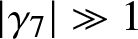


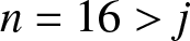







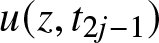

5. Concluding remarks
In this paper, the properties of the NSE with a special class of self-consistent rational potentials have been investigated. It is shown that the NSE wavefunctions in this case satisfy the NLS equation and correspond to particular rational solutions which have been studied to describe the rogue wave phenomena in water waves and optics. The NLS solutions are also shown to correspond to the eigenfunctions associated with a special class of multi-lump solutions of the KPI equation by suitably interpreting the parametric dependence of these solutions as ‘time’-dependence of the KPI eigenfunction. This correspondence was pointed out in earlier papers using algebro-geometric methods [Reference Dubard, Gaillard, Klein and Matveev14, Reference Dubard and Matveev15] which are somewhat esoteric. In contrast, the current work utilizes much simpler algebraic techniques which guarantee that the underlying solutions are non-singular in physical coordinates.
It appears that the methods described in this paper may be applied to study rational solutions of other nonlinear equations that can be derived from the NSE with different types of self-consistent potentials. It would be interesting to pursue such questions in the future, and explore the underlying connection with possibly other classes of KPI eigenfunctions.
Acknowledgements
S.C. thanks Professor Mark Ablowitz (CU Boulder) for numerous insightful discussions on KPI lumps and properties of associated NSE eigenfunctions. This article is dedicated to Mark on the occasion of his 80th birthday.
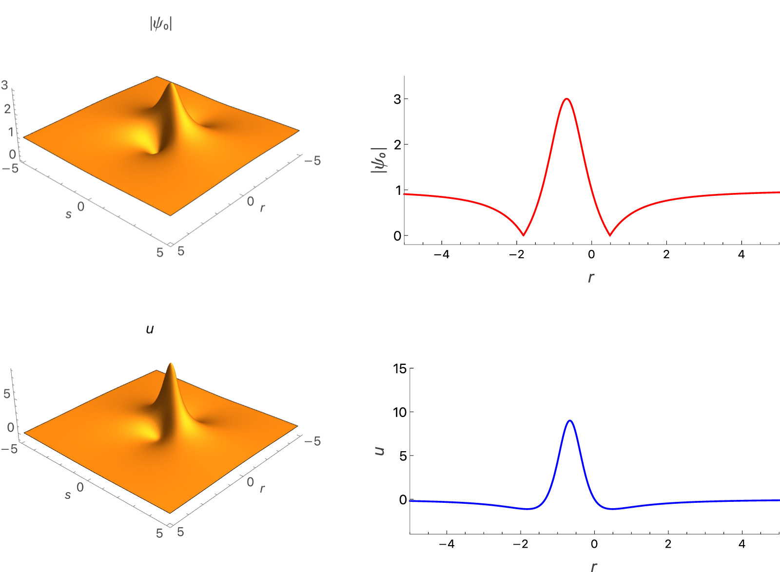


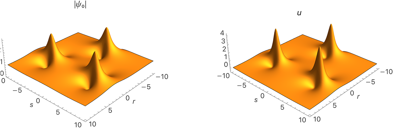


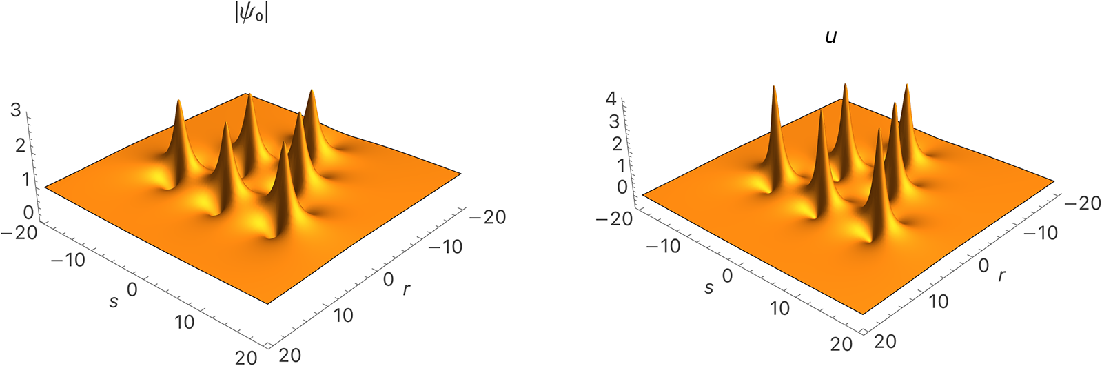


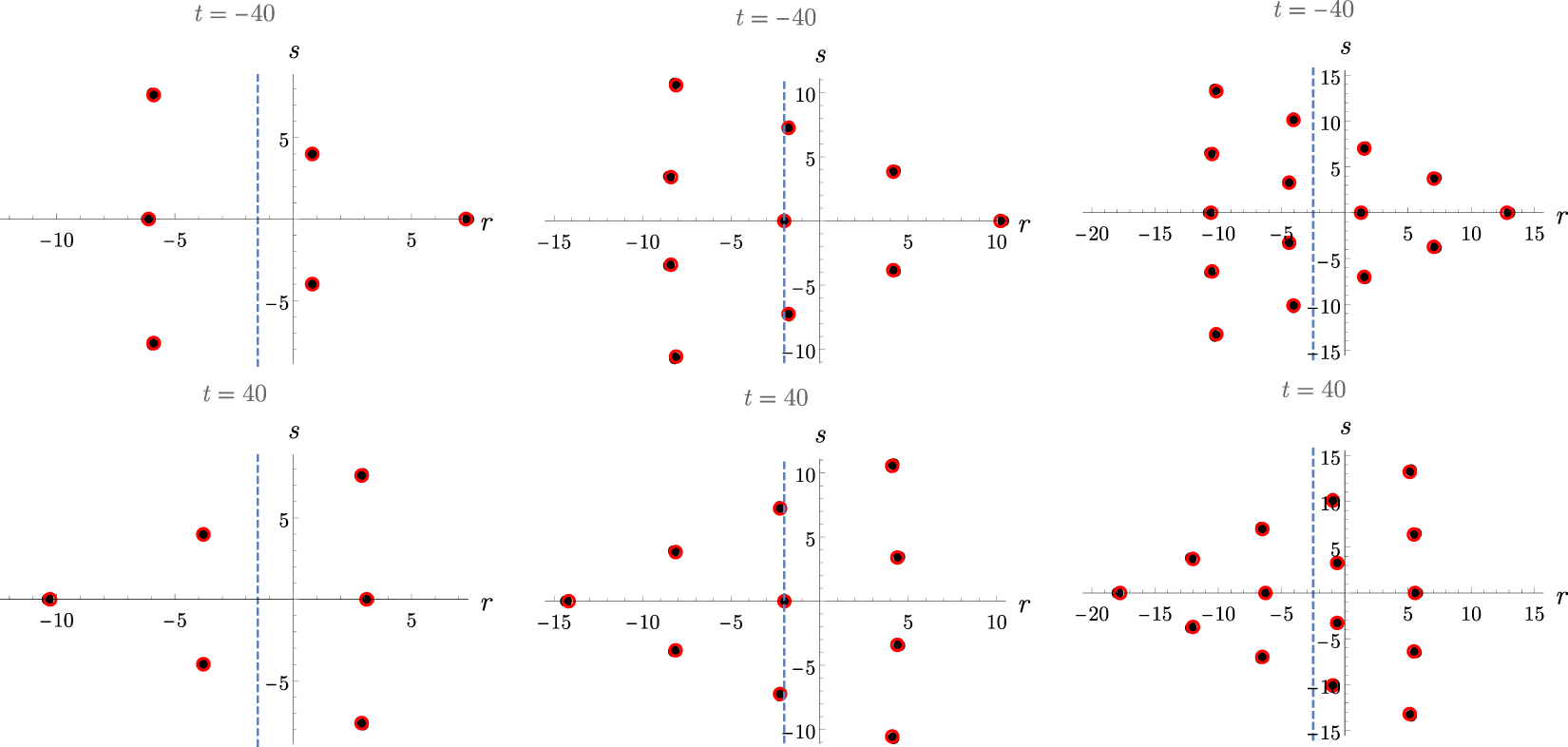


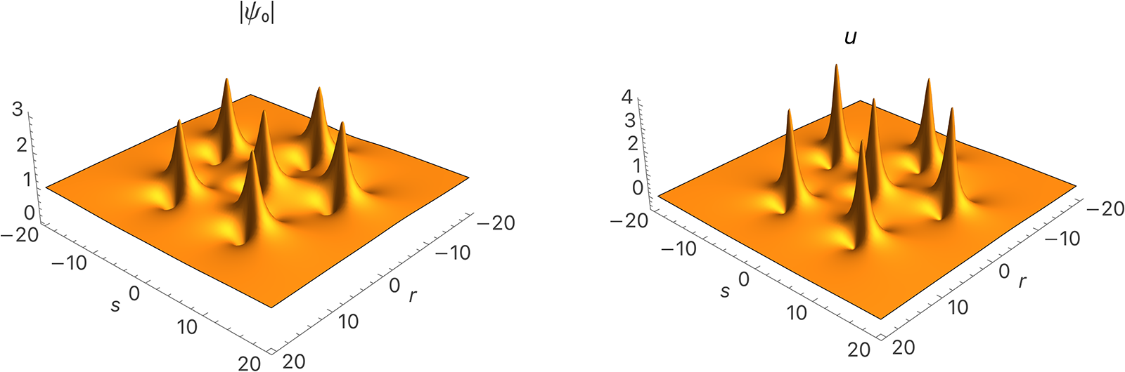


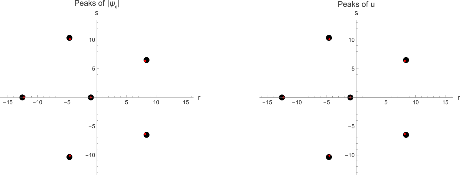


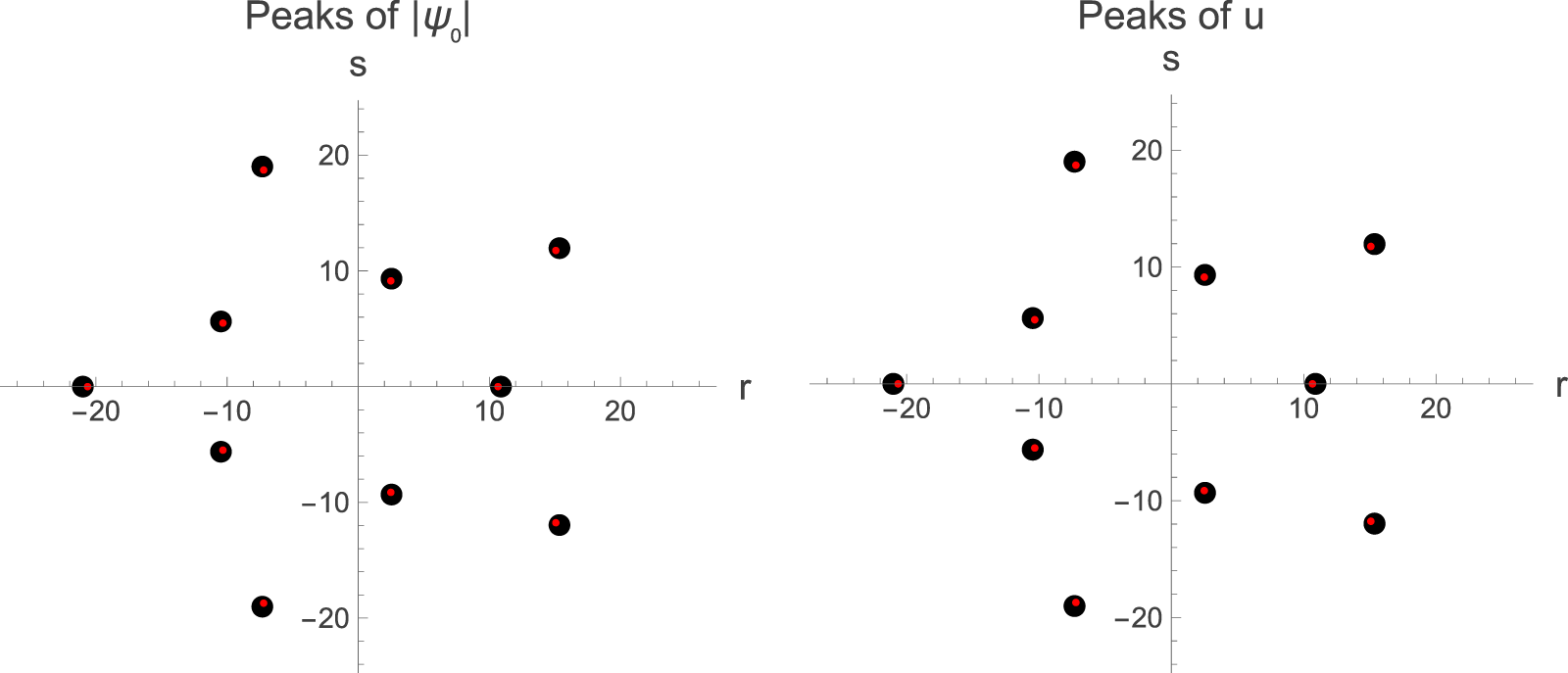


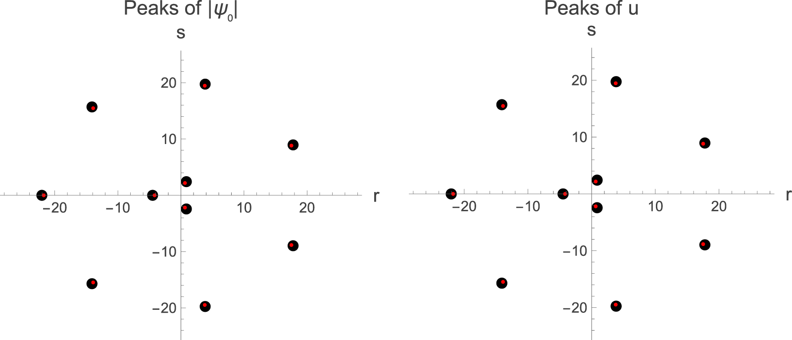


 Open access

