

Introduction
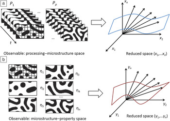
Designing new material and processing protocols requires establishing a relationship between functionality and controllable variables. In principle, materials functionality is associated collectively across length scales with aspects such as chemistry, processing, and microstructure. The relationship across these aspects is established through processing–microstructure–property relationships (PMPRs), which capture two interrelated components—the processing of a material, which results in some microstructure, and the property characterization for a given microstructure. Defining PMPRs is rarely a straightforward task, Reference Rajan1,Reference Ganapathysubramanian and Zabaras2 particularly due to the mismatch between microstructural information that is observed (e.g., via microscopy or simulations) and the principal degree of freedom governing the PMPRs (see Figure 1 ). This is because the goal of microstructural imaging is to provide detailed, high-resolution maps, and hence, imaging techniques inevitably produce high-dimensional data sets, while the goal of establishing quantitative PMPRs is to derive the smallest set of variables that explains most of the variability of the data. However, this set may not be directly measurable or may not be known a priori.
Manifold learning mapping between (left) observable and (right) reduced processing–structure and structure–property spaces. (a) Note the space in which data on processing–microstructure relationships are collected may not be the most robust one. Hence, there is a need to identify the minimal irreducible space where these relationships can be effectively established. Manifold learning techniques can be used to transform the input data into the reduced space. The same argument can be given for (b) the microstructure–property relationship. This approach converts the set of microstructures (discretized into an array of voxels such as shown) into visually interpretable reduced space embeddings (i.e., blue manifold shown for processing–microstructure relationships and red manifold shown for microstructure–property relationships). Adapted with permission from Reference Reference Wodo, Zola, Pokuri, Du and Ganapathysubramanian15. © 2011 Elsevier. Note: P 1,…, P p , p different processing conditions; t, time; x 1,…x n , n different reduced dimensions as a function of processing; η1,… η n , n different properties; y 1,…y n , n different reduced dimensions as a function of property.

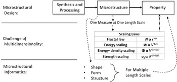
To handle this mismatch challenge, microstructural data sets should be reduced to the meaningful descriptors required to establish PMPRs for the iterative design process of linking theory, modeling, and experiments for improvement and acceleration of materials design. Reference Broderick and Rajan3–Reference Suh and Rajan13 Discovering this reduced descriptor space as applied to microstructure is the basis of microstructural informatics. For example, scaling laws are typically built based on a few microstructural features for defining the localized connection between attribute and property Reference Carpinteri and Pugno14 (see Figure 2 ). Although several scaling laws can be defined over wide ranges of attribute space, no mechanism spanning the scaling laws exists. We discuss an alternative approach based on manifold learning.
Design process for microstructural properties. A synthesis and processing procedure results in some property change due to a change in the microstructure. While multiple characteristics of the microstructure are changing (e.g., shape, form, and structure) at multiple length scales, the high dimensionality typically focuses on correlating one characteristic at one length scale with property (e.g., as is done in scaling laws). The objective of microstructural informatics is to consider the impact on property by the simultaneous role of all characteristics across all length scales, as done with manifold learning mapping (Figure 1). Adapted with permission from Reference Reference Carpinteri and Pugno14. © 2005 Nature Publishing Group. Note: N, number of objects with size larger than r; R, solid size; D, fractal exponent; W, dissipated energy after fragmentation; V, solid volume; Φ, fractal energy density; σc, strength.

In this article, we provide a summary of two independent case studies where microstructural informatics tools uncover structure–processing–property relationships that are otherwise difficult to establish. In the first case study, we discuss how dimensionality-reduction techniques provide insight into the processing–microstructure relationships for the design of organic solar-cell fabrication. In the second case study, we discuss the application of informatics for establishing microstructure–chemistry–property relationships for grain-boundary engineering of metallic systems. In particular, we devise manifold learning techniques (performing a dimensionality reduction analysis by projecting high-dimensional data onto a lower dimensional space while minimizing the loss of information) to build these relationships with the capability of rapidly predicting the properties of new materials, thereby expanding the microstructural knowledge base at a pace not feasible experimentally. We close by discussing the potential benefits that recent high-performance computing (HPC) advances could bring for accelerating the establishment of PMPRs.
Expressing PMPRs in microstructural space
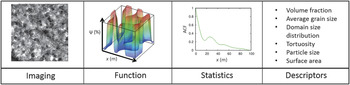
Microstructure constitutes the basis for robust PMPRs, yet no unified definition of microstructure exists. Microstructure can be defined in many different ways. Historically, microstructure was defined by what could be seen under the microscope. Reference Wodo, Zola, Pokuri, Du and Ganapathysubramanian15 Mathematically, microstructure can be seen as the multivariate function or its discrete multidimensional representation, with the multidimensional character of microstructure characterized through imaging, topological functions, or correlative functions, and interpreted by stereology ( Figure 3 ). Moreover, microstructural data sets may be heterogeneous (e.g., real versus spectral, two-dimensional [2D] versus three-dimensional [3D]) and may come from diverse experiments and characterizations focused on specific, potentially incompatible, aspects of microstructure. In such cases, it is necessary to convert heterogeneous microstructural signals into one common space. Stereology is a good example of such a tool, as it focuses on converting the imaged projection of the microstructure in 2D real space with the goal to quantify/deduce 3D space embedding.
Interrogating the multidimensional character of microstructure. Microstructure can be represented as an image, function, statistics, or physically meaningful descriptors. Heterogeneous aspects of the microstructure descriptor significantly contribute to the dimensionality of the data and pose a challenge for manifold learning when establishing processing–microstructure–property relationships. Note: Ψ, volume fraction of a phase (also represented by color mapping); x, distance; ACF, autocorrelation function (unitless).

At the same time, the multidimensional nature of microstructure, coupled with the chemistry of the constituents, offers an almost unlimited phase space and flexibility for the design of materials and processing pathways. However, the large design phase space and corresponding high dimensionality of the microstructural data sets make design a highly challenging problem.
In the context of tackling this dimensionality challenge, we suggest employing manifold learning, a powerful mathematical tool that projects high-dimensional data onto a principal manifold while preserving the characteristic properties. In this way, large microstructural data sets can be rigorously compacted to effectively express the interplay between processing, chemistry, morphology, and properties. Projecting data onto a lower dimensional space (1) compresses the data and allows for deriving the key features governing the PMPRs; (2) enables visualization of the high-dimensional space; and (3) unravels the dominant structure hidden in the data regardless of the noise potentially present in the data.
Uncovering processing–chemistry–microstructure–property relationships using microstructural informatics
Case study 1: Data-driven morphology annotation to design the optimal fabrication pathway for organic solar cells
Organic solar cells have the potential to revolutionize the portable electronics market due to their unique properties, including transparency, ability to bend, stretch, and conform to various geometries, and, above all, their low weight. However, mass production is still bottlenecked due to their relatively low efficiency and short life spans. Improvements in efficiencies have come from optimizing material processing in order to alter the microstructure, as the efficiency is a strong function of the microstructure.
For example, we consider microstructural evolution during the manufacturing of organic thin films Reference Wodo and Ganapathysubramanian16,Reference Wodo and Ganapathysubramanian17 with substrate patterning, described by patterning frequency (l p) and intensity (μ). Substrate patterning is an effective way to manipulate the thin-film morphology into an arbitrary structure, potentially allowing us to obtain the desired properties. The overarching goal is to rationally tailor processing pathways and identify the optimal processing conditions to fabricate films with the desired internal structure. The objective of this study Reference Wodo and Ganapathysubramanian16,Reference Wodo and Ganapathysubramanian17 was to (1) screen two process variables (l p and μ); (2) collect the evolution of microstructure for each variant of processing; and (3) retransform the microstructural data into a manageable yet meaningful space to facilitate the optimization of manufacturing.
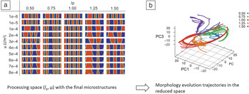
The high-throughput exploration of various manufacturing parameters was performed using phase-field modeling for morphology evolution during thermal annealing of the organic thin films. Reference Wodo and Ganapathysubramanian16–Reference Sumudrala, Zola, Aluru and Ganapathysubramanian18 For each manufacturing variant, the temporal evolution of microstructure was stored. Collectively, 75,150 representative microstructures were stored for the analysis. Each microstructure was represented as an image converted into an 8326-dimensional array of pixel composition values. Figure 4a depicts examples of the final microstructure for the processing variants. Note the size of the data inhibits any realistic reasoning of the data and motivates the usage of the manifold learning technique.
(a) The final microstructures corresponding to two process variables—pattern frequency and patterning intensity in the processing of organic thin films and the change in the microstructure as a function of patterning organic thin films for photovoltaic processing (the colors reflect the volume fraction of the polymeric phases). (b) Microstructure evolution trajectories corresponding to 50 different manufacturing processes captured by the first three principal components (PC1, PC2, PC3) of the original data (colors as denoted by the key correspond to l p). Each point corresponds to one microstructure. Note that transforming the original data into the reduced space reveals multiple highly similar fabrication routes, and multiple diverse routes that lead to a similar intermediate or final microstructure. Adapted with permission from Reference Reference Sumudrala, Zola, Aluru and Ganapathysubramanian18. © 2016 Elsevier. Note: μ, chemical potential (J/m3); l p, frequency of patterning (unitless).

To tackle the large data sets, spectral dimensionality reduction techniques Reference Sumudrala, Zola, Aluru and Ganapathysubramanian18 have been applied. In general, these techniques produce a mapping function that transforms the high-dimensional input data into low-dimensional embedding, while preserving the characteristic property. Figure 4b plots all of the microstructures in a reduced 3D space, where each point corresponds to one microstructure. In this case, the reduced space is constructed with only the first three principal components of the data, which capture ∼70% of the information content of the entire data. Note the original dimensionality of the problem was 8326 (size of an individual microstructure). The dimensionality of the reduced space constitutes 0.03% of the dimensionality of the original space (three dimensions out of the original 8326). This emphasizes the power of this approach for extracting meaningful conclusions rapidly while preserving crucial information.
Transforming the original data into the reduced space effectively brings the original data into a more visually intuitive space and makes quantitative and qualitative analysis possible. In this case study, the effects of processing on the microstructure could be investigated. In particular, the following questions, otherwise intractable to even approach, can be answered:
-
1. What is the simplest route to manufacture a desired microstructure?
In Figure 4, multiple microstructural trajectories are plotted in the reduced space, with several pathways reaching a similar final structure. By identifying the shortest pathway to reach the desired microstructure, the most optimal manufacturing process can be extracted. This is based on the assumption that the shortest pathway corresponds to the simplest morphology evolution pattern, regardless of the physical interpretation (or lack of physical interpretation) of the reduced order space.
-
2. What is the optimal processing range?
From Figure 4, the microstructure evolution trajectories can be inspected to first, identify highly similar or overlapping pathways, and next, compare the corresponding range of processing conditions. This question is of particular importance when manufacturing is highly sensitive to small modifications in processing conditions.
-
3. Can a desired microstructure be obtained using fewer processing steps?
Analysis of the evolution trajectories provides insight into this optimization problem. Specifically, simultaneously embedding multiple trajectories in the common low-dimensional space allows us to seek potential intersections between variants of fabrication. The intersection can be seen as the transfer point between the processing steps in the hybrid processing. Similar microstructures have the same coordinates in the common reduced space. The intersection between different trajectories indicates when transferring between the two processing conditions is feasible.
Case study 2: Informatics for building property libraries of grain boundaries
Grain-boundary engineering seeks the connection between the crystallography of grain boundaries and the physical properties of materials. Examples within this objective include stress-corrosion cracking, Reference Frankel19,Reference Burleigh20 grain-boundary embrittlement, Reference Cantwell, Tang, Dillon, Luo, Rohrer and Harmer21 and creep, Reference Yamakov, Wolf, Phillpot and Gleiter22,Reference Markmann, Bunzel, Rosner, Liu, Padmanabhan, Birringer, Gleiter and Weissmuller23 among others. The objective of microstructural informatics is to derive grain-boundary–chemistry–property relationships and, subsequently, use these to construct larger libraries. Adding information on the grain boundary fills the gap in the relationship between processing and property.
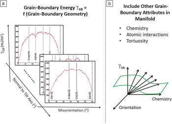
Results were taken from grain-boundary energy calculations Reference Tschopp, Solanki, Gao, Sun, Khaleel and Horstemeyer24 and supplemented with additional microstructural data on other elements, the corresponding interactions, and any other potentially relevant descriptors. The logic utilized has been described and successfully applied to multiple material and data spaces, Reference Broderick, Bryden, Suram and Rajan25–Reference Broderick and Rajan31 leading to expanded materials libraries. The challenge, and the motivation for applying microstructural informatics, is to extract the relationships between microstructure and properties that can be used in the design of new materials (see Figure 5 ). In general, we build relationships based on descriptors that are either known in all cases, or else can be easily measured. In this case, the grain-boundary energy calculated for all orientations and chemistries would be the preferred data. However, obtaining this information is highly challenging.
Role of informatics for describing grain-boundary energetics as a function of multiple attributes and not just as a function of a single attribute (i.e., geometry). (a) Each point in the energy landscape contributes a point on the property plane (orientation–energy). The vertical lines indicate grain boundaries with a low degree of fit (Σ). (b) When we integrate other attributes with this plane, this point instead is projected onto the reduced-space manifold. Adapted with permission from Reference Reference Tschopp, Solanki, Gao, Sun, Khaleel and Horstemeyer24. © 2012 IOP Publishing.

To bypass this challenge, we seek the minimal combinations of descriptors that serve as a surrogate for the grain-boundary energy. The database used in this case study has 34 chemical descriptors and six microstructural properties, thereby representing a 40-dimensional space. Within this space and given the existing intercorrelations, we employ manifold mapping to identify the key descriptors for the surrogate model. This step requires a converted mapping of not only the chemistries, but, more importantly, the descriptors in an interpretable form. While we have also used nonlinear manifold mappings Reference Srinivasan, Broderick, Zhang, Mishra, Sinnott, Saxena, LeBeau and Rajan32 that may more accurately capture the manifold topology, these do not provide a measure of descriptor correlation.
As an example, using principal component analysis (PCA), we analyzed the (21 × 40) data matrix X with a manifold learning approach, where we transform X into a matrix correlating the control combinations (T) and the descriptors (P X) and properties (P p). PCA is a mathematical tool that transforms the original descriptor space into a reduced space where the axes of a reduced space are defined by a linear combination of the original descriptors. These new axes (principal components) capture independent information and therefore, allow us to extract the underlying relationships that are potentially hidden in the large and intercorrelated input descriptor space. PCA also inherently ranks the amount of variance in the original data captured by each principal component, and in this way, leads to reduced dimensionality with minimal information loss by screening out those principal components that capture primarily uncertainty, error, or noise. The proximity and trajectory of points within the principal component space allow us to calculate correlation and, for a correlation cutoff, identify the relevant descriptors for property prediction. A multiple linear regression is then performed between the reduced descriptor space and the reduced property space. The output of our model is then of the form:
 $${{\bf{\gamma }}_i = \mathop \sum \limits_{j = PCs} \beta _j T_{i,j} + C,$$
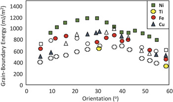
where γ is the grain-boundary energy, T is the output from the PCA analysis (i.e., a linear combination of descriptors related to the chemistry and includes radii, electronegativity, and properties of the single-phase elements), and β and C are a function of both misorientation angle and chemistry. The number of principal components refers to the dimensionality used in the reduced manifold space (j in the equation), while i refers to the unique set of conditions of misorientation and chemistry that are being predicted. This provides regression terms in a common format with material condition terms (i.e., the original data projected onto the transposed axis space), and represents an alternative representation (quantitative structure–property relationship—QSPR) of the microstructure. This QSPR allows us to develop libraries of microstructural properties (see Figure 6 ) Reference Bulatov, Reed and Kumar33,Reference Ratanaphan, Olmsted, Bulatov, Holm, Rollett and Rohrer34 as the required model inputs are known for nearly all elements. From the QSPR, we can rapidly calculate properties for a larger number of materials than is possible through electronic structure calculations or experiments, which require either knowledge of input potentials or are time-consuming. That is, we use a relationship for which the required inputs are either known or may be calculated even for unexplored materials.
Development of grain-boundary property libraries. The open symbol shapes represent training data, while the closed shapes are those predicted by the model, following the predictive approach described in Reference Reference Andriotis, Mpourmpakis, Broderick, Rajan, Datta, Sunkara and Menon30. While this can be theoretically expanded to any combination of chemistry and orientation, we limit this here to only chemistries and orientations contained in training data to minimize uncertainty. This demonstrates the capability to rapidly model properties of grain boundaries and not just the properties of materials. Adapted with permission from Reference Reference Tschopp, Solanki, Gao, Sun, Khaleel and Horstemeyer24. © 2012 IOP Publishing; Reference Reference Bulatov, Reed and Kumar33. © 2014 Elsevier; and Reference Reference Ratanaphan, Olmsted, Bulatov, Holm, Rollett and Rohrer34. © 2014 Elsevier.

From a small number of training points, we can thus expand the knowledge space to a far greater number. This then provides guidelines for identifying a few additional calculations or experiments that are needed—whether to test a condition predicted as having unique properties, or else to introduce additional physics into the training data, such as expanding from single-element systems to alloy systems. Establishing microstructure–property models by harnessing manifold learning accelerates the discovery process by both guiding the necessary empirical measurements while simultaneously reducing the number of measurements required.
A couple of comments should be made here on accounting for uncertainty, which is present at every stage—in the training data from computation/experiment, in the selection of descriptors for the surrogate model, and in the prediction of property values. While we do not explicitly quantify uncertainty here, our model is built with the consideration of the tradeoff between robustness and accuracy, thereby attempting to maintain consistent levels of uncertainty across the entire process. That is, through the cross-validation process (i.e., training the model on some of the data and testing the model on other data), we identify what provides the best tradeoff by roughly equating the training and testing accuracies. This type of model has the benefit of being computationally tractable and is based primarily on existing knowledge in databases.
Need for harnessing HPC to establish PMPRs
Establishing reliable PMPRs depends on the size of the explored phase space of processing conditions and the chemistries and materials screened. Even the simplest manufacturing process involves multiple processing parameters that should be sampled with high frequency. This number increases even more for complex multistage processing. Thus, the “phase space” over which the exploration has to be performed induces the “combinatorial explosion” of possibilities for the analysis.
Such large-scale exploration can rarely be performed manually, but rather necessitates an automated, high-throughput exploration. In the case of experimental exploration, the automation can be facilitated by robotics and data processing in order to conduct millions of tests. In the case of computational exploration, automation can be achieved with HPC tools combined with data analytics tools. However, devising such a workflow requires substantial domain expertise in software engineering, fault tolerant computing, and HPC in general. This may hamper a materials science domain expert from performing large-scale PMPR studies without investing substantial resources and effort in acquiring the required HPC expertise.
We advocate the use of cloud computing—the increasingly popular technology where sharing large data and performing large-scale computation is almost transparent to the user. In cloud computing, the user does not know where the data is stored or processed. Moreover, the computations can scale up or down depending on the current needs. The only requirement to execute the computation in the cloud is to express the workflow using a specific protocol; the MapReduce programming pattern is an example of such a protocol. Reference Wodo, Zola, Pokuri, Du and Ganapathysubramanian15 Google has introduced this pattern to unify large-scale computing and hide low-level computing details from the user. Generally speaking, the MapReduce protocol relies on two basic operations—mapping and reducing. As long as the specific problem can be expressed using these two operations, the computations can be seamlessly orchestrated by a nonexpert. We argue that the MapReduce paradigm is ideally suited to execute processing–microstructure–property exploration.
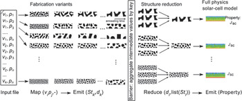
Consider a problem of linking processing → structure for a given set of processing conditions and the corresponding microstructure(s). Using the MapReduce protocol, this task can be simply formulated as a function that maps processing variables with the corresponding microstructure. MapReduce can independently orchestrate multiple processing variants on the currently available resources in the cloud environment. Each execution generates the corresponding microstructures that can be annotated with the descriptors. In particular, MapReduce outputs physically meaningful descriptors (e.g., grain-size distribution, orientation distribution, and interfacial area) that later on are used in the reducing function. The key idea is that all computations can be fully automated in a fault-tolerant fashion.
Now consider a second step of linking structure → property for given characterized properties from various microstructure classes. Note that homologous microstructures (i.e., microstructures with the same descriptor) will be statistically characterized by the same properties ( Figure 7 ). Hence, we can organize all microstructures into a set of equivalent property classes and then identify properties on a per-class basis. MapReduce can internally organize microstructures into classes in terms of storage and communication between potentially distant locations where computations were executed. The user only needs to specify the reduction criteria. This conceptual step can be again automated with minimal input from the materials science expert.
Linking process–structure–property and expressing it using the MapReduce paradigm. High-throughput exploration of process–microstructure–property space can be naturally expressed as a two-step process in MapReduce. This enables large-space execution in the cloud environment through map, reduce, and emit functions, requiring minimal expertise in high-performance computing on the part of the materials researcher. Reprinted with permission from Reference Reference Wodo, Zola, Pokuri, Du and Ganapathysubramanian15. © 2011 Elsevier. Note: v 1, p 1….v i , p j , different processing system variables; St k , microstructures; d k , descriptors; d l , subset of descriptors; St l , subset of microstructures sharing the same d l ; J sc, short-circuit current.

The logic of PMPRs is highly consistent with the two-step MapReduce paradigm. The cloud infrastructure can be deployed to automatically execute the complex combinatorial task of running tens or even hundreds of thousands of process → structure and structure → property (PSP) evaluations. Figure 7 illustrates the PSP linkage expressed using the MapReduce paradigm. We performed analysis involving the exploration of 100 manufacturing variants of organic thin films, with 32,000 microstructures generated. In the reduction step, 2000 microstructures were characterized using a full physics solar-cell simulator to compute the short-circuit current. The total execution time was ∼48 hours on the 32-node cluster. Reference Wodo, Zola, Pokuri, Du and Ganapathysubramanian15 We specifically established correlations between microstructure and efficiency of the photovoltaic process. Through the high-throughput analysis, we found three morphological traits that correlate well with the short-circuit current. Since the short-circuit current directly translates to the solar-cell efficiency, finding morphology with high current has significant implications for the design of morphologies for high-performance organic photovoltaic devices.
Summary
In this article, for a given class of microstructure, we discussed (1) a reduced representation of microstructure for defining similarities based on various processing conditions; (2) relationships between microstructure and property; and (3) chemistry–property relationships. The construction of reliable PMPRs is a challenging process. The associated challenges include the collection and handling of multidimensional data sets from experiments and computational studies; the quantitative analysis of data in a statistically robust yet physically meaningful manner; and the building of the manifold representation of PMPRs that both explain known materials behavior and guide the pathways for designing new materials with enhanced properties. We have given special attention to the predictive capabilities of PMPRs for catalyzing new design routes for the accelerated discovery of PMPRs. These integrated approaches contribute to the building of massive “virtual” material databases that may enhance the future design of materials and processing, and may be mined in the future to identify the processing conditions that lead to the combination of desired responses.
Acknowledgments
S.B. and K.R. acknowledge support from the Air Force Office of Scientific Research, under Grant Numbers FA9550–12–1-046 and FA9550–11–1-0158, and the National Science Foundation, under Grant Number DMR-13–07811. K.R. also acknowledges the Erich Bloch Endowed Chair at the University at Buffalo, The State University of New York.