


1. Introduction
A stable demand function for money is crucial for ensuring that money exerts a predictable influence on the economy, thereby enabling the money supply to function as an effective tool for economic policy (Serletis, Reference Serletis2007). Consequently, identifying potential distortions in the money demand function has been a subject of extensive debate and research among economists and academics (for surveys, see Sriram, Reference Sriram2000; Knell and Stix, Reference Knell and Stix2006). Properly identifying structural breaks in the money demand function, as an indicator of instability, is consistently accompanied by technical challenges. Notably, despite extensive research, there remains no consensus on the appropriate functional form for incorporating monetary aggregates and their user costs into the money demand function (Watanabe and Yabu, Reference Watanabe and Yabu2023). Due to these challenges, scholars turn to flexible diagnostic tools to unravel the potential money demand instabilities (e.g., Bissoondeeal et al., Reference Bissoondeeal, Binner and Karoglou2023; Dai and Serletis, Reference Dai and Serletis2019; Movaghari et al., Reference Movaghari, Serletis and Sermpinis2024).
In this study, we employ the copula technique to revisit the stability of money demand by investigating potential changes in the dependence structure between broad monetary aggregates (Sum M2, Divisia M2, and Divisia M4) and their user costs. A copula is a function that joins a multivariate distribution function to their one-dimensional marginal distribution functions (Nelson, Reference Nelsen2006). In other words, a copula “couples” marginal distributions into a joint distribution (Xiong and Cribben, Reference Xiong and Cribben2023).
Traditionally, a stable demand for money function implies that money holdings can be explained, with conventionally acceptable statistical significance, by a stable functional relationship involving a relatively small number of determinants, such as income, user cost, and expected inflation (Laidler, Reference Laidler1982; Barnett et al., Reference Barnett, Ghosh and Adil2022). In the conventional literature, stability is therefore commonly associated with parameter constancy, cointegration stability, and forecasting performance.Footnote 1 By contrast, this paper focuses on the stability of the dependence structure between money demand and user cost, as captured by copula models. Under the assumptions of linearity and normality, the regression coefficient in a simple model with one regressor has a direct relationship with the Gaussian copula parameter. Consequently, instability in regression coefficients would generally be reflected in the copula dependence parameter. However, this relationship is not always straightforward, particularly because the assumptions of linearity and normality have recently been questioned in literature (e.g., Benati et al., Reference Benati, Lucas, Nicolini and Weber2021; Gao et al., Reference Gao, Whited and Zhang2021). Copula methods provide a more flexible framework capable of capturing nonlinear, asymmetric, and tail-dependent relationships that conventional linear specifications may fail to detect. Therefore, instability in the copula dependence structure should be viewed as a broader concept than conventional regression instability.
Using copula method to find structural breaks in the money demand function has two main advantages. First, a copula function can effectively capture the overall dependence between variables (Zhu et al., Reference Zhu, Xie, Li and Wu2015). Considering recent evidence of nonlinear relationship between interest rates and money demand (Gao et al., Reference Gao, Whited and Zhang2021), incorporating nonlinearity is crucial for examining money demand stability. In addition, Benati et al. (Reference Benati, Lucas, Nicolini and Weber2021) document that the empirical money demand curve does not follow the theoretical model in the region of very low interest rates, highlighting the necessity of considering tail dependencies in developing money demand function. The capabilities of copula technique enables us to transcend the limitations of linear correlation when analyzing the relationship between money supply and user cost. Second, it relaxes the need to precisely specify the functional form of the money demand function, such as log–log, semi-log, or Selden-Latané specifications (Cagan, Reference Cagan1954; Latané, Reference Latané1960; Meltzer, Reference Meltzer1963; Selden, Reference Selden1956), thereby offering greater flexibility in modeling potentially complex relationships between the two components. The sole prerequisite to employ copula function is that the original variables must be distributed within the unit interval (0, 1). In practice, this condition is readily satisfied by pseudo-observations generated from the given data matrix.Footnote 2
To identify changepoints in the money demand function, we follow Zhu et al. (Reference Zhu, Xie, Li and Wu2015) and employ a rolling time-varying approach. Particularly, we first find the best copula family for the entire period. Then, we estimate the identified copula family over rolling windows to establish a one-dimensional time series of copula parameters. The copula parameters are estimated using the maximum pseudo-likelihood method. Finally, we conduct Bai and Perron’s (Reference Bai and Perron2003) test to identify potential structural break(s) in the univariate time series of copula parameters. In our analysis, four common copula families are considered: Student-t, Gaussian, Frank, and Clayton, following Following Ruppert and Matteson (Reference Ruppert and Matteson2011).
Analyzing quarterly data from Federal Reserve Economic Data (FRED) for the period 1967:Q1–2025:Q1, we observe that Gaussian copula family are best suited for modeling the dependence structure of money demand function based on traditional simple-sum measures. We identify two changepoints in the dependence structure between Sum M2 and its user cost, mirrored in the univariate time series of Gaussian copula parameters. Changepoints are identified at 1983:Q4 and 2001:Q4. The identification of these breakpoints is robust to alternative choices of window length in the rolling time-varying estimation approach. They are also supported by the pattern of changes in the cumulative sum (CUSUM) prosses of Ploberger and Krämer (Reference Ploberger and Krämer1992).
The two changepoints in the dependence structure of simple-sum measures are closely align with the widely recognized beginning and end of the Great Moderation period (e.g., Belongia and Ireland, Reference Belongia and Ireland2016; Guerron-Quintana, Reference Guerron-Quintana2009). The onset of the Great Moderation followed a significant wave of U.S. financial deregulation in the 1980s, including the gradual removal of interest rate ceilings under Regulation Q (Koch, Reference Koch2015), as well as improvements in monetary policy and other structural factors. Lucas and Nicolini (Reference Lucas and Nicolini2015) identify the gradual removal of Regulation Q as a key factor contributing to money demand instability in the 1980s. The Great Moderation period persisted until the early 2000s, when the Federal Reserve appears to have shifted its policy focus from strict inflation control, characteristic of the 1980s and 1990s, toward a greater emphasis on smoothing real economic fluctuations (Belongia and Ireland, Reference Belongia and Ireland2016; Lubik and Schorfheide, Reference Lubik and Schorfheide2004).
Turning to the Divisia measures provided by the Center for Financial Stability (CFS), we find that the Clayton copula family performs best in capturing the dependence structure between Divisia measures (M2 and M4) and their user costs. We identify three changepoints for Divisia M2, occurring at 1986:Q2, 1994:Q2, and 2017:Q4. Similarly, for Divisia M4, we identify three changepoints at 1986:Q4, 1994:Q3, and 2013:Q1. The first changepoint coincides with the initial shift observed in the dependence structure of simple-sum measures, confirming the instability of Divisia measures following the banking deregulation of the 1980s (e.g., Bordo and Duca, Reference Bordo and Duca2025; Spencer, Reference Spencer1988). In contrast to traditional measures, our results also indicate the presence of a changepoint in the dependence structure of Divisia measures in the mid-1990s, potentially reflecting the impact of significant financial innovations during that decade, particularly the introduction of sweep technology (Teles and Zhou, Reference Teles and Zhou2005). Berentsen et al. (Reference Berentsen, Huber and Marchesiani2015) provide evidence that sweep technology contributed to the observed patterns in money demand during the 1990s. To empirically assess this conjecture, we examine the stability properties of the copula parameters for the Monetary Services Index (MSI) M2 developed by Anderson and Jones (Reference Anderson and Jones2011), which is hypothesized to absorb the effects of retail sweep programs on Divisia M2. Our results indicate that the half-life measure of the copula dependence parameter for MSI M2 is indeed approximately one and a half times shorter than that of Divisia M2. Interestingly, the selected copula family for MSI M2 is the Frank copula, which, like the copulas selected for Divisia M2 and Divisia M4, belongs to the Archimedean class of copulas.
Given the fewer breakpoints in the simple-sum-based copula parameters compared to the Divisia-based parameters (two versus three), one might argue that the simple-sum measure could be a more suitable candidate for studying the money demand function. However, an examination of the autocorrelation function (ACF) of the copula parameters indicates that there is no substantial difference between simple-sum and Divisia measures in terms of the stability of the money demand dependence structure. In addition, we find that the half-life estimates and unit root test statistics for the Divisia measures are smaller than those of the simple-sum measure. These mixed empirical results challenge the notion, often suggested in the literature, that Divisia measures are superior for analyzing the effectiveness of monetary policy (e.g., Jadidzadeh and Serletis, Reference Jadidzadeh and Serletis2019; Lucas, Reference Lucas2000).
Our results are robust to alternative window lengths in the rolling time-varying approach. Furthermore, we document that macroeconomic indicators such as the zero lower bound, high inflation periods, and recessions do not have statistically significant effects on the time series of the copula parameter for both simple-sum and Divisia measures. This suggests that the detected shifts in dependence are unlikely to be driven solely by broader macroeconomic conditions.
This study makes three key contributions. First, it expands the existing literature on money demand stability by incorporating the copula approach. Amid the ongoing debate on the functional form of the money demand function (e.g., Ireland, Reference Ireland2009; Lucas, Reference Lucas2000; Lucas and Nicolini, Reference Lucas and Nicolini2015), the copula technique mitigates the need for explicitly specifying the functional relationship between monetary aggregates and user costs. By using the copula approach, we are able to capture various dependence structures, including nonlinearity and tail dependencies (Li and Li, Reference Li and Li2015; Liu and Serletis, Reference Liu and Serletis2022).
Second, while our results continue to confirm the potential influence of financial deregulation and innovation in the 1980s and 1990s, respectively, on money demand, they also emphasize the need for further research on monetary policies in the 2000s and 2010s. In particular, we find evidence of changepoints in the dependence patterns of the simple-sum and Divisia measures, occurring in the early 2000s and 2010s, respectively. According to existing literature, there is a paucity of studies analyzing monetary policies in recent decades (e.g., Belongia and Ireland, Reference Belongia and Ireland2016; Clarida, Reference Clarida2012; Wang, Reference Wang2024).
Finally, our study joins the mainstream of literature that leverages the strengths of copulas to examine empirical relationships between variables in economics and finance (e.g., Collins and Gallagher, Reference Collins and Gallagher2016; Huang et al., Reference Huang, Mollick and Nguyen2017; Li and Li, Reference Li and Li2015; Liu and Serletis, Reference Liu and Serletis2022; Wang et al., Reference Wang, Wu and Lai2013; Ye et al., Reference Ye, Liu and Miao2012; Zhu et al., Reference Zhu, Xie, Li and Wu2015). Particularly, we can find several studies in monetary economics that utilize copula technique to analyze the connectedness between monetary aggregate and platinum-group elements (Fernandez, Reference Fernandez2017), commodity prices, the US interest rate, and the US dollar (Huang et al., Reference Huang, Mollick and Nguyen2017), credit card transaction services and the monetary assets (Liu and Serletis, Reference Liu and Serletis2022), money and the level of economic activity (Serletis and Xu, Reference Serletis and Xu2022), among others.
The rest of the paper is organized as follows. Section 2 explains the copula method and how we employ this technique to determine breakpoint(s) in the money demand function. Section 3 describes the time series data. Section 4 present the results. Section 5 concludes the paper.
2. Methodology
2.1. Dependence structure and copulas
A copula is a multivariate cumulative distribution function (CDF), and its univariate margins is uniform over the unit interval (0, 1) (Wang et al., Reference Wang, Wu and Lai2013; Xiong and Cribben, Reference Xiong and Cribben2023). More specifically, let
 $Y=(Y_1,\ldots ,Y_d)$
is a d-dimensional vector of random variables. Denote the marginal univariate CDFs of
 $Y_1,\ldots ,Y_d$
by
 $F_{Y1}(y_1),\ldots ,F_{Y_d}(y_d)$
, respecively. Then, the multivariate CDF of {
 $F_{Y1}(y_1),\ldots ,F_{Y_d}(y_d)$
} is a copula. This CDF is called the copula of
 $Y$
and denoted by
 $C_Y$
(Ruppert and Matteson, Reference Ruppert and Matteson2011). According to Sklar’s (Reference Sklar1959) theorem, assuming that
 $F_{Y_j}$
s (
 $j=1,\ldots ,d$
) are continuous, every continuous cdf
 $F_Y$
has a unique copula
 $C_Y$
that satisfies:
 \begin{equation} F_Y (y_1,\ldots ,y_d) = C_Y\{F_{Y_1}(y_1),\ldots ,F_{Y_d}(y_d)\} . \end{equation}
The Sklar’s theorem states that a joint CDF
 $F_Y$
can be decomposed into marginal CDFs
 $F_{Y_1}(y_1),\ldots ,F_{Y_d}(y_d)$
, which contain all information about the univariate marginal distributions, and a copula
 $C_Y$
, which contains all information about the dependencies among
 $Y_1,\ldots ,Y_d$
(Ruppert and Matteson, Reference Ruppert and Matteson2011).
Several types of copula families (or classes) are commonly used in the literature, including Gaussian (normal), Student-t, Clayton, and Frank. The first two belong to the elliptical copula family, while the latter two fall under the Archimedean copula category (e.g., Nelsen, Reference Nelsen2006; Ruppert and Matteson, Reference Ruppert and Matteson2011).
Suppose
 $u_1$
and
 $u_2$
are two random variables uniformly distributed in the unit interval
 $[0, 1]$
. The Gaussian copula for
 $u_1$
and
 $u_2$
is given by (Kole et al., Reference Kole, Koedijk and Verbeek2007; Ruppert and Matteson, Reference Ruppert and Matteson2011):
 \begin{align} C_{Gauss}(u_1,u_2|\rho ) = \Phi (\Phi ^{-1}(u_1), \Phi ^{-1}(u_2)|\rho ) \hspace {1cm} \end{align}
where
 $\Phi$
and
 $\Phi ^{-1}$
are the CDF of the standard bivariate normal distribution and the corresponding inverse CDF of the standard normal distribution, respectively. In Gaussian copula there is only one parameter, i.e.,
 $\rho$
, which measures the correlation between two random variables. Similarly, the Student-t copula is defined by (Ruppert and Matteson, Reference Ruppert and Matteson2011):
 \begin{align} C_{t}(u_1,u_2|\rho ,\nu ) = \Psi (\Psi ^{-1}(u_1), \Psi ^{-1}(u_2)|\rho ,\nu ) \end{align}
where
 $\Psi$
and
 $\Psi ^{-1}$
are the CDF of the bivariate Student-t distribution and the inverse of the CDF for the univariate Student-t distribution, respectively. Unlike Gaussian copula, Student-t copula is characterized by two parameters:
 $\nu$
the degrees of freedom parameter and
 $\rho$
the correlation parameter.
Next, we introduce the two members of the Achimedean copula family. The bivariate Frank family is defined by the following function (Nelsen, Reference Nelsen2006):
 \begin{align} C_{Fr}(u_1,u_2|\theta ) &= -\frac {1}{\theta }\ln \Big ( 1+\frac {(e^{-\theta u_1 }-1)(e^{-\theta u_2 }-1)}{e^{-\theta }-1} \Big ) \end{align}
where
 $\theta$
is the dependence parameter which takes values in
 $({-}\infty ,\infty )-\{0\}$
. For Frank copula,
 $\theta \rightarrow 0$
is an indication of independence structure between two variables (Ruppert and Matteson, Reference Ruppert and Matteson2011). The Clayton family is defined by the following function (Nelsen, Reference Nelsen2006):
 \begin{align} C_{Cl}(u_1,u_2|\theta )&=\big [{\max}\big \{u_1^{-\theta }+u_2^{-\theta }-1,0\big \}\big ]^{-\frac {1}{\theta }} \end{align}
where
 $\theta$
is the dependence parameter, ranging from –1 to
 $\infty$
, excluding zero. One advantage of the Archimedean copula family over the elliptical family is their simplicity in terms of mathematical formulation and expression (Ye et al., Reference Ye, Liu and Miao2012). Elliptical copulas are characterized by integrals, whereas Archimedean copulas possess explicit closed-form expressions, as evident from Equations (2)–(5). Another benefit of Archimedean copulas over elliptical copulas is their simpler parametrization. Frank and Clayton copulas are characterized by only one parameter, compared to the Student-t copula which has two parameters, which makes estimation quite straightforward. For a detailed description of copula families, we refer to Cherubini et al. (Reference Cherubini, Luciano and Vecchiato2004, Chapter 3) and Nelsen (Reference Nelsen2006, Chapter 4).
2.2. Copula-based changepoint analysis
In this paper, we leverage copula capabilities to detect potential instabilities in the dependence structure of money demand equation. To this end, we apply the three-step method of Zhu et al. (Reference Zhu, Xie, Li and Wu2015):Footnote 3
-
• Step 1: Identify the best copula to capture the dependence structure between monetary aggregates and their user costs.
-
• Step 2: Estimate the copula parameter over rolling windows.
-
• Step 3: Identify the potential changepoint(s) in the time series of copula’s parameters.
A similar approach is adopted by Aloui et al. (Reference Aloui, Hammoudeh and Nguyen2013) and Charfeddine and Benlagha (Reference Charfeddine and Benlagha2016). This rolling time-varying copula approach provides useful information about the dynamic behavior of the correlation between variables, as highlighted by Charfeddine and Benlagha (Reference Charfeddine and Benlagha2016). The motivation for this approach is that identifying the most appropriate copula enables a more accurate analysis of the joint behavior of monetary aggregates and their corresponding user costs, based on the estimated copula parameters. Since the copula captures the dependence structure, its parameter serves as a measure of how strongly the random variables within the copula ”move together” (Cherubini et al., Reference Cherubini, Luciano and Vecchiato2004, p. 66).
2.3. Computer codes and packages
We utilize the copula package (Hofert et al., Reference Hofert, Kojadinovic, Maechler and Yan2024) in R for calibrating copulas and estimating their parameters. For running the Bai and Perrons’s (Reference Bai and Perron2003) structural break test, we use strucchange package (Zeileis et al., Reference Zeileis, Leisch, Hornik and Kleiber2002). The R code used to reproduce the empirical results is provided in the Appendix A.
3. Data overview
Our focus is on examining potential instabilities in the dependence structure of the money demand function using broad monetary aggregates. Broader monetary aggregates are frequently considered to provide more informative signals about U.S. monetary policy (Keating et al., Reference Keating, Kelly, Smith and Valcarcel2019). Following prior studies (e.g., Chen and Valcarcel, Reference Chen and Valcarcel2025; Jadidzadeh and Serletis, Reference Jadidzadeh and Serletis2019; Raghavan, Reference Raghavan2025), we use simple-sum M2 as the main proxy for money demand in our primary analysis. To provide a comparative framework, we then examine the dependence structure among Divisia measures M2 and M4 as alternative measures of monetary quantities. Finally, we use the MSI M2 of Anderson and Jones (Reference Anderson and Jones2011) for further analysis to examine the impact of financial innovation in the 1990s on the performance of Divisia measures.
Consistent with Chowdhury and Serletis (Reference Chowdhury and Serletis2025), we scale monetary aggregates by Personal Consumption Expenditure (PCE). As argued by Ireland (Reference Ireland2025), consumption-based indicators of transactions and inflation provide greater reliability, since GDP deflators may be subject to measurement distortions. For the user costs of monetary aggregates, we employ the unweighted Leontief index of Chowdhury and Serletis (Reference Chowdhury and Serletis2025) for Sum M2 measure.Footnote 4 In addition, for Divisia M2 and Divisia M4, we utilize the user costs constructed for the United States by Barnett et al. (Reference Barnett, Liu, Mattson and van den Noort2013).
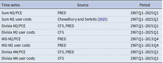
The quarterly data employed in this study span the period from 1967:Q1 to 2025:Q1 and are primarily obtained from two sources: the St. FRED databaseFootnote 5 and the CFS.Footnote 6 In addition, we use the dataset provided by Chowdhury and Serletis (Reference Chowdhury and Serletis2025) for the user costs associated with the simple-sum monetary aggregates. Data for MSI M2 and its user costs are obtained from FRED for the period 1967:Q1–2013:Q4. Table 1 summarizes the time series utilized in the empirical analysis and their respective data sources.
Time series definitions and sources

Table 1. Long description
A table with three columns and eight rows. The columns are labeled ‘Time series’, ‘Source’, and ‘Period’. The rows list different economic time series, their sources, and the periods for which the data is available. Row 1: Sum M2/PCE, FRED, 1967:Q1-2025:Q1. Row 2: Sum M2 user costs, Chowdhury and Serletis (2025), 1967:Q1-2025:Q1. Row 3: Divisia M2/PCE, CFS, FRED, 1967:Q1-2025:Q1. Row 4: Divisia M2 user costs, CFS, 1967:Q1-2025:Q1. Row 5: MSI M2/PCE, FRED, 1967:Q1-2013:Q4. Row 6: MSI M2 user costs, FRED, 1967:Q1-2013:Q4. Row 7: Divisia M4/PCE, CFS, FRED, 1967:Q1-2025:Q1. Row 8: Divisia M4 user costs, CFS, 1967:Q1-2025:Q1.
Note: This table presents the time series used in the empirical analysis. The quarterly time-series data cover the period from 1967:Q1 to 2025:Q1. CFS: Center for Financial Stability, FRED: Federal Reserve Economic Data, MSI: Monetary Services Index, PCE: Personal Consumption Expenditure.
4. The results
4.1. Calibrating copula
The conventional view holds that money demand is negatively correlated with user costs (Baumol, Reference Baumol1952; Tobin, Reference Tobin1956). Figure 1 displays a scatterplot of the simple-sum aggregate M2, scaled by PCE, against its user cost over the period 1967:Q1–2025:Q1. The fitted regression line indicates that, while the negative relationship holds on average, it appears to weaken in the region of low user costs, where the line does not fit money demand particularly well. This observation is consistent with recent empirical evidence suggesting that the relationship between money demand and user costs is not strictly negative (e.g., Benati et al., Reference Benati, Lucas, Nicolini and Weber2021; Gao et al., Reference Gao, Whited and Zhang2021; Movaghari and Sermpinis, Reference Movaghari and Sermpinis2025). Overall, these findings suggest that the empirical relationship between money demand and user costs is more complex than a purely linear specification would imply.Footnote 7 This complexity justifies the use of the copula function as a tool to model the overall dependence structure between the two variables. As highlighted by Hafner and Manner (Reference Hafner and Manner2012), ”A natural, and in fact the most general way to model nonlinear dependencies is to use copulas.”
This figure presents the scatterplot of simple-sum aggregate M2, scaled by PCE, against its user cost for the period 1967:Q1–2025:Q1. The blue line represent the fitted regression line with 95% confidence intervals.

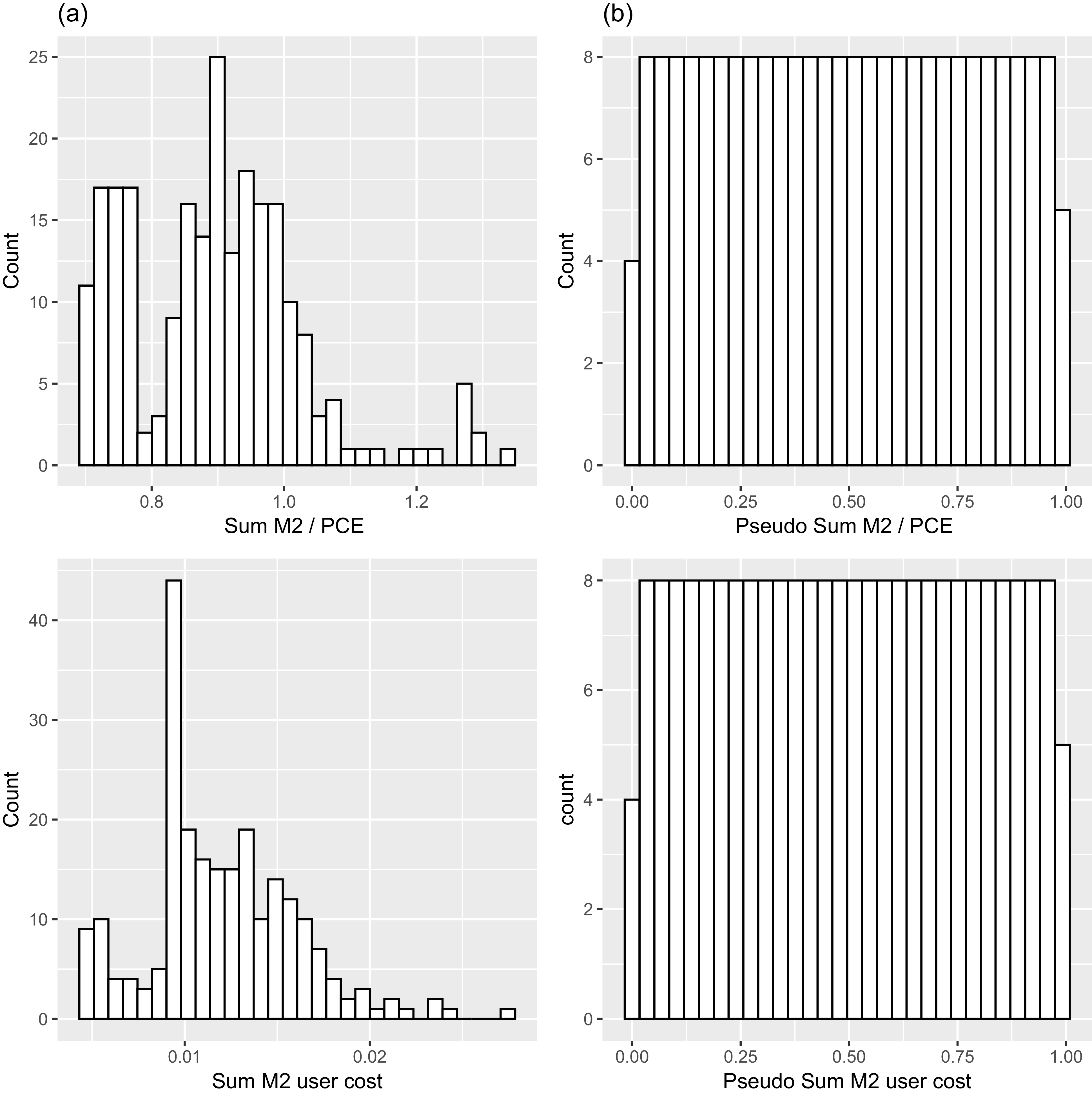
To prepare variables for copula modeling, the original data are transformed into a uniform distribution on the interval [0, 1] using the empirical distribution function (Breymann et al., Reference Breymann, Dias and Embrechts2003; Ruppert and Matteson, Reference Ruppert and Matteson2011). Figure 2 displays the distribution of the original data (Panel (a)) and the transformed pseudo-observations (Panel (b)). The first row presents the histogram of the Sum M2 time series, while the second row focuses on its user cost. The pseudo-observations are clearly uniformly distributed over the interval [0, 1]. Following this transformation, the copulas are fitted using a maximum pseudo-likelihood estimation method based on the resulting pseudo-observations (Breymann et al., Reference Breymann, Dias and Embrechts2003; Hofert et al., Reference Hofert, Kojadinovic, Maechler and Yan2024).
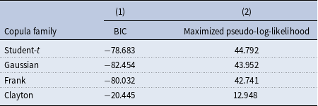
Next, we proceed to select the most suitable copula family. Following Ruppert and Matteson (Reference Ruppert and Matteson2011), we focus on two elliptical copulas, the Student-t and Gaussian copulas. The starting value for the copula parameter in the Gaussian family is taken to be the Kendall correlation coefficient. This non-parametric correlation is also used as the initial value for the Student-t copula parameter, along with 10 degrees of freedom. Furthermore, we consider two Archimedean copulas, namely the Clayton (Clayton, Reference Clayton1978) and Frank (Frank, Reference Frank1979) copulas. The main reason for examining these specific copulas is that certain copula families, such as Gumbel (Gumbel, Reference Gumbel1960) and Joe (Joe, Reference Joe1993), have limitations in modeling negatively dependent data (Ghosh et al., Reference Ghosh, Bhuyan and Finkelstein2022).Footnote 8 We follow Czado and Nagler (Reference Czado and Nagler2022) and identify the best copula family using Bayesian information criterion (BIC).
Copula family selection for the bivariate time series of simple-sum M2 and its user cost

Table 2. Long description
A table comparing copula families based on BIC and maximized pseudo-log-likelihood. The table has four rows and three columns. Column headers are Copula family, BIC, and Maximized pseudo-log-likelihood. Row labels are Student-t, Gaussian, Frank, and Clayton. Row 1: Student-t, -78.683, 44.792. Row 2: Gaussian, -82.454, 43.952. Row 3: Frank, -80.032, 42.741. Row 4: Clayton, -20.445, 12.948.
Note: This table presents the results of copula family selection for the bivariate time series of simple-sum aggregate M2 and its user cost for the period 1967:Q1–2025:Q1. The original data are transformed to uniformly distributed in [0, 1], then a maximum pseudo-likelihood estimation method based on these pseudo-observations is utilized to fitting copulas. Four common families are considered including Student-t, Gaussian, Frank, and Clayton. Bayesian information criterion (BIC) and the corresponding maximized pseudo-log-likelihood are reported in columns (1) and (2), respectively.
This figure illustrates the distribution of simple-sum aggregate M2 (upper panel), scaled by PCE, and its user cost (lower panel) for the period 1967:Q1–2025:Q1. Original and transformed pseudo-observations are depicted in panels (a) and (b), respectively.

Table 2 reports the BIC values for the four copula families under consideration. The results indicate that the Gaussian copula provides the best fit for the dependence structure between Sum M2 and its user cost, as it achieves the lowest BIC (–82.454). Although its maximized pseudo-log-likelihood is slightly lower than that of the Student-t copula (43.952 vs. 44.792), this contrast arises because the BIC criterion penalizes model complexity. The Student-t copula includes an additional parameter (degrees of freedom), which marginally improves fit but increases complexity. Once this penalty is taken into account, the Gaussian copula is preferred according to the BIC criterion. The superior performance of the Gaussian copula suggests that the dependence structure underlying M2 money demand can be adequately characterized by a conventional Gaussian-type dependence structure. This result indicates limited evidence of strong tail dependence or asymmetric dependence captured by alternative copula specifications. The selection of the Gaussian copula for the bivariate time series of Sum M2 and its user cost aligns with the results of Smith and Vahey (Reference Smith and Vahey2016). They demonstrate that Gaussian copula-based models are effective in capturing linear and nonlinear dependencies among U.S. macroeconomic variables.
4.2. Copula parameter estimation
As the second step, we summarize the dependence structure between money demand and its user cost into a univariate time series of copula parameters. For this purpose, we follow Movaghari et al. (Reference Movaghari, Serletis and Sermpinis2024) and estimate Gaussian copula parameters over 40-quarter rolling windows, corresponding to a decade-long time horizon. Table 3 presents the summary statistics of the estimated Gaussian copula parameters. The results show that the average correlation between Sum M2 and its user cost is strongly negative (–0.489), which is consistent with the prevailing view in the literature.
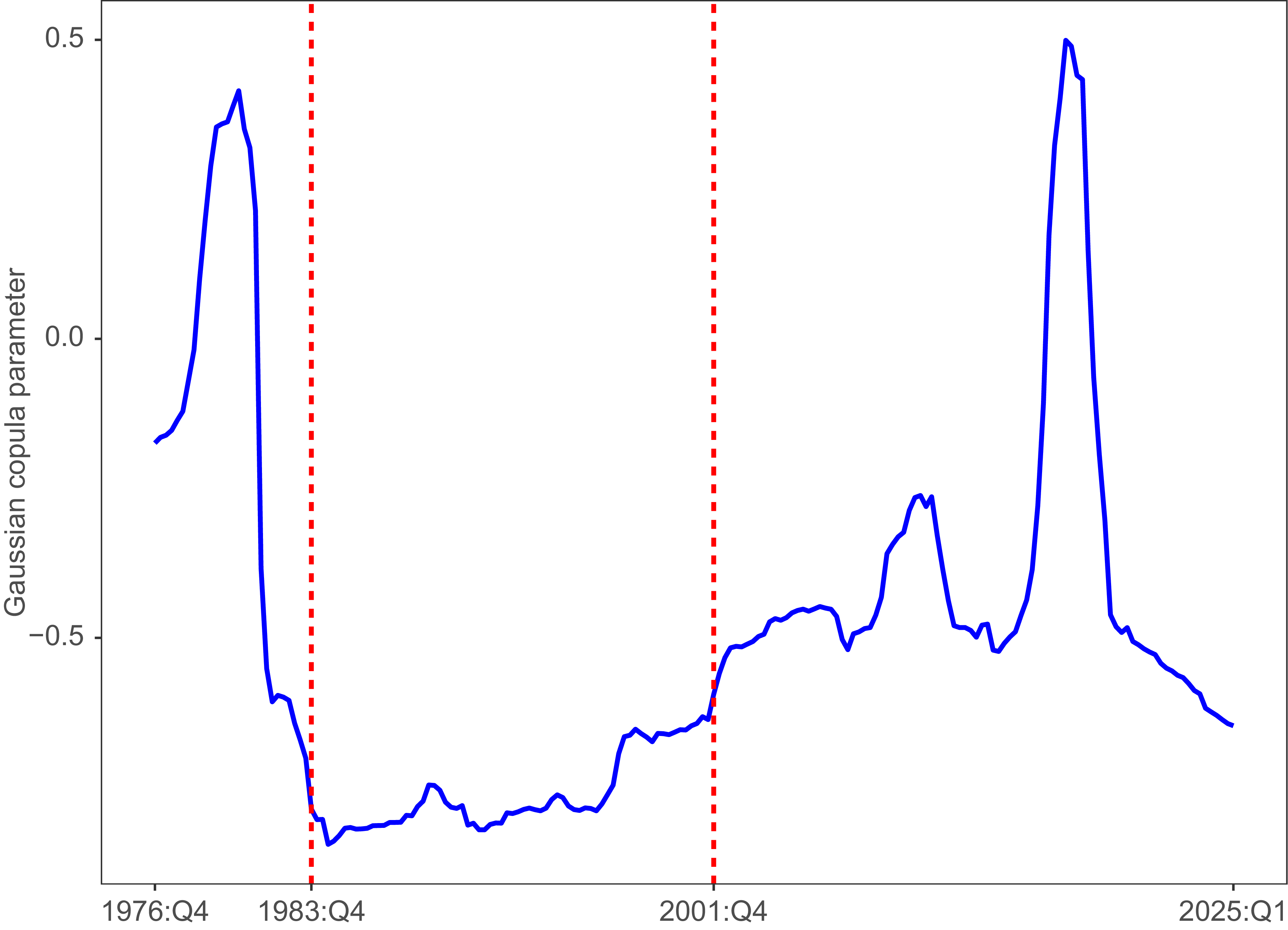
For a diagrammatical representation, we illustrate the time series plot of Gaussian copula parameters in Figure 3. As shown, the time series remains relatively stable between the mid-1980s and early 2000s. Outside this period, it fluctuates between positive and negative values.Footnote 9 The maximum copula parameter, 0.499, occurs in 2017:Q3, while the minimum copula parameter, −0.845, is observed in 1984:Q3. Broadly speaking, the time series plot of copula parameters suggest that the dependence structure of the money demand function evolves over time.
Summary statistics of Gaussian copula parameters for simple-sum measures

Table 3. Long description
A table summarizing statistics of Gaussian copula parameters over 40-quarter rolling windows. The table has one row and eight columns. The row label is 40-quarter rolling windows. The columns are No. of obs., Min, Q1, Median, Mean, Q3, Max, and SD. Row 1: No. of obs., 194; Min, -0.845; Q1, -0.766; Median, -0.530; Mean, -0.489; Q3, -0.448; Max, 0.499; SD, 0.329.
Note: This table presents the summary statistics of Gaussian copula parameters for the dependence structure between Sum M2 and its user cost. The copula parameters are estimated by the maximization of a pseudo-log-likelihood function over 40-quarter rolling windows.
4.3. Changepoints in the copula parameters
We have now reached the stage where potential changepoints in the dependence structure of the money demand function can be identified. We explore the structural break(s) in money demand function through the examination of the time series of copula parameter. We hypothesize that any break point(s) should be mirrored in the copula parameter.
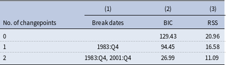
To achieve this, we employ the Bai and Perron (Reference Bai and Perron2003) structural break test to determine the timing of breaks in the time series of the Gaussian copula parameter. This methodology partitions the time series into distinct segments and evaluates whether significant changes occur in the underlying parameters across these segments. The optimal number of segments, and consequently the optimal number of changepoints, is determined by the minimum value of BIC (Zeileis et al., Reference Zeileis, Kleiber, Krämer and Hornik2003). Bai and Perron’s (Reference Bai and Perron2003) test is fundamentally a procedure that minimizes the residual sum of squares (RSS). To provide a clearer perspective on the performance of this analysis, we also report the RSS. Table 4 presents the results. According the minimum value of BIC, two changepoints are detected in the time series of Gaussian copula parameters at 1983:Q4 and 2001:Q4.
Changepoints in dependence structure between Sum M2 and its user cost

Table 4. Long description
A table with three columns and three rows. The columns are labeled as No. of changepoints, Break dates, BIC, and RSS. The rows present data for different numbers of changepoints: 0, 1, and 2. For 0 changepoints, BIC is 129.43 and RSS is 20.96. For 1 changepoint at 1983:Q4, BIC is 94.45 and RSS is 16.58. For 2 changepoints at 1983:Q4 and 2001:Q4, BIC is 26.99 and RSS is 11.09.
Note: This table reports the estimated break dates in the univariate time series of Gaussian copula parameters for the dependence structure between Sum M2 and its user cost. The Bai and Perron (Reference Bai and Perron2003) test is used to identify the number of breakpoints and their corresponding break dates. The parameters are estimated using 40-quarter rolling windows. The RSS and BIC are the residual sum of squares and Bayesian information criterion, respectively. The optimal number of changepoints is based on the minimum value of BIC.
This figure illustrates the time series plot of Gaussian copula parameters for the dependence structure between simple-sum aggregate M2 and its user cost. The parameters are estimated using 40-quarter rolling windows. Changepoints in the univariate time series of copula parameters are denoted by vertical dashed red lines at 1983:Q4 and 2001:Q4.

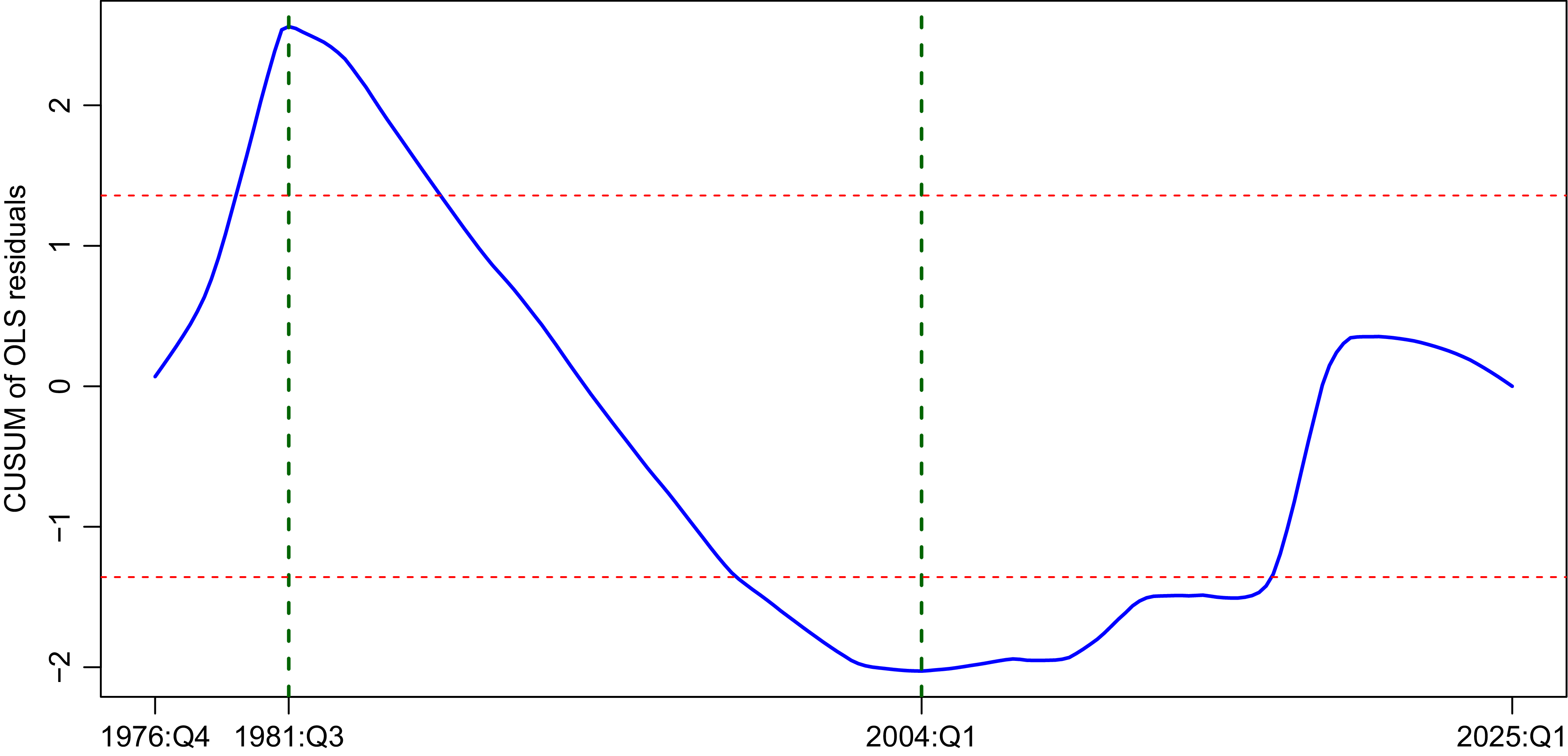
In a further analysis, and to ensure that the identified changepoints are not driven by the estimation approach, we re-estimate the copula parameters using rolling windows of length 35 and 45 and repeat the structural break tests. The results reported in Subsection 4.7 qualitatively support our main findings. To provide additional evidence, we apply the CUSUM procedure based on OLS residuals proposed by Ploberger and Krämer (Reference Ploberger and Krämer1992). Visual inspection of the CUSUM statistics can be informative for detecting structural breaks (Zakamulin and Hunnes, Reference Zakamulin and Hunnes2021). Figure 4 illustrates the CUSUM process for the Gaussian copula parameter of Sum M2. The horizontal red lines represent the asymptotic 5% critical boundaries derived from the Wiener process. The process exhibits two pronounced inflection points, marked by vertical green lines at 1981:Q3 and 2004:Q1. These turning points, with only minor discrepancies, closely align with the break dates identified using the Bai and Perron (Reference Bai and Perron2003) test. The fact that the process crosses the asymptotic 5% boundaries further underscores the statistical significance of these two breaks.
This figure illustrates the cumulative sum (CUSUM) process of the OLS residuals for the Gaussian copula parameter of Sum M2. The horizontal red lines represent the asymptotic 5% critical boundaries derived from the Wiener process. The vertical dashed lines indicate the maximum and minimum values of the CUSUM process.

Interestingly, the break dates in the copula parameters correspond to the beginning and end of the “Great Moderation,” a period from the mid-1980s to around 2000 characterized by unusually stable macroeconomic conditions (Belongia and Ireland, Reference Belongia and Ireland2016). It is plausible that these changes reflect shifts in Federal Reserve monetary policy during that time. Beginning in the mid-1980s, monetary policy placed increasing emphasis on controlling inflation, while around the early 2000s, the focus shifted back toward smoothing real economic fluctuations (Belongia and Ireland, Reference Belongia and Ireland2016; Clarida et al., Reference Clarida, Gali and Gertler2000; Lubik and Schorfheide, Reference Lubik and Schorfheide2004).
The two identified structural breaks are also important in other respects. First, the identified changepoint in the 1980s aligns with a significant transformation in the history of the U.S. banking system, specifically the phased repeal of Regulation Q between March 1980 and March 1986. Lucas and Nicolini (Reference Lucas and Nicolini2015) describe this period as a ”hectic period” characterized by substantial regulatory changes. Between 1933 and 1986, the Federal Reserve implemented Regulation Q, which imposed interest rate ceilings on time and savings deposits and prohibited interest on demand deposits (Koch, Reference Koch2015). This regulation was gradually phased out with the Deregulation Act of 1980, which began removing the interest rate ceilings. The process was completed by March 1986.
Second, compared to other decades, particularly the 1980s and 1990s, monetary policy in the 2000s has received relatively limited attention in the literature (e.g., Belongia and Ireland, Reference Belongia and Ireland2016; Clarida, Reference Clarida2012; Tchatoka et al., Reference Tchatoka, Groshenny, Haque and Weder2017). The detection of a changepoint in 2002 sheds new light on monetary policy during the 2000s, potentially offering insight into the question raised by Belongia and Ireland (Reference Belongia and Ireland2016), who stated, ”…raise the question of whether the United States, after an interlude spanning the mid-1980s through the 1990s, entered a period of renewed monetary instability after 2000.”
4.4. Evidence from Divisia measures
There has been strong debate regarding the suitability of traditional simple-sum monetary aggregates for examining money demand. For example, Schunk (Reference Schunk2001) states, “…the simple-sum aggregates have no meaning beyond simple accounting identities. In contrast, the Divisia monetary aggregates provide a theoretically valid measure of monetary services.” To address these concerns, Barnett (Reference Barnett1980) introduces the Divisia aggregation scheme as an alternative method for aggregating monetary assets.
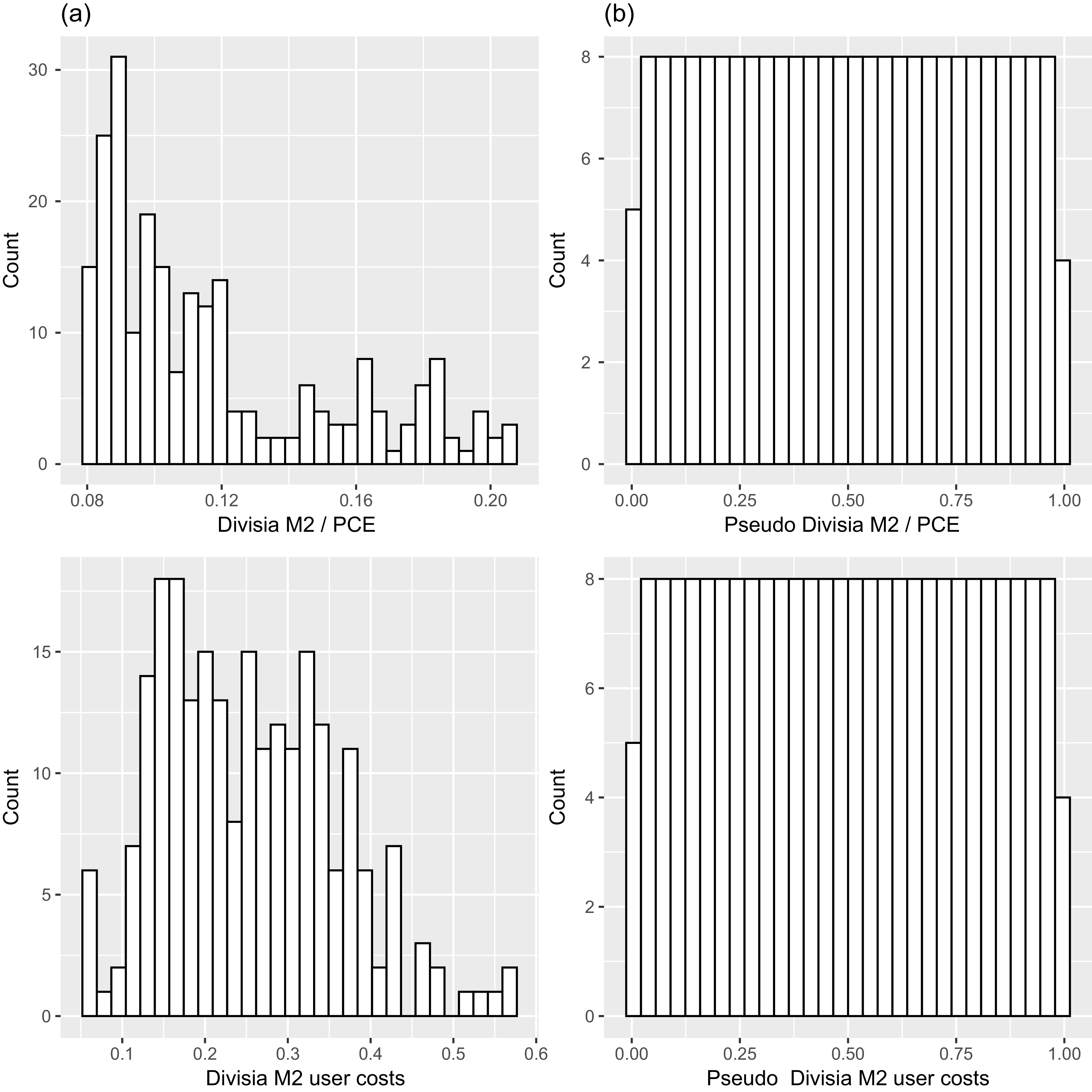
This figure illustrates the distribution of Divisia M2 (upper panel), scaled by PCE, and its user cost (lower panel) for the period 1967:Q1–2025:Q1. Original and transformed pseudo-observations are depicted in panels (a) and (b), respectively.

In this section, we replace the traditional simple-sum aggregate with its counterpart Divisia measure M2. This substitution serves two purposes. First, it enables us to test whether the identified changepoints remain consistent across different measures. Second, it allows us to examine the potential advantages of Divisia measures over traditional aggregates (e.g., Barnett et al., Reference Barnett, Offenbacher and Spindt1984; Bissoondeeal et al., Reference Bissoondeeal, Binner and Karoglou2023; Dery and Serletis, Reference Dery and Serletis2021; Jadidzadeh and Serletis, Reference Jadidzadeh and Serletis2019; Lucas, Reference Lucas2000). To provide additional evidence, we also examine the changepoint in the dependence structure of Divisia M4.
4.4.1. Copula family selection for Divisia measures
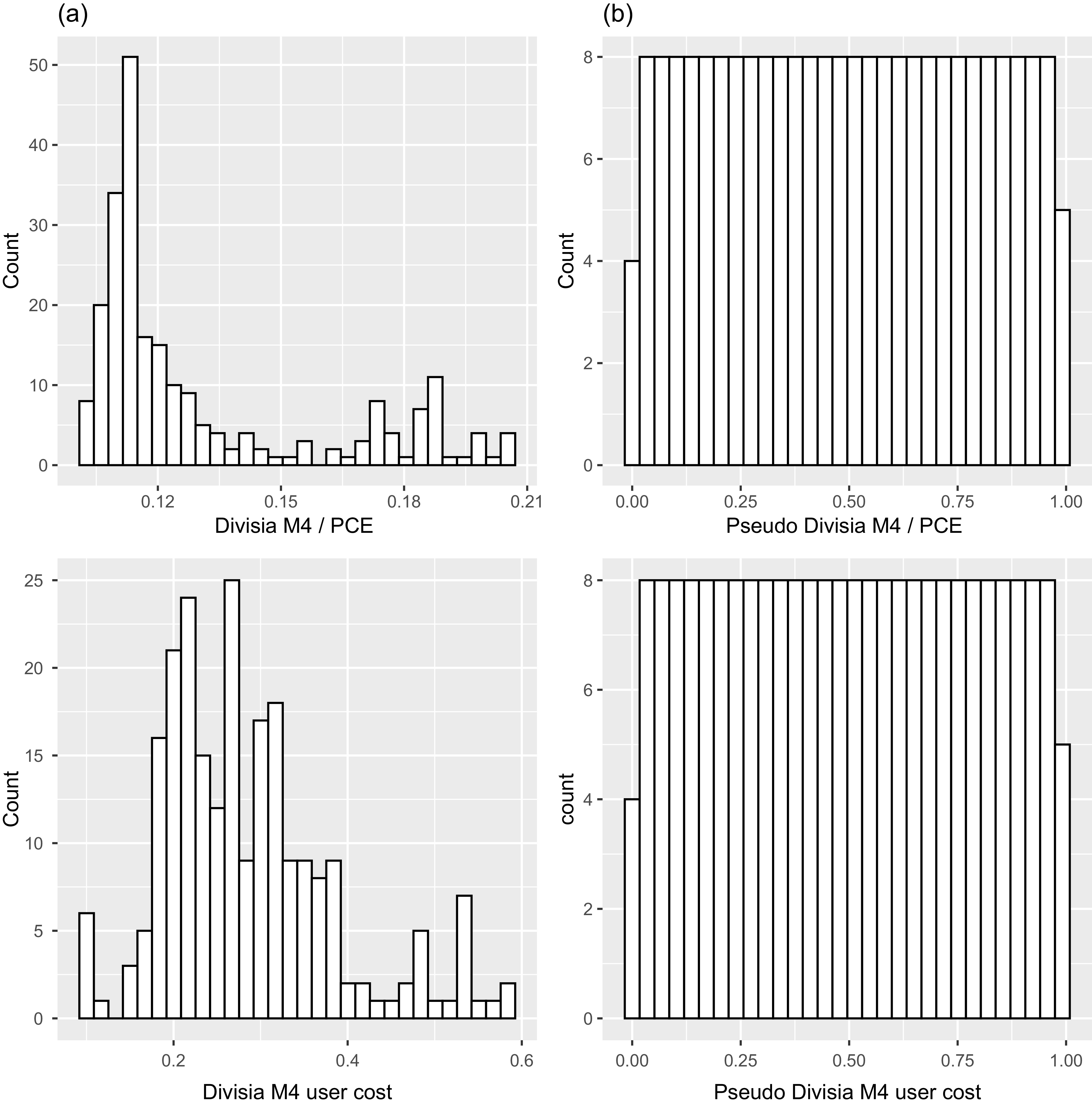
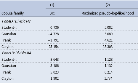
Following the procedure in the main analysis, we first transform the original data to a uniform distribution on the unit interval. Figures 5 and 6 illustrate the distributions of the original and transformed data for Divisia M2 and M4, respectively. We then select the copula family that best captures the dependence structure. Table 5 reports the BIC values and the corresponding maximized pseudo-log-likelihoods used to identify the most suitable copula family for capturing the dependence structure between Divisia ivisia M2 (Panel A) and Divisia M4 (Panel B) with their user costs. The results indicate that, unlike Sum M2, where elliptical copulas are best suited for modeling the dependence structure of the money demand function, Archimedean copulas perform better for Divisia monetary aggregates. In particular, the Clayton copula achieves the lowest BIC values of −25.154 and 1.902 in Panels A and B, respectively. It also exhibits the highest pseudo-log-likelihood among the copula families, with values of 15.303 and 1.774 in Panels A and B, respectively. Therefore, the Clayton copula is employed in the subsequent analysis to identify instabilities in the dependence structure of Divisia measures.
This figure illustrates the distribution of Divisia M4 (upper panel), scaled by PCE, and its user cost (lower panel) for the period 1967:Q1–2025:Q1. Original and transformed pseudo-observations are depicted in panels (a) and (b), respectively.

The preference for the Clayton copula in the Divisia aggregates specification suggests the presence of lower-tail dependence between money demand and user cost. Unlike the Gaussian copula, which assumes symmetric dependence and does not capture tail dependence, the Clayton copula allows the association between the variables to strengthen under extreme low-value conditions, taking into account the asymmetric dependence structure (e.g., Junker and May, Reference Junker and May2005; Yamaka et al., Reference Yamaka, Gupta, Thongkairat and Maneejuk2023). This finding implies that the Divisia-based money demand relationship may exhibit different dynamics during periods of unusually low user-cost conditions. Interestingly, Liu and Serletis (Reference Liu and Serletis2022) also find that credit card-augmented Divisia monetary aggregates exhibit lower-tail dependence between the demand for credit card transaction services and transaction balances.
4.4.2. Copula parameter estimation for Divisia measures
Table 6 presents the summary statistics of the estimated Clayton copula parameters. The obtained results indicate that both Divisia measures behave very similarly. On average, Divisia M2 and Divisia M4 exhibit moderate lower-tail dependence with their user costs. This implies that when user costs reach extremely low values, both Divisia M2 and M4 tend to decline as well. In terms of volatility, they also display similar magnitudes, with values of 0.733 and 1.209 for Divisia M2 and M4 copula parameters, respectively.
Copula family selection for the bivariate time series of Divisia measures and their user costs

Table 5. Long description
A table comparing copula families for Divisia measures and their user costs. The table has two panels, A and B, each with four rows and two columns. Panel A is for Divisia M2, and Panel B is for Divisia M4. The columns are labeled BIC and Maximized pseudo-log-likelihood. Panel A: Row 1: Student-t, 0.736, 5.082. Row 2: Gaussian, -4.728, 5.089. Row 3: Frank, -3.791, 4.621. Row 4: Clayton, -25.154, 15.303. Panel B: Row 1: Student-t, 8.643, 1.128. Row 2: Gaussian, 3.186, 1.132. Row 3: Frank, 5.023, 0.214. Row 4: Clayton, 1.902, 1.774.
Note: This table presents the results of copula family selection for the bivariate time series of Divisia M2 (Panel A) and Divisia M4 (Panel B) with their user costs for the period 1967:Q1–2025:Q1. The original data are transformed to uniformly distributed in [0, 1], then a maximum pseudo-likelihood estimation method based on these pseudo-observations is utilized to fitting copulas. Four common families are considered including Student-t, Gaussian, Frank, and Clayton. Bayesian information criterion (BIC) and the corresponding maximized pseudo-log-likelihood are reported in Columns (1) and (2), respectively.
Summary statistics of Clayton copula parameters for Divisia measures

Table 6. Long description
A table with two rows and nine columns comparing summary statistics of Clayton copula parameters for Divisia M2 and Divisia M4. The columns are labeled as No. of obs., Min, Q1, Median, Mean, Q3, Max, and SD. Row 1: Divisia M2, 194, -0.419, -0.269, -0.083, 0.274, 0.772, 2.539, 0.733. Row 2: Divisia M4, 194, -0.388, -0.226, 0.036, 0.697, 1.468, 4.130, 1.209.
Note: This table presents the summary statistics of Clayton copula parameters for the dependence structure between Divisia measures (M2 and M4) and their user costs. The copula parameters are estimated by the maximization of a pseudo-log-likelihood function over 40-quarter rolling windows.
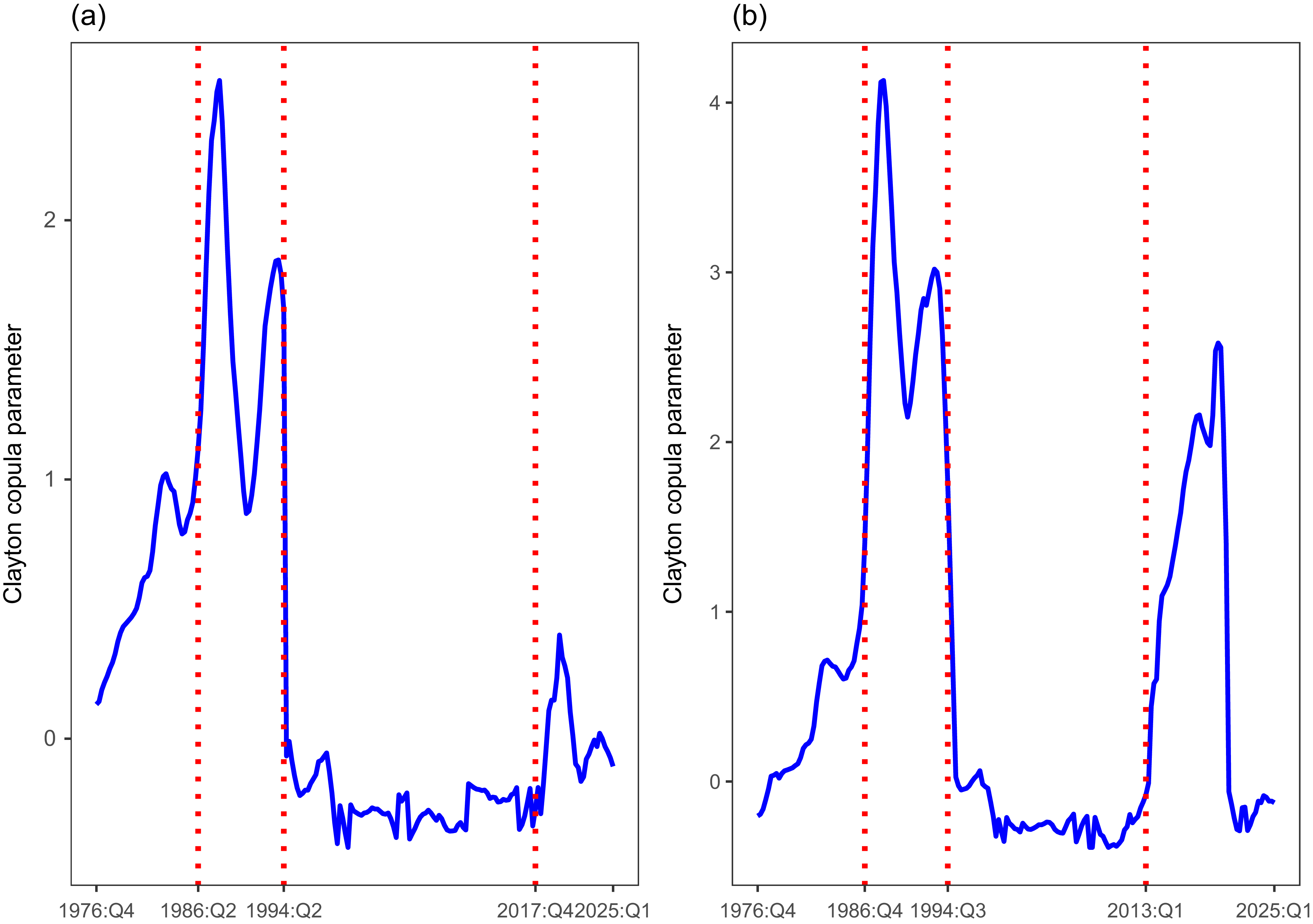
The similarity between the copula parameters of Divisia M2 and Divisia M4 is further highlighted by their time series plots. Figure 7 illustrates the time series of Clayton copula parameters for Divisia measures. Both time series illustrate a relatively dormant period in the Clayton parameter series. Specifically, between the mid-1990s and mid-2010s, the Clayton copula parameter remains stable around zero. In the following, we show that two structural changepoints occur at the beginning and end of this period.
Changepoints in dependence structure between Divisia measures and their user costs

Table 7. Long description
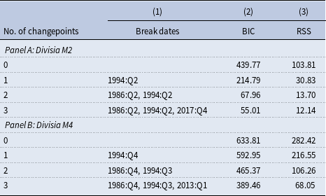
A table comparing changepoints in dependence structure between Divisia measures and their user costs. The table has three columns: No. of changepoints, Break dates, BIC, and RSS. It is divided into two panels: Panel A: Divisia M2 and Panel B: Divisia M4. Panel A: Divisia M2: Row 1: 0 changepoints, 439.77 BIC, 103.81 RSS. Row 2: 1 changepoint, 1994:Q2 break date, 214.79 BIC, 30.83 RSS. Row 3: 2 changepoints, 1986:Q2 and 1994:Q2 break dates, 67.96 BIC, 13.70 RSS. Row 4: 3 changepoints, 1986:Q2, 1994:Q2, and 2017:Q4 break dates, 55.01 BIC, 12.14 RSS. Panel B: Divisia M4: Row 1: 0 changepoints, 633.81 BIC, 282.42 RSS. Row 2: 1 changepoint, 1994:Q4 break date, 592.95 BIC, 216.55 RSS. Row 3: 2 changepoints, 1986:Q4 and 1994:Q3 break dates, 465.37 BIC, 106.26 RSS. Row 4: 3 changepoints, 1986:Q4, 1994:Q3, and 2013:Q1 break dates, 389.46 BIC, 68.05 RSS.
Note: This table reports the estimated break dates in the univariate time series of Clayton copula parameters for the dependence structure between Divisia M2 (Panel A) and Divisia M4 (Panel B) and their user cost. The Bai and Perron (Reference Bai and Perron2003) test is used to identify the number of breakpoints and their corresponding break dates. The parameters are estimated using 40-quarter rolling windows. The RSS and BIC are the residual sum of squares and Bayesian information criterion, respectively. The optimal number of changepoints is based on the minimum value of BIC.
This figure illustrates the time series plot of Clayton copula parameters for the dependence structure between Divisia M2 (Panel a) and Divisia M4 (Panel b) with their user costs. The parameters are estimated using 40-quarter rolling windows. Changepoints in the univariate time series of copula parameters are denoted by vertical dashed red lines.

4.4.3. Changepoints in copula parameters for Divisia measures
Table 7 presents the results of Bai and Perron’s (Reference Bai and Perron2003) test applied to the univariate time series of Clayton copula parameters of Divisia measures. Consistent with the main analysis, the copula parameters are estimated using 40-quarter rolling windows. Based on the minimum BIC values, three changepoints are identified in the dependence structure of both monetary aggregates. For Divisia M2, these occur at 1986:Q2, 1994:Q2, and 2017:Q4, while for Divisia M4, they are identified at 1986:Q4, 1994:Q3, and 2013:Q1. The first two changepoints are approximately identical, but the last one occurs in different years. Interestingly, the first changepoint in the mid-1980s (for both Divisia measures) coincides with the first changepoint identified for Sum M2.
Overall, there is a discrepancy in both the number and composition of the identified breakpoints between the simple-sum and Divisia monetary measures. This difference may reflect variations in both the set of monetary assets included in each aggregate and the method used to aggregate those assets. While simple-sum aggregates are constructed using straightforward accounting identities, Divisia measures are derived from the theoretical framework of index number theory (Schunk, Reference Schunk2001; Serletis, Reference Serletis1987).
The instabilities in the dependence structure of Divisia measures in the mid-1980s is consistent with prior evidence in the literature concerning the instability of Divisia measures following the banking deregulation of the 1980s (e.g., Bordo and Duca, Reference Bordo and Duca2025; Spencer, Reference Spencer1988). Another notable finding is the emergence of a changepoint in the mid-1990s, likely reflecting the influence of financial innovations of that decade. Ford et al. (Reference Ford, Peng and Mullineux1992) had already shown that Divisia monetary aggregates do not fully adjust for the effects of financial innovation. One such innovation was the introduction of sweep technology between January 1994 and April 1995 (Dutkowsky and Cynamon, Reference Dutkowsky and Cynamon2003). Under this system, commercial banks automatically shifted balances from checkable deposits into money market deposit accounts (MMDAs) at the close of business, transferring funds back when needed. These transfers were typically executed either at weekends or according to a pre-determined target balance (Teles and Zhou, Reference Teles and Zhou2005). Evidence from Berentsen et al. (Reference Berentsen, Huber and Marchesiani2015) indicates that the adoption of sweep technology substantially altered the money demand equilibrium. Similarly, Movaghari et al. (Reference Movaghari, Serletis and Sermpinis2024) attribute the changepoint they identify in the informational link between money demand and interest rates in the mid-1990s to the introduction of this technology.Footnote 10 Finally, we identify a changepoint in the relatively underexplored decade of the 2010s (2017:Q4 for Divisia M2 and 2013:Q1 for Divisia M4). The literature offers only limited analysis of monetary policy in this period (e.g., Wang, Reference Wang2024). This makes comparisons with prior studies difficult.
4.5. Which is more stable: simple-sum or Divisia aggregates?
At first glance, the higher number of breakpoints in the dependence structure between Divisia measures and their user costs, compared to the simple-sum measure (3 vs. 2), might suggest that simple-sum-based money demand is more stable than Divisia-based demand. But how strong is this stability? To address this question, we provide a graphical comparison between the three measures. Specifically, we examine the ACF of Gaussian and Clayton copula parameters for simple-sum M2 and Divisia measures, respectively. For a stationary time series, the ACF declines to zero relatively quickly, whereas for non-stationary data, it decays gradually (Hyndman and Athanasopoulos, Reference Hyndman and Athanasopoulos2018).
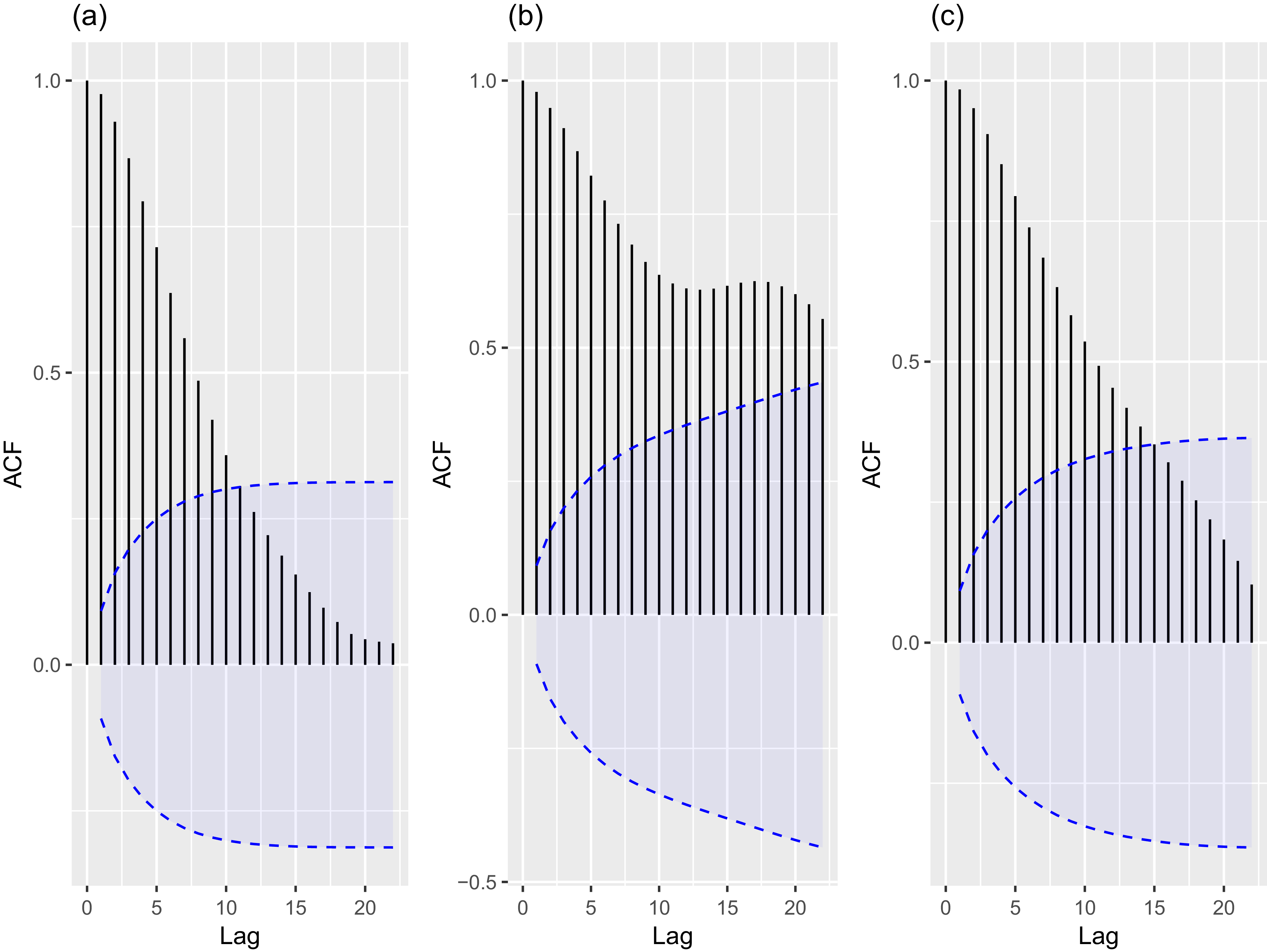
Figure 8 illustrates the ACF plots of the Gaussian and Clayton copula parameters. Panel (a) shows the ACF for the simple-sum-based copula parameters, while Panels (b) and (c) present the ACF for the Divisia-based parameters. The ACF plots suggest that Divisia M2 and Divisia M4 exhibit a slow decay in autocorrelation, whereas the autocorrelation function for Sum M2 declines more rapidly. In particular, the persistence is most pronounced for Divisia M2, which shows the slowest rate of decay among the series considered.
This figure presents the ACF plots of the copula parameters describing the dependence between monetary aggregates, Sum M2 (panel a), Divisia M2 (panel b), and Divisia M4 (panel c), and their user costs. The copula parameters for Sum M2 are estimated using a Gaussian copula, while Clayton copulas are employed for the Divisia measures. The 95% confidence intervals are shown as shaded blue bands.

The ACF-based comparison discussed above is purely visual. To provide more formal evidence on the relative stationarity of copula parameters for simple-sum and Divisia monetary aggregates, we conduct a series of numerical analyses.Footnote
11
First, to assess the persistence of dependence dynamics, we compute the half-life of shocks based on AR(1) representations of the copula parameters. The half-life of a shock is a simple transformation of AR(1) coefficient (
 $\rho$
) given by
 $\tau =\mathrm{log}(0.5) / \mathrm{log}(\rho )$
(Alvarez and Lippi, Reference Alvarez and Lippi2014). Then, we report unit root test statistics Augmented Dickey’Fuller (ADF; Dickey and Fuller, Reference Dickey and Fuller1979) and Kwiatkowski–Phillips–Schmidt–Shin (KPSS; Kwiatkowski et al., Reference Kwiatkowski, Phillips, Schmidt and Shin1992).
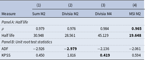
Table 8 presents the results. The estimated AR(1) coefficients are close to unity, implying relatively long half-lives. This finding suggests that adjustments in the dependence structure occur gradually and exhibit substantial persistence over time. Such persistence is not unexpected given the rolling-window estimation framework, which naturally smooths short-run fluctuations and generates overlapping estimates. The AR(1) coefficients for Divisia M2 and simple-sum M2 copula parameters are very close: 0.976 vs. 0.979. The implied half-lives vary from 28.6 quarters for Divisia M2 to 45.1 quarters for Divisia M4. These results suggest that shocks to the dependence structure in Divisia M2 dissipate more quickly than in other monetary aggregates, although the differences in persistence are modest. The unit root test statistics reported in Panel B provide contrasting evidence. The ADF test suggests that the dependence structure in Divisia M2 (with an ADF statistic of −2.979) is stationary relative to other measures. In contrast, the KPSS test indicates that the copula parameters of Divisia M4 (with a statistic of 0.419) are consistent with stationarity.
In the last column, we report results for MSI M2, a monetary aggregate adjusted to account for financial innovation in the mid-1990s. Our (unreported) results indicate that the Frank copula is the preferred specification according to the BIC criterion for capturing the dependence structure between MSI M2 and its user costs. The comparison of half-lives indicates that MSI M2 exhibits weaker persistence than Divisia M2 (19.648 versus 28.561), implying that shocks to MSI M2 fade out more rapidly, with their effects diminishing to half of the initial impact over a shorter period. These findings are consistent with the view that Anderson–Jones Divisia measures exhibit reduced persistence in response to shocks, including those potentially associated with institutional changes such as demand deposit sweep programs.
Stability measures in copula parameters

Table 8. Long description
The table presents stability measures in copula parameters for different monetary aggregates. It has four columns labeled Sum M2, Divisia M2, Divisia M4, and MSI M2, and two panels labeled Panel A: Half life and Panel B: Unit root test statistics. Panel A includes rows for ρ and Half life with corresponding values. Panel B includes rows for ADF and KPSS with corresponding values. The table compares the persistence and stationarity of the dependence structure in different monetary aggregates.
Note: This table reports stability measures for copula parameters describing the dependence structure between monetary aggregates and their user costs, including the AR(1) coefficient (
 $\rho$
) and half-life estimates (Panel A), as well as unit root test statistics (Panel B), namely the Augmented Dickey–Fuller (ADF) and Kwiatkowski–Phillips–Schmidt–Shin (KPSS) tests. Copula parameters for Sum M2 (Column (1)) are estimated using a Gaussian copula, while a Clayton copula is used for Divisia monetary aggregates (Column (2)-(3)). In Column (4), we present the results for the Monetary Services Index (MSI) M2 of Anderson and Jones (Reference Anderson and Jones2011), where the Frank copula is used to estimate the parameters. In each row, the monetary aggregate exhibiting more stationary behavior is shown in bold.
Overall, the findings suggest that no definitive conclusion can be drawn regarding the stability of the dependence structures between Sum M2 and Divisia measures. While some methods (e.g., the number of changepoints, ACF-based measures) indicate greater stability for simple-sum measures, others (e.g., half-life estimates) point to stronger stability in Divisia measures. These differences likely reflect the fact that the methods capture distinct aspects of dependence dynamics.
4.6. Copula parameters and macroeconomic regimes
The copula parameters used to identify instability in money demand are specified in an unconditional form. As a result, some of the structural breaks detected in the dependence measures may reflect changes in broader macroeconomic conditions rather than genuine instability in money demand itself.Footnote 12 To address this concern, we extend the analysis by investigating the determinants of the copula parameters within a time-series regression framework. Specifically, the estimated dependence measures are regressed on a set of macroeconomic regime indicators to assess whether changes in the dependence structure are systematically associated with shifts in the macroeconomic environment.
We consider three regime indicators: high inflation, recession periods, and the zero lower bound (ZLB) regime. Inflation is measured as the log change in the CPI obtained from the U.S. Bureau of Labor Statistics, and the high-inflation regime is defined based on the median inflation rate over the sample period. Recession periods are identified using the NBER business cycle dating chronology. Finally, the ZLB regime corresponds to the period during which the policy rate was constrained by the zero lower bound, particularly following December 2008 (e.g., Belongia and Ireland, Reference Belongia and Ireland2018; Jadidzadeh and Serletis, Reference Jadidzadeh and Serletis2019).
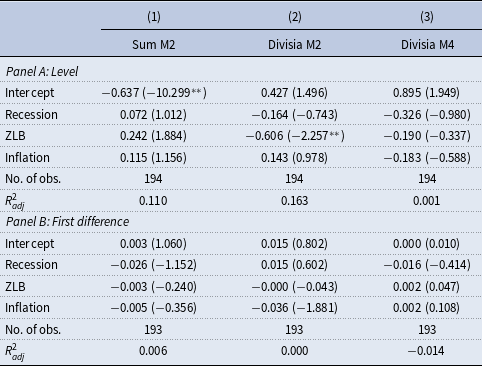
Table 9 reports the estimation results. To account for potential heteroskedasticity and serial correlation in the residuals of the time-series regressions, we employ Newey–West heteroskedasticity and autocorrelation consistent (HAC) standard errors to ensure valid statistical inference (Newey and West, Reference Newey and West1987). Since the estimated copula parameters exhibit a high degree of persistence, with significant autocorrelation extending beyond 10 lags, we adopt a relatively large HAC bandwidth of 15. The lag length is kept constant across all monetary aggregates for comparability. To further address potential inference issues arising from persistence, we also estimate the regressions in both levels (Panel A) and first differences (Panel B), following Graham and Leary (Reference Graham and Leary2018). For the first-difference specification, the HAC bandwidth is reduced to 5.
Macroeconomic regime effects on estimated copula parameters

Table 9. Long description
A table with two panels (A and B) showing regression results for macroeconomic regime effects on estimated copula parameters. Panel A presents results in levels, while Panel B presents results in first differences. Each panel has three columns representing different monetary aggregates: Sum M2, Divisia M2, and Divisia M4. The table includes rows for Intercept, Recession, ZLB, Inflation, Number of observations, and R-squared values. Each cell contains regression coefficients with t-statistics in parentheses. Notable trends include significant coefficients for Intercept in Panel A and varying effects of Recession, ZLB, and Inflation across different monetary aggregates.
Note: This table reports second-stage regression results examining the relationship between estimated copula parameters and macroeconomic conditions. The dependent variable is the 40-quarter rolling-windows copula dependence parameter. Copula parameters for Sum M2 (Column (1)) are estimated using a Gaussian copula, while a Clayton copula is used for Divisia monetary aggregates (Column (2)–(3)). The regressions are estimated in levels (Panel A) and first differences (Panel B). Explanatory variables include a recession dummy based on the NBER business cycle dating, high inflation rate regime, and a zero lower bound (ZLB) indicator. The regressions are estimated separately for three monetary aggregates: Sum M2, Divisia M2, and Divisia M4. Standard errors are computed using the heteroskedasticity and autocorrelation consistent (HAC) estimator of Newey and West (Reference Newey and West1987) to account for serial correlation induced by rolling-window estimates. t-statistics are reported in parentheses. **denotes significance at the 5% level.
Examining the estimation results in levels (Panel A) reveals that neither the recession dummy nor the high-inflation dummy has a statistically significant effect on any of the monetary aggregates. The only exception is the ZLB dummy, which exhibits a statistically significant effect at the 5% level on the Clayton copula parameter for Divisia M2. However, this result should be interpreted with caution, as the bandwidth of fifteen lags employed for the HAC estimator may still be insufficient for Divisia M2, whose autocorrelation function remains highly persistent even after 20 lags (see Figure 8). The estimation results using first differences, reported in Panel B, further confirm that none of the macroeconomic indicators exerts a statistically significant effect on the copula parameters. The general conclusion drawn from the analysis in this section is that macroeconomic regime variables are generally insignificant, suggesting that the detected shifts in dependence are unlikely to be solely driven by broader macroeconomic conditions.
4.7. Alternative window lengths
There is a concern that the main results may be biased due to the subjective determination of the window length (40 quarters) in the rolling procedure for copula parameter estimation. To evaluate the sensitivity of the identified changepoints to the window length, we analyze results using shorter (35 quarters) and longer (45 quarters) window lengths.
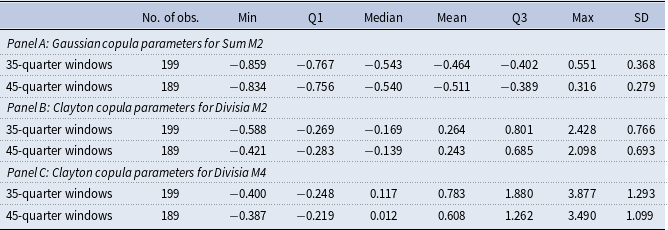
Table 10 reports the summary statistics for the Gaussian and Clayton copula parameters, estimated over 35- and 45-quarter rolling windows as alternative lengths in the time-varying copula framework. Panel (A) characterizes the dependence structure between Sum M2 and its user cost, while Panel (B) presents the results for Divisia measures. On average, the estimated copula parameters for the simple-sum monetary aggregate are −0.464 and −0.511 for the 35- and 45-quarter rolling windows, respectively. These values are very close to the average of −0.489 obtained using the 40-quarter window in the main analysis. A similar pattern is observed for Divisia measures in Panel (B). These results indicate that our main findings are robust to the choice of rolling window length in the copula parameter estimation.
Summary statistics of copula parameters: Alternative window lengths

Table 10. Long description
The table presents summary statistics for copula parameters for the dependence structure between Sum M2, Divisia M2, and Divisia M4 with their respective user costs. It includes data for 35-quarter and 45-quarter rolling windows. Panel A shows Gaussian copula parameters for Sum M2, Panel B shows Clayton copula parameters for Divisia M2, and Panel C shows Clayton copula parameters for Divisia M4. Each panel includes columns for the number of observations, minimum, first quartile (Q1), median, mean, third quartile (Q3), maximum, and standard deviation (SD). Panel A: Gaussian copula parameters for Sum M2. 35-quarter windows: 199 observations, minimum -0.859, Q1 -0.767, median -0.543, mean -0.464, Q3 -0.402, maximum 0.551, SD 0.368. 45-quarter windows: 189 observations, minimum -0.834, Q1 -0.756, median -0.540, mean -0.511, Q3 -0.389, maximum 0.316, SD 0.279. Panel B: Clayton copula parameters for Divisia M2. 35-quarter windows: 199 observations, minimum -0.588, Q1 -0.269, median -0.169, mean 0.264, Q3 0.801, maximum 2.428, SD 0.766. 45-quarter windows: 189 observations, minimum -0.421, Q1 -0.283, median -0.139, mean 0.243, Q3 0.685, maximum 2.098, SD 0.693. Panel C: Clayton copula parameters for Divisia M4. 35-quarter windows: 199 observations, minimum -0.400, Q1 -0.248, median 0.117, mean 0.783, Q3 1.880, maximum 3.877, SD 1.293. 45-quarter windows: 189 observations, minimum -0.387, Q1 -0.219, median 0.012, mean 0.608, Q3 1.262, maximum 3.490, SD 1.099.
Note: This table presents summary statistics for copula parameters for the dependence structure between Sum M2 (Panel A), Divisia M2 (Panel B) and Divisia M4 (Panel C) with their respective user costs. In each panel, the copula parameters are re-estimated using 35- and 45-quarter rolling windows, serving as alternative lengths in the rolling time-varying copula framework. The parameter estimates are obtained through the maximization of a pseudo-log-likelihood function.
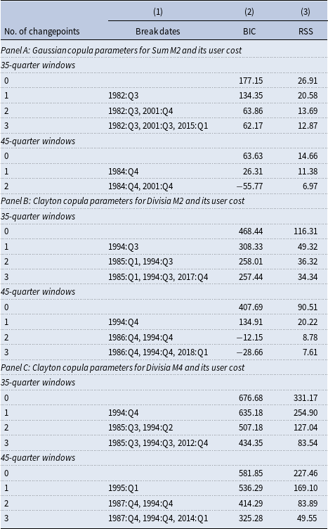
To further examine the robustness of our results, we investigate the impact of rolling window length on the estimated break dates in the univariate time series of copula parameters. Table 11 reports the results of Bai and Perron’s (2003) tests for identifying break dates based on alternative window lengths, namely 35- and 45-quarter rolling windows. Panel (A) presents the results for the Gaussian copula parameters, which characterize the dependence structure between Sum M2 and its user cost, while Panel (B) focuses on Divisia measures. The analysis using 45-quarter rolling windows confirms the changepoints identified in the 40-quarter-based analysis. Specifically, two changepoints are detected in the dependence structure between Sum M2 and its user cost, occurring in the mid-1980s and early 2000s. In addition, the 35-quarter-based results largely support our main findings, revealing the same two changepoints in the 1980s and 2000s, along with an additional breakpoint in the mid-2010s. The results reported in Panel (B) similarly confirm our findings regarding the number and timing of breakpoints in the dependence structure between Divisia M4 and its user cost. These results indicate that the timing of instabilities in the dependence structure of the money demand function is robust to variations in the window length used for estimating the copula parameters.
Changepoints in dependence structure between broad aggregates and their user costs: Alternative window lengths

Table 11. Long description
A table with three panels (A, B, and C) comparing changepoints in dependence structure between broad aggregates and their user costs using 35- and 45-quarter windows. Panel A: Gaussian copula parameters for Sum M2 and its user cost. Panel B: Clayton copula parameters for Divisia M2 and its user cost. Panel C: Clayton copula parameters for Divisia M4 and its user cost. Each panel lists the number of changepoints, break dates, BIC, and RSS values. Panel A shows results for 35- and 45-quarter windows with varying numbers of changepoints and corresponding break dates. Panel B and Panel C follow a similar structure, presenting results for Divisia M2 and Divisia M4 respectively. The table aims to examine the robustness of the results by investigating the impact of rolling window length on the estimated break dates in the univariate time series of copula parameters.
Note: This table reports the estimated break dates in the univariate time series of copula parameters, obtained using alternative window lengths of 35 and 45 quarters. The Gaussian copula is employed to model the dependence between Sum M2 and its user cost in Panel A, while the Clayton copula is used for Divisia M2 and Divisia M4 in Panels B and C, respectively. In each panel, we re-run the Bai and Perron’s (2003) test for 35- and 45-quarter rolling windows. The RSS and BIC are the residual sum of squares and Bayesian information criterion, respectively. The optimal number of changepoints is based on the minimum value of BIC.
4.8. Does functional form matter?
In examining money demand function stability, three classic specifications are proposed in the literature, including log–log (Meltzer, Reference Meltzer1963), the semi-log (Cagan, Reference Cagan1954), and the Selden-Latané (Selden, Reference Selden1956; Latané, Reference Latané1960) specifications.Footnote 13 In the log–log specification, both money balances and their corresponding user costs are log-transformed in the money demand function. In contrast, the semi-log specification applies the logarithmic transformation only to money balances, leaving the user cost in its original (non-log) form. In the Selden–Latané specification, the velocity of the monetary aggregate (the inverse of the appropriately scaled monetary aggregate) is linked to the raw user cost (see, Belongia and Ireland, Reference Belongia and Ireland2019, for example).
In this section, we assume that the data-generating process (DGP) underlying the components of the money demand function conforms to classical specifications. This naturally raises the question of whether our copula-based results are sensitive to this assumption. To address this, we draw on the invariance property of copulas under strictly monotonic transformations (e.g., Nelsen, Reference Nelsen2006). This property implies that transforming one or both time series in a bivariate system using a strictly monotonic function does not alter the underlying dependence structure captured by the copula. Therefore, applying transformations such as logarithms (in log–log or semi-log specifications) or inversion (as in the Selden–Latané specification) does not affect the dependence structure and thus does not change the results derived from the raw components of the money demand function.
5. Conclusion
Studies examining the stability of the money demand function are typically based on regression models, where linearity is considered one of the fundamental assumptions. In this study, we examine the stability of the money demand function with a holistic approach, utilizing the capabilities of copula methods. Specifically, we employ the copula technique to explore potential breakpoints in the overall dependence structure between monetary aggregates and their user costs, rather than focusing solely on linear dependencies.
Our findings suggest that when modeling the dependence structure of the money demand function, elliptical copulas are more appropriate for traditional simple-sum monetary aggregates, while Archimedean copulas provide a better fit for Divisia-based measures. By conducting changepoint analysis on the copula parameter time series, we identify two changepoints in the dependence structure of Sum M2, compared to three changepoints for Divisia measures. Both measures exhibit a changepoint in the 1980s, coinciding with a period of significant regulatory changes. In more recent decades, the simple-sum measure shows a changepoint in the early 2000s, whereas the Divisia measure exhibits one in the early 2010s. Additionally, the Divisia measure presents a changepoint in the mid-1990s, potentially reflecting the impact of financial innovations during that decade.
One notable implication of our findings is that the copula-based evidence does not support the claimed superiority of Divisia measures over simple-sum measures, as suggested in the literature. In fact, even Sum M2 appears to exhibit somewhat more stability than Divisia M4. An examination of the ACF of the copula parameters reveals that the stability of the money demand dependence structure is broadly similar for both measures at least across the initial lags.
The unexpectedly weak performance of the Divisia measures in terms of the stability of the correlation structure raises the question of whether incorporating deferred-payment transaction services provided by credit cards could improve the stability of the Divisia correlation structure. In a recent study, Chowdhury and Serletis (Reference Chowdhury and Serletis2025) show that the original Divisia aggregates are not stable based on the Pesaran et al. (Reference Pesaran, Shin and Smith2001) bounds testing procedure. However, when they focus on the post-2006 period, during which credit-augmented Divisia monetary aggregates are available, they find that money demand is stable with both the original and the credit-augmented Divisia aggregates. As a potential avenue for future research, we therefore suggest applying copula techniques to the dependence structure of credit-augmented Divisia monetary aggregates to evaluate whether money demand dependence performs better under this specification.
Acknowledgements
Special thanks are due to Fredj Jawadi (the special issue editor), and William A. Barnett (the editor), and two anonymous reviewers for highly constructive comments and suggestions that have helped to significantly improve the quality of the paper. We also gratefully acknowledge helpful comments from the audiences at the 10th Annual Conference of the Society for Economic Measurement (SEM), Athens University of Economics and Business.
Appendix A. R code










 Open access

