














1. Introduction
Despite being the first type of exoplanet to be discovered around a main-sequence star (Mayor & Queloz Reference Mayor and Queloz1995), hot giant planets (M
 $_{p}$
 $\gtrsim$
0.3
 $M_{J}$
,
 $P \lt 10$
days) continue to challenge our understanding of planet formation and evolution. Although it is widely accepted that orbital migration is necessary to move these planets from their formation locations beyond the snowline to their current close-in orbits, the exact mechanisms are still contested (Dawson & Johnson Reference Dawson and Johnson2018). The two predominant theories are high-eccentricity migration (HEM) and disk-driven migration. In the first scenario, planets are perturbed to an eccentric orbit by the gravitational influence of an outer body (such as another planet or a stellar companion, known as Kozai–Lidov oscillations), secular interactions or planet-planet scattering (e.g. Naoz Reference Naoz2016; Adams & Laughlin Reference Adams and Laughlin2006; Ford & Rasio Reference Ford and Rasio2008). Tidal interactions with the host star during close approaches at periastron then circularise and shrink the orbit. Whilst the majority of hot giants are observed to have circular orbits, a non-negligible fraction remain eccentric (i.e. are in the midst of this process) with a distribution consistent with HEM (e.g. Bonomo et al. Reference Bonomo2017). For instance, many systems hosting hot Jupiters (HJs) have also been found to contain outer gas giant companions, with their HJs possessing higher average eccentricities than those in single planet systems (Knutson et al. Reference Knutson2014; Bryan et al. Reference Bryan2016). Furthermore, the shape of the upper boundary of the sub-Jovian desert (a dearth of giants in a region of the close-in planet parameter space) also lends support to the HEM theory (see Owen & Lai Reference Owen and Lai2018).
The second scenario of disk-driven migration results from the exchange of angular momentum and energy between an embedded planet and protoplanetary disk (Goldreich & Tremaine Reference Goldreich and Tremaine1980). Depending upon the presence of gaps in the disk, along with the viscosity and scale height, this mechanism can result in the rapid inward (or outward) migration of a planet (see Baruteau et al. Reference Baruteau, Beuther, Klessen, Dullemond and Henning2014). Disk-driven migration may be more relevant to circularised and mildly eccentric warm Jupiters (WJs,
 $10 \lt P \lt 200$
days), as it is not fully consistent with the mass and eccentricity distributions of HJs observed (Petrovich & Tremaine Reference Petrovich and Tremaine2016). However, the existence of multi-planet systems with close companions to HJs indicates that this process must occur in some cases, as a highly dynamical pathway such as HEM would disrupt the architecture of these systems (e.g. Becker et al. Reference Becker, Vanderburg, Adams, Rappaport and Schwengeler2015; Huang et al. Reference Huang2020b). It may be that both migration mechanisms are required (with differing probabilities) to reproduce the trends observed in the short-period giant population (Dawson & Johnson Reference Dawson and Johnson2018).
Since the launch of the Transiting Exoplanet Survey Satellite (TESS, Ricker et al. Reference Ricker2015) in 2018, hundreds of new close-in giant planet candidates have been announced around the Solar neighbourhood (
 $d \lt 1$
kpc). With an increasing number of well-characterised giants with accurate host star parameters, we can now assess the influence of host stars on the evolution of this class of planets. Of particular interest are systems with young to intermediate age stars (
 $T \lt 1$
Gyr) and post-main sequence stars, as these populations were sparsely studied in the era of the Kepler mission (Borucki et al. Reference Borucki2010) and are vital for understanding the radius inflation of HJs and other close-in giants (e.g. Weiss et al. Reference Weiss2013; Sarkis et al. Reference Sarkis, Mordasini, Henning, Marleau and Mollière2021). Comparisons between the occurrence rates of giant planets around different stellar populations (such as low-mass, thin/thick disk, halo and those in stellar clusters) may also expose the circumstances of their formation and evolution in greater detail (e.g. Newton et al. Reference Newton2019; Kanodia et al. Reference Kanodia2024). Furthermore, the James Webb Space Telescope (JWST, Gardner et al. Reference Gardner2006) and the upcoming Ariel mission (Tinetti et al. Reference Tinetti, MacEwen, Fazio, Lystrup, Batalha, Siegler and Tong2016) will allow us to probe the atmospheric compositions of a large sample of giant planets through transmission spectroscopy. Certain chemical signatures, such as the C/O ratio (a tracer of birth location), may remain from formation and allow us to discriminate between possible origin scenarios (see Mordasini et al. Reference Mordasini, van Boekel, Mollière, Henning and Benneke2016; Wang et al. Reference Wang, Changeat, Tinetti, Turrini and Wright2023). Hence, it remains vital to perform follow-up on giant planet candidates from TESS in order to validate and characterise interesting targets for these missions.
The ‘TASmanian Search for Inclined Exoplanets’ (TASSIE) program aims to study transiting (i.e. inclined) planets in the sub-Jovian desert alerted by the TESS mission, along with other hot giants in the southern sky (for further details, see Plunkett et al. Reference Plunkett2025). In this work, we present three new giant planet candidates alerted by TESS and investigated with the Harlingten 50 cm telescope at University of Tasmania Greenhill Observatory (UTGO). The paper is organised as follows. In Section 2, we detail the observations of these system including ground-based follow-up photometry from UTGO, reconnaissance spectroscopy, high angular resolution speckle imaging and high-precision RV measurements. In Section 3, we derive the stellar characteristics from spectroscopic analysis and spectral energy distribution fitting. We then move on to planet validation in Section 4 using archival imaging, astrometry and statistical testing with TRICERATOPS (Giacalone et al. Reference Giacalone2021). We then perform joint modelling of the light curves and RVs with Juliet (Espinoza et al. Reference Espinoza, Kossakowski and Brahm2019). In Section 5, we discuss the three systems in the context of the short-period planet population and suggest future observations. Finally, we present our conclusions in Section 6.
2. Observations
As part of the TASSIE program, these targets were selected for follow-up from the TESS Object of Interest (TOI) sample following the criteria outlined in Plunkett et al. (Reference Plunkett2025). We now detail the observations collected for each system.
2.1. Photometry
We obtained the TESS data, including the Target Pixel Files (TPFs), Full Frame Images (FFIs) and light curves from the Mikulski Archive for Space Telescopes (MAST). For two of the targets, we found that the light curves for some sectors were unavailable (or were from inconsistent pipelines) when searching through the Lightkurve package (Lightkurve Collaboration et al. Reference Collaboration2018). To ensure that the light curve analysis and derived transit depths were unbiased by these differing extractions, we decided to create our own light curves for two of the targets from their FFIs using the TESS-GAIA Light Curve (TGLC) package (Han & Brandt Reference Han and Brandt2023). This package utilises Gaia DR3 (Gaia Collaboration et al. 2023) photometry and astrometry to forward model the FFIs, building a per-image effective point spread function (ePSF). This has been shown to produce better photometric precision and more accurate de-blending, especially for faint targets.
We performed ground-based follow-up observations primarily with the Harlingten 50 cm (H50) telescope at the University of Tasmania Greenhill Observatory (UTGO). This was done to confirm the source of the transit, rule out false positives (such as eclipsing binaries and stellar activity) and refine the orbital ephemerides. The H50 is equipped with an Apogee ALTA U42 CCD camera, with a pixel scale of 0.8 arcsec pix
 $^{-1}$
and a 27.2
 $^{\prime}$
 $\times$
27.2
 $^{\prime}$
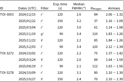
field-of-view. Data were reduced and differential photometry was extracted by a custom pipeline utilising the Prose package (Garcia et al. Reference Garcia2022). The logs of the H50 observations are shown in Table 1, with logs for the additional ground-based photometry in the Appendix (Table A1). We now describe the observations for each target in greater detail.
Observation logs for TASSIE II TOIs using the H50 telescope.

Table 1. Long description
The table presents observation logs for TASSIE II TOIs using the H50 telescope. It has six columns: ID, Dates (UTC), Filter, Exp. time (s), Median FWHM (arcsec), N images, and Airmass. The table includes data for three TOIs: TOI-3053, TOI-3272, and TOI-3278. Each row lists the observation details for a specific date and filter. For TOI-3053, observations are listed for six different dates with varying filters (r, g, V, i), exposure times, median FWHM, number of images, and airmass values. TOI-3272 has observations for three dates with filters r, V, and i. TOI-3278 has observations for two dates with filters r and V.
2.1.1. TIC 269859655 – TOI-3053
TIC 269859655 is a
 $V \approx 13.2$
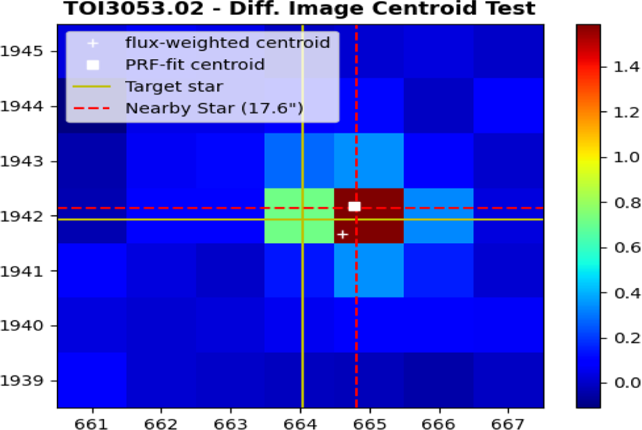
mag star in the constellation of Carina. It was observed by TESS in Sectors 9, 10, 11, 36, 37, 38, 64 and 90 at cadences ranging from 1 800 s down to 200 s. Raw photometric data were processed by the TESS Quick Look Pipeline (QLP, Huang et al. Reference Huang2020a), which performs difference imaging photometry, preliminary de-trending of instrumental effects and flux de-blending. TOI-3053 was originally flagged as a community TOI in Olmschenk et al. (Reference Olmschenk2021) and then recovered by the TESS Faint Star Search (Kunimoto et al. Reference Kunimoto2022), with a candidate signal found at a period of 2.991 days and a large depth of 17.1 parts per thousand (ppt). We validate this signal with our own Box Least Squares (BLS, Kovács et al. Reference Kovács, Zucker and Mazeh2002) search, but also found an additional candidate signal at
 $\approx$
0.416 days with a depth of
 $\approx$
2 ppt. However, after performing a difference image centroid test,Footnote
a
we determined the signal was offset from the target star by roughly 17
 $^{\prime\prime}$
(as shown in Figure A1). This likely indicates that this short-period signal is a blended eclipsing binary that is aligned to this target.
We observed one nearly complete transit of TOI-3053.01 on 2024/12/15 with exposures of 120 s in the SDSS
 $r^{\prime}$
filter. Imaging was disrupted by a potential time critical transient, but this alert was soon retracted and observations recommenced. The conditions were clear with moderate winds at 13 km h
 $^{-1}$
. We observed TOI-3053.01 again on 2025/11/19, 2025/11/22 and 2025/12/03 with the SDSS
 $g^{\prime}$
, Bessell V and SDSS
 $i^{\prime}$
filters, respectively, to check the transit depth was achromatic (discussed further in Section 4.1.3). Further information on each session is shown in Table 1. To confirm that the 0.416 day signal was a false positive, we also observed during the potential eclipse times on 2025/02/22 (assuming the full period) and 2025/03/04 (assuming half the period). We found a deep 20 ppt dip on a close F-dwarf in the first epoch, consistent with a de-blended depth estimate from the TESS light curves and Gaia DR3 fluxes. We therefore rule this out as a signal and treat this as a single candidate system.
Two additional light curves were obtained for TOI-3053, as part of the TESS Follow-up Observing Program Sub Group 1Footnote
b
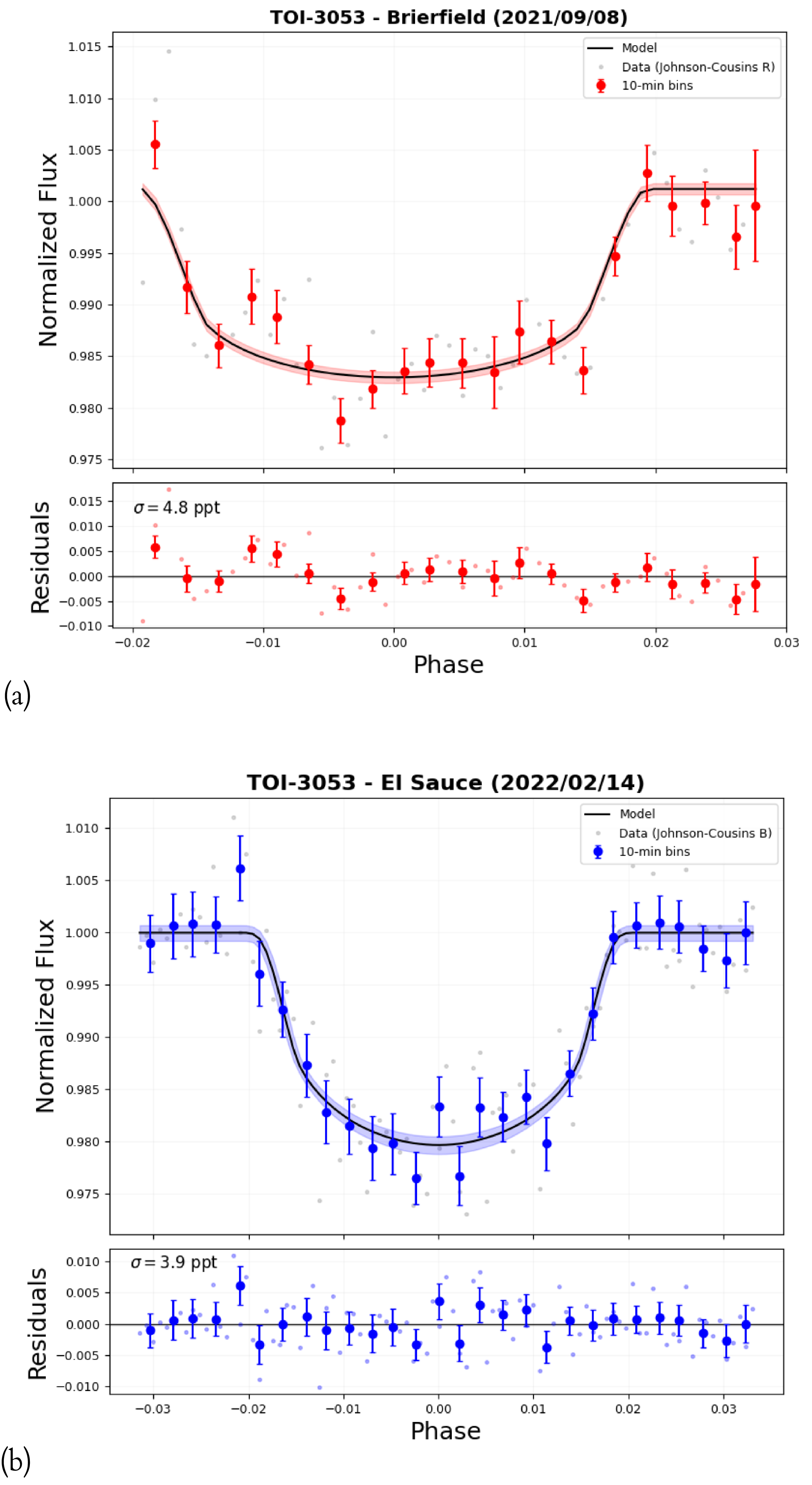
(TFOP SG1, Collins Reference Collins2019). One full transit was observed on 2021/09/08 using the 0.36 m telescope at Brierfield Observatory near Bowral, NSW in Australia. Images were acquired in a Johnson-Cousins R filter with exposures of 240 s using a 4 096
 $\times$
4 096 Moravian 16803 camera (
 $2 \times 2$
binning, 1.47 arsec pix
 $^{-1}$
). Another full transit was observed on 2022/02/14 using the Evans 0.51m telescope at El Sauce Observatory in Coquimbo Province, Chile. 93 images were obtained with a
 $1\,536 \times 1\,024$
STT 1603-3 CCD camera (
 $2\times 2$
binning, 1.08 arsec pix
 $^{-1}$
) using exposures of 180 s in the Johnson-Cousins B filter. Photometric data from these two sessions were extracted using AstroImageJ (Collins et al. Reference Collins, Kielkopf, Stassun and Hessman2017).
2.1.2. TIC 388280249 – TOI-3272
TIC 388280249 is a
 $V \approx 14.2$
mag star in the constellation of Octans. It was observed by TESS in Sectors 11, 12, 13, 27, 38, 39, 65, 66, 67, 93 and 94 at cadences from 1 800 to 200 s. The candidate transit signal (TOI-3272.01) was identified by the Faint Star Search, with an estimated period of 3.147 days and depth of 7.4 ppt. For this target, we use the light curves extracted with the TGLC package. We identify strong photometric variability in all sectors, which is discussed in further detail in Section 3.4.
TOI-3272 was observed by the H50 telescope on three occasions. On the first night (2024/10/02), observations were taken in the SDSS
 $r^{\prime}$
filter with exposures of 120 s. We aquired 75 images, covering the ingress, egress, and post-transit baseline. The conditions were clear with low wind. For the second night (2025/03/24), 84 images were obtained in the Bessell V filter with exposures of 120 s. These data covered the same transit phases as the previous observation of the target. The conditions were clear with low winds again, but the sky background was increased due to an aurora during the observations. Finally, a partial transit in the SDSS
 $i^{\prime}$
filter was captured on 2025/08/19, covering the mid-transit, egress and post-transit baseline. Guiding was sub-optimal for this session due to an issue with the mount, resulting in elongation of the point spread function (PSF) in these images and an increase in photometric scatter.
2.1.3. TIC 304130406 – TOI-3278/HATS-78
TIC 304130406 is a
 $V \approx 14.2$
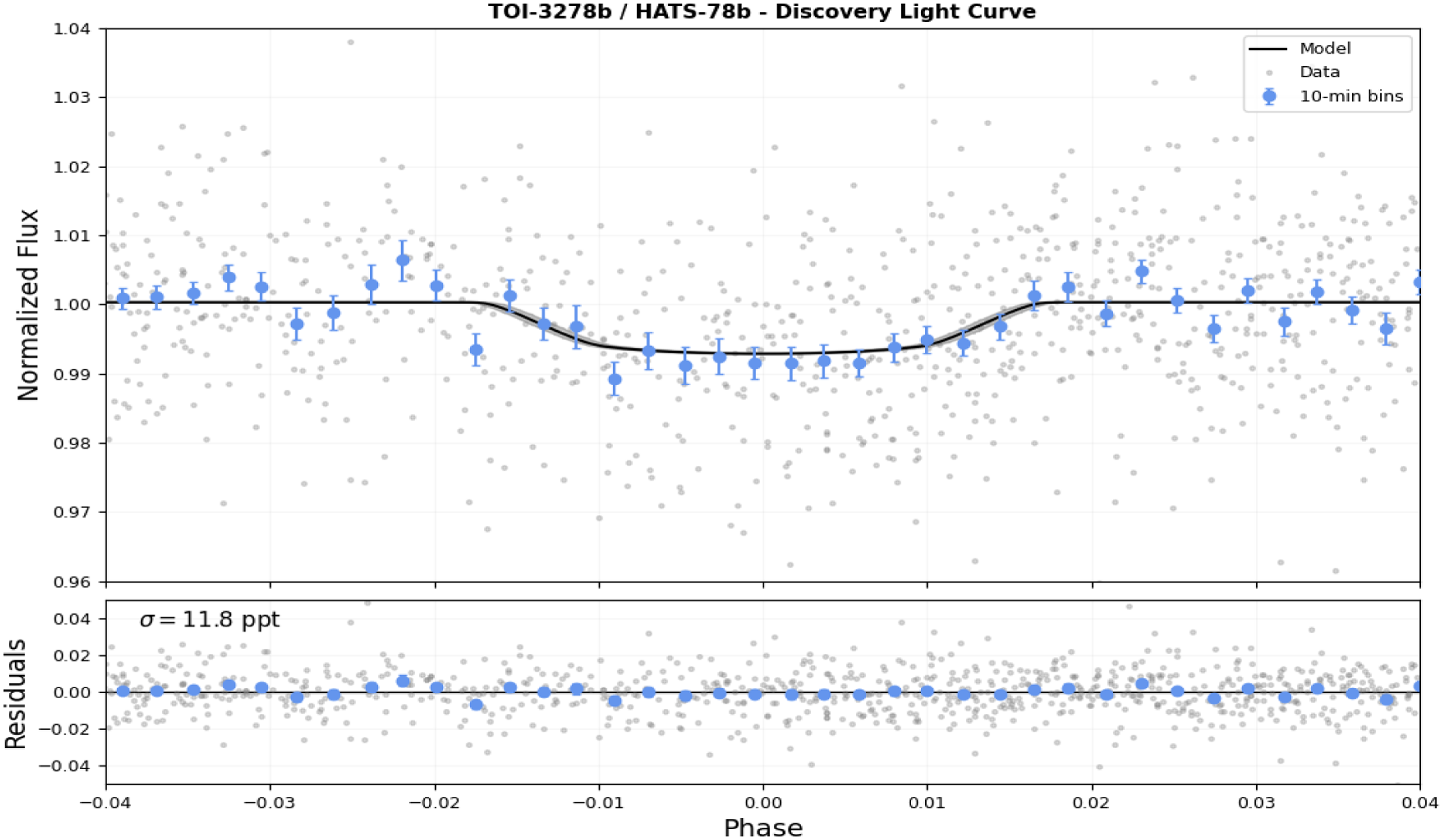
mag star in the constellation of Pavo. It was observed by TESS in Sectors 13, 27, 67 and 94 with cadences of 1 800 to 200 s. TOI-3278.01 was announced by the Faint Star Search, with a candidate signal at 3.25 days and a depth of 8.4 ppt. We also used our custom TGLC extracted light curves for this star. This target was also identified as a planet candidate by the HATSouth survey (Bakos et al. Reference Bakos2013) before the launch of TESS, with the discovery light curve shown in the Appendix (Figure A4).
TOI-3278 was first observed with the H50 on the night of 2024/10/09. We obtained 80 images at 120 s exposures in the SDSS
 $r^{\prime}$
filter, covering a small amount of pre-transit baseline, ingress and the start of egress. Conditions were clear with low moon illumination. However, observations were hindered by moderate to strong winds in the second half of the night. The dome was closed early once the safety limit (25 km h
 $^{-1}$
) was reached, resulting in the post-transit baseline being missed. We then reobserved TOI-3278 on 2025/10/27 in the Bessell V filter, covering similar transit phases. However, the airmass was unfavourable (starting at
 $\chi \, \approx$
2.1), resulting in a relatively poor SNR light curve.
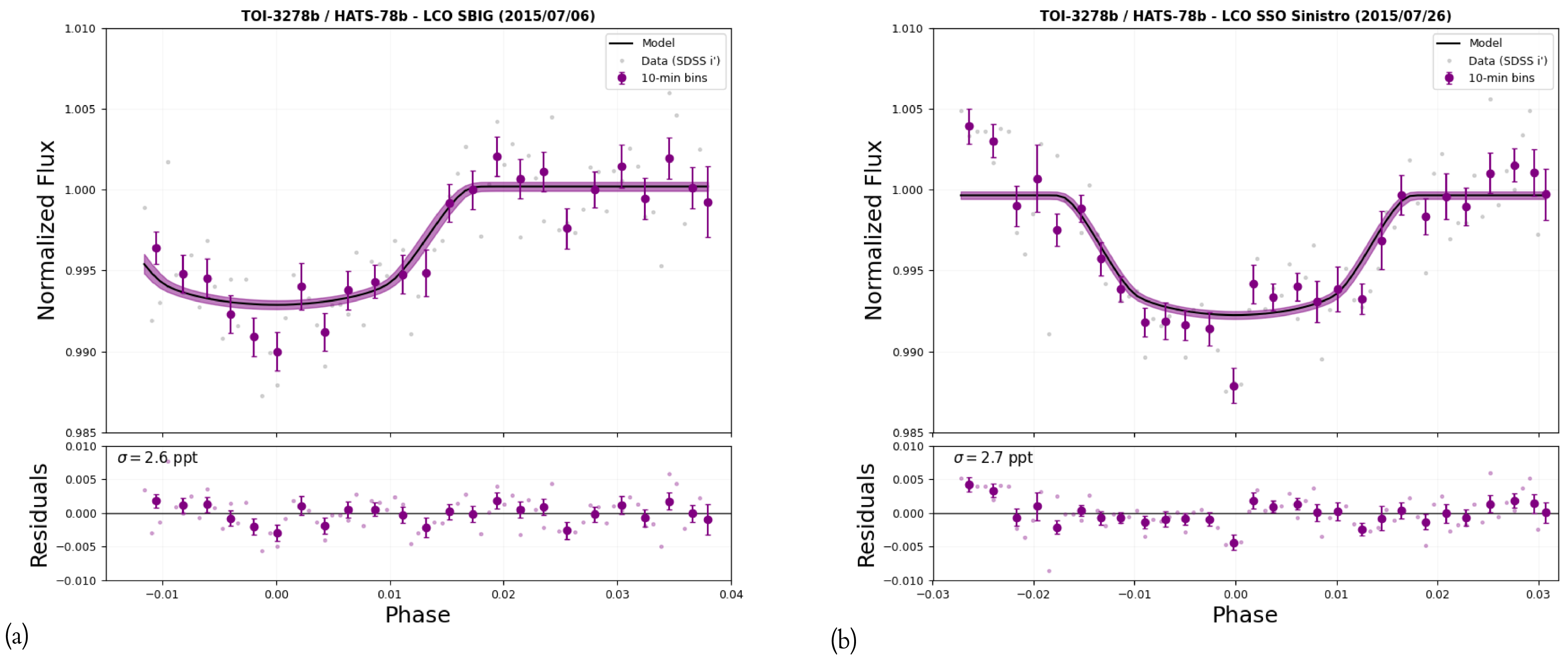
In addition to these light curves, we obtained data from the Las Cumbres Observatory (LCO, Brown et al. Reference Brown2013) telescope network. Two follow-up light curves were obtained by the HATSouth survey on the 1 m telescope at Siding Spring Observatory, Australia (SSO) in 2015. Another light curve was obtained on 2021/06/13 with the 1 m telescope at the Cerro Tololo Inter-American Observatory, Chile (CTIO) through the SG1 program. The images were calibrated with the BANZAI pipeline (McCully et al. Reference McCully, Guzman and Ibsen2018). The CTIO differential photometry was extracted with AstroImageJ using 3.1 arcsec apertures. All LCO data was acquired in the SDSS i
 $^\prime$
filter, using the
 $4\,096\times 4\,096$
SINISTRO camera (0.39 arcsec pix
 $^{-1}$
) or the
 $4\,000 \times 4\,000$
SBIG camera (0.23 arcsec pix
 $^{-1}$
).
2.2. Reconnaissance spectroscopy
To help constrain the stellar atmospheric parameters and attempt to rule out false positive scenarios, such as double-lined eclipsing binaries (EBs), we gathered low to mid resolution spectra for each target. We estimated preliminary spectral types and metallicity values using the PyHammer v2 package (Roulston et al. Reference Roulston, Green and Kesseli2020). Spectral indices and colour regions of input spectra were compared to SDSS templates through a
 $\chi^2$
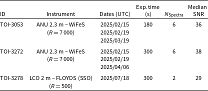
minimisation. This code can also identify some double-lined spectroscopic binaries automatically. The log of the spectroscopic observations is shown in Table 2 and described in further detail here.
Reconnaissance spectroscopy observation logs for TASSIE II TOIs.

Table 2. Long description
The table presents reconnaissance spectroscopy observation logs for TASSIE II TOIs, detailing the instrument used, dates, exposure time, number of spectra, and median signal-to-noise ratio. It has five columns: ID, Instrument, Dates (UTC), Exp. time (s), N Spectra, and Median SNR. The table contains three rows of data. Row 1: ID, TOI-3053; Instrument, ANU 2.3 m – WiFeS (R = 7000); Dates (UTC), 2025/02/15, 2025/02/19, 2025/03/19; Exp. time (s), 180; N Spectra, 6; Median SNR, 36. Row 2: ID, TOI-3272; Instrument, ANU 2.3 m – WiFeS (R = 7000); Dates (UTC), 2025/02/15, 2025/02/19, 2025/04/06; Exp. time (s), 300; N Spectra, 6; Median SNR, 38. Row 3: ID, TOI-3278; Instrument, LCO 2 m – FLOYDS (SSO) (R = 500); Dates (UTC), 2025/07/18; Exp. time (s), 300; N Spectra, 2; Median SNR, 29.
2.2.1. Las Cumbres Observatory – Floyds spectrograph
We obtained two low-resolution (
 $R \approx 500$
) spectra from the Floyds spectrograph on the LCO 2 m telescope at SSO for TOI-3278. The spectra cover wavelength ranges from 320 to 1 000 nm in two orders. We bracketed our science spectra with wire and lamp frames for calibration. Data were reduced by the automatic LCO Floyds pipeline,Footnote
c
which performs order rectification, flat-fielding, and flux calibration. We noticed significant fringing in the infrared (
 $\lambda \gt 750$
nm), so therefore restricted our analysis to the visible part of the spectra. We median combined the two spectra to improve the SNR. We found a mid G-dwarf template star with solar metallicity matches the data well, with no evidence for double lines seen.
2.2.2. ANU 2.3 m – Wide Field Spectrograph (WiFeS)
We obtained mid-resolution (
 $R = 7\,000$
) spectra with the wide field spectrograph (WiFeS) on the Australian National University 2.3 m telescope at SSO (Dopita et al. Reference Dopita2007) for TOI-3053 and TOI-3272. Exposure times ranged between 180 and 300 s depending upon the target, with the aim of obtaining SNR
 $\geq$
30. Ne-Ar arc frames were taken following each observation to ensure an accurate wavelength calibration. Bias, darks, flats, and spectrophotometric standard frames were also collected at the start or end of each night. We utilised the R7000 grating with R560 dichroic, giving a wavelength range of 550–700 nm and velocity resolution of
 $\approx$
45 km s
 $^{-1}$
. Data were reduced using the PyWiFeS package (Childress et al. Reference Childress, Vogt, Nielsen and Sharp2014). Once again, we classified these stars as mid-to-late G-dwarfs.
We also extracted low precision radial velocities (RVs) from the WiFeS data using the iSpec package (Blanco-Cuaresma et al. Reference Blanco-Cuaresma, Soubiran, Heiter and Jofré2014). Each science and standard star spectrum was cross-correlated with an atomic line mask, with the RVs extracted by fitting a 2nd-order polynomial + Gaussian to the peak of cross-correlation function (CCF). The error is calculated from the combination of the target and standard star errors to attempt to account for any zero point drifts. We achieve a precision of
 $\approx$
4 km s
 $^{-1}$
with these data. We ruled out any radial velocity signal greater than 12 km s
 $^{-1}$
, making it unlikely that these targets could be unblended EBs.
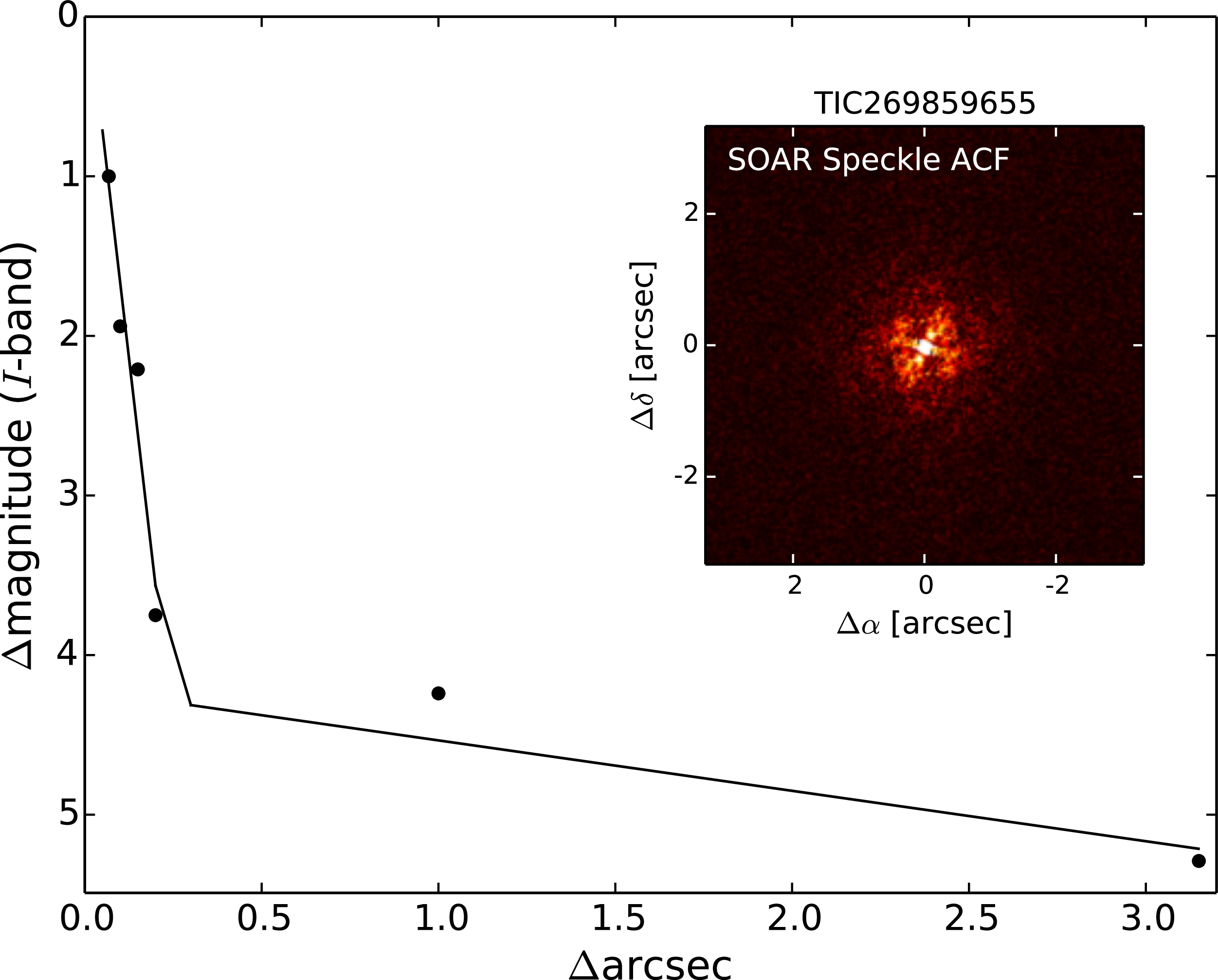
Contrast curve and high-resolution reconstructed autocorrelation function image for TIC269859655 (TOI-3053) from the SOAR telescope with the I filter.

2.3. High angular resolution imaging
To search for close companions, we obtained data from the HRCam Speckle Imager on the Southern Astrophysical Research (SOAR) 4.1 m telescope in I-band (Tokovinin Reference Tokovinin2018) for TOI-3053. This is important to rule out false positives and to correct for any flux dilution of transits, which can lead to underestimation of the planetary radius (Ciardi et al. Reference Ciardi, Beichman, Horch and Howell2015). For details of the data acquisition and reduction, we refer the reader to Ziegler et al. (Reference Ziegler2020). The derived contrast curve and reconstructed auto-correlation function image are shown in Figure 1. We identified no companions to TIC269859655 (TOI-3053) at magnitude differences of
 $\lt$
4 at
 $0.25"$
and
 $\lt$
5 out to 3". Note, we were unable to obtain high angular resolution imaging for the other two targets.
2.4. Radial velocities
2.4.1. CHIRON
We observed TOI-3053 with the CHIRON spectrograph on the 1.5 m telescope operated by the Small and Moderate Aperture Research Telescope System (SMARTS) consortium at CTIO (Tokovinin et al. Reference Tokovinin2013). We utilised the image slicer mode with a spectral resolution of
 $R = 79\,000$
, obtaining 11 observations with exposure times of 3 600 s and bracketed by Th-Ar calibration spectra. The RVs were extracted via least-squares deconvolution of the observed spectra against non-rotating synthetic templates using the ATLAS9 models (Castelli & Kurucz Reference Castelli, Kurucz, Piskunov, Weiss and Gray2003), before fitting a broadening kernel to the final line profile. The median uncertainty on these measurements is 38.5 m s
 $^{-1}$
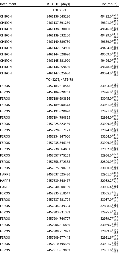
. The RVs are reported in the Appendix (Table A2), with one outlier rejected due to strong moonlight contamination.
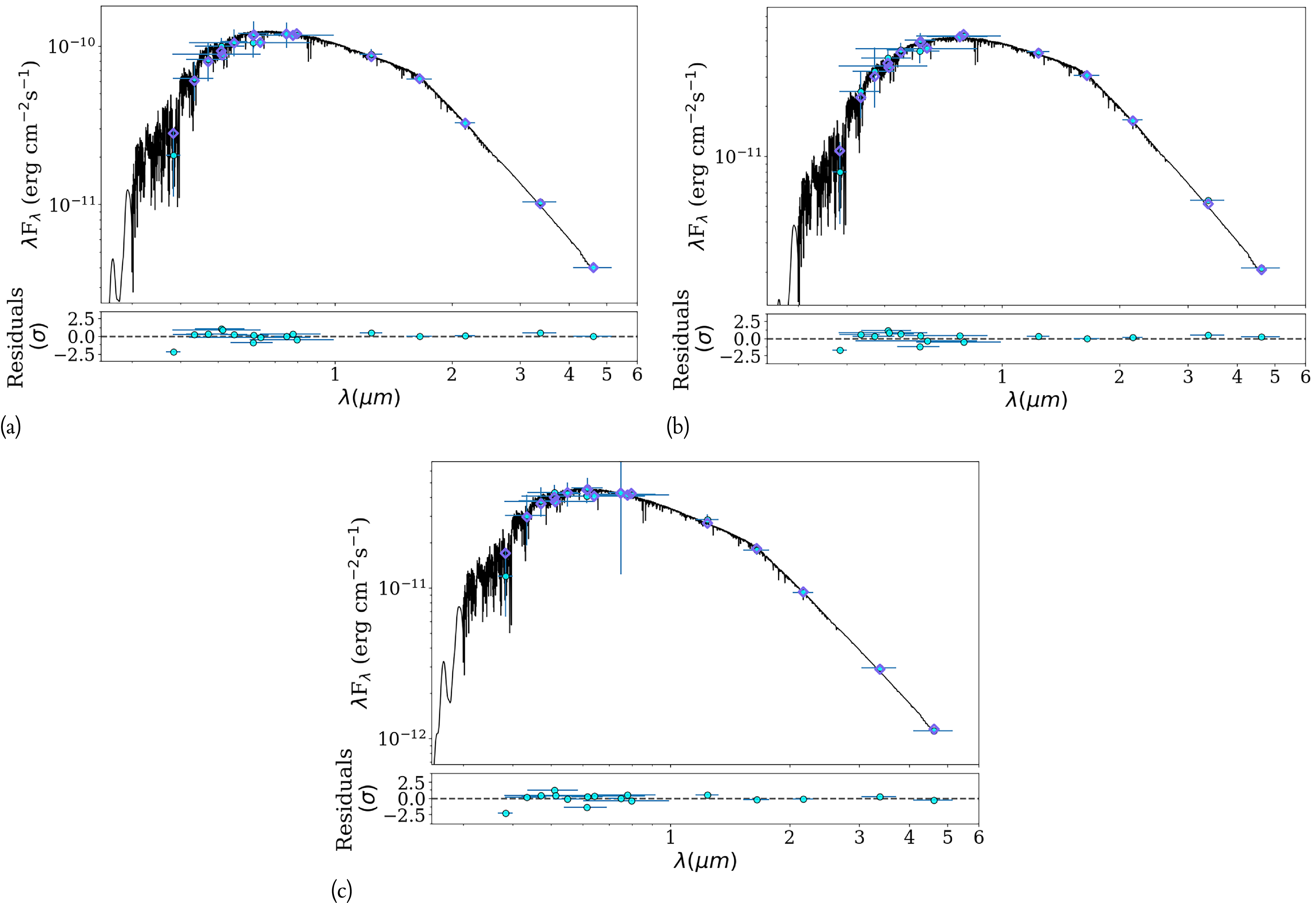
Spectral energy distributions for TOI-3053 (a), TOI-3272 (b), and TOI-3278 (c) from ARIADNE. The best-fit Phoenix v2 models for each star are shown in black, along with the broadband photometry (blue points) and expected flux in each filter (purple diamonds). The residuals are shown in the bottom sub-panel normalised by the uncertainties on each point (in units of standard errors). The horizontal error bars in wavelength represent the bandpass of each filter.

2.4.2. FEROS
We obtained high-resolution spectra of TOI-3278 with the Fiber-fed Extended Range Optical Spectrograph (FEROS, Stahl et al. Reference Stahl, Kaufer, Tubbesing, Guenther, Stecklum and Klose1999) on the MPG/ESO 2.2 m at La Silla Observatory, Chile. FEROS has a spectral resolution of
 $R = 48\,000$
with data split over 39 echelle orders. The radial velocities were extracted using the CERES pipeline with a G2 stellar mask, as described in Brahm et al. (Reference Brahm, Jordán and Espinoza2017). A total of 34 observations were obtained with exposures varying between 1 500 and 3 000 s. Due to the faintness of the target increasing scatter, we decided to clean the data by rejecting 5
 $\sigma$
outliers based on the RVs. This left 24 measurements for modelling, as reported in Table A2. The median uncertainty on these data is 16.5 m s
 $^{-1}$
.
2.4.3. HARPS
We also obtained 3 measurements of TOI-3278 with the High Accuracy Radial velocity Planet Searcher (HARPS, Pepe et al. Reference Pepe, Iye and Moorwood2000) spectrograph on the ESO 3.6 m at La Silla Observatory, Chile. HARPS possesses a spectral resolution of
 $R = 120\,000$
, with data split over 72 echelle orders. The exposure times varied between 1 500 and 1 800 s. The high-precision radial velocities were again extracted with the CERES pipeline using a G2 mask. The median RV error is 27.1 m s
 $^{-1}$
.
3. Stellar characterisation
3.1. Atmospheric parameters
We performed an iterative, multi-step procedure to estimate the stellar atmospheric parameters for each TOI. We started with a spectroscopic analysis using iSpec with the WiFeS spectra. After continuum normalisation (using 2nd order splines) and shifting to rest wavelengths, we median combined the individual spectra to improve the SNR. We selected various metal lines (Fe, Mg, Al, Si, Ca, and Cr), fitting the line centres and profiles using Gaussian functions. We fit for four free parameters (
 $T_{\rm eff}$
, [Fe/H],
 $\log(g)$
,
 $v_{\rm mic}$
) using a grid of pre-computed MARCS model atmospheres (Gustafsson et al. Reference Gustafsson2008). We initially fixed
 $v\sin(i)$
= 2.0 km s
 $^{-1}$
and
 $v_{\rm mac}$
to values from an inbuilt empirical relation, as these parameters are degenerate and not well constrained with the resolution of the WiFeS spectra. For TOI-3278, we were unable to obtain WiFeS spectra and therefore adopted the initial estimates on these parameters from Gaia DR3 XP spectra (as described in Plunkett et al. Reference Plunkett2025).
The spectroscopic estimates were then used as normal priors for spectral energy distribution (SED) fitting with ARIADNE (Vines & Jenkins Reference Vines and Jenkins2022). We collected all available broadband photometric data from surveys such as 2MASS (Skrutskie et al. Reference Skrutskie2006), SkyMapper (Wolf et al. Reference Wolf2018), Gaia DR3 and WISE (Wright et al. Reference Wright2010). We ran nested sampling with four model atmosphere grids, including Phoenix v2 (Husser et al. Reference Husser2013), Kurucz 1993, ATLAS9 (Castelli & Kurucz Reference Castelli, Kurucz, Piskunov, Weiss and Gray2003) and BT-Settl (Allard et al. Reference Allard, Homeier, Freytag, Johns-Krull, Browning and West2011). Two extinction priors were tested, with one using the line-of-sight upper limit from the dust map of Schlafly & Finkbeiner (Reference Schlafly and Finkbeiner2011) (uniform distribution) and the other adopting the Gaia DR3 extinction estimate with a 10
 $\%$
width (normal distribution). Whilst both priors produced consistent values, we decided to use the Gaia DR3 based runs as these led to slightly better fits to the data. The final results were derived from Bayesian model averaging of the individual posterior samples, with the uncertainties estimated from the highest density region at the 68% confidence level. The SEDs are shown in Figure 2 and the derived atmospheric parameters are listed in Table 3. Finally, we attempted to constrain the projected rotational velocity by once again using iSpec. We fixed all other parameters to their previously derived values and fitted broadening kernels to synthetic spectra to match the median combined WiFeS or FEROS data. We were only able to constrain that
 $v\sin(i)$
< 20 km s
 $^{-1}$
for TOI-3053 and TOI-3272. For TOI-3278, we found a tighter constraint of
 $v\sin(i)$
< 2.0 km s
 $^{-1}$
.
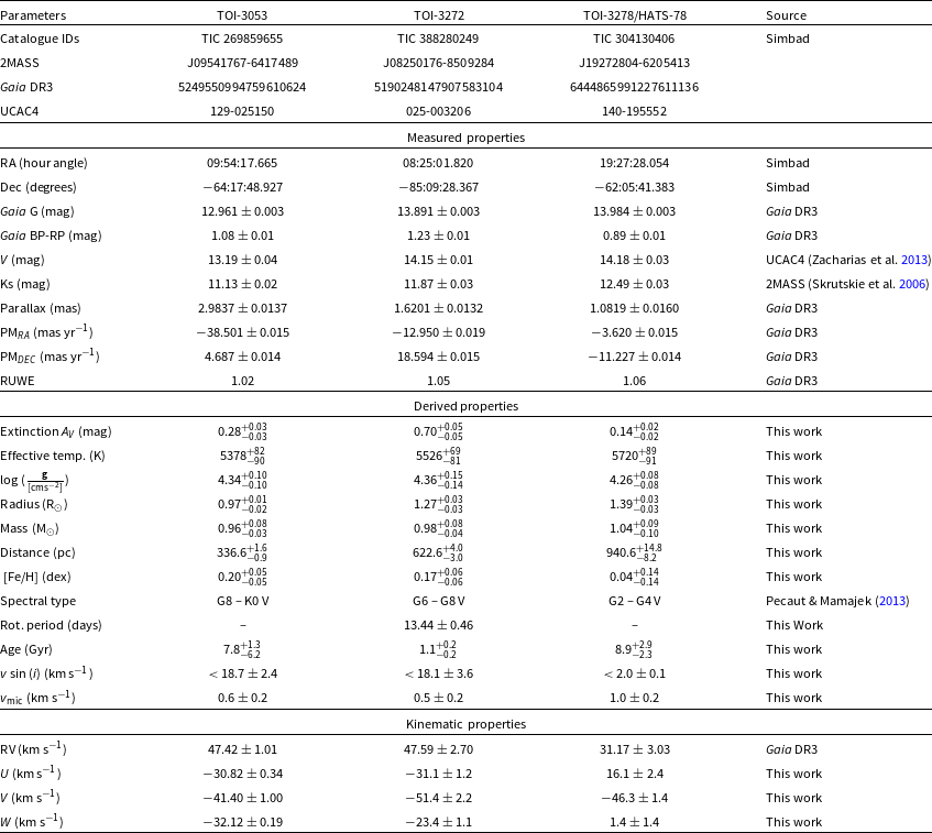
Stellar parameters for TASSIE II TOIs. The reported errors on SED derived parameters account for both statistical and model uncertainties.

Table 3. Long description
The table presents stellar parameters for TOI-3053, TOI-3272, and TOI-3278/HATS-78. It includes catalogue IDs, measured properties such as RA, Dec, Gaia G and BP-RP magnitudes, V and Ks magnitudes, parallax, proper motion in RA and Dec, and RUWE. Derived properties include extinction, effective temperature, surface gravity, radius, mass, distance, metallicity, spectral type, rotation period, age, projected rotational velocity, and microturbulence. Kinematic properties include radial velocity and UVW components. The table has 18 rows and 23 columns, with each column corresponding to a different TOI and each row representing a specific parameter or property.
3.2. Stellar radius and mass
Using the Gaia DR3 parallax as a constraint, ARIADNE estimates the distance and radius of each star by scaling the stellar model fluxes to the observed fluxes. We inferred radii of
 $R_{3053}$
= 0.94
 $\pm$
0.01 R
 $_{\odot}$
,
 $R_{3272}$
= 1.27
 $\pm$
0.03 R
 $_{\odot}$
, and
 $R_{3278}$
= 1.39
 $\pm$
0.03 R
 $_{\odot}$
for TOI-3053, TOI-3272 and TOI-3278, respectively. We then interpolated with MESA isochrones and Stellar Tracks (MIST, Dotter Reference Dotter2016) models to estimate the masses, which are summarised in Table 3. As an independent check of these values, we used the empirical relations of Torres et al. (Reference Torres, Andersen and Giménez2010). These relations were derived from the measured masses and radii of well-detached eclipsing binaries. Using our estimates of
 $T_{\rm eff}$
,
 $\log(g)$
and [Fe/H], we found consistent values for both radius and mass (with larger uncertainties). We adopted the radius and mass estimates from the SED fitting due to the higher precision and consistency with other values.
3.3. Kinematics
We calculated the galactic velocities of each TOI using the equations defined by Johnson & Soderblom (Reference Johnson and Soderblom1987), with an updated transformation matrix for the J2000 epoch. We took the parallax, proper motions and radial velocities in Table 3 from Gaia DR3 (Gaia Collaboration et al. 2023). We adopted the solar velocities of (
 $U_{\odot}, V_{\odot}, W_{\odot}$
) = (8.5, 13.38, 6.49) km s
 $^{-1}$
from Coşkunoğlu et al. (Reference Coşkunoğlu2011). Here, U is defined as positive towards the centre of the galaxy, V is positive in the direction of galactic rotation and W is positive in the direction of the North galactic pole. The results of this analysis are listed in Table 3. Using the membership probabilities defined by Bensby et al. (Reference Bensby, Feltzing and Lundström2003), we placed all targets in the thin disk. We also utilised the BANYAN
 $\Sigma$
tool (Gagné et al. Reference Gagné2018) to check if any of the TOIs are members of known young stellar associations. We found these are likely field stars with 99.9% probability.
3.4. Stellar activity, rotation periods, and ages
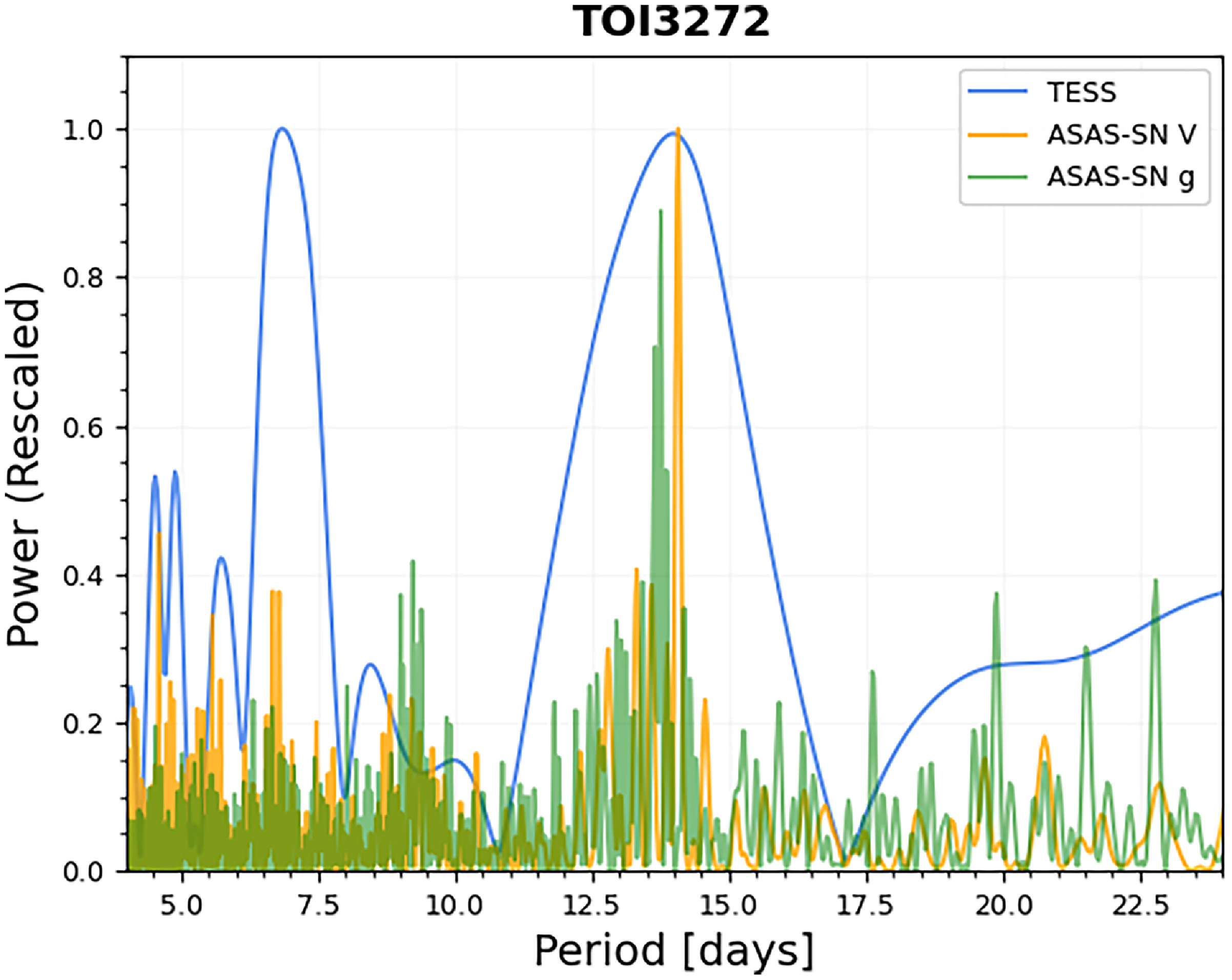
Quasi-periodic variability is seen in the light curve of TOI-3272 at the 1–2% level, consistent with the signatures of star spots. To help constrain the rotational period, we investigated archival photometry from the ASAS-SN (Kochanek et al. Reference Kochanek2017) survey which has a longer observing span than TESS. After cleaning erroneous measurements using sigma clipping (at 5
 $\sigma$
and 10 iterations), we performed a Generalised Lomb-Scargle (GLS) periodogram search (Zechmeister & Kürster Reference Zechmeister and Kürster2009) as shown in Figure 3. We found two peaks at
 $\approx$
6.9 and 13.9 days from TESS data. We determined a similar value of 14.09 days in the ASAS-SN V data, with an alias of 29.95 days in ASAS-SN
 $g^{\prime}$
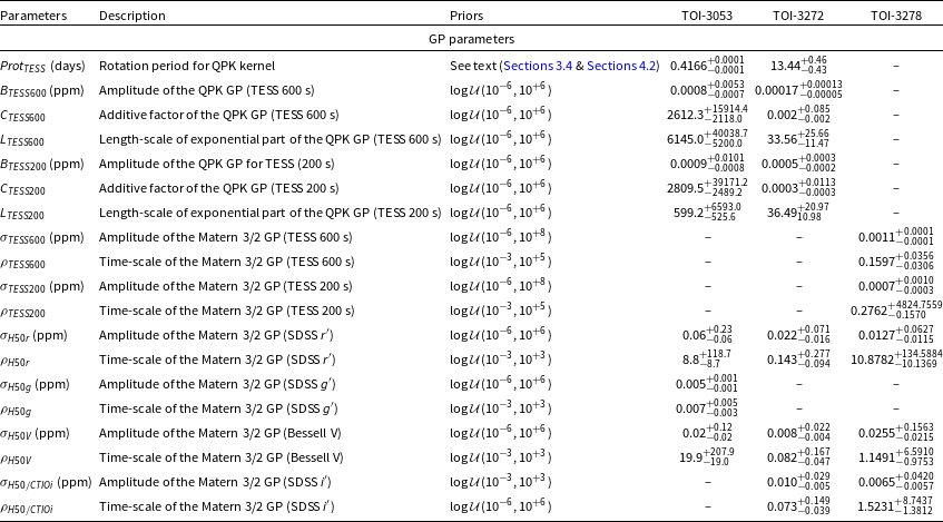
. As a further step in determining which was the true period, we modelled the TESS data with a Gaussian Process through the Celerite package (Foreman-Mackey et al. Reference Foreman-Mackey, Agol, Ambikasaran and Angus2017). We choose a quasi-periodic kernel and provide a broad uniform prior between 5 and 20 days. We recover a consistent estimate of
 $P_{\rm rot}$
=
 $13.44 \pm 0.46$
days and adopt this as the rotational period of TOI-3272. Using the gyrochronology relations of Mamajek & Hillenbrand (Reference Mamajek and Hillenbrand2008) with the known colour of the star, this would imply an age of
 $1.1 \pm 0.2$
Gyr. This places TOI-3272 as a young to intermediate age field star. For TOI-3053 and TOI-3278, we see no clear signs of variability in the TESS or ASAS-SN light curves. This is validated through a GLS search of each dataset returning no matching periods of significance. We also ruled out any periodic signals and RV correlations in the BIS measurements from the FEROS timeseries for TOI-3278. Without rotation periods, we can only place loose age constraints from MIST isochrone fitting (which can have large systematic errors for main-sequence stars). We estimated ages of
 $7.8^{+1.3}_{-6.2}$
and
 $8.9^{+2.9}_{-2.3}$
Gyr for TOI-3053 and TOI-3278/HATS-78, respectively.
4. Data analysis and modelling
4.1. Planet validation
4.1.1. Astrometry
One method for checking for multiplicity in stellar systems is through the Gaia DR3 astrometric solution. In particular, we can look at the renormalised unit weight error (RUWE), which is a weighted chi-square test of the astrometry (accounting for the colour and magnitude of the target). Gaia reports RUWEs of
 $\approx$
1 for each of these targets, which is well below the threshold of 1.4 that usually hints towards unresolved companions (Belokurov et al. Reference Belokurov2020). This helps to rule out eclipsing binaries with scales of 0.1–10 AU as the source of the transit signals.
4.1.2. Archival imaging
To check for background EB scenarios, we investigated archival imaging data from the Harvard College Observatory’s Photographic Glass Plate Collection using the Dasch package (Grindlay et al. Reference Grindlay, Tang, Los, Servillat, Griffin, Hanisch and Seaman2012). We searched data dating back to the late 1890’s for the best image quality and limiting magnitude. We selected frames from between 1930 and 1955 with exposures of 2700 s. By comparing catalogues of sources extracted from stacked H50 images for each target with these earlier epochs, we found no obvious background stars with
 $B \lt 17$
mag. This reduces the likelihood that the transit signals could be caused by background EBs. However, if the relative proper motion of the target and a background star were low enough (below
 $\approx$
10 mas yr
 $^{-1}$
), then it is possible that a background EB could remain blended even after 70 years. The low proper motion of these target stars therefore makes it difficult to completely rule out such a scenario.
Lomb-Scargle periodogram for TIC 388280249 (TOI-3272). The blue curve shows the TESS periods, with the green and orange corresponding to ASAS-SN g and V band periods, respectively. Note, the power for each has been rescaled by dividing by the maximum power value for each dataset.

4.1.3. Transit depth chromaticity
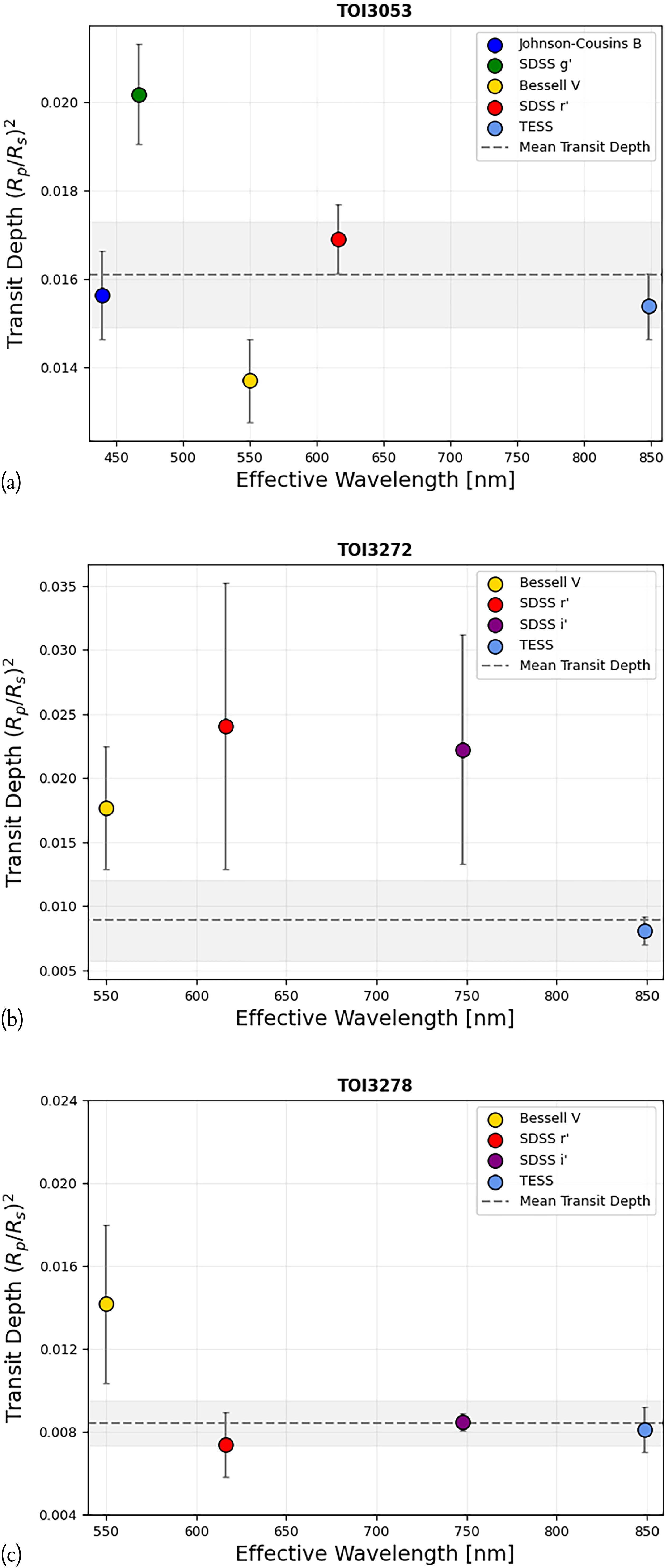
Another method to rule out false positives is to check that the transit depths across different wavelength regions are consistent. We expect planetary transits to be achromatic in broadband filters, with deviation from this condition indicating the signal could be a result of an EB system instead. To check for chromaticity in the transits, we used Juliet (Espinoza et al. Reference Espinoza, Kossakowski and Brahm2019) to fit each light curve from TESS and the ground-based telescopes individually. We applied strict priors on the orbital period, transit epoch and limb darkening coefficients, but allowed the transit depth and impact parameter to explore the full planetary parameter space (with an upper limit of
 $R_{p}/R_{s} \lt 0.2$
). We then extracted the transit depth (by squaring the radius ratio) and compared these against the effective wavelength of each filter used. The results are summarised in Figure 4.
Transit depth as a function of effective wavelength for TOI-3053 (a), TOI-3272 (b) and TOI-3278 (c) from individual fitting with Juliet. The error bars indicate the
 $1\sigma$
range, with the grey dashed line and shaded regions indicating the weighted mean depth and 99.8
 $\%$
confidence interval. The transit appears achromatic for TOI-3053 and TOI-3278, with all points lying within
 $3\sigma$
of the mean (and the TESS value). However, TOI-3272 remains ambiguous due to the large uncertainties.

We can see that TOI-3053.01 and TOI-3278.01 are achromatic, with the transit depths across different filters agreeing within
 $3 \, \sigma$
of the weighted mean (and the TESS value). The minor deviation observed for the SDSS
 $g^{\prime}$
filter with TOI-3053.01 is likely due to poorer data quality from inclement weather. However, the results for TOI-3272.01 remain ambiguous. The depths do not show tight agreement between TESS and the ground-based observations (noting that the wide uncertainties on the H50 measurements means they are statistically consistent). There are two explanations for this. Firstly, as the observations with the H50 do not cover the full transit and have limited baseline coverage, we cannot model for the variability of the star accurately. The spot coverage is changing with each epoch, which is known to alter the measured transit depth if unaccounted for (e.g. Beaulieu et al. Reference Beaulieu, Carey, Ribas and Tinetti2008). Spot modulation should affect shorter wavelength filters more, due to the higher contrast between the cooler starspots and surface in this spectral region. The second possibility is that this is a blended or grazing eclipsing binary system. Given the data, it is difficult to ascertain which scenario is most likely from this test alone.
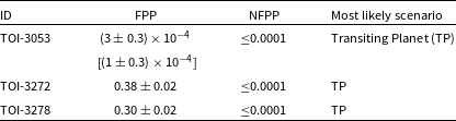
4.1.4. Statistical vetting with TRICERATOPS
To further test for false positive scenarios, we used TRICERATOPS (Giacalone et al. Reference Giacalone2021) with the high cadence (200 s) TESS data and previously derived stellar parameters. The code calculates the false positive probability (FPP) and nearby false positive probability (NFPP) by fitting models for EBs (primary, diluted, background and nearby) and for transits around a primary, secondary or background star. We removed many stars from consideration due to the detection of the transit signals with the H50. Where available, we included the contrast curves from high angular resolution imaging to further constrain the probabilities. We ran 10 iterations of this fitting procedure to ensure consistency in results for each planet candidate. The mean and standard error are reported in Table 4. For TOI-3053.01, TRICERATOPS suggests a very low probability of this being a false positive signal. However, we note that we cannot statistically validate a giant planet with these tests alone because of the overlap in their radius distributions with brown dwarfs and very low mass stars. The FPPs for the other targets suggest that these signals are also likely planetary in nature, but with less certainty. We therefore proceeded to model all the targets further in a global fit.
Vetting results from TRICERATOPS for TASSIE II TOIs. Values in square brackets include the constraint from high angular resolution imaging.

Table 4. Long description
A table comparing false positive probabilities for different TOIs. The table has four rows and four columns. Column headers are ID, FPP, NFPP, and Most likely scenario. Row 1: ID, TOI-3053; FPP, (3 ± 0.3) x 10^-4; NFPP, [1 (± 0.3) x 10^-4]; Most likely scenario, Transiting Planet (TP). Row 2: ID, TOI-3272; FPP, 0.38 ± 0.02; NFPP, ≤0.0001; Most likely scenario, TP. Row 3: ID, TOI-3278; FPP, 0.30 ± 0.02; NFPP, ≤0.0001; Most likely scenario, TP.
4.2. Global modelling with Juliet
We modelled each planetary system with the Juliet package (Espinoza et al. Reference Espinoza, Kossakowski and Brahm2019), which uses the BATMAN transit and RadVel RV fitting codes (Kreidberg Reference Kreidberg2015; Fulton et al. Reference Fulton, Petigura, Blunt and Sinukoff2018). We explore the parameter space via nested sampling as implemented in Dynesty (Speagle Reference Speagle2020), ensuring that the number of live points exceeds the number of parameters squared (i.e.
 $n_{\rm points} \gt n_{\rm param}^2$
). In our modelling, the limb darkening coefficients are re-parameterised following Kipping (Reference Kipping2013), with normal priors set with estimates from the ExoCTK limb darkening calculatorFootnote
d
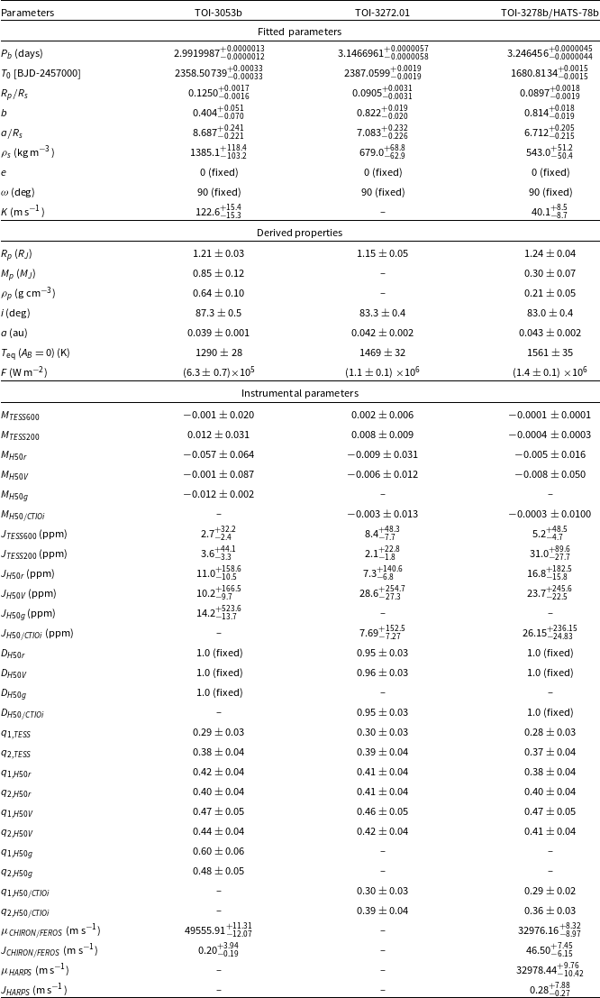
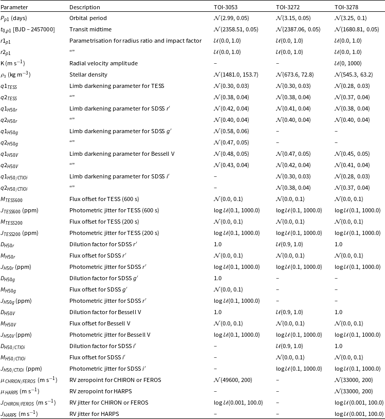
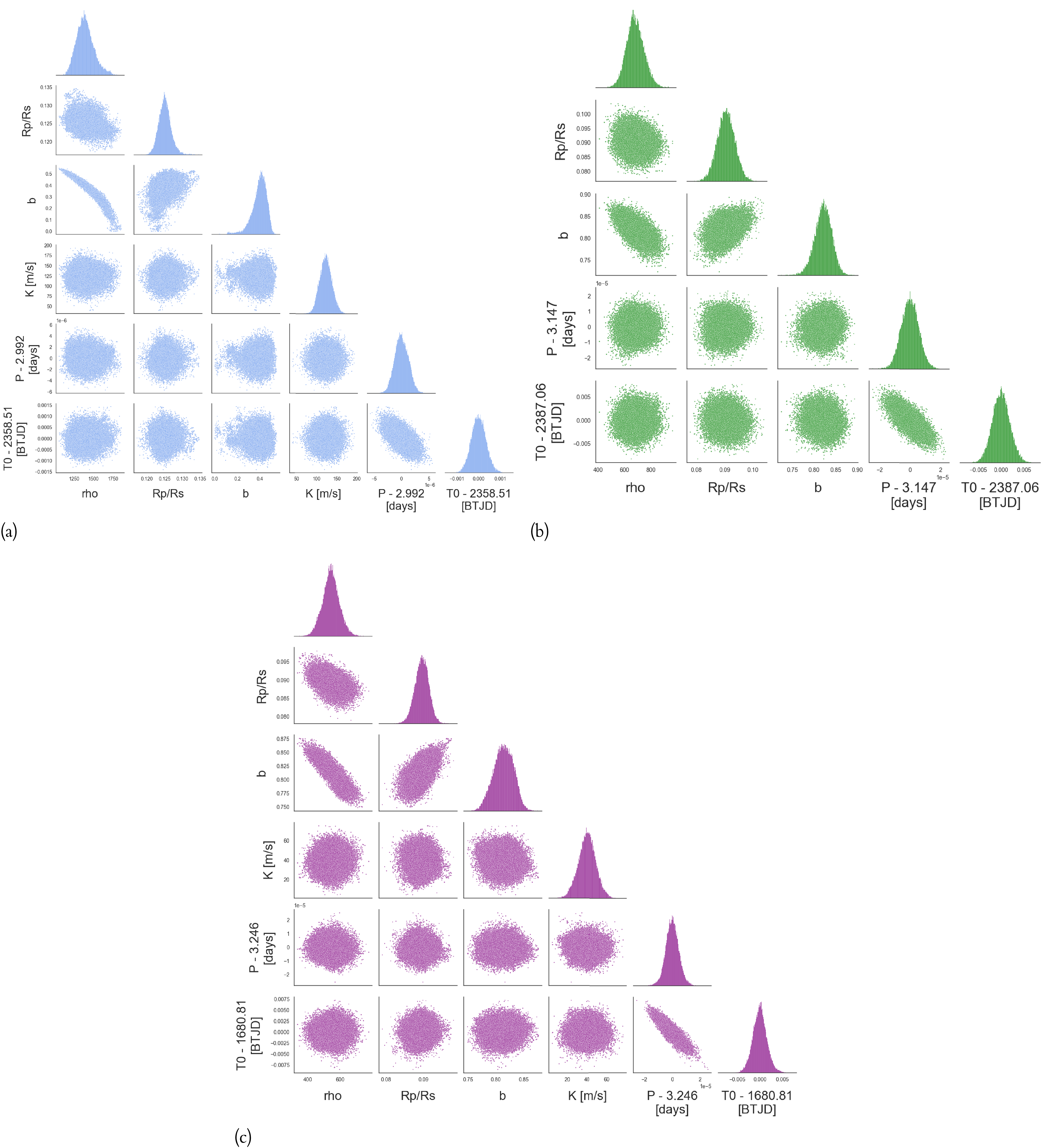
using Phoenix v2 stellar models. The dilution factor for the TESS light curves is set to 1 (no dilution), as they are already de-blended. It was found that only TOI-3272 had non-negligible dilution in the ground-based light curves from a close non-companion star, which we accounted for with a uniform prior with ranges based upon flux ratio estimates from the TRICERATOPS vetting process. We chose to treat each group of cadences from TESS as an individual instrument (i.e. 600 s cadence data are grouped together). This was done to account for different noise levels and systematics from different cadences. The full description of the parameters and priors used in these modelling runs are shown in the Appendix (Tables A3 and A4). We now detail each system individually, with all parameter estimates listed in Table 5 and posterior distributions shown in Figure A10.
4.2.1. TOI-3053
For TOI-3053, we decided to only model data from Sectors 36, 37, 38 and 64 (using the QLP extraction), plus the SDSS
 $r^{\prime}$
, SDSS
 $g^{\prime}$
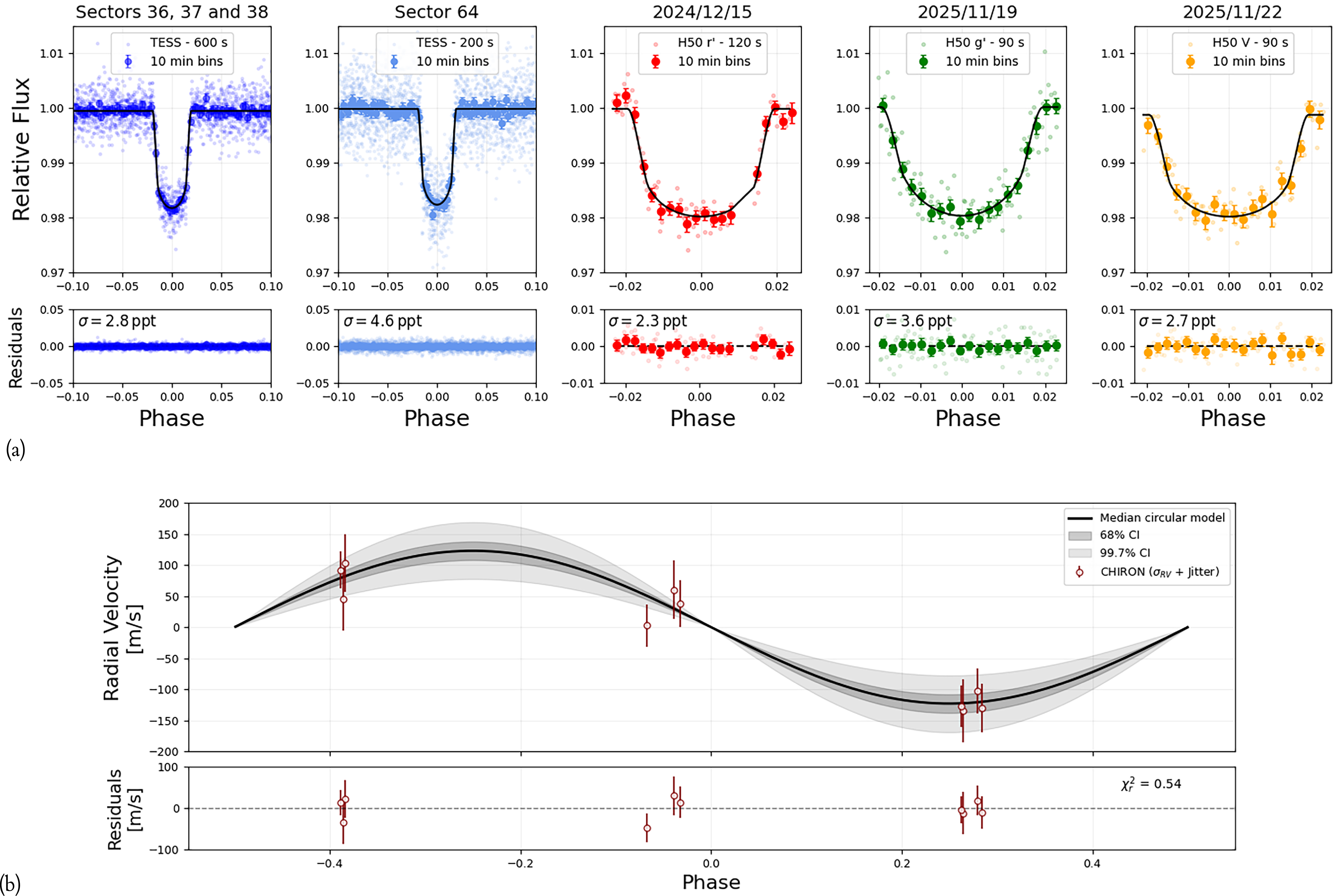
, and Bessell V filters from the H50 and the CHIRON RVs. This was done in the interest of minimising run time while retaining the higher cadence data that had reasonable coverage of the transit profile. We experimented with multiple detrending approaches, in the end favouring two types of GPs: a quasi-periodic kernel (QPK) for TESS and a Matern 3/2 kernel for the H50. We chose the QPK to remove the periodic nuisance signal of the nearby blended eclipsing binary (discussed in Section 2). For the QPK, we set the rotation period hyperparameter to be shared for both TESS instruments and set a normal prior of
 $P_{\rm rot}$
=
 $0.4 \pm 0.1$
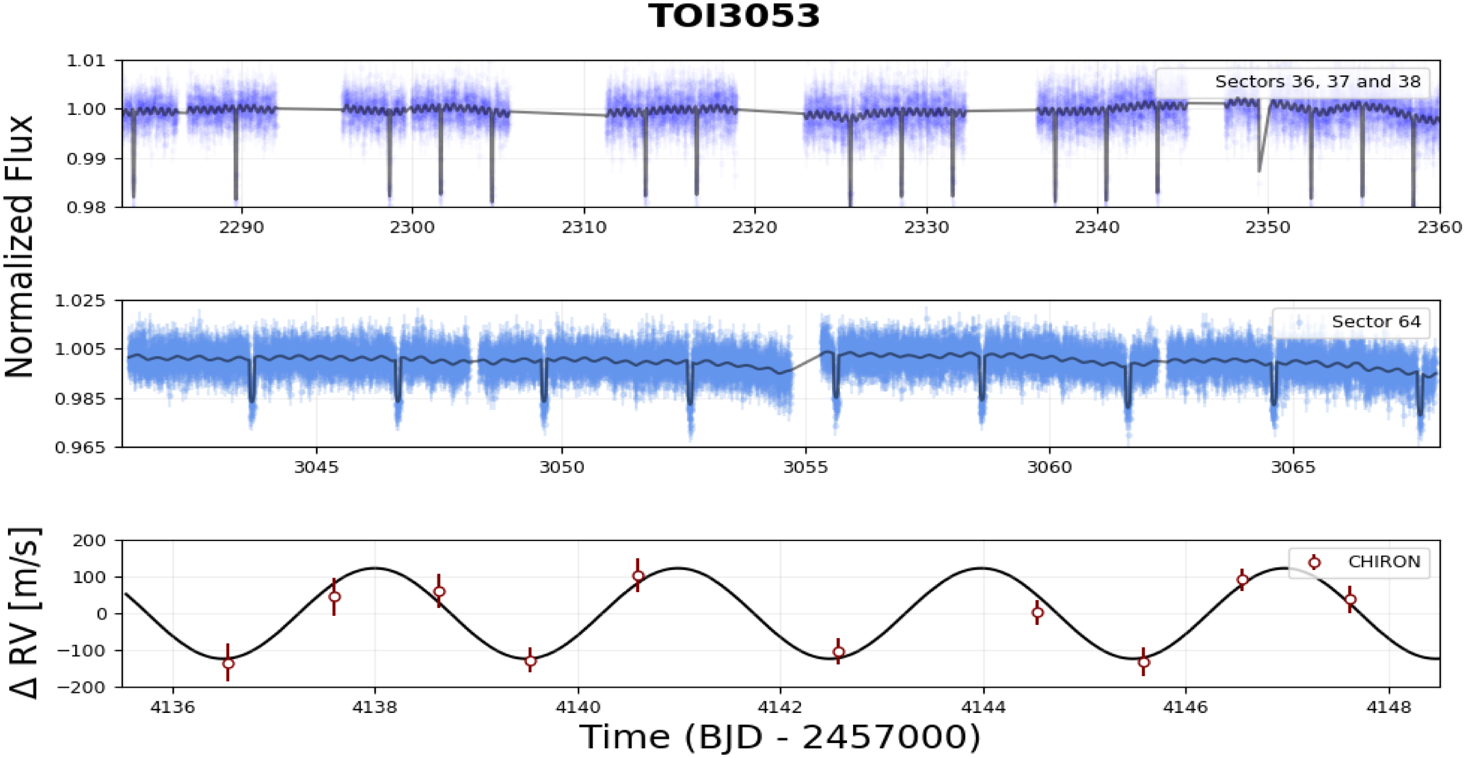
days, based on the period expected from previous BLS periodogram analysis. The phase-folded transit and RVs for each instrument/cadence are shown in Figure 5, with the additional ground-based observations and the multi-sector light curves from TESS displayed in the Appendix (Figures A3 and A6). We find this companion is a hot Jupiter, with
 $R_{3053b}$
=
 $1.21 \pm 0.03$
 $R_{J}$
,
 $M_{3053b}$
=
 $0.85 \pm 0.12$
 $M_{J}$
and a period of
 $P_{3053b}$
=
 $2.9919986 \pm 0.0000012$
days. A circular orbit is preferred (
 $e = 0$
and
 $\omega$
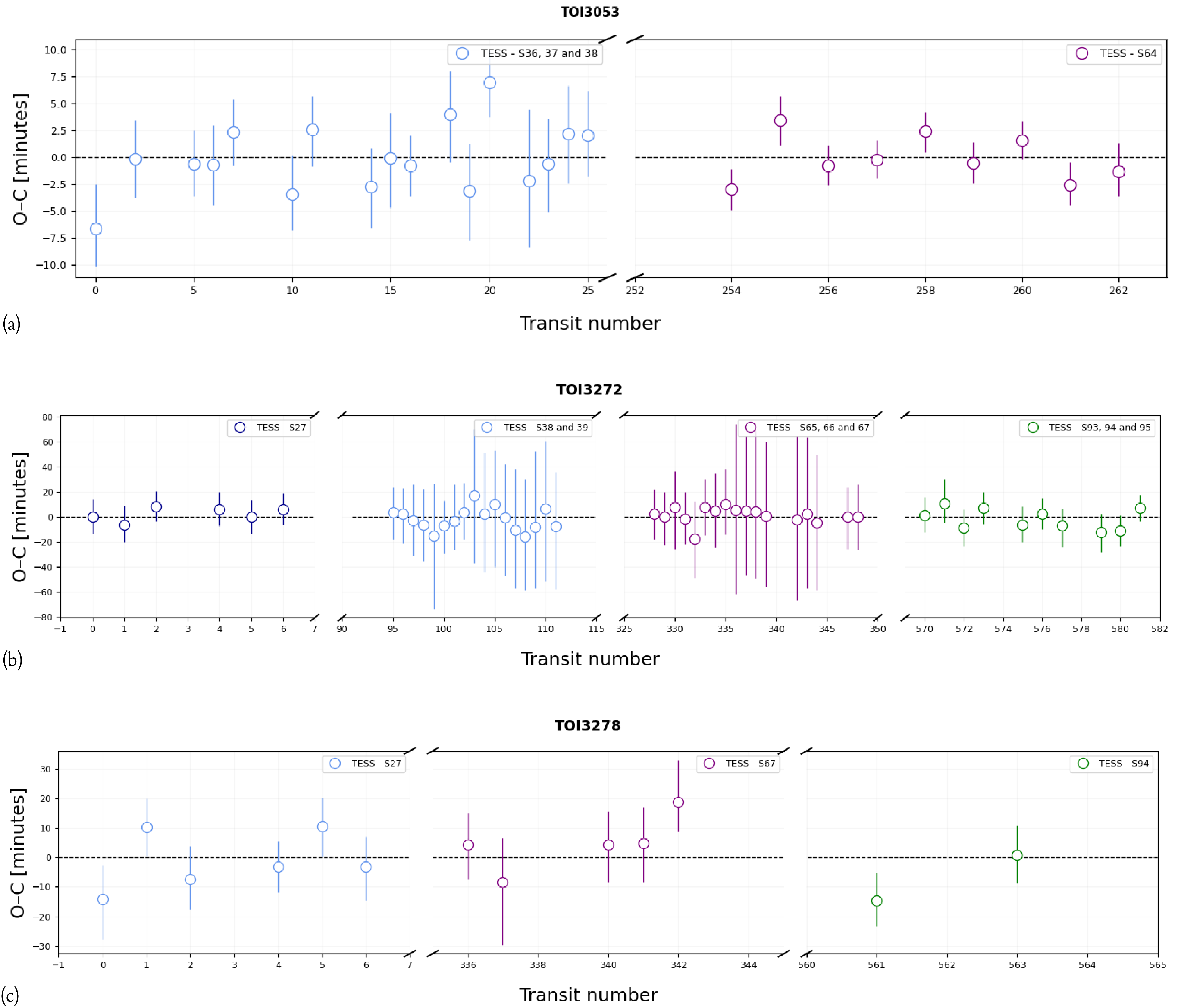
= 90 deg), with the eccentric model having a lower log-likelihood and more parameters. We also ran a fit for transit timing variations (TTVs), fixing all parameters to the best-fit circular model and providing normal priors on each individual transit. We find no evidence for TTVs in this system, with the O-C graph shown in Figure A9(a).
The modelling results from Juliet for the three TASSIE II systems.

Table 5. Long description
Fitted, derived, and instrumental parameters for the three planetary systems TOI-3053b, TOI-3272.01, and TOI-3278b/HATS-78b. Fitted parameters include orbital period, transit epoch, planet-to-star radius ratio, impact parameter, scaled semimajor axis, stellar density, eccentricity, argument of periastron, and radial-velocity semi-amplitude. The orbital periods are approximately 2.999, 3.147, and 3.246 days, respectively. All three eccentricities and arguments of periastron are fixed at zero and 90 degrees, respectively. Derived properties include planetary radius, mass, density, orbital inclination, semimajor axis, equilibrium temperature, and incident flux. The planetary radii are 1.21 ± 0.03, 1.15 ± 0.05, and 1.24 ± 0.04 Jupiter radii, while the masses are 0.85 ± 0.12 and 0.30 ± 0.07 Jupiter masses for TOI-3053b and TOI-3278b/HATS-78b; the mass of TOI-3272.01 is not reported. Equilibrium temperatures are 1290 ± 28, 1469 ± 32, and 1561 ± 35 K, respectively. The instrumental-parameter section gives photometric offsets, jitter terms, dilution factors, limb-darkening coefficients, and radial-velocity parameters for the TESS, H50r, H50V, H50g, H50/CTIOi, CHIRON/FEROS, and HARPS datasets. Some parameters are fixed or unavailable for particular systems, indicated by “fixed” or dashes. Uncertainties are reported at the 1-sigma level.
The phase-folded light curves and RVs for TOI-3053b for each instrument/cadence. In (a), the best-fit transit model is displayed after the subtraction of the GP model for each instrument. The coloured points with error bars represent the photometric data binned to 10-min for clarity. The panels below each light curve show the residuals and measured photometric scatter. In (b), the CHIRON RVs (maroon points) and the best-fit circular model (solid black line) are shown. The light and dark shaded region shows the
 $1\sigma$
and
 $3\sigma$
confidence intervals, respectively.

4.2.2. TOI-3272
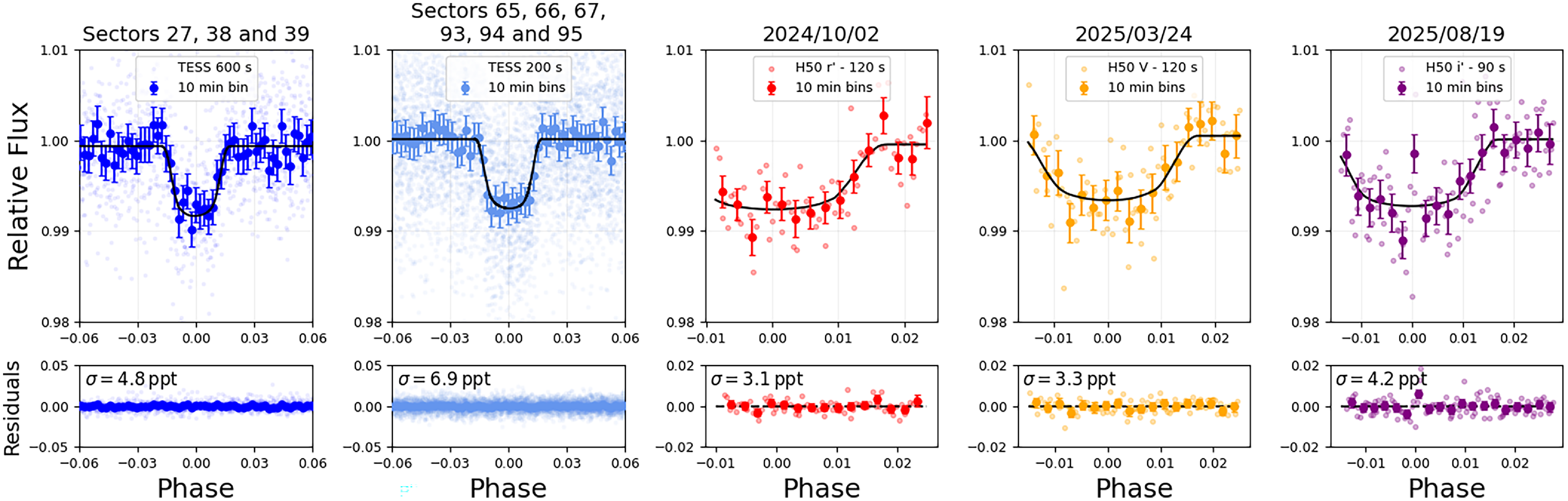
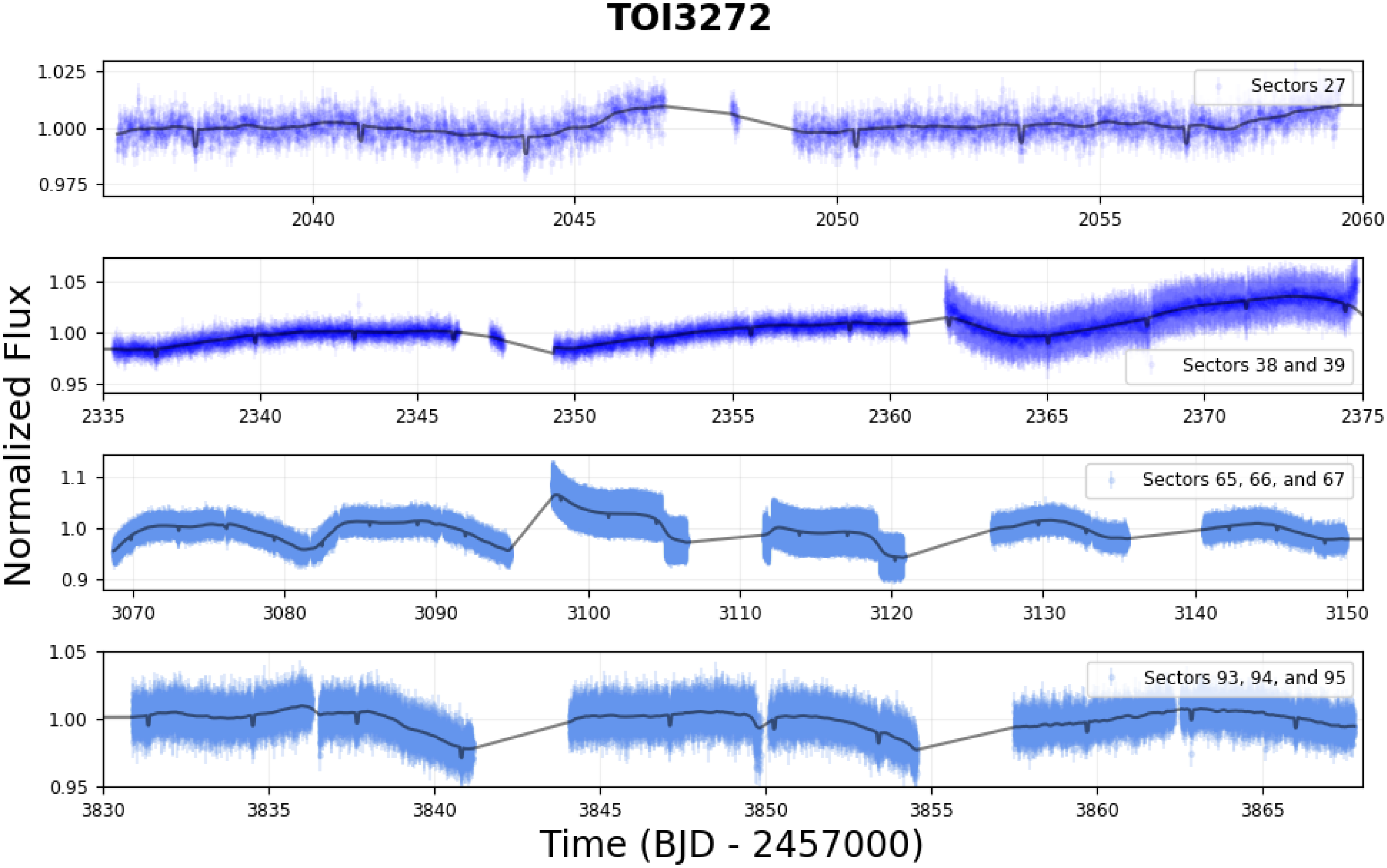
We modelled the data from TESS Sectors 27, 38, 39, 65, 66, 67, 93, 94, and 95, along with all of the H50 light curves for TOI-3272. We chose to again use a QPK kernel on TESS to account for the stellar activity signal, with a 3/2 Matern kernel for the H50. We show the detrended, phase-folded transits in Figure 6 and the full TESS light curves with best-fit transit + GP model in the Appendix (Figure A7). We find a companion with
 $R_{3272.01} = 1.15 \pm 0.05$
and a period of
 $P_{3272.01} = 3.1466961 \pm 0.0000057$
days. A circular orbit is once again preferred and no TTVs were detected. However, the stellar activity combined with the relative faintness of the target resulted in large timing uncertainties (
 $\gt$
30 min) in some TESS sectors, as shown in Figure A9(b). It is important to also note that the posterior distributions of the radius ratio and impact parameter display no severe degeneracies or bi-modalities. This indicates that this system is likely planetary in nature, despite the initial ambiguity in transit depths from individual fitting. Nevertheless, high-precision RVs will be required to confirm the target is in the planetary-mass regime.
The phase-folded light curves for TOI-3272.01 for each cadence/instrument with best-fit transit model (in black), after the subtraction of the median GP model for each instrument. The coloured points with error bars represent the photometric data binned to 10-min for clarity. The panels below each light curve show the residuals and measured photometric scatter.

4.2.3. TOI-3278/HATS-78
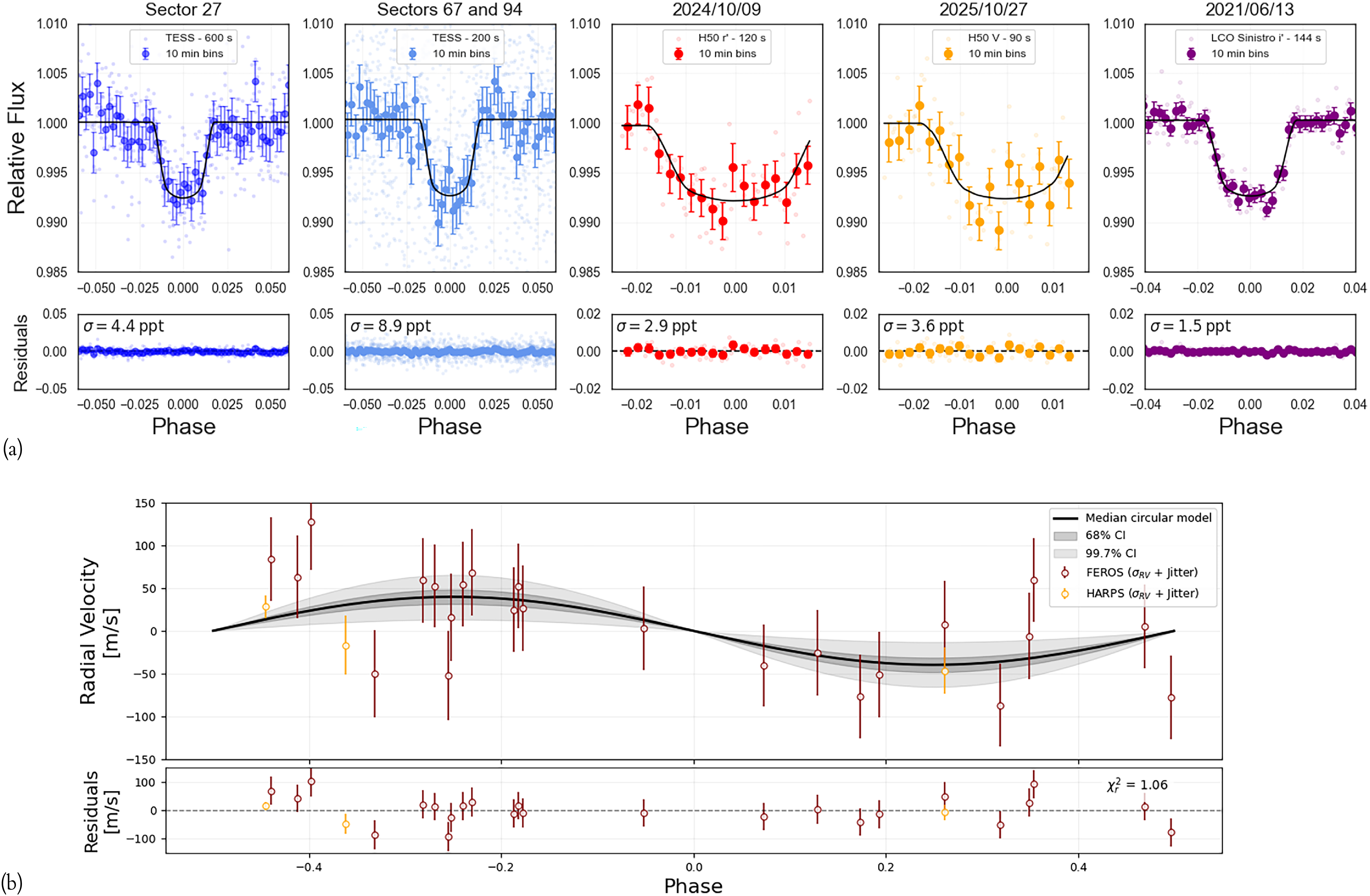
For TOI-3278, the final modelling run was performed with the photometry from TESS Sectors 27, 67, 94 (using the TGLC extraction), two H50 light curves and the LCO CTIO light curve, along with the FEROS and HARPS RVs. Whilst we initially included Sector 13 as well, we discovered that the noise/systematics were too severe to provide meaningful information about the transit and we therefore discarded these data to avoid biasing the fit. We applied a Matern 3/2 GP to the TESS, H50 and CTIO light curves, as there was no indication of periodic stellar activity from the previous periodogram analysis. We explored both circular and eccentric models, finding the circular model was preferred (
 $\Delta\ln Z = 2.03$
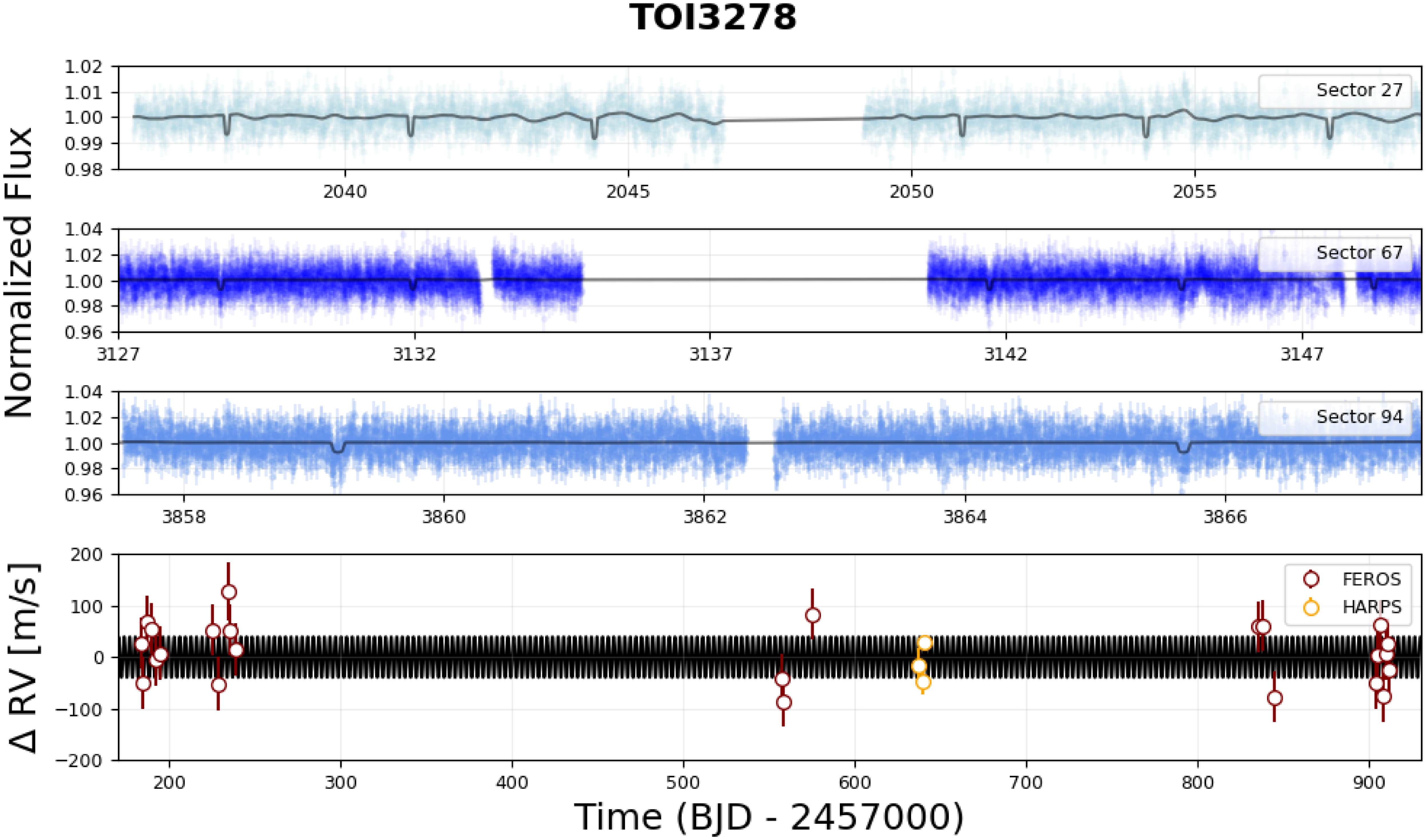
). The phase-folded transits and RVs are shown in Figure 7. The multi-sector TESS light curves and RV timeseries with best-fit transit + RV model, along with the two additional LCO light curves, are shown in the Appendix (Figures A5 and A8). We confirm that TOI-3278 is orbited by an inflated Saturn-mass planet, with
 $R_{3278b}$
= 1.24
 $\pm$
0.04
 $R_{J}$
,
 $M_{3278b}$
= 0.30
 $\pm$
0.07
 $M_{J}$
and
 $P_{3278b}$
= 3.246456
 $\pm$
0.000005 days. Adopting the best-fit circular model parameters, we searched for TTVs and found no evidence for signals above 10 min. This is shown in Figure A9(c).
The phase-folded light curves and RVs for TOI-3278b/HATS-78b for each instrument/cadence. In (a), the best-fit transit model is displayed after the subtraction of the GP model for each instrument. The coloured points with error bars represent the photometric data binned to 10-min for clarity. The panels below each light curve show the residuals and measured photometric scatter. In (b), the RVs are coloured by spectrograph with the best-fit circular Keplerian RV model shown by the solid black line. The light and dark shaded region shows the
 $1\sigma$
and
 $3\sigma$
confidence intervals, respectively.

5. Discussion
5.1. TASSIE II TOIs and the short-period planet population
We now consider the TASSIE II systems in context of the broader short-period planet population.Footnote
e
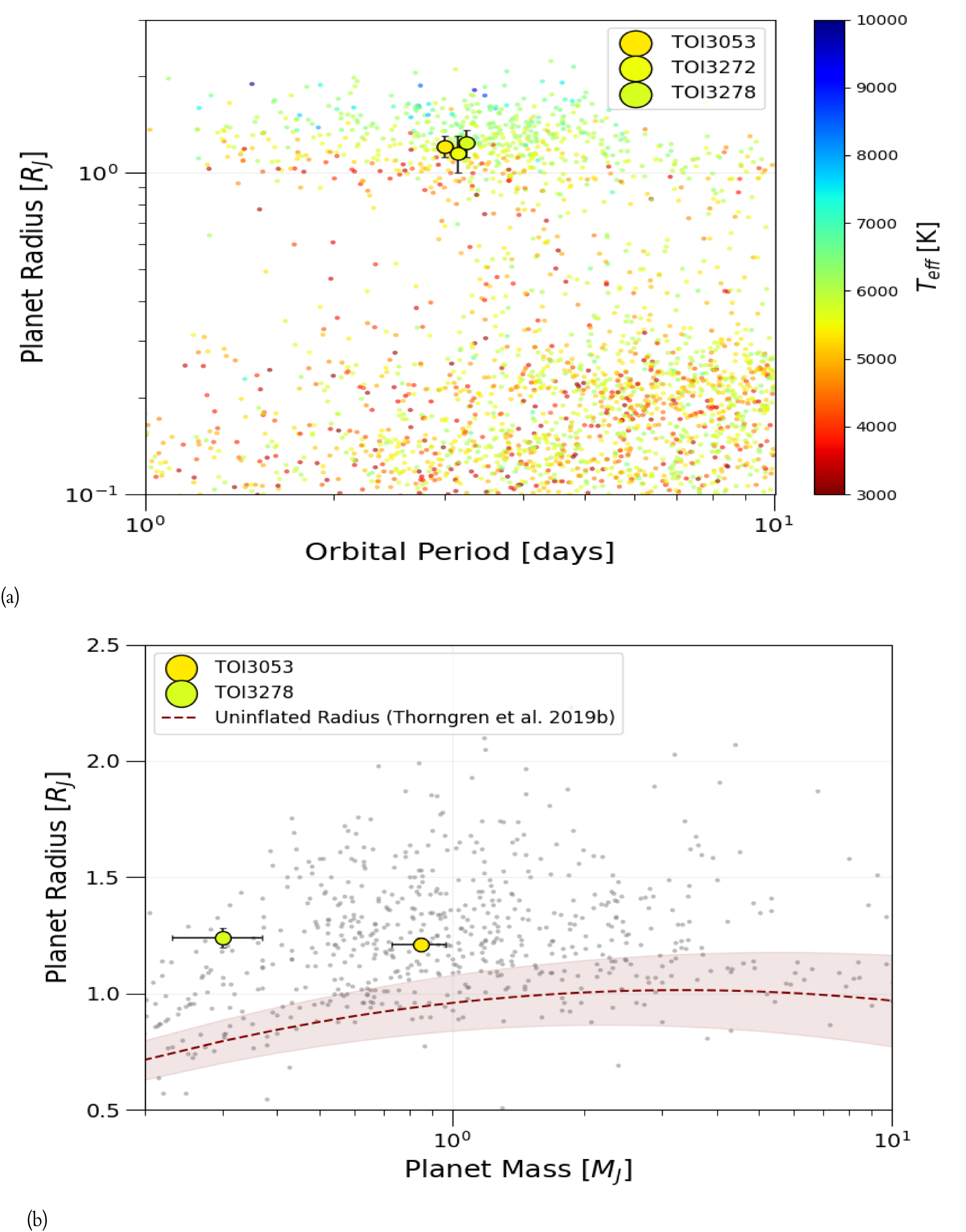
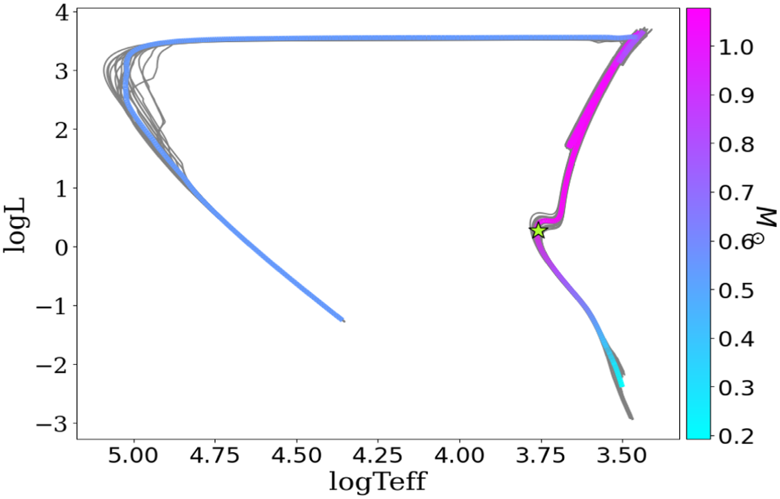
As shown in Figure 8(a), TOI-3272.01 appears consistent with being a HJ based on the position in the radius-period parameter space at the well-known ‘three day pile-up’, sitting with the other two planets studied in this work. For TOI-3053b and TOI-3278b/HATS-78b, we can gain further insights by comparing the measured radii with expectations from empirical mass-radius relations. We can see from Figure 8(b) that both TOI-3053b and TOI-3278b/HATS-78b appear to be inflated, sitting above the uninflated radius line from Thorngren et al. (Reference Thorngren, Marley and Fortney2019). This relation was derived from a sample of ‘warm/cool’ giants (with orbital periods greater than 10 days), including those from the Solar System. It has long been noted that most HJs are inflated, with a correlation between the radius anomaly and incident flux (e.g. Weiss et al. Reference Weiss2013). A universal explanation for radius inflation remains elusive, but mechanisms such as ohmic heating or thermal tides have been shown to each match certain features of the observed HJ population (see Sarkis et al. Reference Sarkis, Mordasini, Henning, Marleau and Mollière2021). A larger sample of hot giant planets, especially around young and post-main sequence stars, will be required to determine which mechanism is the predominant avenue of inflation. Interestingly, the inferred age of TOI-3278 implies that is is close to the end of its main-sequence lifetime (
 $\approx$
9–10 Gyr). The proximity of the star to the main-sequence turn-off in the Hertzsprung-Russell diagram from SED + MIST isochrone fitting is consistent with this scenario (as shown in Figure A2). This would imply that TOI-3278b/HATS-78b may be undergoing a period of re-inflation, as the expansion of its host star increases the irradiation of the planet. This makes the system an intriguing target for further study.
The mass-radius-period parameter spaces for short-period exoplanets. In (a), the radii and orbital periods of known planets are shown with systems coloured by the stellar effective temperature. The TASSIE II TOIs are highlighted as points with
 $3\sigma$
error bars for their radii. In (b), the radii and masses are shown for known HJs. TOI-3053b and TOI-3278b/HATS-78b are shown with error bars representing the
 $1\sigma$
errors on mass. The dashed line and shaded regions show the predicted uninflated radius as a function of mass using the relation from Thorngren et al. (Reference Thorngren, Marley and Fortney2019). Data from the NASA Exoplanet Archive.

5.2. Future observations and atmospheric characterisation
Whilst we were able to confirm TOI-3053b and TOI-3278b/HATS-78b as planetary in nature, TOI-3272.01 remains as a candidate despite passing various false positive tests. The RV signal from TOI-3272 will likely be more challenging to characterise, due to the presence of spots/activity and the host star being relatively faint. Confirming that TOI-3272 is indeed a young star will be an important first step to decide if RV observations should be attempted, with a single high-resolution spectrum targeting typical youth indicators (e.g. Ca H & K line emission or Li non-depletion) being recommended. If this target is indeed a giant planet orbiting a young field star, this could be an important addition to our understanding of giant planet evolution through the first billion years of a system’s life. High angular resolution imaging of TOI-3272 and TOI-3278 would also be beneficial to firmly rule out any stellar companions below the Gaia detection limit that may contaminate photometry and influence the radius and age estimates.
We also assessed each target’s suitability for atmospheric measurements with JWST or Ariel. We found that the targets are generally too faint to perform transmission spectroscopy with either instrument, with some caveats. For TOI-3053b and TOI-3278b/HATS-78b, we calculate the transmission spectroscopy metric (TSM) following Kempton et al. (Reference Kempton2018) and find
 $TSM_{3053} = 70 \pm 12$
and
 $TSM_{3278} = 71 \pm 18$
using our previously derived parameters. For TOI-3272.01 which does not have a mass measurement, we assume a fiducial mass of 1
 $M_{J}$
and estimate a TSM of 24. These all fall below the recommended threshold of
 $TSM \gt 90$
for giant planets (Kempton et al. Reference Kempton2018). However, if the mass of either is closer to their lower confidence interval bounds, then the planets will pass this threshold and become possible targets for transmission spectroscopy with JWST. Regardless, the low density and possible re-inflation of TOI-3278b/HATS-78b may still justify investigation with JWST phase curves to map the temperature profile of the planet and look for signatures of atmospheric escape (e.g. through infrared metastable He absorption, see Krishnamurthy et al. Reference Krishnamurthy2026). Furthermore, the upcoming release of Gaia DR4 epoch astrometry presents an exciting opportunity to search for long-period outer companions to these systems, as expected from a HEM migration channel (e.g. Lammers & Winn Reference Lammers and Winn2026).
6. Conclusion
In this paper, we have studied three close-in giant transiting exoplanet candidates alerted by TESS that are orbiting Sun-like stars. Using ground-based follow-up light curves from the UTGO H50 telescope, along with auxiliary astrometric, imaging and RV data, we were able to confirm TOI-3053b and TOI-3278b/HATS-78b as hot giant planets. TOI-3053b is a typical hot Jupiter, with a radius of
 $R_{3053b}$
= 1.21
 $\pm$
0.03
 $R_{J}$
and mass of
 $M_{3053b}$
= 0.85
 $\pm$
0.12
 $M_{J}$
. TOI-3278b/HATS-78b was found to be a highly inflated Saturn-mass planet (
 $R_{3278b}$
= 1.24
 $\pm$
0.04
 $R_{J}$
,
 $M_{3278b}$
= 0.30
 $\pm$
0.07
 $M_{J}$
) orbiting a potentially old star (T
 $_{3278}$
= 8.9
 $^{+2.9}_{-2.3}$
Gyr) that could be close to the end of the main-sequence lifetime. We also investigated TOI-3272.01 which, despite remaining unconfirmed, is consistent with being a hot Jupiter (with
 $R_{3272.01} = 1.15 \pm 0.05 \, R_{J}$
). TOI-3272 is an exciting target for further study as a potentially young system (T
 $_{3272}$
=
 $1.1 \pm 0.2$
Gyr), which may provide an important constraint for studies of the radius inflation of HJs. Whilst these planets are not ideal targets for atmospheric measurements with JWST or Ariel, future studies using Gaia DR4 epoch astrometry and JWST phase curves remain a viable possibility. Furthermore, these systems add to our sample of companions orbiting relatively faint stars (
 $V \gt 13$
mag) that will be common targets for upcoming space-based transit missions, such as the Nancy Grace Roman Galactic Bulge Time Domain Survey (Akeson et al. Reference Akeson2019). Although these faint and distant host stars present challenges to confirmation efforts (Wilson et al. Reference Wilson2023), they will be vital in understanding the influence of galactic environment on exoplanet formation and evolution.
Acknowledgements
The authors wish to thank both Andrew Vanderburg for his valuable suggestions for the false positive vetting of TOI-3053.02 and Kim McLeod for providing one of the LCO datasets used in this work. We also thank the anonymous reviewer for their comments that helped to improve the manuscript.
Based on observations obtained at the Greenhill Observatory, which is owned and operated by the University of Tasmania. The observatory was made possible by generous donations from Caisey Harlingten and the UTAS Foundation. We acknowledge Palawa, as the original owners of Lutruwita/Tasmania on which the observatory stands.
This work uses data acquired at the Siding Spring Observatory with the Australian National University 2.3 m Telescope. We acknowledge the traditional custodians of the land on which the telescope stands, the Gamilaraay people, and pay our respects to elders past and present.
This paper includes data collected by the TESS mission, which are publicly available from the Mikulski Archive for Space Telescopes (MAST). Funding for the TESS mission is provided by NASA’s Science Mission directorate. We acknowledge the use of public TESS Alert data from pipelines at the TESS Science Office and at the TESS SPOC. Resources supporting this work were provided by the NASA High-End Computing (HEC) Programme through the NASA Advanced Supercomputing (NAS) Division at Ames Research Centre for the production of the SPOC data products.
This work has made use of data from the European Space Agency (ESA) mission Gaia (https://www.cosmos.esa.int/gaia), processed by the Gaia Data Processing and Analysis Consortium (DPAC, https://www.cosmos.esa.int/web/gaia/dpac/consortium). Funding for the DPAC has been provided by national institutions, in particular the institutions participating in the Gaia Multilateral Agreement.
This research has made use of the SIMBAD database and VizieR catalogue access tool, operated at CDS, Strasbourg, France.
This research has made use of NASA’s Astrophysics Data System. This research has made use of the NASA Exoplanet Archive, which is operated by the California Institute of Technology, under contract with the National Aeronautics and Space Administration under the Exoplanet Exploration Programme.
Data availability statement
All light curves and spectra obtained for the TASSIE program will be uploaded to ExoFOP (https://exofop.ipac.caltech.edu/tess/) after publishing. FEROS and HARPS spectra are available through the ESO Science Archive. The analysis notebooks for this work can be viewed here: https://github.com/tjplunkett/TASSIE_II
Author contributions
Conceptualisation: T.P. Methodology: T.P; E.T; J.R.; A.C.; JP.B. Observations/Data Curation: T.P; A.C; J.S; B.E; + remaining authors. Data visualisation: T.P; C.Z. Writing original draft: T.P. All authors approved the final submitted draft.
Funding statement
T.P. is supported by an Australian Government Research Training Program (RTP) Scholarship. E.T. has been supported by the Australian Government through the Australian Research Council Discovery Project Grant 240101842. J.S. was supported in part by funding provided by the National Aeronautics and Space Administration (NASA), under award number 80NSSC20M0124, Michigan Space Grant Consortium (MSGC). K.P. acknowlegdes support from NSF grant 2311527, and NASA grant 80NSSC25K0379. R.B. acknowledges support from Fondecyt Project 1241963. A.J. acknowledges support from Fondecyt project 1251439. Development of the HATSouth project was funded by NSF MRI grant NSF/AST-0723074, operations were supported by NASA grants NNX09AB29G, NNX12AH91H, and NNX17AB61G, and follow-up observations were partially supported from grant NSF/AST-1108686.
Competing interests
The authors are not aware of any competing interests.
Appendix A. Auxiliary figures and tables
The difference image centroid test for the 0.416 day signal in the TOI-3053 light curves. The positions of TOI-3053 and the nearby false positive EB are highlighted with gold and red crosses, respectively. The colour bar indicates the decrease in flux measured in-eclipse (in parts per thousand).

The Hertzsprung-Russell diagram of TOI-3278/HATS-78 from the ARIADNE SED + MIST isochrone fitting. The thick coloured line is the interpolated MIST isochrone corresponding to the best-fit stellar parameters. The colourbar traces the stellar mass for each section of the evolutionary track. The grey lines are 20 random samples drawn from the parameter posterior distribution, showing the uncertainty on the fit. The star icon shows the inferred logarithm of the luminosity and temperature for TOI-3278/HATS-78, with the position close to the main-sequence turn-off.

Additional photometry logs for TASSIE II TOIs.

Table A1. Long description
The table presents observation logs for TASSIE II TOIs using various ground-based telescopes. It includes columns for ID, Dates (UTC), Filter, Exp. time (s), FWHM ("), and Airmass. The table has 11 rows and 6 columns. Row 1: TOI-3053, 2024/12/15, r, 120, 2.6, 84. Row 2: TOI-3053, 2025/02/22, r, 150, 3.2, 37. Row 3: TOI-3053, 2025/03/04, r, 120, 3.0, 61. Row 4: TOI-3053, 2025/11/19, g, 90, 3.4, 110. Row 5: TOI-3053, 2025/11/22, V, 120, 2.2, 85. Row 6: TOI-3053, 2025/12/03, i, 90, 3.4, 120. Row 7: TOI-3272, 2024/10/02, r, 120, 2.2, 75. Row 8: TOI-3272, 2025/03/24, V, 120, 2.0, 84. Row 9: TOI-3272, 2025/08/19, i, 90, 2.1, 112. Row 10: TOI-3278, 2024/10/09, r, 120, 3.1, 80. Row 11: TOI-3278, 2025/10/27, V, 150, 2.4, 70."
Follow-up light curves for TOI-3053b from the Brierfield (a) and El Sauce (b) observatories. The coloured points with error bars show the individual photometric points (in grey) binned to 10-min for clarity. The best-fit transit model from Section 4.2 is overlaid in black. The residuals and photometric scatter are shown in the bottom panels of each plot.

Radial velocities for TOI-3053 and TOI-3278/HATS-78.

Table A2. Long description
Radial-velocity measurements for TOI-3053 and TOI-3278/HATS-78. The table lists the observing instrument, observation time as BJD-TDB in days, and measured radial velocity in metres per second, with asymmetric uncertainties. For TOI-3053, ten measurements were obtained with CHIRON at BJD-TDB 2461136.545220–2461147.625680. The measured radial velocities range from approximately 49429 to 49648 m s⁻¹, with uncertainties of about 30–51 m s⁻¹. For TOI-3278/HATS-78, measurements were obtained primarily with FEROS, with two measurements from HARPS. The FEROS observations span BJD-TDB 2457183.618548–2457911.819862, while the two HARPS measurements were obtained at BJD-TDB 2457637.525480 and 2457639.548477. The TOI-3278/HATS-78 radial velocities range from approximately 32890 to 33405 m s⁻¹, with uncertainties generally between about 13 and 35 m s⁻¹. Each row gives an individual radial-velocity observation; the quoted upper and lower uncertainties indicate the measurement uncertainty for that observation.
The discovery light curve for TOI-3278b/HATS-78b from the HATSouth telescope network. The photometric measurements are shown as the grey points, with best-fit model derived from the global fit in Section 4.2 plotted in black. The blue points show the data binned to 10-min for clarity. The residuals are plotted in the lower panel, showing the photometric scatter of 11.8 ppt.

Follow-up light curves for TOI-3278b/HATS-78b obtained with the LCO 1 m telescopes at SSO on 2015/07/06 (a) and 2015/07/26 (b). The SDSS
 $i^{\prime}$
photometry is shown as the grey points, with the 10-min binned data in purple and best-fit model from global fitting in Section 4.2 overlaid in black. The lower panels shows the residuals and photometric scatter. Note, these light curves were not used in the global fitting stage.

The priors used in the Juliet modelling of TASSIE II TOIs.

Table A3. Long description
The table presents parameters and their priors from modeling with Juliet for three objects: TOI-3053, TOI-3272, and TOI-3278. It includes 20 rows and 5 columns. The columns are labeled Parameter, Description, TOI-3053, TOI-3272, and TOI-3278. Each row lists a specific parameter, its description, and the corresponding priors for the three objects. The parameters include orbital period, transit midtime, radius ratio, impact factor, radial velocity amplitude, stellar density, limb darkening parameters for different filters, flux offsets, dilution factors, and photometric jitters. The parameters are given in various units such as days, BJD, km s^-1, kg m^-3, and ppm.
Note:
 $\mathcal{N}$
,
 $\mathcal{U}$
and
 $\log\mathcal{U}$
refer to normal, uniform and log uniform distributions, respectively.
The TESS multi-sector light curves and CHIRON radial velocities for TOI-3053, with best-fit transit + GP and RV models overlaid in black. In the transit light curves (top two panels), the different coloured points indicate the corresponding TESS sectors of the observations. The short-period, low amplitude signal is from the nearby contaminating eclipsing binary (discussed in Section 2).

The multi-sector TESS light curve for TOI-3272, with best-fit transit + GP model shown in black.

The TESS multi-sector light curves and FEROS + HARPS radial velocities for TOI-3278, with best-fit transit + GP and RV models overlaid in black. In the transit light curves (top three panels), the different coloured points indicate the corresponding TESS sectors for the observations. In the RV plot (bottom panel), the data are coloured by the spectrograph used for each measurement.

The GP priors and parameter estimates from modelling with Juliet.

Table A4. Long description
Gaussian process (GP) priors and parameter estimates from modelling with Juliet for TOI-3053, TOI-3272, and TOI-3278. The table lists each GP parameter, its description, adopted prior, and fitted estimate for each system. The upper section gives quasi-periodic (QPK) GP parameters for the TESS 600-second and 200-second data, including the rotation period, amplitude, additive factor, and length-scale exponent. For TOI-3053, the fitted QPK rotation period is 0.4166 days, while for TOI-3272 it is 13.44 days; these parameters are not reported for TOI-3278. The lower section gives Matérn 3/2 GP parameters for the TESS, SDSS r′, SDSS g′, Bessell V, and SDSS i′ datasets. These include the GP amplitude (σ) and time-scale (ρ), with values reported for the systems and datasets where applicable. TOI-3278 has Matérn 3/2 terms for the TESS 600-second and 200-second data, while TOI-3053 and TOI-3272 do not. Additional GP terms are fitted to ground-based photometry, with several parameters absent where the corresponding dataset or GP component was not used. Priors are generally log-uniform distributions over specified ranges, while some rotation-period priors are defined by the text. Parameter estimates are given with asymmetric or symmetric uncertainties; a dash indicates that the parameter was not fitted or is not applicable. The table therefore summarises the GP models used to account for correlated noise and stellar or instrumental variability in the photometric data.
The O-C graphs for TOI-3053b (a), TOI-3272.01 (b) and TOI-3278b/HATS-78b (c). The error bars show the 1
 $\sigma$
(68% confidence band) errors on timing. The large uncertainties for TOI-3272 in Sectors 38–67 are a result of low signal-to-noise transits, due to the stellar activity and faintness of the host star.

Corner plots of the posterior distributions from transit modelling with Juliet for TOI-3053b (a), TOI-3272.01 (b) and TOI-3278b/HATS-78b (c).

 1σ
 %
 3σ
 1σ
 3σ
 1σ
 3σ
 3σ
 1σ

 i′
 σ

 Open access

