2 Experimental set-up

The experimental apparatus and measurement methods are similar to those described earlier (Odier et al. Reference Odier, Chen and Ecke2014) with the important difference that the confining plate is horizontal rather than inclined upwards at 10 $^{\circ }$ . The main features are that lighter fluid (water and ethanol with Rhodamine 6G dye) with density $\unicode[STIX]{x1D70C}_{1}$ is injected along a transparent horizontal plate into a tank of heavier fluid (water and sodium chloride) with density $\unicode[STIX]{x1D70C}_{2}$ where $\unicode[STIX]{x1D70C}_{0}=(\unicode[STIX]{x1D70C}_{1}+\unicode[STIX]{x1D70C}_{2})/2$ , $\unicode[STIX]{x0394}\unicode[STIX]{x1D70C}=\unicode[STIX]{x1D70C}_{2}-\unicode[STIX]{x1D70C}_{1}$ , and non-dimensional density is $\unicode[STIX]{x1D703}=(\unicode[STIX]{x1D70C}_{2}-\unicode[STIX]{x1D70C})/\unicode[STIX]{x0394}\unicode[STIX]{x1D70C}$ . For the fluids described here, the Schmidt number $Sc=\unicode[STIX]{x1D708}/D\approx 650$ (an average of the properties of ethanol–water and salt water), where $\unicode[STIX]{x1D708}$ is the kinematic viscosity and $D$ is the inter-fluid mass diffusivity. The fluids are refractive-index-matched, and the temperature difference between them is maintained to better than $0.1\,^{\circ }\text{C}$ . The nozzle exit has height $H=5~\text{cm}$ and width $48~\text{cm}$ , and the tank dimensions are $45~\text{cm}$ (height)  $\times ~52~\text{cm}$ (width)  $\times ~180~\text{cm}$ (length).

The density and velocity fields are simultaneously measured at an acquisition rate of 1.75 Hz using planar laser-induced fluorescence and particle image velocimetry (PIV) with the processing described earlier (Odier et al. Reference Odier, Chen and Ecke2014). The beam splitter geometry allows us to align the cameras to within approximately 5 pixels of original camera resolution of $2048\times 2048$ pixels using a patterned grid. The resultant density field data are filtered at the velocity data PIV resolution onto a $130\times 163$ pixel grid corresponding to spatial dimensions $7.3~\text{cm}\times 9.1~\text{cm}$ in downstream coordinate $x$ and vertical coordinate $z$ (measured downwards from the top plate), respectively. The corresponding uncertainty in the difference in the two fields at a particular grid point is less than half of the grid resolution of 0.056 cm, close to the dissipation scale of approximately 0.04 cm. Each image is obtained at one of three downstream sections labelled $f0$ , $f1$ and $f2$ to denote $0<x/H<1.35$ , $1.14<x/H<2.95$ and $2.95<x/H<4.38$ , respectively. The first frame ( $f0$ ) is transitional and is only used to determine the initial conditions of the flow. We use data only from frames $f1$ and $f2$ for the stability analysis. Four different combinations of inflow velocity $U_{0}$ (5 and 8 cm s $^{-1}$ ) and relative density contrast $\unicode[STIX]{x0394}\unicode[STIX]{x1D70C}/\unicode[STIX]{x1D70C}_{0}$ (0.0026 and 0.0052) are used to produce a range $0.05<Ri<0.8$ , where the exact values depend on the definition of $Ri$ as discussed below. The states are labelled using the distinction between high and low velocity (HV/LV) and between high and low density (HD/LD), i.e. the ‘HVLD’ state corresponds to $U_{0}\approx 8~\text{cm}~\text{s}^{-1}$ and $\unicode[STIX]{x0394}\unicode[STIX]{x1D70C}/\unicode[STIX]{x1D70C}_{0}=0.0026$ . Our statistics consist of between 50 and 170 frames per run and 1–5 different runs per flow condition such that we have approximately 100 images per condition for $f1$ and 265 images per condition for $f2$ . We concentrated on obtaining data in $f1$ and $f2$ so our statistics in $f0$ consist of a single run with approximately 75 images per condition. We also average over the 120–130 vertical profiles per image, an effective time average. So, for example, the mean vertical profile of density in $f2$ is composed of approximately $3\times 10^{4}$ individual profiles, although, of course, the profiles are not statistically independent due to spatial and temporal correlations in the flow; a conservative estimate would be approximately 500 statistically independent samples per average vertical profile determination. Overall, our statistics are well converged.

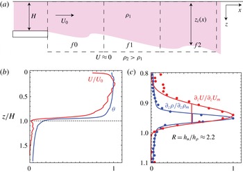
A schematic diagram of a vertical cross-section of the flow in figure 1 shows the main features of the experiment, including the nozzle exit geometry, the fluid densities, the acquisition frame positions, the mean flow velocities, the definition of the downstream dependent interface position $z_{i}(x)$ , and the coordinate axis of $\{x,z\}$ , where the top plate defines the origin $z=0$ . The Reynolds number of the gravity current, $Re=U_{0}H/\unicode[STIX]{x1D708}$ , lies in the range $2500<Re<3500$ , whereas the shear Reynolds number is $Re_{s}=U_{0}h_{u}/\unicode[STIX]{x1D708}$ with values in the range 700–1000. We expect the current to be fully turbulent (for more details on the turbulent aspects of the flow, see Odier et al. (Reference Odier, Chen and Ecke2014)) because of the pre-stirring of the injected fluid whereas the fluid in the tank is initially at rest. We use the first 1.1 cm region of $f0$ to define the initial conditions of the flow: the bulk Richardson number $Ri_{b}=g(\unicode[STIX]{x0394}\unicode[STIX]{x1D70C}/\unicode[STIX]{x1D70C}_{0})H/U_{0}^{2}$ based on the initial current height $H$ , $0.2<Ri_{b}<0.9$ ; the turbulent dissipation inside the current $0.9<\unicode[STIX]{x1D700}_{I}<1.3~\text{cm}^{2}~\text{s}^{-3}$ ; the ratio of $\unicode[STIX]{x1D700}$ inside the current and in the quiescent fluid $6<\unicode[STIX]{x1D700}_{I}/\unicode[STIX]{x1D700}_{O}<11$ ; the turbulent kinetic energy $0.9<K<2.3~\text{cm}^{2}~\text{s}^{-2}$ ; and the turbulent Reynolds number of the current $Re_{\ell }=u_{rms}^{\prime }\ell /\unicode[STIX]{x1D708}$ , where $\ell =K^{3/2}/\unicode[STIX]{x1D700}$ , $70<Re_{\ell }<270$ with estimated $R_{\unicode[STIX]{x1D706}}$ in the range 40–80. The higher values for quantities depending on velocity are for the ‘HV’ conditions whereas the lower ones are for ‘LV’ cases. In all cases, however, the current is more turbulent than the quiescent fluid, with an initial ratio of turbulent dissipation $\unicode[STIX]{x1D700}_{I}/\unicode[STIX]{x1D700}_{O}\sim 10$ , considerably less than the value of order $10^{3}$ in oceanic conditions (Price et al. Reference Price, Baringer, Lueck and Johnson1993) but large compared to typical laminar flow experiments where $\unicode[STIX]{x1D700}_{I}/\unicode[STIX]{x1D700}_{O}\sim 1$ and overall $\unicode[STIX]{x1D700}$ is small (i.e. laminar). The typical mean velocity and density profiles shown in figure 1(b) demonstrate that the velocity profile near the bottom of the exit nozzle ( $z/H=1$ ) is less steep than the density profile, reflecting that the velocity feels the no-slip boundary conditions of the channel before exiting whereas the density is uniform in the channel. In figure 1(c), we show the normalized velocity and density gradients which quantify the broader nature of the velocity gradient relative to the density gradient: the half-widths yield a ratio $R=h_{u}/h_{\unicode[STIX]{x1D70C}}\approx 2.2$ . These widths increase downstream as we shall see below.

Figure 1.

(a) Schematic of a vertical plane of the fluid flow with indications of densities, velocities, spatial coordinates, locations of imaging frames $f0-f2$ , and definition of interface position $z_{i}(x)$ . (b) Initial mean velocity $\langle U(z)\rangle /U_{0}$ and $\langle \unicode[STIX]{x1D703}(z)\rangle$ versus $z/H$ for LDHV conditions. (c) Corresponding initial normalized vertical gradients: $\langle \unicode[STIX]{x2202}_{z}U\rangle /\unicode[STIX]{x2202}_{z}U_{max}$ and $\langle \unicode[STIX]{x2202}_{z}\unicode[STIX]{x1D703}(z)\rangle /\unicode[STIX]{x2202}_{z}\unicode[STIX]{x1D703}_{max}$ .

Our choice of the experimental configuration presented above, namely a ‘wall jet’, as a representation of a gravity current has advantages and disadvantages. The advantages are the ability to create a turbulent input flow without relying on incompletely developing boundary layer instability inside the current to establish a turbulent interior (Odier et al. Reference Odier, Chen and Ecke2014), a more compact apparatus, and the ability to provide a lateral pressure gradient that does not need a slope to drive the flow; flow along a flat surface that transitions to flow along an incline is driven by the pressure gradient resulting from the accelerating flow in the inclined section. Regarding the latter, we believe that the physics of the problem should not depend sensitively on the source of the pressure gradient although one of the disadvantages of our set-up is that there is a transitional downstream length over which the mean flow negotiates the relative forces of bottom drag, interface drag and buoyancy. Thus, we use downstream frames $f1$ and $f2$ for stability analysis. The biggest observed effect on the flow is for the HDLV conditions where the current narrows as it exits the nozzle, shrinking from its initial 5 cm height in $f0$ to approximately 4 cm downstream in $f1$ and $f2$ . The instabilities described here do not appear to depend on this readjustment or other minor transitional variations.

3 Control parameters and instability properties

A stably stratified shear flow in a gravity current geometry is described by the current velocity $U_{0}$ , the density difference $\unicode[STIX]{x0394}\unicode[STIX]{x1D70C}$ and a characteristic length $h$ – sometimes the current height $H$ or in other cases the width of the vertical velocity shear layer $h_{u}$ . One has bulk control parameters of $Ri_{0}$ and $Re=U_{0}h/\unicode[STIX]{x1D708}$ for a fluid with viscosity $\unicode[STIX]{x1D708}$ . Typically, one ensemble-averages the density and downstream velocity fields in a fixed laboratory frame to obtain the global averages that define $h$ and thereby $Re$ and $Ri_{0}$ . Owing to vertical meandering of the interface and the intermittency of the flow, however, this averaging approach mixes different situations, e.g. unperturbed regions of the interface with no overturning and vertical wave displacement and regions of the interface with significant overturning. Here, as in natural environments, there are no idealized conditions or imposed experimental symmetries. Especially for relatively stable situations with higher $Ri$ , this ensemble averaging approach hides highly relevant features of stability and intermittency. For example, the entire range of $Ri_{0}$ for our data, based on an ensemble-averaged shear layer height, lies in the range 0.2–0.9, which would imply stability over most of the range according to the Miles–Howard (MH) criterion of 1/4. For this reason, we use a different approach to define average quantities and stability parameters. First, we separate unperturbed and perturbed sections of the interface by considering the vertical density profile at each position $x$ . If the density varies monotonically (aside from measurement fluctuations), this location is considered part of an ‘unperturbed’ interface. If there are significant changes in the sign of its slope, there is overturning and the interface is denoted as ‘perturbed’. Once this separation is completed, the vertical location $z_{i}$ of the unperturbed interface is defined as the location of maximum $\unicode[STIX]{x2202}\unicode[STIX]{x1D70C}/\unicode[STIX]{x2202}z$ , and the position relative to the interface is defined as $\tilde{z}=z-z_{i}$ . We then average density and velocity gradients in the unperturbed sections after centring them about the position of the unperturbed interface. We use the average gradients measured on the unperturbed sections of the interface at $\tilde{z}=0$ to define $Ri_{g_{0}}$ . This definition is the ‘global’ $Ri_{g}$ choice for numerical simulations (Hazel Reference Hazel1972; Alexakis Reference Alexakis2005) where the initial conditions are well defined by smooth functions. Our motivation here is the idea that conditions of stability in the unperturbed portions control the overturning and mixing that creates perturbed sections at later times. Regardless of the precise definition of $Ri$ , its overall range is approximately a factor of four between lowest and highest due to the doubling of density difference and/or downstream mean velocity in the current.

Figure 2.

Typical flow instability for four different flow conditions for downstream position $f2$ ( $x/H\geqslant 3$ ): (a)  $Ri_{g_{0}}=0.18$ (HVLD); (b)  $Ri_{g_{0}}=0.26$ (HVHD); (c)  $Ri_{g_{0}}=0.58$ (LVLD); and (d)  $Ri_{g_{0}}=0.68$ (LVHD). Image size is $7.2~\text{cm}\times 7.2~\text{cm}$ . Colour scale represents normalized density difference $\unicode[STIX]{x1D703}$ , red ( $\unicode[STIX]{x1D703}=1$ ) being the injected current and blue ( $\unicode[STIX]{x1D703}=0$ ) the ambient fluid. The lateral arrow in (a) denotes the horizontal downstream velocity $U_{0}$ . The left parts of (b–d) represent typical weakly perturbed interface conditions with HWI signature, whereas the right parts show KHI-like events. The vertical dashed arrows indicate the approximate vertical extent of the KHI events which are typical for the conditions shown.

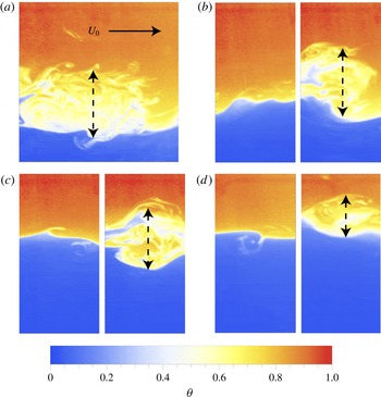
In figure 2, we show four example images of density fields that are characteristic of flows with varying degrees of stability for mean $Ri_{g_{0}}$ values of 0.18, 0.26, 0.58 and 0.68, corresponding to figure 2(a–d), respectively. Note that in all cases of KHI, the flow is inherently 3D because the turbulent conditions in the current provide fully 3D fluctuations that destroy the 2D symmetry seen in 2D simulations or at early time in 3D numerical simulations (Caulfield & Peltier Reference Caulfield and Peltier2000). When $Ri_{g}$ is small, similar to conditions used previously (Odier et al. Reference Odier, Chen, Rivera and Ecke2009, Reference Odier, Chen and Ecke2014), the flow is predominantly KHI-unstable with high resultant turbulent production along the interface between the moving and quiescent fluid, e.g. figure 2(a). At the other extreme of our range, when $Ri_{g}$ is larger, the flow is strongly stratified, and the available kinetic energy is often insufficient to induce vigorous vertical mixing, leading to intermittent KHI intermixed with wave-like modes of HWI type: figure 2(b–d) shows examples of HWI in the corresponding left image and KHI in the right image. In the most unstable case (a), the KHI-unstable events (chosen to be ‘typical’) are larger both vertically and horizontally than for higher $Ri$ cases (figure 2 b–d). The decreasing height of the disturbances with increasing $Ri$ reflects the changing competition between kinetic energy generated by shear and potential energy supplied by density differences. We revisit this feature below in describing the Thorpe length. The images in figure 2 are representative of states observed in both frames $f1$ and $f2$ . There are, however, quantitative differences between data from $f1$ and $f2$ , so that we sometimes plot data for each separately.

Figure 3.

(a) Density and velocity gradient profiles for HDLV case conditioned to the interface position $z_{i}$ , time/ensemble-averaged, and normalized by their maximum value. The vertical segments (thick for density, thin for velocity) show the half-widths and 20 % widths. (b) The corresponding HDLV $Ri_{g}$ profile computed from conditioned gradient profiles; peak ( $Ri_{g0}$ ) and trough ( $Ri_{g_{-}}$ and $Ri_{g_{+}}$ ) values are indicated. (c,d) The $Ri_{g}$ profiles for the other conditions as indicated in the plot. In all plots the vertical axis is the vertical distance to the interface $\tilde{z}=z-z_{i}$ normalized by the injection nozzle height $H$ and the data are from $f2$ ( $x/H>3$ ).

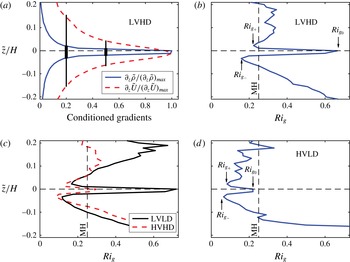
To better understand the nature of the instabilities that arise at different $Ri$ , we consider in figure 3(a) the detailed shape of the density and vertical velocity, averaged about the unperturbed interface. The gradients are normalized by their maximum value to facilitate comparison. The velocity gradient is broader than the density gradients as expected for a high- $Sc$ fluid (Carpenter et al. Reference Carpenter, Tedford, Rahmani and Lawrence2010) (quantitative details depend upon turbulent rather than molecular diffusion) and consistent with initial conditions of our flow. The difference between the density layer thickness $h_{\unicode[STIX]{x1D70C}}$ and the shear layer thickness $h_{u}$ affects the nature of the instability in linear stability analysis (Hazel Reference Hazel1972; Drazin & Reid Reference Drazin and Reid1981; Baines & Mitsudera Reference Baines and Mitsudera1994; Alexakis Reference Alexakis2005) where an important parameter is the thickness ratio $R=h_{u}/h_{\unicode[STIX]{x1D70C}}$ . For our different cases, we have $R\approx 3.3$ evaluated at half-maximum or $R\approx 6$ for 20 % maximum. The value of $R$ is sufficiently large to allow growth of HWI (Alexakis Reference Alexakis2005; Carpenter et al. Reference Carpenter, Tedford, Rahmani and Lawrence2010) and seems to be approximately independent of $Ri$ , indicative that the unperturbed interface is very similar among the cases considered. Evaluating the shear and density length scales from the gradient curves at 20 % maximum yields $h_{u}\approx 1.5$  cm and $h_{\unicode[STIX]{x1D70C}}\approx 0.25$  cm. Using this value of $h_{u}$ yields a range $0.07<Ri_{0}<0.31$ , in line with linear stability considerations. Inspection of the directly computed $Ri_{g}$ is even more revealing. The vertical profiles $Ri_{g}(z)$ displayed in figure 3(b–d) have local maxima at the interface, which we have defined as $Ri_{g_{0}}$ , and two minima $Ri_{g_{-}}$ and $Ri_{g_{+}}$ on either side of the maximum (positive $z$ is inside the current). The shape of $Ri_{g}(z)$ is consistent with theoretical expectations for cases where the density interface thickness is narrower than the shear-layer width of downstream velocity (Hazel Reference Hazel1972; Drazin & Reid Reference Drazin and Reid1981; Baines & Mitsudera Reference Baines and Mitsudera1994; Alexakis Reference Alexakis2005). Guided by the MH linear stability criterion, we define a second $Ri_{g}$ based on the minimum value near the unperturbed interface: $Ri_{g_{m}}=\text{Min}\{Ri_{g_{-}},Ri_{g_{+}}\}$ . For the data from $f2$ , $Ri_{g_{-}}<Ri_{g_{+}}$ except for smallest $Ri$ ; in $f1$ , they are closer to equal. How these minima evolve with the flow is an interesting question but beyond the scope of our present work. This characterization of $Ri_{g}(z)$ seems to be novel in the experimental description of an evolving stratified shear layer and represents a nuanced approach to understanding the stability of such flows.

4 Turbulent interface intermittency

We now have an approach for determining the stability parameter of the flow for different flow conditions. How then does the flow divide itself up between unperturbed and perturbed sections where we assume that the stability of the unperturbed sections controls the generation of unstable overturning sections? This approach is similar in spirit to understanding the transition between KHI and HWI, where KHI growth and collapse and coexisting KHI and HWI are observed in exchange-flow experiments (Hogg & Ivey Reference Hogg and Ivey2003) and in numerical simulations (Smyth & Peltier Reference Smyth and Peltier1989), and the spatiotemporal intermittency in tilted exchange flow situations (Tanino, Moisy & Hulin Reference Tanino, Moisy and Hulin2012). Significant spatial and temporal intermittency is also found in direct oceanic observations (Smyth, Moum & Caldwell Reference Smyth, Moum and Caldwell2001; Ivey et al. Reference Ivey, Winters and Koseff2008). With this approach in mind, we quantify the separation between perturbed and unperturbed interface in an intermittency fraction $F_{i}$ that is defined as the fraction of downstream locations $x$ with perturbed interface. 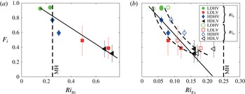The fraction $F_{i}$ is plotted in figure 4 as a function of $Ri_{g_{0}}$ and of $Ri_{g_{\pm }}$ as defined in figure 3(b,d). For each condition, we plot data from $f1$ and $f2$ separately; data from $f2$ have slightly higher $Ri$ than those from $f1$ in general. With increasing $Ri_{g}$ , $F_{i}$ decreases from of order one (all perturbed interface) for small $Ri_{g}$ towards zero (all stable interface) at larger $Ri_{g}$ . The rate of decrease, however, depends upon the definition of $Ri_{g}$ . The range of interface values $Ri_{g_{0}}$ is between 0.15 and 0.8, with an extrapolated zero intercept $F_{i}\rightarrow 0$ at $Ri_{g_{0}}\approx 1$ . The range of $Ri_{g_{m}}$ is between 0.05 and 0.2, and the intercept of $Fi$ is nicely suggestive of the MH criterion $Ri_{g}=1/4$ as shown by a linear fit (solid line) to the data in figure 4(b). We next discuss the reason for the decrease in $F_{i}$ and more details on the rate of that decrease.

Figure 4.

Intermittent fraction $F_{i}$ versus (a) $Ri_{g_{0}}$ and (b) $Ri_{g_{+}}$ and $Ri_{g_{-}}$ . Two values for each symbol represent different downstream frames $f1$ and $f2$ . Dashed curves are guides to the eye; vertical dashed line indicates the MH stability criterion $Ri_{g}=1/4$ . Solid lines are linear fits to the data (in (b) the fit is with respect to $Ri_{g_{m}}$ ).

Our interpretation of the observed intermittency scenario is that $F_{i}$ largely represents the fraction of KHI that would be expected to begin decreasing from unity for $Ri_{g}\approx 0.05{-}0.07$ (Smyth & Peltier Reference Smyth and Peltier1989; Hogg & Ivey Reference Hogg and Ivey2003) and to approach 0 at $Ri_{g}\simeq 1/4$ , consistent with the MH criterion based on our definition of $Ri_{g_{m}}$ . Holmboe instability becomes more prevalent at larger $Ri_{g}$ but does not contribute as much to $F_{i}$ due to the spatially localized nature of the instability involving sharp cusps at wave extrema positions versus the more horizontally extended KHI billows; an estimate for the contribution to $F_{i}$ from nonlinear HWI events of approximately 10 %–20 % can be obtained from idealized simulations and experiments (Carpenter et al. Reference Carpenter, Tedford, Rahmani and Lawrence2010) by taking the ratio of cusp lateral extent to HWI wavelength. Because the contribution of KHI to $F_{i}$ should go to zero at $Ri_{g}=1/4$ , any $F_{i}$ for $Ri_{g}>1/4$ , as suggested by the dashed line in figure 4(b) where $F_{i}$ decreases more rapidly than the linear trend for small $Ri_{g_{m}}$ and less rapidly for $Ri_{g_{m}}\approx 0.2$ , should be attributable to nonlinear Holmboe wave breaking. Overall our quantitative description of the transition from KHI to HWI is consistent with expectations (Hazel Reference Hazel1972; Drazin & Reid Reference Drazin and Reid1981; Baines & Mitsudera Reference Baines and Mitsudera1994; Carpenter et al. Reference Carpenter, Tedford, Rahmani and Lawrence2010) based on linear theory and idealized experiments in which KHI happens in the region around the interface where $Ri_{g}<1/4$ everywhere whereas HWI is nucleated away (displaced vertically) from the now stable interface position where $Ri_{g_{0}}>1/4$ . Given the successful interpretation of $Ri_{g_{m}}$ , we use it exclusively in the rest of our analysis.

Figure 5.

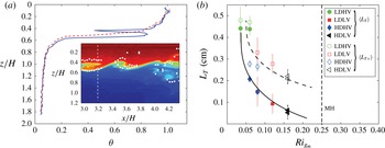
(a) Raw (solid, blue) and ordered (dashed, red) density profiles $z/H$ versus $\unicode[STIX]{x1D703}$ for the image shown in the inset. Vertical white dashed line in the inset indicates $x$ coordinate for the density profile. White solid circles show upper and lower boundaries of the overturning region. (b) Thorpe length for full interface $\langle L_{T}\rangle$ (solid symbols) and excluding zero values $\langle L_{T_{+}}\rangle$ (open symbols) versus $Ri_{g_{m}}$ . Vertical error bars are the standard deviations of the distributions. Dashed curve is $L_{T}=0.09Ri_{g}^{-1/2}$ and solid curve is $F_{i}L_{T}$ (where $F_{i}$ is the linear fit in figure 4 b); vertical dashed line indicates the MH stability criterion $Ri_{g}=1/4$ .

5 Thorpe length and overturning

We defined a stability criterion for unperturbed regions of the interface, and we discussed the evolution of the unperturbed/perturbed fraction $F_{i}$ with $Ri_{g}$ . We now naturally turn our attention towards the perturbed regions, trying in particular to study the distribution of their size, a crucial quantity in determining the amount of mixing that can be produced in these regions. To do so, we use the Thorpe length $L_{T}$ (Thorpe Reference Thorpe1977; Dillon Reference Dillon1982) as an identifier of overturning motion. As an example we consider in figure 5(a) the density profile for a single instantiation of the flow for HDLV conditions with perturbed interface. The solid line is the raw density profile corresponding to a vertical slice of the density field shown in the inset. The profile is reordered so that all elements are gravitationally stable, i.e. so that the density is a monotonic function of $z$ . The reordered profile is shown in figure 5(a) by the dashed (red) line. We eliminate spurious reordering due to noise (in regions of small density gradient, reordered $\unicode[STIX]{x1D6FF}z=\unicode[STIX]{x1D6FF}\unicode[STIX]{x1D70C}/\unicode[STIX]{x2202}_{z}\unicode[STIX]{x1D70C}$ can be anomalously large even for small $\unicode[STIX]{x1D6FF}\unicode[STIX]{x1D70C}$ resulting from measurement noise) by setting a threshold on the difference between the initial and reordered profile at four times the background density standard deviation.

The spatial displacements necessary to reorder the profile are called Thorpe displacements. These displacements are then used as weights to define the ‘disturbance region’: its centre is the weighted mean of the vertical position, and its vertical extent is the weighted quadratic mean of the distance from this centre. This disturbance region is marked by a pair of white dots in the inset of figure 5 for each downstream position $x$ of the perturbed interface. This systematic procedure accurately, and quite generally, identifies the disturbances as observed in the density contours. The Thorpe length is then defined as the standard deviation of the Thorpe displacements within the disturbance region; unperturbed interface has $L_{T}=0$ by definition. For the example in figure 5, the Thorpe length is 0.3 cm (compared to a disturbance region of approximately 1 cm).

We show in figure 5(b), as functions of $Ri_{g_{m}}$ , the mean Thorpe length $\langle L_{T}\rangle$ ensemble-averaged over all interface profiles for a particular flow condition and $\langle L_{T_{+}}\rangle$ , which is the average of only non-zero values of $L_{T}$ . The difference results from the intermittency fraction $F_{i}$ , where $\langle L_{T}\rangle =F_{i}\langle L_{T_{+}}\rangle$ ; $\langle L_{T}\rangle$ approaches zero, driven in part by the decreasing trend of $F_{i}$ whereas $\langle L_{T_{+}}\rangle$ decreases less rapidly. The decrease in $\langle L_{T_{+}}\rangle$ results from a competition between kinetic and potential energy so that lower $K$ and/or higher $\unicode[STIX]{x0394}\unicode[STIX]{x1D70C}$ decrease the vertical distance that an overturn can sustain, consistent with the qualitative trend observed in figure 2. The turbulent kinetic energy is defined as $K=1/2({u^{\prime }}^{2}+{v^{\prime }}^{2}+{w^{\prime }}^{2})\simeq 1/2({u^{\prime }}^{2}+2{w^{\prime }}^{2})$ (because of the vertical anisotropy in the system, one expects that $u^{\prime }>v^{\prime }>w^{\prime }$ because $u^{\prime }$ is enhanced by turbulent shear production and $w^{\prime }$ is suppressed by stabilizing buoyancy). The competition of kinetic and potential energy is related to the buoyancy length $L_{b}=w_{rms}/N\sim K^{1/2}/N$ , which is of the same order as $L_{T}$ in numerical simulations and microstructure measurements (Smyth et al. Reference Smyth, Moum and Caldwell2001). One can write this as $L_{T}\sim (w_{rms}/\unicode[STIX]{x2202}_{z}U)/(\unicode[STIX]{x2202}_{z}U/N)\sim (w_{rms}/\unicode[STIX]{x2202}_{z}U)Ri_{g}^{-1/2}\equiv \ell _{0}Ri_{g}^{-1/2}$ . If the KHI events that dominate the contribution to $L_{T}$ have similar $\ell _{0}=(w_{rms}/\unicode[STIX]{x2202}_{z}U)\approx \text{constant}$ , then $L_{T}=\ell _{0}Ri_{g}^{-1/2}$ with $\ell _{0}$ as an empirical constant (and correspondingly $F_{i}L_{T}$ for the fraction that includes zero values with the linear extrapolation for $F_{i}$ ), which fits the data fairly well with $\ell _{0}\approx 0.09$  cm (see figure 5 b). As a consistency check for the order of magnitude of the coefficient $\ell _{0}$ , we find that the ratio $\langle w_{rms}\rangle /\langle \unicode[STIX]{x2202}_{z}U\rangle \approx 0.25$  cm for the three highest $Ri_{g_{m}}$ values but 0.6 cm for $Ri_{g_{m}}\approx 0.05$ , perhaps suggesting that the basic relationship between $L_{T}$ and $Ri_{g}$ is no longer valid at small  $Ri_{g}$ .

Another test of the similarity of the overturning events as a function of $Ri_{g}$ is obtained by considering the full probability distribution of $L_{T}$ . To compare the probability distribution functions (p.d.f.s) for the different flow conditions, we first remove the fraction with $L_{T}=0$ and compute $P(L_{T_{+}})$ as shown in figure 6(a). We then normalize the p.d.f.s by subtracting the mean of the remaining values and dividing by the standard deviation of the distribution ( $\unicode[STIX]{x1D70E}_{L_{T+}}$ (cm): LDHV (0.24), LDLV (0.23), HDHV (0.17), and HDLV (0.14)). The resulting scaled p.d.f.s, shown in figure 6(c), collapse onto a self-similar curve with a strong exponential tail, $P(L_{T}^{\ast })\sim 10^{-L_{T}^{\ast }/L_{T_{0}}^{\ast }}$ , where $L_{T}^{\ast }=(L_{T_{+}}-\langle L_{T_{+}}\rangle )/\unicode[STIX]{x1D70E}_{L_{T+}}$ is the rescaled $L_{T_{+}}$ and $L_{T_{0}}^{\ast }=2$ . The collapse itself indicates that the physical process generating overturning events is the same for the different conditions once the mean $L_{T_{+}}$ and the size of the spread in $L_{T_{+}}$ (proportional to its standard deviation) are accounted for. So it seems that KHI events continue to dominate the contribution to the p.d.f. of $L_{T_{+}}$ despite a decreasing frequency proportional to $F_{i}$ with an overall average that decreases with increasing  $Ri_{g}$ .

Figure 6.

Probability distribution functions: (a) non-zero Thorpe length $P(L_{T_{+}})$ ; (b) kinetic energy $P(K)$ , where the arrows indicate the values of $K_{c}$ ; (c) normalized Thorpe length $L_{T}^{\ast }=(L_{T_{+}}-\langle L_{T_{+}}\rangle )/\unicode[STIX]{x1D70E}_{L_{T+}}$ and exponential fit to the positive values of $L_{T}^{\ast }$ (solid line) with $L_{T_{0}}^{\ast }=2$ ; and (d) normalized turbulent kinetic energy $K^{\ast }=(K-K_{c})/\unicode[STIX]{x1D70E}_{K}$ and corresponding exponential fit (dashed line) with $K_{0}^{\ast }=5$ . The legend differentiating curves is the same for all panels (a)–(d).

Can we say anything more about the origin of the exponential tails of the Thorpe length distribution? Since our experimental tools also allow us to accurately measure the velocity field fluctuations $\boldsymbol{u}^{\prime }=\boldsymbol{u}-\langle \boldsymbol{u}\rangle$ , some insight can be gained by considering the probability distribution of turbulent kinetic energy $P(K)$ . To confine our measure of $K$ to the vicinity of the interface, we average over a band of width 1 cm centred about the unperturbed interface contour. The resulting $P(K)$ is shown in figure 6(b). The fraction $1-F_{i}$ is proportional to the probability that a fluctuation in $K$ is of insufficient magnitude to overcome the potential energy barrier imposed by stratification. This allows one to obtain a lower cutoff $K_{c}$ defined by the condition $\int _{0}^{K_{c}}P(K)\,\text{d}K=1-F_{i}$ . The resulting values of $K_{c}$ are indicated by arrows in figure 6(b). The distribution of turbulent kinetic energy fluctuations able to perturb the interface is $P(K>K_{c})$ , which we shift to zero and renormalize to give unit probability, while dividing $K-K_{c}$ by the standard deviation of the new distribution $\unicode[STIX]{x1D70E}_{K}$ . The resulting distributions $P(K^{\ast })$ for our four different flow conditions are shown in figure 6(d), where there is good collapse of the distributions onto an exponential distribution of the form $P(K^{\ast })\sim 10^{-K^{\ast }/K_{0}^{\ast }}$ with $K_{0}^{\ast }\sim 5$ . This collapse provides a hint of the origin of the exponential scaling of $L_{T}$ , namely that the exponentially distributed fluctuations in $K$ induce varying degrees of overturning and produce an exponential distribution of $L_{T}$ since $L_{T}$ is a measure of the competition between the destabilizing influence of turbulent kinetic energy and the stabilizing influence of stratification. Using our empirical argument that $L\sim K^{1/2}$ also accounts roughly for the relationship between $L_{T_{0}}^{\ast }$ and $K_{0}^{\ast }$ , i.e.  $K_{0}^{\ast }\approx (L_{T_{0}}^{\ast })^{2}$ . A more detailed analysis of the competition between potential and kinetic energy seems possible using concepts of available potential energy (Winters et al. Reference Winters, Lombard, Riley and D’Asaro1995) but is beyond the scope of the present study.