


1 Introduction
When numerically solving hyperbolic conservation laws
 $$ \begin{align} u_t + f(u)_x =0 , \end{align} $$
Hamilton–Jacobi equations
 $$ \begin{align} \varphi_t + f(\varphi_x) =0 , \end{align} $$
or convection–diffusion equations
 $$ \begin{align} u_t + f(u)_x = (a(u) u_x)_x \end{align} $$
where
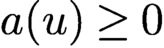 $a(u) \ge 0$
is small and possibly degenerate (i.e.
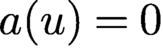 $a(u)=0$
for some values of u), or their multi-dimensional counterparts, a major difficulty is the possible lack of regularity of the exact solution, namely, the exact solution may contain discontinuities or sharp gradient regions, or discontinuous derivatives, regardless of the smoothness of the initial or boundary conditions (Smoller Reference Smoller1983, LeVeque Reference LeVeque1990).
If we are satisfied with first-order accurate schemes, then the class of monotone schemes (Crandall and Majda Reference Crandall and Majda1980, Crandall and Lions Reference Crandall and Lions1984) has excellent properties. Monotone schemes for scalar conservation laws can be proved to be non-linearly stable, measured by an
 $L^1$
contraction property, and to satisfy entropy conditions, leading to convergence with error estimates for bounded variation entropy solutions in multi-dimensions. Likewise, for Hamilton–Jacobi equations, monotone schemes can be proved to be
 $L^{\infty }$
-stable and convergent towards viscosity solutions with error estimates. However, first-order schemes converge very slowly, so to achieve the desired error level, one would often need to use a very refined mesh, which might be very inefficient or even impossible for multi-dimensional problems. On the other hand, traditional high-order accurate finite difference, finite volume, finite element or spectral schemes typically have spurious oscillations near discontinuities (the Gibbs phenomenon), which may pollute to smooth regions and may even lead to non-linear instability, causing blowups of the schemes. In fact, by the famous Godunov theorem, a linear scheme, which is defined to be linear for solving the linear conservation law (1.1) with
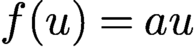 $f(u)=a u$
for a constant a, must be either oscillatory or only first-order accurate. Thus to obtain non-oscillatory schemes with higher than first-order accuracy, one must consider non-linear schemes, namely those schemes which are non-linear for (1.1) even with
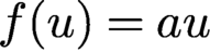 $f(u)=a u$
.
In computational fluid dynamics (CFD) and a few other areas of computational physics and engineering, the class of high-resolution schemes, mainly represented by the total variation diminishing (TVD) schemes (Harten Reference Harten1983, Osher and Chakravarthy Reference Osher and Chakravarthy1984), have been quite popular. The TVD schemes are non-linear schemes satisfying
 $$\begin{align*}\operatorname{\textit{TV}}(u^{n+1}) \le \operatorname{\textit{TV}}(u^n) , \end{align*}$$
where
 $u^n$
refers to the numerical solution at the time level
 $t^n$
, with the total variation semi-norm of a grid function defined by
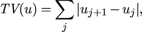 $$\begin{align*}\operatorname{\textit{TV}}(u) = \sum_j |u_{j+1} - u_j| , \end{align*}$$
where
 $u_j$
refers to the numerical solution at the spatial grid point
 $x_j$
. Usually, the TVD property is achieved through the application of various non-linear limiters such as the minmod limiter (Harten Reference Harten1983, LeVeque Reference LeVeque1990). TVD schemes can yield sharp and monotone discontinuity transitions and can achieve arbitrarily high-order accuracy in smooth and monotone regions (e.g. Osher and Chakravarthy Reference Osher, Chakravarthy and Dafermos1996); however, all TVD schemes have degeneracy of accuracy to first order near smooth extrema (Osher and Chakravarthy Reference Osher and Chakravarthy1984). It is clear that, even if the accuracy degenerates to first order only at one grid point, the global
 $L^1$
-error can be at most second-order, hence TVD or general high-resolution schemes are often referred to as second-order schemes, even though they can achieve arbitrarily high-order accuracy in smooth monotone regions (e.g. the very high-order TVD schemes in Osher and Chakravarthy Reference Osher, Chakravarthy and Dafermos1996). There are attempts in the literature to overcome this accuracy degeneracy problem, for example the total variation bounded (TVB) schemes (Shu Reference Shu1987), by relaxing the minmod limiter, but the TVB schemes involve a TVB parameter M, which must be estimated or tuned in order to achieve satisfactory performance (Shu Reference Shu1987, Cockburn and Shu Reference Cockburn and Shu1989), which restricts their wide applications.
The essentially non-oscillatory (ENO) schemes, first designed in Harten, Engquist, Osher and Chakravarthy (Reference Harten, Engquist, Osher and Chakravarthy1987), were a fundamental advance in achieving both arbitrarily high-order accuracy in smooth regions and sharp and essentially non-oscillatory discontinuity transitions. The key idea of ENO schemes is an approximation procedure, which we will survey in Section 2. Properties of the ENO procedure will also be discussed in Section2. The ENO schemes in Harten et al. (Reference Harten, Engquist, Osher and Chakravarthy1987) are in the finite volume framework, to be surveyed in Section 4.1. Soon after, Shu and Osher (Reference Shu and Osher1988, Reference Shu and Osher1989) developed efficient implementation of ENO schemes in the finite difference framework, to be surveyed in Section 4.2, with the so-called TVD Runge–Kutta time discretizations, to be surveyed in Section 7. ENO schemes have been under continuous development and improvement since their introduction, and have been popular in applications. This is demonstrated by the citation data. According to Google Scholar, the original ENO paper of Harten et al. (Reference Harten, Engquist, Osher and Chakravarthy1987), which was republished in 1997 by the Journal of Computational Physics as a classic paper (Shu Reference Shu1997, Harten, Engquist, Osher and Chakravarthy Reference Harten, Engquist, Osher and Chakravarthy1997), has been cited
 $3\,614$
times. The two finite difference ENO papers, Shu and Osher (Reference Shu and Osher1988) and Shu and Osher (Reference Shu and Osher1989), have been cited
 $4\,598$
and
 $2\,695$
times, respectively.
The weighted ENO (WENO) schemes, first designed in Liu, Osher and Chan (Reference Liu, Osher and Chan1994) and improved and extended in Jiang and Shu (Reference Jiang and Shu1996), were improved version of ENO schemes, overcoming some of the shortcomings of ENO schemes while maintaining their main advantages. The key idea of WENO schemes is again an approximation procedure, which we will survey in Section 3. Properties and different variants of the WENO procedure will also be discussed in Section 3. Finite volume WENO schemes (initialized in Liu, Osher and Chan Reference Liu, Osher and Chan1994) and finite difference WENO schemes (initialized in Jiang and Shu Reference Jiang and Shu1996) will be surveyed in Sections 4.1 and 4.2 respectively. WENO schemes have attracted even more attention than ENO schemes, both in algorithm development and in applications. According to Google Scholar, the original WENO paper of Liu et al. (Reference Liu, Osher and Chan1994) has been cited
 $2\,875$
times. The WENO paper of Jiang and Shu (Reference Jiang and Shu1996), which contains the classical fifth-order WENO scheme most popular in applications, has been cited
 $4\,964$
times.
2 The ENO interpolation and reconstruction procedures
The essentially non-oscillatory (ENO) scheme (Harten et al. Reference Harten, Engquist, Osher and Chakravarthy1987) is based on an ENO approximation procedure. In this section we will describe this procedure, emphasizing the details in the one-dimensional (1D) case and only sketching the procedure in the two-dimensional (2D) case.
2.1 The ENO interpolation procedure in 1D
Let us consider a piecewise smooth function
 $u(x)$
, either with compact support or with periodic boundary conditions, so that we do not need to consider the boundary. Assume that we have a mesh
 $$\begin{align*}\cdots < x_1 < x_2 < x_3 < \cdots \end{align*}$$
with
 $\Delta x_{i+{1}/{2}} = x_{i+1} - x_i$
, and
 $\Delta x = \max _i \Delta x_{i+{1}/{2}}$
. We assume that we are given the point value
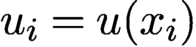 $u_i=u(x_i)$
of the function
 $u(x)$
, and we would like to obtain a high-order polynomial approximation
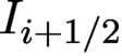
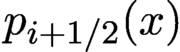 $p_{i+{1}/{2}}(x)$
, defined on
 $I_{i+{1}/{2}} = (x_i, x_{i+1})$
, which approximates the function
 $u(x)$
to high-order accuracy when
 $u(x)$
is smooth. This is a classical interpolation problem. For example, if we are given a four-point central stencil
 $$ \begin{align} S = \{ x_{i-1}, x_i, x_{i+1}, x_{i+2} \} {,} \end{align} $$
then there is a unique interpolation polynomial
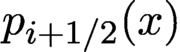 $p_{i+{1}/{2}}(x)$
, of degree at most three, that interpolates
 $u(x)$
in the stencil S:
 $$\begin{align*}p_{i+{1}/{2}}(x_j) = u_j, \quad j=i-1, i, i+1, i+2 . \end{align*}$$
We can write down this interpolation polynomial
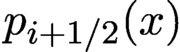 $p_{i+{1}/{2}}(x)$
in several different forms, for example in the Lagrange form or in the Newton form.
If the function
 $u(x)$
is smooth in the stencil S, then we have high-order accuracy, that is,
 $$ \begin{align} |u(x) - p_{i+{1}/{2}}(x)| \le C \Delta x^4, \quad x \in I_{i+{1}/{2}} . \end{align} $$
Here and below C would be used as a generic constant independent of the mesh parameters (here the mesh size
 $\Delta x$
), and it could take different values in each occurrence. We also have similar high-order accuracy for approximating the derivatives (with one order lower for each order of the derivative) and the integrals.
The problem, for piecewise smooth
 $u(x)$
, is accuracy near the discontinuity (or discontinuity of the derivative). If the stencil S contains a discontinuity of the function
 $u(x)$
, then the high-order accuracy (2.2) is no longer valid. Worse still, if the discontinuity is in S but not in
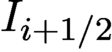 $I_{i+{1}/{2}}$
, the interpolation polynomial
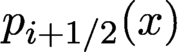 $p_{i+{1}/{2}}(x)$
is oscillatory in
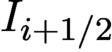 $I_{i+{1}/{2}}$
, in the sense that it has either an overshoot or an undershoot in
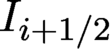 $I_{i+{1}/{2}}$
, with the overshoot/undershoot magnitude being a fixed percentage of the discontinuity size which does not decrease when the mesh size
 $\Delta x$
goes to zero (this is called the Gibbs phenomenon in the literature, especially in spectral methods). We remark that, miraculously, if the discontinuity is in the target cell
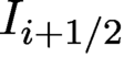 $I_{i+{1}/{2}}$
itself, the interpolation polynomial
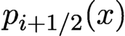 $p_{i+{1}/{2}}(x)$
is monotone in
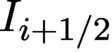 $I_{i+{1}/{2}}$
and does not show the Gibbs-type overshoot or undershoot there; see Harten, Osher, Engquist and Chakravarthy (Reference Harten, Osher, Engquist and Chakravarthy1986) for a proof of this (somewhat unexpected) fact.
The ENO idea in Harten et al. (Reference Harten, Engquist, Osher and Chakravarthy1987) is to choose the stencil S adaptively and automatically, based on the local smoothness of the function
 $u(x)$
. As we have seen from the discussion above, if the discontinuity is not in the target cell
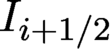 $I_{i+{1}/{2}}$
itself, we should avoid having the stencil S of interpolation containing this discontinuity. This is of course not possible if the choice for the pattern of the stencil is fixed for every cell
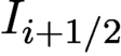 $I_{i+{1}/{2}}$
, for example the choice of the central stencil in (2.1). If we have the information of the exact location of the discontinuity, the choice of stencil is apparent. Given that the two end-points of the target cell
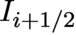 $I_{i+{1}/{2}}$
must be contained in the stencil, and if we must choose four points in the stencil to obtain a fourth-order cubic interpolation polynomial, then we could make the following choices.
-
• If there is no discontinuity inside the central stencil S defined in (2.1), or if the discontinuity is in the target cell
 $I_{i+{1}/{2}}$
itself, then we would use the central stencil S defined in (2.1).
-
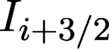
• Otherwise, if the discontinuity is in the cell
$I_{i+{3}/{2}}$
, then we should choose the left-biased stencil (2.3)
$$ \begin{align} S^{(-2)} = \{ x_{i-2}, x_{i-1}, x_{i}, x_{i+1} \}{.} \end{align} $$
-
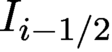
• Otherwise, if the discontinuity is in the cell
$I_{i-{1}/{2}}$
, then we should choose the right-biased stencil (2.4)
$$ \begin{align} S^{(0)} = \{ x_{i}, x_{i+1}, x_{i+2}, x_{i+3} \} . \end{align} $$
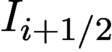


We remark that the strategy above assumes that discontinuities of the function
 $u(x)$
are isolated, so when the mesh size
 $\Delta x$
is small enough, we have at most one discontinuity in the stencil S determined by (2.1). The ENO and WENO procedures are both designed based on this assumption. However, they work well even when two discontinuities of the function collide, that is, when this assumption is violated, in extensive numerical experiments in the literature.
The problem with the strategy above is that we would need to know the existence and location of the discontinuity, based only on the point values
 $u_i$
of the function. This is difficult, especially when the mesh is coarse, namely when
 $\Delta x$
is not small enough. The novelty of the ENO procedure in Harten et al. (Reference Harten, Engquist, Osher and Chakravarthy1987) is that, based on extensive numerical experiments, the authors identified a strategy to automatically choose the stencil S which works well both in the asymptotic regime (when
 $\Delta x$
is small) and in the pre-asymptotic regime. The strategy to choose the local stencil
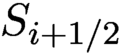 $S_{i+{1}/{2}}$
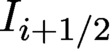
, associated with the cell
 $I_{i+{1}/{2}}$
to construct the interpolation polynomial
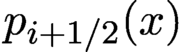 $p_{i+{1}/{2}}(x)$
, is as follows.
-
• Compute the Newton divided differences of
$u(x)$
. For
$j= \ldots 1,2,3, \ldots ,$
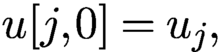
then for
$$\begin{align*}u[j,0] = u_j, \end{align*}$$
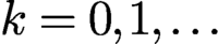
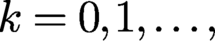
$k=0,1, \ldots $
and all j,
$$\begin{align*}u[j,k+1] = \displaystyle \frac{u[j+1,k]-u[j,k]}{x_{j+1+k}-x_j} . \end{align*}$$
-
• Choose the initial stencil
$S^{(0)}$
to only contain the two end-points of the target cell
$I_{i+{1}/{2}}$
: Then, each time, only one point is added to the stencil, the left point or the right point, depending on which one gives a ‘smoother’ stencil. For
$$\begin{align*}S^{(0)} = \{ x_i, x_{i+1} \} . \end{align*}$$
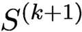
$k=0,1,\ldots ,$
suppose the leftmost point in the stencil
$S^{(k)}$
is
$x_{i_k}$
; then the next stencil
$S^{(k+1)}$
is determined as follows.
-
– If
$ | u[i_k-1,k] | < |u[i_k,k]|$
, then
$S^{(k+1)} = S^{(k)} \cup \{ x_{i_k-1} \}$
. -
– Otherwise,
$S^{(k+1)} = S^{(k)} \cup \{ x_{i_k+k+2} \}$
.
-










The final stencil is taken as
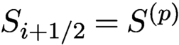 $S_{i+{1}/{2}}=S^{(p)}$
, where
 $p+1$
is the degree of the interpolation polynomial that we would like to use. Once the stencil
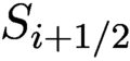 $S_{i+{1}/{2}}$
is determined, we can obtain the interpolation polynomial
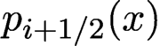 $p_{i+{1}/{2}}(x)$
either by the Newton form or by the Lagrangian form. If we are only interested in obtaining specific information about the interpolation polynomial
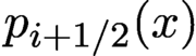 $p_{i+{1}/{2}}(x)$
, for example its value at the mid-point
 $x_{i+{1}/{2}} = \tfrac 12 (x_i + x_{i+1})$
or the derivative at the left point
 $x_i$
or the right point
 $x_{i+1}$
, we could also obtain such information directly from a linear combination of the point values
 $u_j$
in the stencil
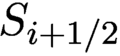 $S_{i+{1}/{2}}$
without explicitly constructing the polynomial
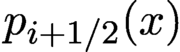 $p_{i+{1}/{2}}(x)$
. For explicit formulas and tables associated with this process, we refer to Shu (Reference Shu and Cockburn1998), for example.
We remark that, in the choice of the ENO stencil, we start with
 $S^{(0)}$
which consists of the two end-points of the target interval
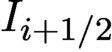 $I_{i+{1}/{2}}$
. This is actually needed for the conservation property when ENO is used to form a scheme for solving the hyperbolic conservation laws (1.1). If the ENO procedure is used for other purposes, the starting stencil could also contain just one point (e.g.
 $x_i$
) or more than two points, to suit the particular need of the applications.
The ENO procedure outlined above may end up with a very biased stencil, especially when the order of accuracy is high, for certain functions whose derivatives (and hence divided differences) are monotone. For example, for the function
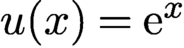 $u(x)=\mathrm {e}^x$
, every derivative is monotonically increasing, hence the divided differences as a function of the first point in the stencil are also monotonically increasing, resulting in an ENO stencil which is biased to the left. This may cause some stability and accuracy issues when used to solve time-dependent hyperbolic equations (Rogerson and Meiburg Reference Rogerson and Meiburg1990). To overcome this difficulty, a modified ENO procedure with the choice biased to a target final stencil was defined in Shu (Reference Shu1990). The only modification to the classical ENO procedure as outlined above is as follows. We have a preferred target final stencil
 $S^{c}$
, with the leftmost point
 $x_{i_c}$
, for example the central stencil S determined in (2.1) for which
 $x_{i_c}=x_{i-1}$
. Before the leftmost point of the current stencil
 $S^{(k)}$
reaches
 $x_{i_c}$
, we would use a factor to encourage the next stencil
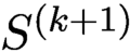 $S^{(k+1)}$
to shift to the left; when the leftmost point of the current stencil
 $S^{(k)}$
has already reached or passed
 $x_{i_c}$
, then we would use the factor to discourage this shift. To be more specific, we choose a biasing factor
 $b>1$
(
 $b=2$
is suggested in Shu Reference Shu1990). If the leftmost point in the stencil
 $S^{(k)}$
is
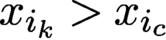 $x_{i_k}>x_{i_c}$
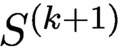
, then the next stencil
 $S^{(k+1)}$
is determined as follows.
-
• If
$ | u[i_k-1,k] | < b |u[i_k,k]|$
, then
$S^{(k+1)} = S^{(k)} \cup \{ x_{i_k-1} \}$
. -
• Otherwise,
$S^{(k+1)} = S^{(k)} \cup \{ x_{i_k+k+2} \}$
.



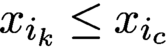
On the other hand, if the leftmost point in the stencil
 $S^{(k)}$
is
 $x_{i_k} \le x_{i_c}$
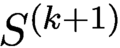
, then the next stencil
 $S^{(k+1)}$
is determined as follows.
-
• If
$ b | u[i_k-1,k] | < |u[i_k,k]|$
, then
$S^{(k+1)} = S^{(k)} \cup \{ x_{i_k-1} \}$
. -
• Otherwise,
$S^{(k+1)} = S^{(k)} \cup \{ x_{i_k+k+2} \}$
.



The final stencil from the modified ENO procedure has a better chance of being the target preferred stencil in the smooth regions of
 $u(x)$
.
2.2 The ENO reconstruction procedure in 1D
While the ENO interpolation procedure as described in Section 2.1 is the most basic one, a slightly different ENO reconstruction procedure is more relevant for the construction of conservative schemes for solving hyperbolic conservation laws (1.1). We will describe this reconstruction procedure and point out its relationship to the ENO interpolation procedure described in the previous section.
Let us use a slightly different notation which is more standard for finite volume schemes. We denote discretization of the line R into cells
 $I_i= (x_{i- {1}/{2}}, x_{i+ {1}/{2}})$
, where
 $\cdots x_{{1}/{2}} < x_{{3}/{2}} < x_{{5}/{2}} < \cdots $
,
 $\Delta x_i = x_{i+ {1}/{2}} - x_{i- {1}/{2}}$
is the mesh size of cell
 $I_i$
, and
 $\Delta x = \max _i \Delta x_i$
. We assume that we are given the cell averages of a piecewise smooth function
 $u(x)$
:
 $$\begin{align*}\bar{u}_i = \displaystyle \frac{1}{\Delta x_i} \int_{x_{i- {1}/{2}}}^{x_{i+ {1}/{2}}} u(x) \,\text{d} x, \quad i= \ldots 1,2,3, \ldots {,} \end{align*}$$
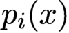
and we would like to obtain a high-order polynomial approximation
 $p_{i}(x)$
, defined on
 $I_{i}$
, which approximates the function
 $u(x)$
to high-order accuracy when
 $u(x)$
is smooth. Similar to an interpolation problem, the reconstruction problem is based on a stencil, for example a central stencil
 $S= \{ I_{i-1}, I_{i}, I_{i+1} \}$
, and we would like to find a quadratic polynomial
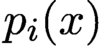 $p_{i}(x)$
such that
 $$\begin{align*}\displaystyle \frac{1}{\Delta x_j} \int_{x_{j- {1}/{2}}}^{x_{j+ {1}/{2}}} p_i(x) \,\text{d} x = \bar{u}_j, \quad j=i-1, i, i+1. \end{align*}$$
We could of course use ideas similar to interpolation to establish the existence and uniqueness of such reconstruction polynomials
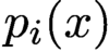 $p_i(x)$
and to obtain them explicitly. However, it is more convenient to use the so-called ‘reconstruction via primitive functions’ procedure to convert the reconstruction problem to the interpolation problem described in the previous section, and then we can simply use the ENO procedure spelled out there.
Define
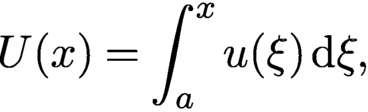 $$ \begin{align} U(x) = \int_a^x u(\xi) \,\text{d} \xi {,} \end{align} $$
where the lower limit a is not important and could be chosen as
 $a=x_{i_0-{1}/{2}}$
, where
 $I_{i_0}$
is the first cell of interest to us, for convenience. We then have
 $U(x_{i_0-{1}/{2}})=0$
and, for any
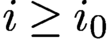 $i \ge i_0$
,
 $$\begin{align*}U(x_{i+{1}/{2}})= \int_{x_{i_0-{1}/{2}}}^{x_{i+{1}/{2}}} u(\xi) \,\text{d} \xi = \sum_{j=i_0}^i \int_{x_{j- {1}/{2}}}^{x_{j+ {1}/{2}}} u(\xi) \,\text{d} \xi = \sum_{j=i_0}^i \bar{u}_j \Delta x_j . \end{align*}$$
That is, if we know the cell averages
 $\bar {u}_j$
of
 $u(x)$
, we also know the point values
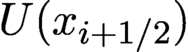 $U(x_{i+{1}/{2}})$
of the primitive function
 $U(x)$
as defined in (2.5). We can then invoke the interpolation procedure described in Section 2.1 for
 $U(x)$
. For example, if we use a central stencil
 $\tilde {S} = \{ x_{i-{3}/{2}}, x_{i-{1}/{2}}, x_{i+{1}/{2}}, x_{i+{3}/{2}} \}$
, obtaining a cubic interpolation polynomial
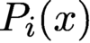 $P_i(x)$
satisfying
 $$\begin{align*}P_i(x_{j+{1}/{2}}) = U(x_{j+{1}/{2}}), \quad j=i-2, i-1, i, i+1 {,} \end{align*}$$
then
 $p_i(x) = \tfrac {\mathrm {d}}{\mathrm {d} x} P_i(x)$
would be the corresponding quadratic reconstruction polynomial for
 $u(x)$
on the central stencil
 $S = \{ I_{i-1}, I_{i}, I_{i+1} \}$
, since
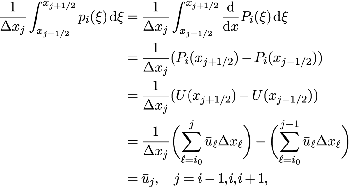 $$ \begin{align*} \begin{aligned} \displaystyle \frac{1}{\Delta x_j} \int_{x_{j- {1}/{2}}}^{x_{j+ {1}/{2}}} p_i(\xi) \,\text{d} \xi &= \displaystyle \frac{1}{\Delta x_j} \int_{x_{j- {1}/{2}}}^{x_{j+ {1}/{2}}} \displaystyle \frac {\mathrm{d}}{\mathrm{d} x} P_i(\xi) \,\text{d} \xi \\ &= \displaystyle \frac{1}{\Delta x_j} ( P_i(x_{j+ {1}/{2}}) - P_i(x_{j- {1}/{2}}) ) \\ &= \displaystyle \frac{1}{\Delta x_j} ( U(x_{j+ {1}/{2}}) - U(x_{j- {1}/{2}}) ) \\ &= \displaystyle \frac{1}{\Delta x_j} \biggl( \sum_{\ell=i_0}^j \bar{u}_{\ell} \Delta x_{\ell} \biggr) - \biggl( \sum_{\ell=i_0}^{j-1} \bar{u}_{\ell} \Delta x_{\ell} \biggr) \\ &= \bar{u}_{j}, \quad j=i-1,i,i+1 {,} \end{aligned} \end{align*} $$
where in the third equality we used the fact that
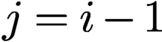 $j=i-1$
, i or
 $i+1$
, hence both
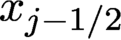 $x_{j- {1}/{2}}$
and
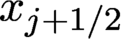 $x_{j+ {1}/{2}}$
are in the interpolation stencil
 $\tilde {S}$
for the interpolation polynomial
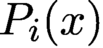 $P_i(x)$
.
Because of this relationship between reconstruction and interpolation, we do not need to consider a separate ENO reconstruction procedure: we can simply use the ENO interpolation procedure described in the previous section for obtaining
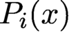 $P_i(x)$
, then take its derivative to obtain the reconstruction polynomial
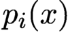 $p_i(x)$
. We also note that the first-order divided difference of
 $U(x)$
is
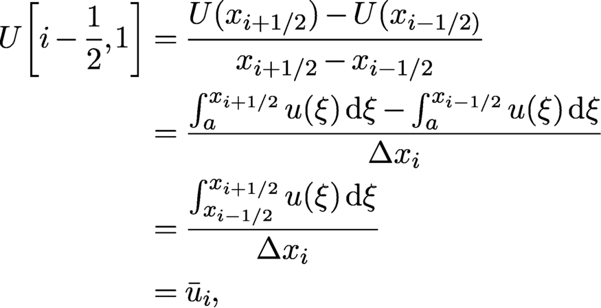 $$ \begin{align*} U \biggl[ i-\displaystyle \frac 12,1 \biggr] & = \displaystyle \frac{U(x_{i+ {1}/{2}})-U(x_{i- {1}/{2})}}{x_{i+ {1}/{2}} - x_{i- {1}/{2}}}\\ &=\displaystyle \frac{ \int_{a}^{x_{i+ {1}/{2}}} u(\xi) \,\text{d} \xi - \int_{a}^{x_{i- {1}/{2}}} u(\xi) \,\text{d} \xi}{\Delta x_i}\\ &= \displaystyle \frac{ \int_{x_{i- {1}/{2}}}^{x_{i+ {1}/{2}}} u(\xi) \,\text{d} \xi}{\Delta x_i}\\ &=\bar{u}_i , \end{align*} $$
and hence the first- and higher-order divided differences of
 $U(x)$
can be written as the divided differences of
 $\bar {u}$
, that is, there is no need to explicitly compute the divided differences of
 $U(x)$
at all (since the zeroth-order divided difference of
 $U(x)$
is not needed when computing
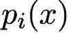 $p_i(x)$
, which is the derivative of the interpolating polynomial
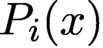 $P_i(x)$
).
We again refer to Shu (Reference Shu and Cockburn1998) for explicit formulas and tables associated with the ENO reconstruction process.
2.3 Properties of ENO interpolation and reconstruction procedures
Besides the standard approximation properties of the ENO interpolation and reconstruction polynomials when the function is smooth in the stencil, we also have several properties of the ENO procedure for piecewise smooth functions in relation to its (essentially) non-oscillatory performance.
2.3.1 Total variation bounded property for piecewise smooth functions
Harten et al. (Reference Harten, Osher, Engquist and Chakravarthy1986) proved the following total variation bounded (TVB) property of the ENO interpolation and ENO reconstruction procedures, as described in Sections 2.1 and 2.2.
For a piecewise smooth function
 $u(x)$
with isolated discontinuities, both the ENO interpolation polynomial
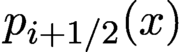 $p_{i+ {1}/{2}}(x)$
, as described in Section 2.1, and the ENO reconstruction polynomial
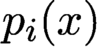 $p_i(x)$
, as described in Section 2.2, have the following TVB property: there exists a function
 $q(x)$
satisfying
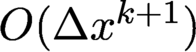
 $$\begin{align*}q(x) = p_r(x) + O(\Delta x^{k+1}), \quad x \in I_r \end{align*}$$
(where
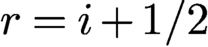 $r=i+ 1/2$
for the ENO interpolation and
 $r=i$
for the ENO reconstruction), such that
 $$\begin{align*}\operatorname{\textit{TV}} (q) \leq \operatorname{\textit{TV}}(u) + O(\Delta x^{k}). \end{align*}$$
Here,
 $\operatorname {\mathit {TV}}$
denotes the bounded variation semi-norm of the function. This property completely rules out the possibility of Gibbs oscillations near discontinuities, and is responsible for the (essentially) non-oscillatory performance of ENO approximations.
A crucial fact used in the proof of the TVB property above is that if the discontinuity is inside the target cell
 $I_r$
, then the interpolation or reconstruction polynomial
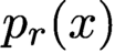 $p_r(x)$
is monotone in
 $I_r$
. The proof of this fact is also provided in Harten et al. (Reference Harten, Osher, Engquist and Chakravarthy1986). Away from the discontinuities, the ENO interpolation or reconstruction polynomial has a stencil which does not contain any discontinuity, hence the classical approximation result applies, giving an error estimate at the truncation error
 $O(\Delta x^{k+1})$
.
2.3.2 The sign property
The TVB property described in the previous subsection is an approximation result for piecewise smooth functions. That is, it holds only if the point values (for the ENO interpolation) or cell averages (for the ENO reconstruction) are exact from the piecewise smooth function
 $u(x)$
. If the ENO procedure is used to solve a time-dependent partial differential equation (PDE), such as the conservation law equation (1.1), at later time the point values or cell averages of the numerical solution are already polluted by accumulated numerical errors, hence the TVB property can no longer be rigorously proved.
It would be desirable to get a stability result for the ENO procedure which does not depend on the smoothness of the function
 $u(x)$
. The following ‘sign property’, which was proved in Fjordholm, Mishra and Tadmor (Reference Fjordholm, Mishra and Tadmor2013b), establishes such a stability result.
Sign property for the ENO reconstruction. For an ENO reconstruction procedure described in Section 2.2, the jump at the cell interface from the ENO reconstruction in two adjacent cells, namely
 $u^+_{j+{1}/{2}} = p_{j+1} (x_{j+{1}/{2}})$
and
 $u^-_{j+{1}/{2}} = p_{j} (x_{j+{1}/{2}})$
, has the same sign as the jump in the given cell averages:
 $$\begin{align*}(\bar{u}_{i+1}-\bar{u}_i)(u^+_{j+{1}/{2}}-u^-_{j+{1}/{2}}) \ge 0 \quad \text{for all}\ i. \end{align*}$$
Moreover, their ratio is uniformly bounded:
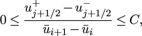 $$\begin{align*}0 \le \displaystyle \frac{u^+_{j+{1}/{2}}-u^-_{j+{1}/{2}}}{\bar{u}_{i+1}-\bar{u}_i} \le C {,} \end{align*}$$
where C is a universal constant depending only on the polynomial degree k used in the ENO interpolation.
A similar result is also valid for the ENO interpolation procedure in terms of its jumps of the derivatives, as described in Section 2.1.
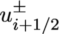
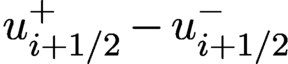
The sign property is somewhat surprising. The ENO reconstruction values
 $u^{\pm }_{i+{1}/{2}}$
are obtained from several neighbouring cell averages in the ENO reconstruction, but the sign of the jump
 $u^+_{i+{1}/{2}}-u^-_{i+{1}/{2}}$
is solely determined by the immediate neighbouring cell averages
 $\bar {u}_i$
and
 $\bar {u}_{i+1}$
; the other cell averages further away but still in the ENO reconstruction stencil seem to play no role in the sign property. This is a very strong stability result. It excludes the saw-tooth or zigzag pattern in the reconstruction (e.g. the given cell averages are increasing from cell i to cell
 $i+1$
, but the reconstructed values at the cell interface
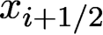 $x_{i+{1}/{2}}$
is decreasing). It also guarantees that the jump at any interface can be at most a fixed factor larger than the difference of the neighbouring cell averages.
Note that the sign property cannot be proved for the biased ENO procedure described in Section 2.1. Moreover, it can only be proved for a very special class of the WENO procedure (Fjordholm and Ray Reference Fjordholm and Ray2016).
This sign property could be used to obtain arbitrarily high-order accurate entropy stable ENO schemes for systems of conservation laws (Fjordholm, Mishra and Tadmor Reference Fjordholm, Mishra and Tadmor2013a).
2.4 The ENO procedure based on non-polynomial functions
Similar ENO interpolation and reconstruction procedures can of course also be designed for non-polynomial approximation functions. In Christofi (Reference Christofi1996), such an ENO procedure was designed for trigonometric polynomial basis functions. A key ingredient in such a design is to define suitable divided differences, which could be linked to derivatives of the function
 $u(x)$
and hence be used to choose the ENO stencil appropriately. Such ENO procedures could be useful for certain classes of functions, for example high-frequency wave functions, for which trigonometric polynomials could be expected to provide better approximations than algebraic polynomials. Other types of basis functions (such as exponential-type functions to resolve better boundary or internal layers with sharp gradients) could of course also be used.
2.5 Multi-dimensions and unstructured meshes
For two and higher dimensions, there is a difference between tensor product-type meshes and unstructured meshes.
For tensor product-type meshes, if a finite difference ENO interpolation is desired, it is usually sufficient just to use one-dimensional interpolations, keeping all the other spatial variables fixed. This would be the case for the finite difference ENO scheme in multi-dimensions, for example, to be described in Section 4.2. If a finite volume ENO reconstruction is desired, it is usually a procedure to obtain point values of a function from the given multi-dimensional cell averages (we use two dimensions as examples):
 $$\begin{align*}\tilde{\bar{u}}_{i,j} = \displaystyle \frac {1}{\Delta x_i \Delta y_j} \int_{y_{j-{1}/{2}}}^{y_{j+{1}/{2}}} \int_{x_{i-{1}/{2}}}^{x_{i+{1}/{2}}} u(x,y) \,\text{d} x \,\text{d} y {,} \end{align*}$$
where
 $I_{i,j} = (x_{i-{1}/{2}},x_{i+{1}/{2}}) \times (y_{j-{1}/{2}}, y_{j+{1}/{2}})$
is a two-dimensional tensor product cell, with mesh sizes
 $\Delta x_i = x_{i+{1}/{2}} - x_{i-{1}/{2}}$
and
 $\Delta y_j = y_{j+{1}/{2}} - y_{j-{1}/{2}}$
. Here, we use bar to denote the cell averaging operator in x and tilde to denote the cell averaging operator in y. If we apply a one-dimensional ENO reconstruction procedure in x, with the y index j fixed, we would be able to ‘de-cell average’ in the x variable to obtain the ‘point values’ (relative to the x variable), which are in fact still a cell average in y. For example, we could get
 $$\begin{align*}\tilde{u}^-_{i+ {1}/{2}, j} = \displaystyle \frac {1}{\Delta y_j} \int_{y_{j-{1}/{2}}}^{y_{j+{1}/{2}}} (x_{i+{1}/{2}}^-, y) \,\text{d} y {.} \end{align*}$$
Then we could fix the x index
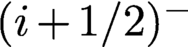 $(i+1/2)^-$
and apply another one-dimensional ENO reconstruction procedure in y, to ‘de-cell average’ in the y variable to obtain the point values of the function
 $u(x)$
at
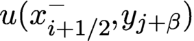 $u(x_{i+{1}/{2}}^-, y_{j+ \beta })$
, for example, where
 $y_{j+ \beta }$
could be a Gauss quadrature point along the cell boundary
 $(y_{j-{1}/{2}}, y_{j+{1}/{2}})$
. This would be the case for the finite volume ENO scheme in multi-dimensional tensor product meshes, for example, to be described in Section 4.1.3.
For unstructured meshes, for example triangular meshes in two dimensions, we cannot use one-dimensional ENO procedures directly. However, the basic ENO philosophy is still valid, namely we obtain interpolation or reconstruction based on several fixed stencils containing enough triangles to build polynomial approximations either by exact interpolation or reconstruction, or by a least-squares procedure, then we choose a final ‘smoothest’ stencil to obtain the ENO approximation polynomial. A key ingredient in such a design is still to define suitable ‘divided differences’, which could be linked to derivatives of the function
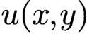 $u(x,y)$
and hence be used to choose the ENO stencil appropriately. Such an ENO scheme on unstructured meshes was first constructed in Abgrall (Reference Abgrall1994).
For more details about the two- (and higher-) dimensional ENO reconstruction procedures, we refer to the references listed above and to Shu (Reference Shu and Cockburn1998).
3 The WENO interpolation and reconstruction procedures
While the ENO interpolation and reconstruction procedures described in Section 2 are very popular in applications, they do have a few shortcomings. The first is that several candidate stencils have been considered in the ENO stencil choice process, but only one of them is finally adopted and the remaining ones have been abandoned. While this certainly makes sense near discontinuities as we do not want interpolation or reconstruction across discontinuities, in smooth regions (which form the majority part in the computational domain for piecewise smooth functions) it might be more beneficial to use information from all the candidate stencils, as none of them contains any discontinuity. Also, the ‘digital’ way of choosing the stencil and hence the ENO approximation makes the procedure less smooth: the interpolated or reconstructed value is at most Lipschitz-continuous with respect to the given data, but not smoother. This might cause problems in steady-state convergence. Finally, the ENO stencil choice process might choose ‘downwind-biased’ stencils systematically, hence affecting the stability and achieved order of accuracy, as showed by the numerical experiments in Rogerson and Meiburg (Reference Rogerson and Meiburg1990). Even though the biased ENO procedure (Shu Reference Shu1990) reviewed in Section 2.1 addresses this issue, it would be better to have a more systematic way of ensuring stable stencils for solving hyperbolic conservation laws.
The weighted ENO (WENO) procedure, which is an extension of the ENO procedure, could overcome the shortcomings mentioned above while maintaining the good properties of ENO approximations. The idea is to use a convex combination of interpolations or reconstructions from different candidate stencils, rather than using only one of them, as is the case for ENO. Of course, the crucial ingredient is then the choice of the combination coefficients, also called non-linear weights, which should be chosen to fulfil the following two properties. (1) When the solution is smooth in all candidate stencils, the non-linear weights should be chosen to be very close to the so-called ‘linear weights’, which could provide the highest possible order of accuracy from the combined stencil. (2) When a particular candidate stencil contains a discontinuity, while there is at least one other candidate stencil which does not contain any discontinuity, then the candidate stencil containing a discontinuity should be assigned a very small weight, hence its influence towards the approximation is negligible. This would avoid spurious oscillations in the same way as ENO.
The first WENO procedure was introduced by Liu et al. (Reference Liu, Osher and Chan1994), who developed a third-order WENO reconstruction procedure and used it to form a finite volume scheme for solving hyperbolic conservation laws. Their procedure can produce a
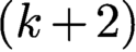 $(k+2)$
th-order WENO scheme from the same stencils as for a
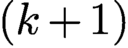 $(k+1)$
th-order ENO scheme. Jiang and Shu (Reference Jiang and Shu1996) established a general framework for forming a
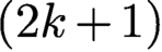 $(2k+1)$
th-order WENO approximation from a
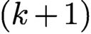 $(k+1)$
th-order ENO stencil, and constructed a finite difference WENO scheme based on the fifth-order WENO approximation procedure, which is more efficient for solving multi-dimensional conservation laws than finite volume schemes. The fifth-order WENO scheme constructed by Jiang and Shu (Reference Jiang and Shu1996) has been the most commonly used WENO scheme in applications. Subsequently, there have been numerous papers on extending, adapting and applying WENO schemes in the literature. In this section we will briefly describe the basic ideas and various versions of WENO approximation procedures.
3.1 The classical WENO procedures
The classical WENO approximation procedure, initialized in Liu et al. (Reference Liu, Osher and Chan1994) and generalized in Jiang and Shu (Reference Jiang and Shu1996), will be summarized in this subsection. A
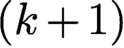 $(k+1)$
th-order ENO scheme can be ‘upgraded’ to a
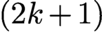 $(2k+1)$
th-order WENO approximation as follows. To make the presentation simple, we concentrate on the
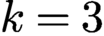 $k=3$
case, that is, the fifth-order WENO procedure of Jiang and Shu (Reference Jiang and Shu1996).
Let us look at the third-order ENO reconstruction procedure in Section 2.2. The third-order ENO approximation
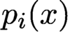 $p_i(x)$
in cell
 $I_i$
, which is a quadratic polynomial, could be one of the following three polynomials:
-
•
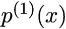
$p^{(1)}(x)$
, corresponding to the quadratic reconstruction polynomial over the left-biased stencil
$S^{(1)} = \{ I_{i-2}, I_{i-1}, I_{i} \}$
, -
• or
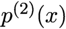
$p^{(2)}(x)$
, corresponding to the quadratic reconstruction polynomial over the central stencil
$S^{(2)} = \{ I_{i-1}, I_{i}, I_{i+1} \}$
, -
• or
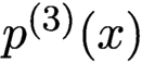
$p^{(3)}(x)$
, corresponding to the quadratic reconstruction polynomial over the right-biased stencil
$S^{(1)} = \{ I_{i}, I_{i+1}, I_{i+2} \}$
.



The idea of WENO is to form a convex combination of the three ENO candidate polynomials
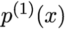 $p^{(1)}(x)$
,
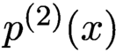 $p^{(2)}(x)$
and
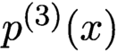 $p^{(3)}(x)$
. Typically, we are only interested in a particular value of the reconstruction, for example the approximation at the right boundary of cell
 $I_i$
, so we would like to form a convex combination
 $$ \begin{align} u^-_{i + {1}/{2}} = w_1 p^{(1)}(x_{i + {1}/{2}}) + w_2 p^{(2)}(x_{i + {1}/{2}}) + w_3 p^{(3)}(x_{i + {1}/{2}}) \end{align} $$
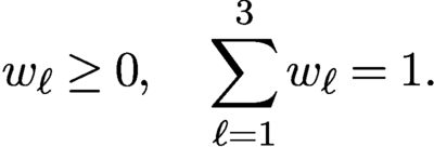
where the non-linear weights satisfy
 $$ \begin{align} w_{\ell} \ge 0, \quad \sum_{\ell=1}^3 w_{\ell} =1 . \end{align} $$
Clearly, for any such choices of the non-linear weights, we have at least third-order accuracy
 $$\begin{align*}u^-_{i + {1}/{2}} = u(x_{i + {1}/{2}}) + O (\Delta x^3) \end{align*}$$
if the function
 $u(x)$
is smooth in the combined big stencil
 $$\begin{align*}S=\{ I_{i-2}, I_{i-1}, I_{i}, I_{i+1}, I_{i+2} \}, \end{align*}$$
since each
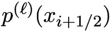 $p^{(\ell )}(x_{i + {1}/{2}})$
is third-order accurate and
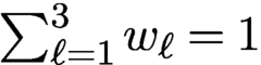 $\sum _{\ell =1}^3 w_{\ell } =1$
. However, it would be desirable if we could get higher than third-order accuracy by putting some constraints on the non-linear weights
 $w_{\ell }$
besides
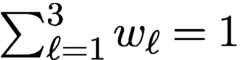 $\sum _{\ell =1}^3 w_{\ell } =1$
. Liu et al. (Reference Liu, Osher and Chan1994) developed a strategy to upgrade the order by one. Jiang and Shu (Reference Jiang and Shu1996) introduced a general framework to upgrade the order from k to
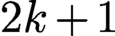 $2k+1$
. For the current
 $k=3$
case, one can find positive constants
 $\gamma _{\ell }$
, called linear weights, such that
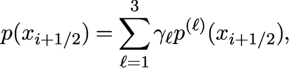 $$\begin{align*}p(x_{i + {1}/{2}}) = \sum_{\ell=1}^3 \gamma_{\ell} p^{(\ell )}(x_{i + {1}/{2}}) {,} \end{align*}$$
where
 $p(x)$
is the fourth-degree reconstruction polynomial over the big stencil
 $$ \begin{align*}S=\{ I_{i-2}, I_{i-1}, I_{i}, I_{i+1}, I_{i+2} \}, \end{align*} $$
and
 $$\begin{align*}\gamma_1 = \displaystyle \frac {1}{10},\quad \gamma_2 = \displaystyle \frac {3}{5}\quad\text{and}\quad \gamma_3 = \displaystyle \frac {3}{10}. \end{align*}$$
So if we take the non-linear weights to be equal to the linear weights
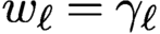 $w_{\ell } =\gamma _{\ell }$
, we would achieve fifth-order accuracy but the reconstruction would then be oscillatory near discontinuities. The idea is then to design the non-linear weights reflecting the smoothness of the function
 $u(x)$
in each of the small stencils
 $S^{(\ell )}$
, so that in the smooth case
 $w_{\ell }$
is chosen close to the linear weight
 $\gamma _{\ell }$
to secure upgraded accuracy, and near discontinuities
 $w_{\ell }$
is chosen close to zero to minimize its effect towards the WENO reconstruction. This is achieved by the so-called smoothness indicators (sometimes also called roughness indicators, perhaps more accurately), taken as
 $$ \begin{align} \beta_{\ell} = \sum_{r=1}^2 \Delta x_i^{2r-1} \int_{ x_{i-{1}/{2}}}^{ x_{i+{1}/{2}}} \biggl( \displaystyle \frac{\mathrm{d}^r}{\mathrm{d} x^r} p^{(\ell )}(x) \biggr)^2 \,\text{d} x {.} \end{align} $$
The smoothness indicator
 $\beta _{\ell }$
defined in (3.3) is a scaled square sum of the
 $L^2$
-norms of derivatives of the reconstruction polynomial
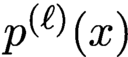 $p^{(\ell )}(x)$
over the target interval
 $I_i$
, starting from the first derivative and ending in the highest non-zero derivative of the kth-degree polynomial (here
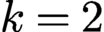 $k=2$
). The scaling factor
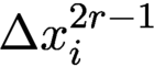 $\Delta x_i^{2r-1}$
is introduced to make the final smoothness indicator
 $\beta _{\ell }$
independent of the mesh size
 $\Delta x$
on uniform meshes (on non-uniform meshes,
 $\beta _{\ell }$
depends only on the relative ratios of mesh sizes in the stencil but is still independent of the largest mesh size
 $\Delta x$
). On uniform meshes, one can work out
 $\beta _{\ell }$
from (3.3) to get the explicit formulas
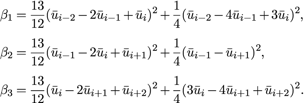 $$ \begin{align} \beta_1 &= \displaystyle \frac{13}{12} ( \bar{u}_{i-2}-2 \bar{u}_{i-1}+ \bar{u}_i )^2 +\displaystyle \frac{1}{4} ( \bar{u}_{i-2}- 4 \bar{u}_{i-1}+3 \bar{u}_i )^2 {,} \notag \\ \beta_2 &= \displaystyle \frac{13}{12} ( \bar{u}_{i-1}-2 \bar{u}_{i}+ \bar{u}_{i+1} )^2 +\displaystyle \frac{1}{4} ( \bar{u}_{i-1}- \bar{u}_{i+1} )^2 {,} \\ \beta_3 &= \displaystyle \frac{13}{12} ( \bar{u}_{i}-2 \bar{u}_{i+1}+ \bar{u}_{i+2} )^2 +\displaystyle \frac{1}{4} ( 3 \bar{u}_{i}- 4 \bar{u}_{i+1}+\bar{u}_{i+2} )^2 {.} \notag \end{align} $$
Clearly,
 $\beta _{\ell }$
are quadratic functions of the cell averages of
 $u(x)$
in the relevant stencils, which is natural from the definition (3.3). With these smoothness indicators, we define the non-linear weights as
 $$ \begin{align} w_{\ell} = \displaystyle \frac{\tilde{w}_{\ell}}{\sum_{r=1}^3 \tilde{w}_r} \quad \mbox{with}\quad \tilde{w}_r =\displaystyle \frac{\gamma_r}{(\varepsilon + \beta_r)^2} . \end{align} $$
Here
 $\varepsilon $
is a small positive number to avoid the denominator to become zero and is typically chosen as
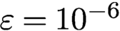 $\varepsilon = 10^{-6}$
in actual calculations. Note that when
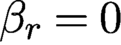 $\beta _r=0$
, the denominator of
 $\tilde {w}_r$
becomes
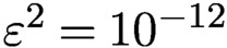 $\varepsilon ^2 = 10^{-12}$
, which is close to machine zero in double precision. With these choices of non-linear weights,
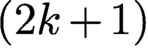 $(2k+1)$
th-order accuracy (here,
 $k=2$
, corresponding to fifth-order accuracy) can be achieved in smooth regions. Near discontinuities, that is, if one of the small stencils
 $S^{(\ell )}$
contains a discontinuity but at least one other small stencil does not contain any discontinuity, then the corresponding non-linear weight
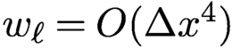 $w_{\ell } = O(\Delta x^4)$
is very small, hence the resulting WENO reconstruction is essentially non-oscillatory. Note that if all three small stencils contain a discontinuity, then all three reconstructions
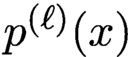 $p^{(\ell )}(x)$
are monotone in the target cell
 $I_i$
that contains this discontinuity, hence the WENO reconstruction, being a convex combination of these three reconstructions, is also essentially non-oscillatory, regardless of the values of the non-linear weights.
Higher-order (
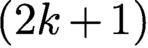 $(2k+1)$
th-order, with
 $k=3,4,5,\ldots $
) WENO reconstruction procedures were developed in Balsara and Shu (Reference Balsara and Shu2000). It appears that the fifth-, ninth- and thirteenth-order WENO schemes perform better than the third-, seventh- and eleventh-order ones (i.e. the improvement from third-order WENO to fifth-order WENO is more apparent than the improvement from fifth-order WENO to seventh-order WENO, etc.), according to extensive numerical experiments.
A similar WENO interpolation procedure extending the ENO interpolation in Section 2.1 can be defined along the same lines. We skip the details and refer the readers to Shu (Reference Shu and Cockburn1998, Reference Shu2009).
3.2 Variants of the WENO procedures
Since the publication of Liu et al. (Reference Liu, Osher and Chan1994) and Jiang and Shu (Reference Jiang and Shu1996), there have been numerous papers making modifications and improvements of the WENO procedure. However, it appears that the benefits of these modifications and improvements are not universal in all applications. We would advise a new user of WENO for solving a practical problem to use the classic fifth-order one in Jiang and Shu (Reference Jiang and Shu1996), at least at the beginning, as it is relatively simple to code and would generate stable and accurate results in most cases.
The variants of the WENO modifications and improvements will be briefly surveyed in this section. This survey is not exhaustive.
3.2.1 Improving accuracy in smooth regions
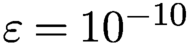
One aspect of the classical WENO schemes of Jiang and Shu (Reference Jiang and Shu1996) that could be improved is the achievable order of accuracy in smooth regions. Jiang and Shu (Reference Jiang and Shu1996) proved and numerically tested that the scheme can achieve the designed fifth-order accuracy in smooth regions, including at smooth extrema. However, Henrick, Aslam and Powers (Reference Henrick, Aslam and Powers2005) pointed out that the order of accuracy could degenerate for functions with certain types of extrema. A mapped WENO procedure, which keeps the smoothness indicator (3.3) unchanged but modifies the formula for the non-linear weights in (3.5) through a mapped function, was introduced in Henrick et al. (Reference Henrick, Aslam and Powers2005) to enhance the accuracy in such cases. However, for most test cases the degeneracy of the order of accuracy could become apparent only when
 $\varepsilon $
is taken as an extremely small number, for example
 $\varepsilon = 10^{-10}$
or even smaller, which is not necessary in practical computation. Another attempt to enhance the accuracy of the WENO procedure, termed WENO-Z, was developed in Borges, Carmona, Costa and Don (Reference Borges, Carmona, Costa and Don2008) and Castro, Costa and Don (Reference Castro, Costa and Don2011). It was based on non-linear weights that take into account the smoothness indicators of all sub-stencils in the reconstruction. Other attempts exist along similar directions and will not be discussed here.
3.2.2 Treatment of negative weights
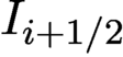
One difficulty with the classical WENO procedure of Jiang and Shu (Reference Jiang and Shu1996) is that the linear weights are uniquely determined by the accuracy requirement and can be negative, or even fail to exist. This is especially the case for WENO reconstructions, as for WENO interpolations, Carlini, Ferretti and Russo (Reference Carlini, Ferretti and Russo2005) proved that the linear weights always exist and are always positive for the procedure in Section 2.1 regardless of where in the target cell
 $I_{i+{1}/{2}}$
we are evaluating this interpolation.
If the standard WENO procedure is used when some of the linear weights are negative, for solving hyperbolic conservation laws, oscillations and instability may appear (Shi, Hu and Shu Reference Shi, Hu and Shu2002). A procedure to systematically modify the WENO procedure so that it is still stable and non-oscillatory in the presence of negative weights was developed in Shi et al. (Reference Shi, Hu and Shu2002) and has been used in many later works, for example in Qiu and Shu (Reference Qiu and Shu2002), where this technique is used to construct high-order central WENO schemes, in Puppo and Russo (Reference Puppo and Russo2006), where it is used to construct high-order staggered finite difference WENO schemes, in Castro, Gallardo and Parés (Reference Castro, Gallardo and Parés2006), where it is used to construct high-order WENO schemes for solving non-conservative hyperbolic systems, and in Noelle, Pankratz, Puppo and Natvig (Reference Noelle, Pankratz, Puppo and Natvig2006) and Xing and Shu (Reference Xing and Shu2006b, Reference Xing and Shu2006c), where it is used to construct well-balanced high-order WENO schemes for a class of balance laws including the shallow water equations.
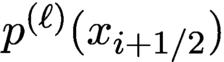
Another way to avoid this difficulty is to have only positive linear weights. For example, if we were satisfied with the WENO approximation (3.1) having the same third-order accuracy as any one of the ENO approximation
 $p^{(\ell )}(x_{i + {1}/{2}})$
, then any positive linear weights
 $\gamma _{\ell }$
, resulting in the non-linear weights
 $w_{\ell }$
(3.5) satisfying (3.2), would be fine. This approach is particularly attractive for WENO approximations on moving meshes for which the linear weights would change from different time levels, or for constructing finite volume WENO schemes on unstructured meshes; we will comment on this later in Section 3.3.
3.2.3 WENO procedures with unequal-sized sub-stencils
The classical WENO schemes in Liu et al. (Reference Liu, Osher and Chan1994), Jiang and Shu (Reference Jiang and Shu1996) and Balsara and Shu (Reference Balsara and Shu2000), as described in Section 3.2.1, use several small stencils of the same size to make up the big stencil. Another class of WENO approximations uses one large stencil and several smaller stencils. For example, one could use a big stencil,
 $$\begin{align*}S^{(1)} = \{ I_{i-2}, I_{i-1}, I_{i}, I_{i+1}, I_{i+2} \}, \end{align*}$$
and two smaller stencils,
 $$\begin{align*}S^{(2)} = \{ I_{i-1}, I_{i} \}, \quad S^{(3)} = \{ I_{i}, I_{i+1} \}, \end{align*}$$
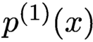
and form three reconstruction polynomials: a fourth-order
 $p^{(1)} (x)$
satisfying
 $$\begin{align*}\displaystyle \frac {1}{\Delta x_j} \int_{x_{j-{1}/{2}}}^{x_{j+{1}/{2}}} p^{(1)}(x) \,\text{d} x = \bar{u}_j, \quad j=i-2, i-1, i, i+1, i+2, \end{align*}$$
and two linear polynomials
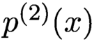 $p^{(2)}(x)$
and
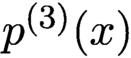 $p^{(3)}(x)$
satisfying
 $$\begin{align*}\displaystyle \frac {1}{\Delta x_j} \int_{x_{j-{1}/{2}}}^{x_{j+{1}/{2}}} p^{(2)}(x) \,\text{d} x = \bar{u}_j, \quad j=i-1, i, \end{align*}$$
and
 $$\begin{align*}\displaystyle \frac {1}{\Delta x_j} \int_{x_{j-{1}/{2}}}^{x_{j+{1}/{2}}} p^{(3)}(x) \,\text{d} x = \bar{u}_j, \quad j=i, i+1. \end{align*}$$
We then choose three arbitrary positive linear weights
 $\gamma _1$
,
 $\gamma _2$
and
 $\gamma _3$
, and use the identity
 $$\begin{align*}p^{(1)}(x) = \gamma_1 \biggl( \displaystyle \frac {1}{\gamma_1} p^{(1)}(x) - \displaystyle \frac {\gamma_2}{\gamma_1} p^{(2)}(x) - \displaystyle \frac {\gamma_3}{\gamma_1} p^{(3)}(x) \biggr) + \gamma_2 p^{(2)}(x) + \gamma_3 p^{(3)}(x) \end{align*}$$
to form our WENO approximation. If we denote
 $$\begin{align*}q^{(1)}(x) = \displaystyle \frac {1}{\gamma_1} p^{(1)}(x) - \displaystyle \frac {\gamma_2}{\gamma_1} p^{(2)}(x) - \displaystyle \frac {\gamma_3}{\gamma_1} p^{(3)}(x){,} \end{align*}$$
which is also a fourth-degree polynomial, then we can change the original high-order reconstruction on the large stencil
 $S^{(1)}$
, which is
 $$\begin{align*}p^{(1)}(x) = \gamma_1 q^{(1)}(x) + \gamma_2 p^{(2)}(x) + \gamma_3 p^{(3)}(x){,} \end{align*}$$
into a WENO reconstruction,
 $$ \begin{align} p(x) = w_1 q^{(1)}(x) + w_2 p^{(2)}(x) + w_3 p^{(3)}(x){,} \end{align} $$
with the non-linear weights
 $w_{\ell }$
computed by the same recipe (through the smoothness indicators of
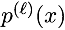 $p^{(\ell )}(x)$
) as in the regular WENO procedure detailed in Section 3.1. Because the two lower-order polynomials
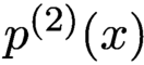 $p^{(2)}(x)$
and
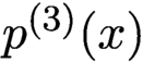 $p^{(3)}(x)$
are only second-order approximations to
 $u(x)$
, the requirement on the closeness of
 $w_{\ell }$
to the linear weights
 $\gamma _{\ell }$
in smooth regions is more stringent than that for the classical WENO schemes. Hence in practice, a procedure with enhanced accuracy such as the mapped WENO (Henrick et al. Reference Henrick, Aslam and Powers2005) or the WENO-Z (Borges et al. Reference Borges, Carmona, Costa and Don2008, Castro et al. Reference Castro, Costa and Don2011) would be preferable.
Since the linear weights can be chosen as arbitrary positive numbers, they are usually chosen in such a way that the large stencil has a relatively large linear weight like 0.8 or 0.9, and the smaller stencils share the remaining weights equally so that the total sum of the linear weights is one. Another advantage of the WENO procedure above is that the final WENO reconstruction (3.6) is a polynomial (of the same degree as the polynomial
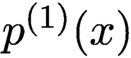 $p^{(1)}(x)$
over the large stencil) throughout the target interval
 $I_i$
, while on the other hand, the classical WENO reconstruction can only be obtained for specific points inside
 $I_i$
or for specific functionals such as the integration over the cell
 $I_i$
or the derivative at a certain point in
 $I_i$
.
The idea of the type of WENO reconstruction described above first appeared in the context of central WENO schemes, in Levy, Puppo and Russo (Reference Levy, Puppo and Russo1999, Reference Levy, Puppo and Russo2000) and Capdeville (Reference Capdeville2008). Later, Zhu and Qiu (Reference Zhu and Qiu2016, Reference Zhu and Qiu2017) constructed finite difference and finite volume WENO schemes based on this type of WENO reconstruction. More recently, Zhu and Shu (Reference Zhu and Shu2018, Reference Zhu and Shu2019, Reference Zhu and Shu2020) developed a class of multi-resolution WENO schemes based on this idea, in which all the stencils are central, and (in 1D) if the large stencil has seven cells, then the following smaller stencils have five, three and one cell(s), respectively. The multi-resolution WENO schemes are particularly attractive for unstructured meshes (Zhu and Shu Reference Zhu and Shu2019, Zhu and Shu Reference Zhu and Shu2020), because of their simplicity both in the choice of the stencil and in the freedom of arbitrary positive linear weights.
3.2.4 Hermite-type WENO procedure
If we would like to have a narrower stencil but require each cell or point to contain more than one piece of information (e.g. each cell contains the information of both its cell average and its first-order moment, or each point contains the information of both its point value and the value of the first derivative), then a high-order Hermite-type ENO or WENO polynomial can be reconstructed or interpolated in this narrower stencil. This procedure has the advantage particularly as a limiter for discontinuous Galerkin (DG) methods, to be reviewed in Section 4.3, to fit the more compact DG data structure. It can also be used as a stand-alone solver for PDEs. For more details we refer to Qiu and Shu (Reference Qiu and Shu2003b , Reference Qiu and Shu2005b , Reference Qiu and Shu2005c ).
3.3 Multi-dimensions and unstructured meshes
For tensor product-type meshes, the WENO procedure is similar to the ENO procedure as described in Section 2.5, namely either using the one-dimensional WENO approximation in a dimension-by-dimension fashion (for finite difference schemes), or using the one-dimensional WENO reconstruction first in one direction to ‘de-cell average’ in that direction, followed by the one-dimensional WENO reconstruction in the other direction to ‘de-cell average’ in the other direction.
For unstructured meshes, for example triangular meshes in two dimensions and tetrahedral meshes in three dimensions, the classical WENO procedure is quite complicated (Hu and Shu Reference Hu and Shu1999, Zhang and Shu Reference Zhang and Shu2009), aiming at using several small stencils to form a higher-order approximation from the combined large stencil at particular points (usually quadrature points along cell boundaries for evaluating numerical fluxes: see Section 4 below for more details) through linear weights, smoothness indicators and non-linear weights similar to the one-dimensional procedure. The main complication is that the linear weights are different for different quadrature points and different mesh structure, and they could easily become negative, resulting in large computational cost and the necessity to use the special treatment for negative weights (Shi et al. Reference Shi, Hu and Shu2002).
One possible remedy to reduce the computational cost of multi-dimensional WENO schemes on unstructured meshes is to relax on the achievable accuracy from the convex combination of approximations on small stencils. If we only required the same order of accuracy in the large combined stencil as that from each of the small stencils, then the choice of linear weights could be arbitrary, with the only restriction that they sum to one. This approach is particularly attractive for WENO approximations on moving meshes for which the linear weights would change from different time levels, for example in Lagrangian-type methods (Cheng and Shu Reference Cheng and Shu2008b), or for constructing finite volume WENO schemes on unstructured meshes for which linear weights are very difficult to determine, for example in Friedrichs (Reference Friedrichs1998), Dumbser and Käser (Reference Dumbser and Käser2007) and Dumbser, Käser, Titarev and Toro (Reference Dumbser, Käser, Titarev and Toro2007). It is also used in Levy, Puppo and Russo (Reference Levy, Puppo and Russo1999) to construct high-order central WENO schemes, for which the linear weights might fail to exist for some cases if we were to insist on the maximum attainable order of accuracy. Liu and Zhang (Reference Liu and Zhang2013) combined this approach with the classical WENO procedure of Zhang and Shu (Reference Zhang and Shu2009) to obtain more robust and less expensive WENO schemes on three-dimensional tetrahedra.
The procedure of using stencils with different sizes to form WENO approximations, which allows the choice of linear weights to be arbitrary with the only restriction that they sum to one, as described in Section 3.2.3, is a better choice for constructing WENO approximations on unstructured meshes or on moving meshes. These WENO approximations are not only easy to construct: they also provide a polynomial in the target cell, rather than just individual approximations at different quadrature points from the classical WENO procedure. We would advocate in particular the multi-resolution WENO schemes developed in Zhu and Shu (Reference Zhu and Shu2019, Reference Zhu and Shu2020), which have provided a simple and effective WENO approximation procedure for both two- and three-dimensional unstructured meshes.
For more details about the two- (and higher-) dimensional WENO reconstruction procedures, we again refer to the references listed above and to Shu (Reference Shu and Cockburn1998).
3.4 Other WENO procedures
The WENO interpolation and reconstruction procedures described in previous sections are the most commonly used WENO procedures in applications. However, other WENO procedures can be similarly defined.
3.4.1 WENO approximations to derivatives
We could use WENO interpolation to approximate the first-, second- or higher-order derivatives of the piecewise smooth function
 $u(x)$
, given its point values
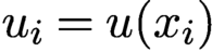 $u_i=u(x_i)$
. By the classical WENO procedure, this would involve different linear weights from those for interpolation, which could often become negative (Liu, Shu and Zhang Reference Liu, Shu and Zhang2009b
, Reference Liu, Shu and Zhang2011b
), hence requiring the special treatment for negative weights (Shi et al. Reference Shi, Hu and Shu2002). Another point requiring particular attention is that in the definition of the smoothness indicator (3.3), the summation should start from
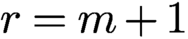 $r=m+1$
for approximating an mth-order derivative, since one should not include the mth-order derivative itself in the measurement of smoothness indicator if one is approximating the mth-order derivative. This is a common mistake which may cause poor performance both in accuracy loss and in spurious oscillations.
The procedure of using stencils with different sizes to form WENO approximations, which allows the choice of linear weights to be arbitrary with the only restriction that they sum to one, as described in Section 3.2.3, is a good choice for constructing WENO approximations to derivatives of different orders. Since the resulting WENO approximation is a polynomial in the target cell, the approximation to the mth derivatives can be readily obtained just by taking the mth derivative of the WENO polynomial, paying attention only in the computation of the smoothness indicator (3.3), whose summation must start from
 $r=m+1$
. We would again advocate in particular the multi-resolution WENO procedure developed in Zhu and Shu (Reference Zhu and Shu2018, Reference Zhu and Shu2019, Reference Zhu and Shu2020) for this purpose.
3.4.2 WENO approximations to integration
We could use WENO interpolation to approximate the integration of the piecewise smooth function
 $u(x)$
over the target cell, given its point values
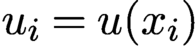 $u_i=u(x_i)$
. By the classical WENO procedure, this would again involve different linear weights from those for interpolation, which could often become negative (Shu Reference Shu2009, Chou and Shu Reference Chou and Shu2006, Chou and Shu Reference Chou and Shu2007), hence requiring the special treatment for negative weights (Shi et al. Reference Shi, Hu and Shu2002). Once more, the procedure of using stencils with different sizes to form WENO approximations, which allows the choice of linear weights to be arbitrary with the only restriction that they sum to one, as described in Section 3.2.3, is a good choice for constructing WENO integration. Since the resulting WENO approximation is a polynomial in the target cell, the approximation to the integration over the target cell can be readily obtained just by taking the integration of the WENO polynomial. We would once more advocate in particular the multi-resolution WENO procedure developed in Zhu and Shu (Reference Zhu and Shu2018, Reference Zhu and Shu2019, Reference Zhu and Shu2020) for this purpose.
4 ENO and WENO schemes for conservation laws
The most important application of the ENO and WENO approximation procedure outlined in Sections 2 and 3 is to perform spatial discretizations for solving the hyperbolic conservation laws (1.1), Hamilton–Jacobi equations (1.2) or convection–diffusion equations (1.3). In this section we describe the procedure for solving hyperbolic conservation laws.
4.1 Finite volume schemes for conservation laws
One of the most important classes of numerical schemes for solving hyperbolic conservation laws is the class of finite volume schemes. We will describe ENO and WENO finite volume schemes in this subsection.
4.1.1 One-dimensional scalar equations
If we integrate the conservation law (1.1) over the cell
 $I_i = (x_{i- {1}/{2}}, x_{i+ {1}/{2}})$
, we obtain its integral form
 $$ \begin{align} \displaystyle \frac{\mathrm{d}}{\mathrm{d} t} \bar{u}_i + \displaystyle \frac{1}{\Delta x_i} ( f(u_{i+ {1}/{2}}) - f(u_{i- {1}/{2}}) ) = 0 {,} \end{align} $$
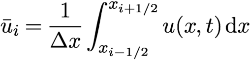
where
 $$\begin{align*}\bar{u}_i = \displaystyle \frac{1}{\Delta x} \int_{x_{i-{1}/{2}}}^{x_{i+{1}/{2}}} u(x,\,t) \,\text{d} x \end{align*}$$
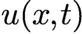
is the spatial cell average of the solution
 $u(x,t)$
in the cell
 $I_i$
as defined in Section 2.2. To convert the equality (4.1) into a finite volume scheme, we would take our computational variables as the cell averages
 $ \{ \bar {u}_i \}$
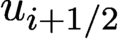
and use the ENO or WENO reconstruction procedures described in Sections 2.2 or 3.1 respectively, to obtain an approximation to the point values
 $u_{i+ {1}/{2}}$
. For the purpose of stability, we actually compute two reconstructed values
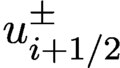 $u^{\pm }_{i+ {1}/{2}}$
, corresponding to the ENO or WENO approximations (which are piecewise polynomials) in the cell
 $I_i$
and in the cell
 $I_{i+1}$
respectively. We can then feed them into a numerical flux,
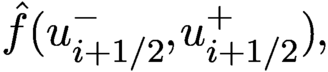 $$\begin{align*}\hat{f} ( u_{i+{1}/{2}}^-, u_{i+{1}/{2}}^+ ){,} \end{align*}$$
to obtain the semi-discrete finite volume scheme
 $$ \begin{align} \displaystyle \frac{\mathrm{d}}{\mathrm{d} t} \bar{u}_i = - \displaystyle \frac{1}{\Delta x_i} [ \hat{f} ( u^-_{i+{1}/{2}}, u^+_{i+{1}/{2}} ) - \hat{f} ( u^-_{i-{1}/{2}}, u^+_{i-{1}/{2}} ) ] . \end{align} $$
The choice of the numerical flux
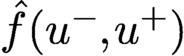 $\hat {f}(u^-, u^+)$
is based on exact or approximate Riemann solvers. In the scalar case they are chosen from the class of monotone fluxes. Examples of monotone fluxes include the Godunov flux, the Engquist–Osher flux and the Lax–Friedrichs flux. We refer to LeVeque (Reference LeVeque1990) and references therein for a detailed discussion of monotone fluxes.
The ENO reconstruction procedure to obtain
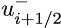 $u_{i+{1}/{2}}^-$
starts with the cell
 $I_i$
in the stencil, then adding one cell at a time with the ENO process until the desired number of cells is reached, as outlined in Section 2.2. The ENO reconstruction procedure to obtain
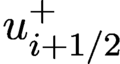 $u_{i+{1}/{2}}^+$
is mirror symmetric (with respect to the location
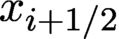 $x_{i+{1}/{2}}$
), namely starting with the cell
 $I_{i+1}$
in the stencil, and then adding one cell at a time with the ENO process until the desired number of cells is reached.
Likewise, the WENO reconstruction procedure to obtain
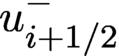 $u_{i+{1}/{2}}^-$
uses a left-biased stencil, for example
 $\{ I_{i-2}, I_{i-1}, I_{i}, I_{i+1}, I_{i+2} \}$
in the fifth-order case, and the WENO procedure as outlined in Section 3.1. The WENO reconstruction procedure to obtain
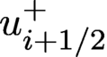 $u_{i+{1}/{2}}^+$
is mirror symmetric (with respect to the location
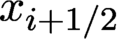 $x_{i+{1}/{2}}$
), namely using a right-biased stencil, for example
 $\{ I_{i-1}, I_{i}, I_{i+1}, I_{i+2}, I_{i+3} \}$
in the fifth-order case, and the WENO procedure.
Note that the mesh for the finite volume scheme can be non-uniform, and also the numerical flux
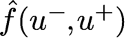 $\hat {f}(u^-, u^+)$
only needs to be a Lipschitz-continuous function with respect to
 $u^-$
and
 $u^+$
, and thus many less smooth fluxes such as the Godunov flux or the Roe flux could be used. We again refer to LeVeque (Reference LeVeque1990) and references therein for a detailed discussion of these fluxes.
4.1.2 One-dimensional systems
For a one-dimensional conservation law system (1.1), u is a vector and
 $f(u)$
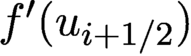
is a vector function. There is a requirement that the Jacobian matrix
 $f'(u)$
is diagonalizable, with only real eigenvalues and a complete set of eigenvectors. Let us assume that
 $R(u)$
consists of the right eigenvectors of
 $f'(u)$
as its columns, hence
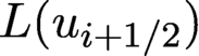
 $L(u)=R^{-1}(u)$
exists (which actually consists of the left eigenvectors of
 $f'(u)$
as its rows). We also denote the diagonal matrix
 $\Lambda (u)$
which contains the eigenvalues of
 $f'(u)$
in its diagonal line, then we have
 $f'(u) R(u) = R(u) \Lambda (u)$
, or
 $L(u) f'(u) R(u) = \Lambda (u)$
.
The ENO or WENO finite volume scheme is still (4.2). The numerical flux
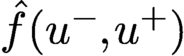 $\hat {f}(u^-, u^+)$
could be based on exact or approximate Riemann solvers. Typical choices include the Godunov flux, the Lax–Friedrichs flux, the Roe flux and the HLLC flux. We refer to LeVeque (Reference LeVeque1990) and Toro (Reference Toro1997) for more details of Riemann solvers and numerical fluxes for the system case.
As to the reconstruction to obtain
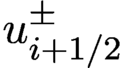 $u_{i+{1}/{2}}^{\pm }$
from the cell averages
 $\bar {u}_j$
, we could perform the ENO or WENO reconstruction procedure on each component of the vector
 $\bar {u}_j$
, then it would just be using the scalar reconstruction algorithm m times for each of the m components of the vector
 $\bar {u}_j$
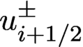
. This would produce satisfactory results for many test cases, with smooth solutions or with solutions of weak shocks. However, for problems with strong shocks, especially for problems with multiple discontinuities (such as a shock and a contact discontinuity) resulting from a single discontinuity initially (this would be the case for many Riemann problems), the component-wise ENO or WENO reconstruction could lead to spurious oscillations. A more robust, albeit more expensive, way to perform the reconstruction is to perform it in the local characteristic directions, which is summarized below. To obtain the approximation
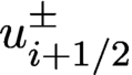
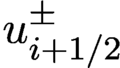
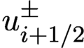 $u_{i+{1}/{2}}^{\pm }$
, we have the following steps.
-
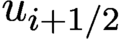
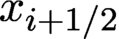
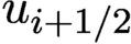
(1) Determine an approximate mid-point value of u at
$x_{i+{1}/{2}}$
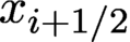
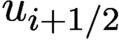
, denoted by
$u_{i+{1}/{2}}$
. Do not confuse this with the final reconstruction values
$u_{i+{1}/{2}}^{\pm }$
. This approximate mid-point value
$u_{i+{1}/{2}}$
is used only as a reference to perform local characteristic decompositions, hence it does not need to be a high-order approximation of u at
$x_{i+{1}/{2}}$
. Most often, we will take the so-called Roe average between
$\bar {u}_i$
and
$\bar {u}_{i+1}$
(Roe Reference Roe1978) as
$u_{i+{1}/{2}}$
. When the Roe average is not available, we could simply choose the arithmetic mean
$u_{i+{1}/{2}} = \tfrac {1}{2} (\bar {u}_i + \bar {u}_{i+1})$
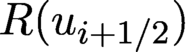
. We denote the right eigenvector matrix
$R(u_{i+{1}/{2}})$
and the left eigenvector matrix
$L(u_{i+{1}/{2}})$
of the Jacobian matrix
$f'(u_{i+{1}/{2}})$
as R and L below. This will not cause confusion since all the steps here are used to compute
$u_{i+{1}/{2}}^{\pm }$
for fixed i. -
(2) Project all the cell averages needed in the ENO or WENO procedure to compute
$u_{i+{1}/{2}}^{\pm }$
into the characteristic fields determined by R and L. For example, if we perform a fifth-order WENO reconstruction to get
$u_{i+{1}/{2}}^{\pm }$
, we would need to calculate
$$\begin{align*}\bar{v}_j = L \bar{u}_j, \quad j=i-2, i-1, i, i+1, i+2, i+3 . \end{align*}$$
-
(3) Perform the scalar ENO or WENO reconstruction procedure on each component of
$\bar {v}_j$
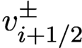
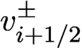
, to obtain
$v_{i+{1}/{2}}^{\pm }$
. -
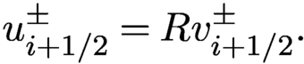
(4) Project
$v_{i+{1}/{2}}^{\pm }$
back to the original vector space,
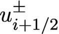
$$\begin{align*}u_{i+{1}/{2}}^{\pm} = R v_{i+{1}/{2}}^{\pm} . \end{align*}$$





4.1.3 Multi-dimensional problems
For a multi-dimensional conservation law
 $$ \begin{align} u_t + \nabla \cdot f(u) = 0 , \end{align} $$
a finite volume scheme approximates its integrated version
 $$ \begin{align} \bar{u}_i + \displaystyle \frac {1}{|\Delta_i|} \int_{\partial \Delta_i} f(u) \cdot n \,\text{d} s = 0 , \end{align} $$
where
 $\Delta _i$
is a cell (e.g. a rectangle or triangle in 2D),
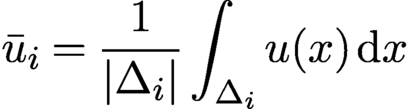 $$\begin{align*}\bar{u}_i = \displaystyle \frac {1}{|\Delta_i|} \int_{\Delta_i} u(x) \,\text{d} x \end{align*}$$
is the cell average of u in the cell
 $\Delta _i$
,
 $|\Delta _i|$
is the size of the cell
 $\Delta _i$
(area in 2D and volume in 3D),
 $\partial \Delta _i$
is the boundary of the cell
 $\Delta _i$
(edges in 2D and surfaces in 3D), and n is the outward unit normal along
 $\partial \Delta _i$
. The integrated version (4.4) can be obtained from the PDE (4.3) by integrating over the cell
 $\Delta _i$
and using the divergence theorem. To convert the integrated version (4.4), which is satisfied by the exact solution of the PDE (4.3), into a finite volume scheme, we would take our computational variables as the cell averages
 $ \{ \bar {u}_i \}$
. The integrals along the boundary of the cell
 $\partial \Delta _i$
in (4.4) are replaced by their quadrature numerical integrations (typically, Gaussian quadrature rules are used if possible), and the physical flux
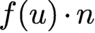 $f(u) \cdot n$
is replaced by a one-dimensional numerical flux
 $\hat {g} (u^{\text {int}(D_i)}, u^{\text {ext}(D_i)})$
, where
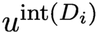 $u^{\text {int}(D_i)}$
and
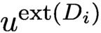 $u^{\text {ext}(D_i)}$
refer to numerical approximations of the point value u at the quadrature point inside the cell
 $D_i$
and outside the cell
 $D_i$
(hence inside the neighbouring cell), respectively. The one-dimensional numerical flux
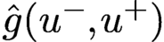 $\hat {g} (u^-, u^+)$
is the same as those discussed in the one-dimensional case in Sections 4.1.1 and 4.1.2 respectively. Finally, we obtain the point values
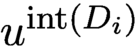 $u^{\text {int}(D_i)}$
and
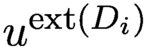 $u^{\text {ext}(D_i)}$
from the cell averages
 $\bar {u}_j$
by a multi-dimensional ENO or WENO reconstruction procedure, the two-dimensional versions having been described in Section 3.3. For the system case, we can carry out a similar reconstruction in the local characteristic fields, determined by the Jacobian matrix of the one-dimensional physical flux
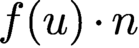 $f(u) \cdot n$
.
4.2 Finite difference schemes for conservation laws
Different from finite volume schemes which use cell averages as the computational variables, finite difference schemes use point values as the computational variables. We will describe conservative ENO and WENO finite difference schemes below.
4.2.1 One-dimensional scalar equations
We use
 $x_i$
to denote a uniform mesh point and
 $u_i$
to denote the numerical approximation of
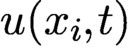 $u(x_i,t)$
. Unlike finite volume schemes, which can be applied to any non-uniform meshes, the conservative finite difference scheme of order at least three can only be designed for uniform of smooth meshes. We will assume the mesh is uniform for simplicity, hence
 $\Delta x=x_{i+1}-x_i$
is a constant. The conservative finite difference scheme approximating (1.1) is of the form
 $$ \begin{align} \displaystyle \frac{\mathrm{d}}{\mathrm{d} t} {u}_i + \displaystyle \frac{1}{\Delta x} ( \hat{f}_{i+ {1}/{2}} - \hat{f}_{i- {1}/{2}} ) = 0 {,} \end{align} $$
where
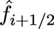 $\hat {f}_{i+ {1}/{2}}$
is a numerical flux which depends on several neighbouring point values; for example, for a fifth-order WENO scheme, it depends on
 $u_{i-2}$
,
 $u_{i-1}$
,
 $u_{i}$
,
 $u_{i+1}$
,
 $u_{i+2}$
and
 $u_{i+3}$
. Superficially, the finite difference scheme (4.5) seems to be totally different from the finite volume scheme (4.2). However, the following simple lemma by Shu and Osher (Reference Shu and Osher1989) sets up a direct link between these two types of schemes.
Lemma. If
 $h(x) = h_{\Delta x}(x)$
is implicitly defined as
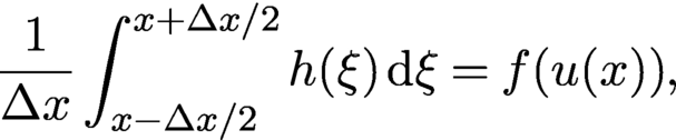 $$ \begin{align} \displaystyle \frac {1}{\Delta x} \int_{x-{\Delta x}/{2}}^{x+{\Delta x}/{2}} h(\xi ) \,\text{d} \xi = f(u(x)){,} \end{align} $$
then
 $$\begin{align*}\displaystyle \frac{1}{\Delta x} ( h(x_{i+{1}/{2}}) - h(x_{i-{1}/{2}}) ) = f(u)_x |_{x=x_i} . \end{align*}$$
The proof is straightforward: just take an x derivative on both sides of (4.6) and evaluate the results at
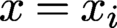 $x=x_i$
.
This simple lemma allows us to take the numerical flux in the finite difference scheme (4.5) as
 $$ \begin{align} \hat{f}_{i+{1}/{2}} = h(x_{i+{1}/{2}}) \end{align} $$
to ensure rth-order accuracy, if the function
 $h(x)$
in the lemma can be computed to rth-order accuracy.
Of course, the issue seems to remain as how to compute a good approximation to
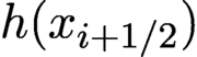 $h(x_{i+{1}/{2}})$
. Note that the definition (4.6) of
 $h(x)$
implies that
 $$\begin{align*}\bar{h}_i \equiv \displaystyle \frac {1}{\Delta x} \int_{x_{i-{1}/{2}}}^{x_{i+{1}/{2}}} h(\xi ) \,\text{d} \xi = f(u_i) , \end{align*}$$
which is known for a finite difference scheme, since the point values
 $u_i$
are the computational variables. Therefore, we are given the cell averages
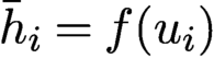 $\bar {h}_i=f(u_i)$
of the function
 $h(x)$
and we would need to approximate its point values
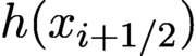 $h(x_{i+{1}/{2}})$
to high-order accuracy to obtain the numerical flux
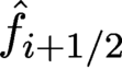 $\hat {f}_{i+{1}/{2}}$
in (4.7). This is exactly the reconstruction problem that we discussed in Section 2.2. Hence we can use the same ENO or WENO reconstruction procedure discussed in Section 2.2 or Section 3.1, which has been used for finite volume schemes in the previous sections. This implies that a finite difference ENO or WENO code for the scalar one-dimensional conservation law (1.1) shares the main reconstruction subroutine with a finite volume ENO or WENO code. The only difference is the input–output pair: for a finite volume scheme, the input is the set of cell averages
 $\{ \bar {u}_i \}$
and the output is the reconstructed values of the solution at the cell interfaces
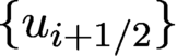 $\{ u_{i+ {1}/{2}} \}$
; for a finite difference scheme, the input is the set of the point values of the physical flux
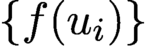 $\{ f(u_i) \}$
and the output is the numerical fluxes at the cell interfaces
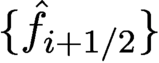 $\{ \hat {f}_{i+{1}/{2}} \}$
.
Another issue for finite difference schemes is the way to ensure upwinding and stability. For this purpose, the finite difference procedure described above is applied to
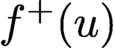 $f^+(u)$
and
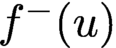 $f^-(u)$
separately, where
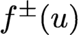 $f^{\pm } (u)$
correspond to a flux splitting
 $$ \begin{align} f(u) = f^+(u) + f^-(u) \end{align} $$
with
 $$ \begin{align} \displaystyle \frac{\mathrm{d}}{\mathrm{d} u} f^+(u) \geq 0, \quad \displaystyle \frac{\mathrm{d}}{\mathrm{d} u} f^-(u) \leq 0 . \end{align} $$
The reconstruction for
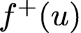 $f^+(u)$
uses a biased stencil with one more point to the left, and that for
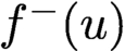 $f^-(u)$
uses a biased stencil with one more point to the right, to obey correct upwinding. For ENO schemes, the stencil choice to evaluate
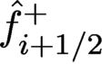 $\hat {f}^+_{i+{1}/{2}}$
starts with a single point
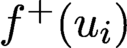 $f^+(u_i)$
in the stencil, and then adding one point at a time by the ENO process until the desired number of points is reached, while the stencil choice to evaluate
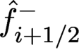 $\hat {f}^-_{i+{1}/{2}}$
starts with a single point
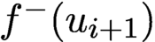 $f^-(u_{i+1})$
in the stencil, and then adding one point at a time by the ENO process until the desired number of points is reached. For the fifth-order WENO schemes, the big stencil for reconstructing
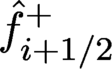 $\hat {f}^+_{i+{1}/{2}}$
contains
 $$\begin{align*}\{ f^+(u_{i-2}), f^+(u_{i-1}), f^+(u_{i}), f^+(u_{i+1}), f^+(u_{i+2}) \}, \end{align*}$$
and the big stencil for reconstructing
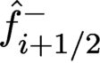 $\hat {f}^-_{i+{1}/{2}}$
contains
 $$\begin{align*}\{ f^-(u_{i-1}), f^-(u_{i}), f^-(u_{i+1}), f^-(u_{i+2}), f^-(u_{i+3}) \}. \end{align*}$$
We would also require that
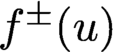 $f^{\pm } (u)$
are smooth functions of u. The most commonly used flux splitting is the Lax–Friedrichs splitting
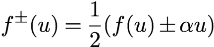 $$\begin{align*}f^{\pm} (u) = \displaystyle \frac 12 ( f(u) \pm \alpha u ) \end{align*}$$
with
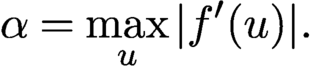 $$\begin{align*}\alpha = \max_u |f'(u)|. \end{align*}$$
We remark that for any flux splitting (4.8) satisfying (4.9),
 $\hat {f}(u^-, u^+) = f^+ (u^-) + f^- (u^+)$
is a monotone flux in the scalar case.
An alternative formulation of the finite difference flux
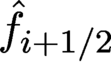 $\hat {f}_{i+{1}/{2}}$
is based on ENO or WENO interpolation, not reconstruction, but with more complicated formulas involving not only the point values from the interpolation, but also all the even-order derivatives of the flux function (Shu and Osher Reference Shu and Osher1988, Jiang, Shu and Zhang Reference Jiang, Shu and Zhang2013). One advantage of this alternative formulation is that it allows use of all monotone fluxes, regardless of their smoothness. Other advantages will be commented upon in later sections.
4.2.2 One-dimensional systems
Similar to finite volume schemes, the conservative finite difference ENO or WENO scheme for one-dimensional systems is almost the same as that for the scalar case. The only exception is the reconstruction on local characteristic field. If this is needed, it is performed in the same way as that for finite volume schemes, as described in Section 4.1.2.
4.2.3 Multi-dimensional problems
A major advantage of finite difference schemes over finite volume schemes is the efficiency in multi-dimensions. Conservative finite difference schemes of order higher than two can only be defined on uniform tensor product or smooth curvilinear meshes. We use two-dimensional tensor product uniform meshes as an example. We have a mesh
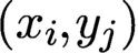 $(x_i, y_j)$
where
 $\Delta x = x_{i+1} - x_i$
and
 $\Delta y = y_{j+1} - y_j$
are both constants. A finite difference scheme approximates the PDE form (4.3) directly and can proceed dimension by dimension. The scheme is
 $$\begin{align*}\displaystyle \frac {\mathrm{d} u_{ij}(t)}{\mathrm{d} t} = -\displaystyle \frac {1}{\Delta x}(\hat{f}_{i+{1}/{2} ,j}-\hat{f}_{i-{1}/{2} ,j}) -\displaystyle \frac {1}{\Delta y}(\hat{g}_{i,j+{1}/{2}}-\hat{g}_{i,j-{1}/{2}}) {,} \end{align*}$$
where the numerical flux
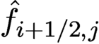 $\hat {f}_{i+{1}/{2} ,j}$
can be computed from
 $ \{ u_{ij} \}$
with fixed j in exactly the same way as in the one-dimensional case described in Section 4.2.1; likewise for
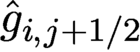 $\hat {g}_{i,j+{1}/{2}}$
. Therefore, the computational cost is exactly the same as in the one-dimensional case per point per direction. This is much more efficient than finite volume schemes. We refer to Casper, Shu and Atkins (Reference Casper, Shu and Atkins1994) for a comparison of finite difference and finite volume ENO schemes.
4.2.4 Weighted compact schemes
To get better wave resolution capability with a (nominally) narrower stencil, we could use the so-called compact schemes (Lele Reference Lele1992). However, for solutions with strong shocks, the compact schemes could also generate spurious oscillations. To overcome this difficulty, hybrid compact-ENO or compact-WENO schemes and weighted compact schemes were designed, for example in Adams and Shariff (Reference Adams and Shariff1996), Mahesh, Lele and Moin (Reference Mahesh, Lele and Moin1997), Deng and Maekawa (Reference Deng and Maekawa1997), Deng and Zhang (Reference Deng and Zhang2000), Jiang, Shan and Liu (Reference Jiang, Shan and Liu2001) and Zhang, Jiang and Shu (Reference Zhang, Jiang and Shu2008).
4.3 WENO reconstruction as a limiter for discontinuous Galerkin methods
Discontinuous Galerkin (DG) methods, especially the Runge–Kutta DG (RKDG) methods (Cockburn and Shu Reference Cockburn and Shu1989, Reference Cockburn and Shu1998, Reference Cockburn and Shu2001), are also a popular class of methods for solving hyperbolic conservation laws and general convection-dominated convection–diffusion equations, especially for unstructured meshes in multi-dimensions. The algorithm formulation of the RKDG methods is very similar to that of finite volume methods, except that the RKDG methods do not have a reconstruction step to reconstruct the piecewise polynomial solution from the cell averages: rather, they evolve the whole polynomial solution in time. As such, the RKDG methods may suffer from spurious oscillations or even non-linear instability when the solution contains strong shocks. One possible way to remedy this is to apply a non-linear limiter, that is, to modify the DG solution in the so-called ‘troubled cells’ to another polynomial of the same degree, which is less oscillatory, and is hopefully also as high-order accurate as the original DG polynomial in case the ‘troubled cell’ turns out to be a smooth cell of the solution (although there are numerous papers on the choice of troubled cell indicators (Qiu and Shu Reference Qiu and Shu2005a), none of them is bullet-proof in selecting all and only shocked cells, especially in coarser meshes, so we must assume that the troubled cell indicator could mistakenly identify a good, smooth cell as a troubled cell).
The WENO reconstruction would serve as a good limiter for RKDG schemes in troubled cells, as it could maintain the original high-order accuracy if mistakenly used in smooth cells, and it can keep the cell average unchanged, hence ensuring conservation. Earlier WENO limiters for RKDG schemes (Qiu and Shu Reference Qiu and Shu2003b, Reference Qiu and Shu2005b, Reference Qiu and Shu2005d) used wider stencils than the original communication structure of DG methods (the DG methods only communicate with immediate neighbouring cells via numerical fluxes), so they have problems in the original DG code structure, especially for parallel implementations. Subsequently more compact WENO limiters were designed (Zhong and Shu Reference Zhong and Shu2013, Zhu, Zhong, Shu and Qiu Reference Zhu and Qiu2017), which use only the information from immediate neighbouring cells. We mention in particular the compact WENO limiters recently developed by Zhu, Qiu and Shu (Reference Zhu, Qiu and Shu2020), based on the multi-resolution WENO procedure of Zhu and Shu (Reference Zhu and Shu2018, Reference Zhu and Shu2019), which appear to be quite robust for RKDG methods of various orders.
5 ENO and WENO schemes for Hamilton–Jacobi equations
In the one-dimensional case, the conservation law equation (1.1) and the Hamilton–Jacobi equation (1.2) are equivalent, if we identify
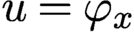 $u=\varphi _x$
. The entropy solution u of (1.1) corresponds to the viscosity solution
 $\varphi $
of (1.2) with
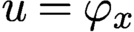 $u=\varphi _x$
. Therefore, successful ENO and WENO algorithms for solving conservation laws discussed in the previous sections can be easily adapted to solve Hamilton–Jacobi equations. Note that there is no advantage in using finite volume schemes (those evolving the cell averages of
 $\varphi $
) for Hamilton–Jacobi equations, as finite difference schemes (those evolving the point values of
 $\varphi $
) can handle non-uniform meshes and unstructured meshes well and are simpler to design than finite volume schemes.
In one space dimension, the finite difference ENO or WENO schemes for solving the Hamilton–Jacobi equation (1.2) take the form
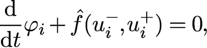 $$ \begin{align} \displaystyle \frac{\mathrm{d}}{\mathrm{d} t} \varphi_{i} + \hat{f} (u^-_{i}, u^+_{i}) = 0 {,} \end{align} $$
where
 $\varphi _{i}$
is the approximation to the point value
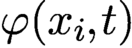 $\varphi (x_i,t)$
,
 $u^{\pm }$
are the approximations to the derivative
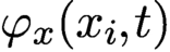 $\varphi _x(x_i,t)$
with stencils biased to the right and to the left, respectively, and
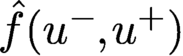 $\hat {f} (u^-, u^+)$
is a monotone Hamiltonian, which is the same as a monotone flux for the conservation law case. To obtain
 $u^{\pm }_{i}$
in (5.1), we use the ENO or WENO approximations to the first derivative of
 $\varphi $
at the point
 $x_i$
, as described in Section 3.4.1. For ENO, the approximation of
 $u^-_i$
starts with a stencil containing the two points
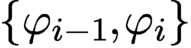 $\{ \varphi _{i-1}, \varphi _{i} \}$
and then with one point added to the stencil at each step in the ENO fashion, until the desired number of points is reached, while the approximation of
 $u^+_i$
starts with a stencil containing the two points
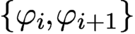 $\{ \varphi _{i}, \varphi _{i+1} \}$
and then with one point added to the stencil at each step in the ENO fashion, until the desired number of points is reached. For the fifth-order WENO, the stencil for the approximation of
 $u^-_i$
is
 $\{ \varphi _{i-3}, \varphi _{i-2}, \varphi _{i-1}, \varphi _{i}, \varphi _{i+1}, \varphi _{i+2} \}$
, while the stencil for the approximation of
 $u^+_i$
is
 $\{ \varphi _{i-2}, \varphi _{i-1}, \varphi _{i}, \varphi _{i+1}, \varphi _{i+2}, \varphi _{i+3} \}$
.
For multi-dimensional Hamilton–Jacobi equations, for example the two-dimensional version
 $$ \begin{align} \varphi_t + f(\varphi_x, \varphi_y) =0 , \end{align} $$
the ENO and WENO schemes still follow a similar framework. For tensor product meshes, which are not necessarily uniform, we can obtain the finite difference scheme in the form
 $$ \begin{align} \displaystyle \frac{\mathrm{d}}{\mathrm{d} t} \varphi_{i,j} + \hat{f} (u^-_{i,j}, u^+_{i,j}; v^-_{i,j}, v^+_{i,j}) = 0{,} \end{align} $$
where
 $\varphi _{i,j}$
is the approximation to the point value
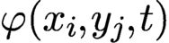 $\varphi (x_i,y_j,t)$
,
 $u^{\pm }$
are the approximations to the derivative
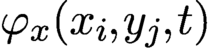 $\varphi _x(x_i,y_j,t)$
with stencils biased to the right and to the left, respectively,
 $v^{\pm }$
are the approximations to the derivative
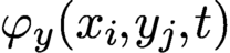 $\varphi _y(x_i,y_j,t)$
with stencils biased to the top and to the bottom, respectively, and
 $\hat {f} (u^-, u^+; v^-, v^+)$
is a monotone Hamiltonian. We refer to Crandall and Lions (Reference Crandall and Lions1984), Osher and Sethian (Reference Osher and Sethian1988) and Osher and Shu (Reference Osher and Shu1991) for examples of two-dimensional monotone Hamiltonians. The ENO and WENO approximations to obtain
 $u^{\pm }_{i,j}$
are identical to the one-dimensional case in the x-variable, with the index j fixed; likewise for
 $v^{\pm }_{i,j}$
. For unstructured meshes, we refer to Abgrall (Reference Abgrall1996) for the construction of monotone Hamiltonians, and to Zhang and Shu (Reference Zhang and Shu2003) for high-order WENO schemes. We also have Hermite-type WENO schemes designed for solving Hamilton–Jacobi equations, for example in Qiu and Shu (Reference Qiu and Shu2005c) and Zheng, Shu and Qiu (Reference Zhu and Qiu2017, Reference Zhu and Shu2017). We refer to Osher and Sethian (Reference Osher and Sethian1988), Osher and Shu (Reference Osher and Shu1991), Jiang and Peng (Reference Jiang and Peng2000) and Shu (Reference Shu and Goh2007) for more details on ENO and WENO schemes for solving Hamilton–Jacobi equations.
6 ENO and WENO schemes for convection–diffusion equations
For the convection–diffusion equation (1.3), the simplest method is to use ENO or WENO approximations described in previous sections to discretize the convection term
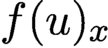 $f(u)_x$
, and then use central difference approximations of a suitable order of accuracy to discretize the diffusion term
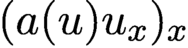 $(a(u) u_x)_x$
. This procedure works fine for most cases, except for the case with degenerate diffusion terms, that is,
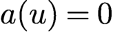 $a(u)=0$
at certain values of u. Degenerate diffusion terms could lead to hyperbolic-like features in the solutions, such as discontinuous derivatives or even discontinuities in the solutions themselves. In such cases, it would be prudent to also use ENO or WENO approximations to treat the diffusion term
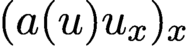 $(a(u) u_x)_x$
. The procedure is similar to that for the convection term, with some difference in the design of smoothness indicators, etc. We refer to Liu, Shu and Zhang (Reference Liu, Shu and Zhang2011b) for more detailed discussions.
7 Time discretizations
Up to now, we have only discussed spatial discretizations using ENO or WENO procedures. In practice, we would certainly also need to discretize the time variable. The simplest and perhaps most widely used approach is to adopt the explicit total variation diminishing (TVD) discretization (Shu and Osher 1988, Shu Reference Shu1988), also called the strong stability preserving (SSP) (Gottlieb, Shu and Tadmor Reference Gottlieb, Shu and Tadmor2001), Runge–Kutta or multi-step time discretization, which would preserve stability in any norm, semi-norm or convex functional enjoyed by the first-order Euler forward time discretization. The most popular one in this class is the third-order TVD or SSP time discretization (Shu and Osher Reference Shu1988):
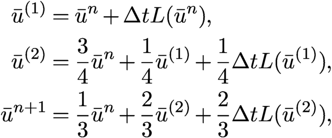 $$ \begin{align} \bar{u}^{(1)} &= \bar{u}^n + \Delta t L( \bar{u}^n){,} \notag \\ \bar{u}^{(2)} &= \displaystyle \frac{3}{4} \bar{u}^n +\displaystyle \frac{1}{4} \bar{u}^{(1)} + \displaystyle \frac{1}{4} \Delta t L( \bar{u}^{(1)} ){,} \\ \bar{u}^{n+1} &= \displaystyle \frac{1}{3} \bar{u}^n +\displaystyle \frac{2}{3} \bar{u}^{(2)} + \displaystyle \frac{2}{3} \Delta t L( \bar{u}^{(2)} ){,} \notag \end{align} $$
where
 $L(u)$
is the spatial discretization operator. We refer to Gottlieb et al. (Reference Gottlieb, Shu and Tadmor2001) and Gottlieb, Ketcheson and Shu (Reference Gottlieb, Ketcheson and Shu2009, Reference Gottlieb, Ketcheson and Shu2011) for more details of the TVD or SSP time discretizations.
An alternative method of time discretization is via the Lax–Wendroff procedure, namely performing a Taylor expansion in time and converting all time derivatives to spatial derivatives by repeatedly using the PDE, and finally discretizing all the spatial derivatives to the correct order of accuracy. The ADER schemes and GRP schemes also belong to this class. See, for example, Harten et al. (Reference Harten, Engquist, Osher and Chakravarthy1987), Titarev and Toro (Reference Titarev and Toro2005), Ben-Artzi, Li and Warnecke (Reference Ben-Artzi, Li and Warnecke2006) and Qiu and Shu (Reference Qiu and Shu2003a). This procedure can be combined with the Runge–Kutta framework to obtain hybridized multi-stage Lax–Wendroff time discretizations (also called multiderivative time integrators); see, for example, Seal, Guclu and Christlieb (Reference Seal, Guclu and Christlieb2014) and Li and Du (Reference Li and Du2016).
For some applications, for example those with significantly varying mesh sizes, an implicit time discretization might be advantageous. We refer to Gadiou and Tenaud (Reference Gadiou and Tenaud2004) and Gottlieb, Mullen and Ruuth (Reference Gottlieb, Mullen and Ruuth2006) for discussions of implicit time discretization for WENO schemes.
8 Boundary conditions
So far we have only discussed periodic or compactly supported boundary conditions, for simplicity. In many application problems, there are physical boundaries where suitable numerical boundary conditions must be used. The numerical boundary treatment should ensure both stability and accuracy, and should also maintain important physical properties such as conservation. For high-order ENO or WENO approximations, which involve a wide stencil, suitable ghost point values outside the computational domain usually need to be prescribed. For some of the physical boundaries, such as a solid wall (reflecting boundary condition) or a symmetry line, the ghost point values can be prescribed by symmetry or anti-symmetry, using values of the corresponding points inside the computational domain. For outflow boundaries, it can be shown that the standard extrapolation of suitable orders of accuracy will give a stable scheme (Goldberg Reference Goldberg1977). However, at the inflow, it is a challenge to obtain a stable scheme with high-order extrapolation. This is especially the case when the domain boundary does not coincide with the grid points, and when the first grid point is very close to the domain boundary (the so-called ‘cut-cell’ problem: Berger, Helzel and LeVeque Reference Berger, Helzel and LeVeque2003). Huang, Shu and Zhang (Reference Huang, Shu and Zhang2008) and Tan and Shu (Reference Tan and Shu2010) developed a general procedure to treat the inflow boundary conditions. Termed the inverse Lax–Wendroff (ILW) procedure, this boundary treatment relies on converting spatial derivatives at the boundary to time derivatives using the PDE, and then using these spatial derivatives in a Taylor expansion in space to obtain the ghost point values. It reverses the roles of space and time from the standard Lax–Wendroff procedure for time discretization, explaining the name ‘inverse Lax–Wendroff procedure’. We refer to Goldberg and Tadmor (Reference Goldberg and Tadmor1978, Reference Goldberg and Tadmor1981) for earlier discussions on this procedure. This procedure has been generalized to moving boundaries in Tan and Shu (Reference Tan and Shu2011), and to convection–diffusion equations in Lu et al. (Reference Lu, Fang, Tan, Shu and Zhang2016). A simplified version, for which the (more expensive) ILW procedure is only applied to several lower-order derivatives and standard extrapolation is applied to the remaining ones, has been introduced in Tan, Wang, Shu and Ning (Reference Tan, Wang, Shu and Ning2012) and analysed for stability in Li, Shu and Zhang (Reference Li, Shu and Zhang2016, Reference Li, Shu and Zhang2017). We refer to these references for more details.
9 Bound-preserving WENO schemes
The ENO and WENO schemes for solving hyperbolic conservation laws are in general very stable and robust. They can be used to compute problems with very strong shocks and complicated interactions of solution structures, essentially without oscillations. Usually, no additional limiter, such as the total variation bounded limiter (Shu Reference Shu1987), is needed.
However, there are certain problems, especially high-speed problems such as the astrophysical jet flows with Mach numbers as high as 2000 (Ha, Gardner, Gelb and Shu Reference Ha, Gardner, Gelb and Shu2005), which may lead to the appearance of negative pressure, and eventually this may lead to non-linear instability and blowup of the code. The problem is that, for Euler equations, the total energy is one of the conserved computational variables, and internal energy, hence pressure, is obtained from the difference of total energy and the kinetic energy. For high-speed flows, the total energy and the kinetic energy are almost equal, as the internal energy is only a tiny fraction of the total energy. Hence, as the difference of two large and close numbers, the internal energy is subject to severe numerical error and may easily become negative in the computation. This is more likely to happen if we use a higher-order ENO or WENO scheme, since the numerical dissipation would be smaller. In Ha et al. (Reference Ha, Gardner, Gelb and Shu2005), a third-order WENO scheme was used successfully in the simulation, but a fifth-order WENO scheme would fail for the same test case.
Recently, a framework has been developed (Zhang and Shu Reference Zhang and Shu2010a, Zhang and Shu Reference Zhang and Shu2010b, Zhang, Xia and Shu Reference Zhang and Shu2012, Zhang and Shu Reference Zhang and Shu2011) that guarantees positivity of pressure and density for the computation of Euler equations (or boundedness of other physical quantities in different applications), via a very simple and local scaling limiter, which can be proved to maintain the high-order accuracy of the original scheme in smooth regions including at smooth extrema. The technique applies most conveniently to finite volume schemes (Zhang and Shu Reference Zhang and Shu2010a, Zhang and Shu Reference Zhang and Shu2010b, Zhang et al. Reference Zhang, Xia and Shu2012, Zhang and Shu Reference Zhang and Shu2011) (they are discussed in these papers mostly in the framework of discontinuous Galerkin methods, but the papers also point out that the technique can be applied to finite volume methods without change), but they can also be adapted to finite difference schemes under stronger assumptions (Zhang and Shu Reference Zhang and Shu2012). We refer to these references for more details.
10 Applications
The ENO and WENO schemes have been widely used in diverse application fields, including computational fluid dynamics, magnetohydrodynamics, computational cosmology, semiconductor device simulation, traffic flow models and computational biology, to name just a few. The ENO and WENO schemes are particularly attractive for solving problems containing both strong shocks or other discontinuities and complicated solution structures, such as compressible turbulent flows. A study of the resolution of high-order WENO schemes for complicated flow structures can be found in Shi, Zhang and Shu (Reference Shi, Zhang and Shu2003). A more detailed, quantitative study was performed in Zhang, Shi, Shu and Zhou (Reference Zhang, Shi, Shu and Zhou2003b).
As an indication of the wide popularity of ENO and WENO schemes in applications, we have looked at a small sample of journal papers from the Web of Science database, among the more than 250 papers published during 2019 (less than one year at the time of writing) which have cited the classical WENO paper of Jiang and Shu (Reference Jiang and Shu1996). Most of them have involved further improvements and applications of ENO and WENO algorithms in the simulations of diverse physical and engineering problems. Among them we could highlight the following.
-
• Simulations of turbulent flows. Turbulent duct flow with polymers was simulated in Shahmardi et al. (Reference Sharma, Shadloo and Hadjadj2019). Turbulent non-premixed ‘cool’ flames with flamelet models were simulated in Novoselov, Law and Mueller (Reference Novoselov, Law and Mueller2019a). The coupling of vibrational non-equilibrium and turbulent mixing was numerically investigated in Fievet, Raman, Voelkel and Varghese (Reference Fievet, Raman, Voelkel and Varghese2019). Reynolds stresses in high-Mach-number turbulent boundary layers were predicted in Wang, Huang, Duan and Xiao (Reference Wang, Huang, Duan and Xiao2019b). Non-equilibrium models in large eddy simulation of turbulent mixing and combustion were discussed in Jain and Kim (Reference Jain and Kim2019). A spatially developing highly compressible mixing layer was simulated in Zhang, Tan and Yao (Reference Zhang, Tan and Yao2019a). Free surface turbulence damping in RANS simulations was investigated in Kamath, Fleit and Bihs (Reference Kamath, Fleit and Bihs2019). Topological evolution near the turbulent/non-turbulent interface in turbulent mixing layer was studied in Yu and Lu (Reference Yu and Lu2019). Surface-averaged quantities in turbulent reacting flows and relevant evolution equations were explored in Yu and Lipatnikov (Reference Yu and Lipatnikov2019). Turbulent flow topology in supersonic boundary layer with wall heat transfer was investigated in Sharma, Shadloo and Hadjadj (Reference Shahmardi, Zade, Ardekani, Poole, Lundell, Rosti and Brandt2019). Decomposition of the mean skin-friction drag in compressible turbulent channel flows was studied in Li, Fang, Modesti and Cheng (Reference Cheng, Liu, Zhang and Wang2019b).
-
• Shock waves, explosive, chemically reactive and multi-species flows. Shock–cylinder interaction was studied in Ou and Zhai (Reference Ou and Zhai2019). Alternative set-ups of the double Mach reflection problem were discussed in Vevek, Zang and New (Reference Vevek, Zang and New2019). Partial characteristic decomposition for multi-species Euler equations was used in Wang, Pan, Hu and Adams (Reference Wang, Pan, Hu and Adams2019a). Vortex surfaces in non-ideal flows were tracked in Hao, Xiong and Yang (Reference Hao, Xiong and Yang2019). Liquid-water-drop explosion was simulated in Paula, Adami and Adams (Reference Paula, Adami and Adams2019). Chemically reacting flow in a shock tube was numerically studied in Chen, Sun, Klioutchnikov and Olivier (Reference Chen, Sun, Klioutchnikov and Olivier2019a). Shock–disturbances interaction in high-speed compressible inviscid flow over a blunt nose was simulated in Hejranfar and Rahmani (Reference Hejranfar and Rahmani2019). Numerical investigation of planar shock wave impinging on spherical gas bubble with different densities was studied in Zhu et al. (Reference Zhu, Yang, Luo, Pan and Pan2019b). Thin reaction zones in constant-density turbulent flows at low Damköhler numbers were investigated in Sabelnikov, Yu and Lipatnikov (Reference Sasikumar, Kamath, Musch, Bihs and Arntsen2019). Numerical simulation of the interaction of two shear layers in double backward-facing steps was performed in Deng et al. (Reference Deng, Han, Liu, Ding, Weng and Jiang2019). A multispecies, multifluid model for laser-induced counterstreaming plasma simulations was developed in Ghosh et al. (Reference Ghosh, Chapman, Berger, Dimits and Banks2019). Rayleigh–Taylor instability-induced flows were simulated in Rahman and San (Reference Rahman and San2019). A mesoscale study of explosively dispersed granular material was performed in Mo, Lien, Zhang and Cronin (Reference Mo, Lien, Zhang and Cronin2019). Flame evolution in shock-accelerated flow under different reactive gas mixture gradients was simulated in Zhu et al. (Reference Zhu, Gao, Luo, Pan, Pan and Zhang2019a). Interaction of two-dimensional free-stream disturbances with an oblique shock wave was studied in Huang and Wang (Reference Huang, Bretzke and Duan2019). A multi-species modelling framework for describing supersonic jet-induced cratering in a granular bed was developed in Balakrishnan and Bellan (Reference Balakrishnan and Bellan2019).
-
• Supersonic and hypersonic flow simulations. Transverse jets in supersonic crossflow were numerically investigated in Yang et al. (Reference Yang, Wang, Sun, Wang and Wang2019b). Turbulence models in a hypersonic cold-wall turbulent boundary layer were investigated in Huang, Bretzke and Duan (Reference Huang, Bretzke and Duan2019). The effect of a rough element on the hypersonic boundary layer receptivity was studied in Shi, Xu, Wang and Lv (Reference Shi, Xu, Wang and Lv2019). A flame flashback phenomenon in a supersonic crossflow with ethylene injection upstream of cavity flameholder was investigated in Zhao et al. (Reference Zhao, Sun, Wu, Cui and Wang2019). Effects of dimensional wall temperature on velocity-temperature correlations in supersonic turbulent channel flow of thermally perfect gas were studied in Chen, Li and Zhu (Reference Chen, Li and Zhu2019c). A comparative study of Reynolds stress budgets of thermally and calorically perfect gases for high-temperature supersonic turbulent channel flow was carried out in Chen et al. (Reference Chen, Dou, Liu, Zhu and Zhang2019b). Distribution characteristics and mixing mechanisms of a liquid jet injected into a cavity-based supersonic combustor were studied in Li et al. (Reference Li, Li, Wang, Sun, Liu, Wang and Huang2019a). Numerical simulation of hypersonic flow past a flat plate in near-continuum regime was performed in Ou and Chen (Reference Ou and Chen2019). Turbulent premixed flame kernels in supersonic flows were studied in Ochs, Ranjan, Ranjan and Menon (Reference Ochs, Ranjan, Ranjan and Menon2019).
-
• Multi-phase and multi-material flows.A conservative Allen–Cahn equation for multiphase flows is simulated in Aihara, Takaki and Takada (Reference Aihara, Takaki and Takada2019). A compressible multiphase approach for viscoelastic fluids and solids with relaxation and elasticity was pursued in Rodriguez and Johnsen (Reference Rodriguez and Johnsen2019). The collapse of a cloud with gas bubbles in a liquid was computed in Rasthofer et al. (Reference Rasthofer, Wermelinger, Karnakov, Sukys and Koumoutsakos2019). A multiscale formulation of two-phase flow at the pore scale was investigated in Mehmani and Tchelepi (Reference Mehmani and Tchelepi2019).
-
• Aerodynamics and magnetohydrodynamics. The problem of flow past projected bodies for determining their aerodynamic coefficients was numerically studied in Lipanov, Rusyak, Korolev and Karskanov (Reference Lipanov, Rusyak, Korolev and Karskanov2019). Validation of higher-order interactional aerodynamics simulations on full helicopter configurations was performed in Petermann, Jung, Baeder and Rauleder (Reference Petermann, Jung, Baeder and Rauleder2019). An adaptive finite volume method for magnetohydrodynamics was developed in Freret, Ivan, Sterck and Groth (Reference Freret, Ivan, Sterck and Groth2019).
-
• Astrophysical flows. Astrophysical MHD problems were simulated in Verma, Teissier, Henze and Muller (Reference Verma, Teissier, Henze and Muller2019). Euler equations with gravity were computed by high-order well-balanced schemes in Klingenberg, Puppo and Semplice (Reference Klingenberg, Puppo and Semplice2019). Density waves and the viscous overstability in Saturn’s rings were studied in Lehmann, Schmidt and Salo (Reference Lehmann, Schmidt and Salo2019). A Simflowny-based high-performance 3D code for the generalized induction equation was developed in Vigano et al. (Reference Vigano, Martinez-Gomez, Pons, Palenzuela, Carrasco, Minano, Arbona, Bona and Masso2019). A scalable fifth-order constrained-transport magnetohydrodynamics code for astrophysical applications was developed in Donnert et al. (Reference Donnert, Jang, Mendygral, Brunetti, Ryu and Jones2019). Solar p-mode damping rates were investigated in Belkacem, Kupka, Samadi and Grimm-Strele (Reference Belkacem, Kupka, Samadi and Grimm-Strele2019). Numerical simulations of neutron star/black hole binaries in the near-equal-mass regime were performed in Foucarta et al. (Reference Foucarta, Duez, Kidder, Nissanke, Pfeiffer and Scheel2019). The merger of compact stars in the two-families scenario was studied in Pietri et al. (Reference Pietri, Drago, Feo, Pagliara, Pasquali, Traversi and Wiktorowicz2019). The turbulence dynamo in the stratified medium of Galaxy clusters was simulated in Roh et al. (Reference Roh, Ryu, Kang, Hai and Jung2019).
-
• Atmospherical and climate sciences. Non-hydrostatic atmospheres on planets were simulated in Li and Chen (Reference Li and Chen2019). Possible climate transitions from break-up of stratocumulus decks under greenhouse warming were investigated in Schneider, Kaul and Pressel (Reference Schneider, Kaul and Pressel2019).
-
• Water waves. Berm breakwater optimization was investigated in Sasikumar et al. (Reference Sasikumar, Kamath, Musch, Bihs and Arntsen2019). The Degasperis–Procesi equation was simulated in Guo et al. (Reference Guo, Yang, Zhang, Wang and Song2019). Well-balanced schemes for shallow water equations were developed in Castro and Semplice (Reference Castro and Semplice2019). Research on dam-break flow-induced front waves impacting a vertical wall was performed in Li and Yu (Reference Li and Yu2019). Dispersive high-frequency acoustic waves in water-filled pipes were simulated in Louati and Ghidaoui (Reference Louati and Ghidaoui2019). Extreme wave generation, breaking and impact were simulated in Bihs, Kamath, Chella and Arntsen (Reference Bihs, Kamath, Chella and Arntsen2019b). Efficient wave modelling using non-hydrostatic pressure distribution and free surface tracking was investigated in Bihs, Kamath, Aggarwal and Pakozdi (Reference Bihs, Kamath, Aggarwal and Pakozdi2019a). Fully coupled free-surface flow and sediment transport modelling of flash floods in a desert stream were studied in Khosronejad, Kang and Flora (Reference Khosronejad, Kang and Flora2019). Numerical modelling of breaking wave kinematics and wave impact pressures on a vertical slender cylinder were investigated in Chella, Bihs, Myrhaug and Arntsen (Reference Chella, Bihs, Myrhaug and Arntsen2019b). Well-balanced schemes for shallow water flows along channels with irregular geometry were investigated in Wang et al. (Reference Wang, Li, Qian, Li and Wang2019c).
-
• Detonation, combustion and flames. Interaction between the premixed flame front and the three-dimensional Taylor–Green vortex was simulated in Zhou et al. (Reference Zhao, Sun, Wu, Cui and Wang2019). Pareto-efficient combustion modelling for improved CO-emission prediction in LES of a piloted turbulent dimethyl ether jet flame was simulated in Wu, Ma, Jaravel and Ihme (Reference Wu, Ma, Jaravel and Ihme2019a). Characteristic patterns of thermodiffusively unstable premixed lean hydrogen flames were obtained in Berger, Kleinheinz, Attili and Pitsch (Reference Berger, Kleinheinz, Attili and Pitsch2019). Pulsation in one-dimensional
${\text {H}}_2$
–
${\text {O}}_2$
detonation was simulated in Han, Wang and Law (Reference Han, Wang and Law2019b). Combustion noise analysis of a turbulent spray flame was performed in Pillai and Kurose (Reference Pillai and Kurose2019). The role of transversal concentration gradient in detonation propagation was studied in Han, Wang and Law (Reference Han, Wang and Law2019c). Detonation simulations were performed in Dong et al. (Reference Dong, Fu, Zhang, Liu and Liu2019). A parallel chemistry acceleration algorithm applied to gaseous detonation was developed in Wu, Dong and Li (Reference Li, Fang, Modesti and Cheng2019b). A flamelet model for a three-feed non-premixed combustion system was studied in Yu et al. (Reference Yu, Watanabe, Zhang, Kurose and Kitagawa2019a). Oblique detonation waves attached to a cone were simulated in Han, Wang and Law (Reference Han, Wang and Law2019d). Numerical study of combustion effects on the development of supersonic turbulent mixing layer flows was performed in Liu, Gao, Jiang and Lee (Reference Liu, Gao, Jiang and Lee2019). The evolution of averaged local premixed flame thickness in a turbulent flow was studied in Yu, Nillson, Bai and Lipatnikov (Reference Yu, Nillson, Bai and Lipatnikov2019b). Convergence properties of detonation simulations were explored in Qian et al. (Reference Qian, Wang, Liu, Brandenburg, Haugen and Liberman2020). Bifurcation of pulsation instability in one-dimensional
${\text {H}}_2$
–
${\text {O}}_2$
detonation with detailed reaction mechanism was studied in Han et al. (Reference Han, Ma, Qian, Wen and Wang2019a). Experimental measurements, direct numerical simulation and manifold-based combustion modelling were performed for turbulent non-premixed cool flames in Novoselov et al. (Reference Novoselov, Reuter, Yehia, Won, Fu, Kokmanian, Hultmark, Ju and Mueller2019b). Simulations of gaseous detonation were carried out in Wu, Dong and Li (Reference Wu, Dong and Li2019c). -
• Radiative transfer and kinetic equations. Neutron transport equations were computed in Wang and Byambaakhuu (Reference Wang and Byambaakhuu2019). High-dimensional Vlasov equations were simulated in Banks et al. (Reference Banks, Odu, Berger, Chapman, Arrighi and Brunner2019).
-
• Fluid–structure interactions and elasticity. Shock and elastic obstacles interactions were simulated in Mouronval, Tie, Hadjadj and Moebs (Reference Mouronval, Tie, Hadjadj and Moebs2019). Full Eulerian deformable solid–fluid interaction was simulated for large-scale parallel computing in Nishiguchi, Bale, Okazawa and Tsubokura (Reference Nishiguchi, Bale, Okazawa and Tsubokura2019). Wave impact pressure and kinematics due to breaking wave impingement on a monopile were studied in Chella, Bihs and Myrhaug (Reference Chella, Bihs and Myrhaug2019a). Hyperelastic and hypoelastic formulations for Eulerian nonlinear elastoplasticity were investigated in Peshkova et al. (Reference Peshkova, Boscheri, Loubere, Romenski and Dumbser2019). Non-Newtonian fluids and plastic solids were simulated in Jackson and Nikiforakis (Reference Jackson and Nikiforakis2019). Droplet dynamics on a solid surface with insoluble surfactants was numerically studied in Zhang, Liu and Ba (Reference Zhang, Liu and Ba2019b). The bipolar charge transport model was simulated in Ren et al. (Reference Ren, Li, Li, Liu and Wang2019). Space charge accumulation and decay in dielectric materials with dual discrete traps were investigated in Xing et al. (Reference Xing, Zhang, Cui, Hai, Wu and Min2019). Incompressible flow with elastic boundaries was simulated in Cheng, Liu, Zhang and Wang (Reference Cheng, Liu, Zhang and Wang2019).
-
• Neuron networks, traffic flows, and process engineering. A population density model based on quadratic integrate-and-fire neuron was simulated in Singh, Kumar and Koksal (Reference Singh, Kumar and Koksal2019). A population density neuron model was studied in Kumar and Singh (Reference Singh, Kumar and Koksal2019). Modelling and simulation of urban air pollution from the dispersion of vehicle exhaust were investigated in Yang et al. (Reference Yang, Li, Wong, Shu and Zhang2019a). Powder electrification during pneumatic transport was simulated in Ceresiat, Grosshans and Papalexandris (Reference Ceresiat, Grosshans and Papalexandris2019).
-
• Computational biology. A spatio-temporal predator–prey model with infected prey was simulated in Burger et al. (Reference Burger, Chowell, Gavilan, Mulet and Villada2019). Tumour growth and calcification were studied in Chen and Lowengrub (Reference Chen and Lowengrub2019). Blood flow in elastic vessels and their application to collapsed states were investigated in Murillo, Navas-Montilla and Garcia-Navarro (Reference Murillo, Navas-Montilla and Garcia-Navarro2019).


Apart from the samples we have taken from the most recent publications (i.e. 2019), we also want to highlight the following selected influential examples of applications of ENO and WENO schemes in applications.
-
• The ghost fluid method, which is a non-oscillatory Eulerian approach to interfaces in multimaterial flows, uses WENO for its discretization (Fedkiw, Aslam, Merriman and Osher Reference Fedkiw, Aslam, Merriman and Osher1999). An Eulerian formulation for solving partial differential equations along a moving interface was developed in Xu and Zhao (Reference Xu and Zhao2003), using WENO in its spatial discretization. A level-set method for interfacial flows with surfactant was developed in Xu, Li, Lowengrub and Zhao (Reference Xu, Li, Lowengrub and Zhao2006), using WENO in its spatial discretization. An application of a level set method for simulation of droplet collisions was studied in Tanguy and Berlemont (Reference Tanguy and Berlemont2005), using WENO in its spatial discretization. A level set method for vaporizing two-phase flows, using WENO in its discretization, was discussed in Tanguy, Menard and Berlemont (Reference Tanguy, Menard and Berlemont2007). A level set approach for the numerical simulation of dendritic growth using WENO approximation was explored in Gibou, Fedkiw, Caflisch and Osher (Reference Gibou, Fedkiw, Caflisch and Osher2003). A conservative modification to the ghost fluid method for compressible multiphase flows was made in Liu, Yuan and Shu (Reference Liu, Yuan and Shu2011a). A WENO scheme with subcell resolution was designed to compute non-conservative Euler equations with applications to one-dimensional compressible two-medium flows in Xiong, Shu and Zhang (Reference Zhang, Xia and Shu2012).
-
• WENO schemes for Hamilton–Jacobi equations, which have wide applications in level set methods, image processing, control theory and differential games, were designed in Jiang and Peng (Reference Jiang and Peng2000). A high-order WENO finite difference scheme for the equations of ideal magnetohydrodynamics was developed in Jiang and Wu (Reference Jiang and Wu1999), and has stimulated extensive subsequent research. ENO schemes were designed to solve equations of viscoelasticity with fading memory in Shu and Zeng (Reference Shu1997).
-
• PLUTO (Mignone et al. Reference Mignone, Bodo, Massaglia, Matsakos, Tesileanu, Zanni and Ferrari2007), a numerical code widely used in computational astrophysics, has both ENO and WENO modules in the reconstruction portion of the solution solver. See also Mignone et al. (Reference Mignone, Zanni, Tzeferacos, van Straalen, Colella and Bodo2012) for the implementation of adaptivity. An Eulerian conservative high-order framework for general relativistic magnetohydrodynamics and magnetodynamics, named ECHO, was developed in Zanna, Zanotti, Bucciantini and Londrillo (Reference Zanna, Zanotti, Bucciantini and Londrillo2007), using WENO as one of the options for spatial discretization. The magnetic connection between the convection zone and corona in the quiet sun was studied in Abbett (Reference Abbett2007), using WENO in the discretization. Off-axis gamma-ray burst afterflow modelling based on a two-dimensional axisymmetric hydrodynamics simulation using WENO was discussed in van Eerten, Zhang and MacFadyen (Reference van Eerten, Zhang and MacFadyen2010). A hybrid cosmological hydrodynamic/N-body code based on a WENO scheme was developed in Feng, Shu and Zhang (Reference Feng, Shu and Zhang2004). Numerical simulation of high-Mach-number astrophysical jets with radiative cooling was performed in Ha et al. (Reference Ha, Gardner, Gelb and Shu2005). A WENO algorithm for the radiative transfer and ionized sphere at reionization was developed in Qiu, Shu, Feng and Fang (Reference Qiu, Shu, Feng and Fang2006). A WENO algorithm of the temperature and ionization profiles around a point source was developed in Qiu, Feng, Shu and Fang (Reference Qiu, Feng, Shu and Fang2007). A WENO algorithm for the growth of ionized regions at the reionization epoch was studied in Qiu, Shu, Liu and Fang (Reference Qiu, Shu, Liu and Fang2008). A WENO algorithm for radiative transfer with resonant scattering and the Wouthuysen-field coupling was developed in Roy, Qiu, Shu and Fang (Reference Roy, Qiu, Shu and Fang2009a) and Roy et al. (Reference Roy, Xu, Qiu, Shu and Fang2009b). Resonant scattering and Ly
$\alpha $
radiation emergent from neutral hydrogen halos were studied in Roy, Shu and Fang (Reference Roy, Shu and Fang2010). The effect of dust on Ly
$\alpha $
photon transfer in an optically thick halo was investigated in Yang, Roy, Shu and Fang (Reference Yang, Roy, Shu and Fang2011). Angular distribution of Ly
$\alpha $
resonant photons emerging from optically thick medium was studied in Yang, Roy, Shu and Fang (Reference Yang, Roy, Shu and Fang2013). Turbulence in the intergalactic medium was investigated in Zhu et al. (Reference Zhu, Feng, Xia, Shu, Gu and Fang2013), addressing the solenoidal and dilatational motions and the impact of numerical viscosity. -
• A unified model for the prediction of laminar flame transfer functions, for a comparison between conical and V-flame dynamics, was developed in Schuller, Durox and Candel (Reference Schuller, Durox and Candel2003b), using WENO approximation for the convection terms in the model. Modelling tools for the prediction of premixed flame transfer functions were discussed in Schuller, Ducruix, Durox and Candel (Reference Schuller, Ducruix, Durox and Candel2003a), advocating the use of WENO approximations. High-resolution WENO simulation of 3D detonation waves was performed in Wang, Shu, Han and Ning (Reference Wang, Shu, Han and Ning2013).
-
• A three-dimensional multispecies non-linear tumour growth model was designed in Wise, Lowengrub, Frieboes and Cristini (Reference Wise, Lowengrub, Frieboes and Cristini2008); WENO approximation was used for the convection terms in the model. See also Macklin and Lowengrub (Reference Macklin and Lowengrub2007) for a non-linear simulation of the effect of microenvironment on tumour growth. An immersed boundary method for complex incompressible flows was developed in Choi, Oberoi, Edwards and Rosati (Reference Choi, Oberoi, Edwards and Rosati2007), using WENO in its spatial discretization.
-
• Conservative hybrid compact-WENO schemes for shock–turbulence interaction were designed in Pirozzoli (Reference Pirozzoli2002). A bandwidth-optimized WENO scheme for the effective direct numerical simulation of compressible turbulence was developed in Martin, Taylor, Wu and Weirs (Reference Martin, Taylor, Wu and Weirs2006). A direct numerical simulation and analysis of a spatially evolving supersonic turbulent boundary layer by a WENO scheme was carried out in Pirozzoli, Grasso and Gatski (Reference Pirozzoli, Grasso and Gatski2004). A hybrid tuned centre-difference-WENO method for large eddy simulations in the presence of strong shocks was developed in Hill and Pullin (Reference Hill and Pullin2004).
-
• BOUT++, which is a framework for parallel plasma fluid simulations, was developed in Dudson et al. (Reference Dudson, Umansky, Xu, Snyder and Wilson2009), using WENO in its spatial discretization. WENO schemes in compressible multicomponent flow problems were implemented and applied in Johnsen and Colonius (Reference Johnsen and Colonius2006). Shock mitigation and drag reduction by pulsed energy lines to save energy have been simulated in Kremeyer, Sebastian and Shu (Reference Kremeyer, Sebastian and Shu2006) via the multi-domain WENO schemes of Sebastian and Shu (Reference Sebastian and Shu2003).
-
• Well-balanced finite volume schemes of arbitrary order of accuracy for shallow water flows were designed in Noelle et al. (Reference Noelle, Pankratz, Puppo and Natvig2006), using WENO for spatial discretization. High-order well-balanced finite volume WENO schemes for shallow water equation with moving water were developed in Noelle, Xing and Shu (Reference Shu and Goh2007). High-order well-balanced finite volume WENO schemes for a class of hyperbolic systems with source terms were developed in Xing and Shu (Reference Xing and Shu2006b). High-order finite volume schemes based on reconstruction of states for solving hyperbolic systems with non-conservative products, with applications to shallow-water systems, were designed in Castro et al. (Reference Castro, Gallardo and Parés2006), using WENO for spatial discretization. High-order finite difference WENO schemes with the exact conservation property for the shallow water equations were designed in Xing and Shu (Reference Xing and Shu2005), with a clever decomposition of the source term to facilitate the design of well-balanced property without involving derivatives or jumps of the numerical solution (which, if used, might affect the Lax–Wendroff condition for convergence to weak solutions). See also Xing and Shu (Reference Xing and Shu2006a) for an extension to a general class of balance laws. High-order finite volume WENO schemes for the shallow water equations with dry states were designed in Xing and Shu (Reference Xing and Shu2011). High-order well-balanced schemes were designed and applied to non-equilibrium flow in Wang, Shu, Yee and Sjögreen (Reference Wang, Shu, Yee and Sjögreen2009) and Wang et al. (Reference Wang, Shu, Yee, Kotov and Sjögreen2015). A high-order well-balanced WENO scheme for the gas dynamics equations under gravitational fields was designed in Xing and Shu (Reference Wang, Shu, Han and Ning2013).
-
• Electrification of a small thunderstorm with two-moment bulk microphysics was simulated in Mansell, Ziegler and Bruning (Reference Mansell, Ziegler and Bruning2010), using WENO in the approximation of the wind components. Ocean–sea ice data assimilation system for the North Atlantic and Arctic, named TOPAZ4, was described in Sakov et al. (Reference Sakov, Counillon, Bertino, Lisaeter, Oke and Korablev2012), using WENO approximation in the algorithms.
-
• A dynamic continuum model for pedestrian flow was investigated in Huang et al. (Reference Huang, Wong, Zhang, Shu and Lam2009), using WENO in its spatial discretization. A multi-class Lighthill–Whitham–Richards traffic flow model was simulated by a high-order WENO scheme (Zhang, Shu, Wong and Wong Reference Zhang, Shu, Wong and Wong2003a), which revealed multiple small step features otherwise missed by first-order solvers if not in extremely refined meshes. A WENO numerical scheme for a multi-class traffic flow model on an inhomogeneous highway was designed in Zhang, Wong and Shu (Reference Zhang, Wong and Shu2006a). A high-order computational scheme for a dynamic continuum model for bi-directional pedestrian flow was designed in Xiong et al. (Reference Xiong, Zhang, Shu, Wong and Zhang2011).
-
• A WENO solver for the transients of a Boltzmann–Poisson system for semiconductor devices was developed in Carrillo, Gamba, Majorana and Shu (Reference Carrillo, Gamba, Majorana and Shu2003, Reference Carrillo, Gamba, Majorana and Shu2006). ENO and WENO approximations were used in other semi-conductor device simulations in Fatemi, Jerome and Osher (Reference Fatemi, Jerome and Osher1991), Jerome and Shu (Reference Jerome and Shu1995), Chen, Jerome and Shu (Reference Shu and Cockburn1998), Cercignani, Gamba, Jerome and Shu (Reference Cercignani, Gamba, Jerome and Shu1998) and Banoo et al. (Reference Banoo, Rhew, Lundstrom, Shu and Jerome2001). Related work on the simulation of hydrodynamic model of temperature change in open ionic channels was carried out in Chen, Eisenberg, Jerome and Shu (Reference Chen, Eisenberg, Jerome and Shu1995).
-
• ENO and WENO schemes were used to simulate the interactions of shocks with vortices, which involve both strong discontinuities and complicated smooth structures, especially suitable for using high-order non-oscillatory schemes. See Erlebacher, Hussaini and Shu (Reference Shu1997), Zhang, Zhang and Shu (Reference Zhang, Zhang and Shu2005, Reference Zhang, Zhang and Shu2006b), Zhang, Jiang, Zhang and Shu (Reference Zhang, Jiang, Zhang and Shu2009a), Zhang, Zhang and Shu (Reference Zhang, Zhang and Shu2009b) and Zhang et al. (Reference Zhang, Li, Liu, Zhang and Shu2013). Effects of shock waves on Rayleigh–Taylor instability were studied in Zhang, Shu and Zhou (Reference Zhang, Shu and Zhou2006c).
-
• WENO approximation of hyperbolic models for chemosensitive movement was developed in Filbet and Shu (Reference Filbet and Shu2005). A high-order WENO scheme for a hierarchical size-structured population model was designed in Shen, Shu and Zhang (Reference Shen, Shu and Zhang2007). High-order finite difference WENO schemes with positivity-preserving limiter for correlated random walk with density-dependent turning rates were developed in Jiang, Shu and Zhang (Reference Jiang, Shu and Zhang2015).
-
• Lagrangian ENO and WENO schemes and related remapping problems, which could resolve the material interface well for multi-material flows, were developed in Cheng and Shu (Reference Cheng and Shu2007, Reference Cheng and Shu2008a, Reference Cheng and Shu2008b), Liu, Cheng and Shu (Reference Liu, Cheng and Shu2009a) and Cheng, Shu and Zeng (Reference Cheng, Shu and Zeng2012). Positivity-preserving Lagrangian scheme for multi-material compressible flow was developed in Cheng and Shu (Reference Cheng and Shu2014). Conservative high-order semi-Lagrangian finite difference WENO methods for advection in incompressible flow were developed in Qiu and Shu (Reference Qiu and Shu2011a). Conservative semi-Lagrangian finite difference WENO formulations with applications to the Vlasov equation were investigated in Qiu and Shu (Reference Qiu and Shu2011b).
-
• Geometric shock-capturing ENO schemes were designed for subpixel interpolation, computation and curve evolution in image processing in Siddiqi, Kimia and Shu (Reference Siddiqi, Kimia and Shu1997).


11 Concluding remarks
In this paper we have attempted to give a survey of high-order ENO and WENO schemes, from algorithm design, analysis and implementation to applications, for solving convection-dominated PDEs and other problems. The extensive list of sample applications – many of them from the past year – cited in this paper and its references, or in their own references, will hopefully convince readers of the wide applicability of ENO and WENO schemes. More research on algorithm improvements and applications of ENO and WENO schemes can be expected in the coming years.



