2. Asymptotic analysis and numerical results

We consider a shear flow governed by incompressible Navier–Stokes equations

Here we assume that in Cartesian coordinates $(x,y,z)$ the velocity field $\boldsymbol{u}=(u,v,w)$ and the pressure field $p$ are periodic in $x$ and $z$ . For definiteness, unless otherwise noted, we restrict our attention to plane Couette flow, where $\boldsymbol{u}=(\pm 1,0,0)$ is satisfied at $y=\pm 1$ . This means that (2.1) is non-dimensionalized by choosing the half-channel height $h_{\ast }$ , the wall speed $U_{\ast }$ and the fluid density ${\it\rho}_{\ast }$ as length, velocity and density scales, respectively. There are three parameters: streamwise wavenumber ${\it\alpha}$ , spanwise wavenumber ${\it\beta}$ and Reynolds number $\mathit{Re}=U_{\ast }h_{\ast }/{\it\nu}$ defined by the kinematic viscosity of the fluid ${\it\nu}$ . Well established, non-trivial solutions of this system can be accurately computed by Newton’s method. In this work all numerical solutions are generated by the code developed in Deguchi, Hall & Walton (Reference Deguchi, Hall and Walton2013). The spatial resolution of the solutions is carefully checked as in that paper.

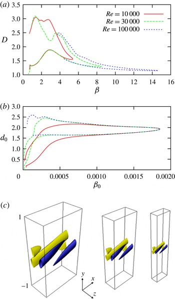
Our starting point is the known steady exact coherent structures of VWI type shown in figure 1(a), where the wavenumber dependence of the drag on the lower wall $D$ is plotted for various $\mathit{Re}$ . This solution is the same as that discussed in Nagata (Reference Nagata1990), Wang et al. (Reference Wang, Gibson and Waleffe2007), Hall & Sherwin (Reference Hall and Sherwin2010), Blackburn, Hall & Sherwin (Reference Blackburn, Hall and Sherwin2013) and Deguchi & Hall (Reference Deguchi and Hall2014a ,Reference Deguchi and Hall b ). The asymptotically converged branches at relatively small ${\it\beta}$ in the figure correspond to VWI. It has been shown by Blackburn et al. (Reference Blackburn, Hall and Sherwin2013) that increasing the wavenumbers causes the VWI states to begin to localize around $y=0$ . Here, we further find that when the wavenumbers become larger and reach a certain threshold size, the convergence of VWI is lost, as the deviation of the saddle-nodes at different $\mathit{Re}$ in the figure suggests. The breakdown of the asymptotic convergence is in fact a signature of new asymptotic structure, which can be seen in the rescaled drag–wavenumber plot shown in figure 1(b), and in the self-similar flow fields at the saddle-nodes shown in figure 1(c). Approximately 200–300 Chebyshev polynomials are used in $y$ to resolve the vertically localized structures. The precise definitions of the scaled wavenumber ${\it\beta}_{0}\approx \mathit{Re}^{-1/2}{\it\beta}$ and the scaled drag $d_{0}\approx \mathit{Re}^{1/2}{\it\beta}_{0}(D-1)$ used in figure 1(b) are to be deduced in our generalized asymptotic analysis below.

First, it is convenient to define a streamwise average operator $\overline{I}(f)=({\it\alpha}/2{\rm\pi})\!\int _{0}^{2{\rm\pi}/{\it\alpha}}f\,\text{d}x$ and $\widetilde{I}(f)=f-\overline{I}(f)$ for a function $f(x,y,z)$ . Using these operators, the total flow can be decomposed into the ‘vortex’ component $[\overline{\boldsymbol{u}},\overline{p}]=\overline{I}([\boldsymbol{u},p])$ and the ‘wave’ component $[\widetilde{\boldsymbol{u}},\widetilde{p}]=\widetilde{I}([\boldsymbol{u},p])$ . For the vortex component we refer to $\overline{u}$ as streak and $[\overline{v},\overline{w}]$ as roll. Then, we apply a scaling

where ${\it\gamma}$ is the wavenumber ratio ${\it\beta}/{\it\alpha}$ , and the parameter $Q$ is to be specified later. The size of the wave amplitude ${\it\rho}$ is also to be fixed so that the wave drives the vortex. The scaling makes the vortex part of (2.1) fully viscous as while the size of the viscous term in the wave part of (2.1) is controlled by the parameter $Q$ as where ${\it\Delta}=\partial _{YY}+\partial _{ZZ}$ . Here we assume steadiness of velocity fields for the sake of simplicity, but clearly the following analysis is applicable to travelling waves if we apply Galilean transformation. Notice that the periodic domain is normalized as $X\in [0,2{\rm\pi}]$ and $Z\in [0,2{\rm\pi}]$ , and that no approximation has been made at this stage. As a consequence of the decomposition, we see that the vortex equations (2.3)–(2.4) must be forced by the Reynolds stress terms appearing on the right-hand side of (2.3). If these terms are not present, the vortex component must ultimately decay due to the absence of the energy input.

Figure 1.

The wavenumber dependence of the steady solutions. The wavenumber ratio is fixed as ${\it\beta}/{\it\alpha}=2$ . (a) The variation of the drag $D$ against the change of ${\it\beta}$ . (b) The same result as (a) but both axes are rescaled. The scaled drag and wavenumber are defined as $d_{0}=({\it\beta}/D)(D-1)\approx \mathit{Re}^{1/2}{\it\beta}_{0}(D-1)$ and ${\it\beta}_{0}=\sqrt{({\it\beta}^{2}-{\it\beta}d_{0})/\mathit{Re}}\approx \mathit{Re}^{-1/2}{\it\beta}$ , respectively. (c) The flow fields at the saddle-nodes. $\mathit{Re}$ increases from left to right. The yellow and blue surfaces represent $\pm 50\,\%$ streamwise vorticity.

When ${\it\beta}\sim O(1)$ , we must apply the no-slip conditions on the walls in the vertical direction. However, if ${\it\beta}$ becomes asymptotically large, the conditions may be changed if we consider the nonlinear interaction is localized in a ‘production layer’ of thickness $O({\it\beta}^{-1})$ where the coherent structure is produced; see figure 1(c). This means that we assume the walls do not affect the state and the problem can be simplified to that of an infinite domain in the $y$ direction with matching conditions to the outer flow. Hereafter, we assume all the scaled variables $[U,V,W,P,X,Y,Z]$ are $O(1)$ in the production layer, and we require that outside the layer the wave components decay for large $|Y|$ , and the vortex components return to the unforced linear shear as

where $d_{0}$ is determined as a part of a solution. Thus, from (2.2c ) and (2.7), above and beneath the production layer, the flow must be in the form

where $+$ and $-$ refer to the solutions above and beneath the production layer, respectively. These solutions of linear profile are valid solutions for whole outer regions. The gradient of the outer flow (2.8) must be equal to the drag $D$ , and $d_{0}={\it\beta}(D-1)/D$ must be satisfied from the boundary conditions on the wall. From these conditions we have

The treatment of the matching to the outer flow is similar to that given in Deguchi & Hall (Reference Deguchi and Hall2014a ).

Figure 2.

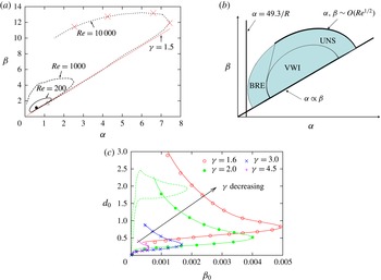
(a) Existence region of the steady solutions in the wavenumber plane. The circle shows $({\it\alpha},{\it\beta})=(0.58,1.15)$ where the solutions first emerge at $\mathit{Re}=127.7$ ; see Clever & Busse (Reference Clever and Busse1997). The triangle is the minimal flow unit $({\it\alpha},{\it\beta})=(1.14,1.667)$ given by Hamilton, Kim & Waleffe (Reference Hamilton, Kim and Waleffe1995). The crosses correspond to the saddle-nodes shown in (c). (b) A schematic picture of the existence region inferred from our generalized asymptotic analysis. (c) Bifurcation diagram of the steady solutions for various ${\it\beta}/{\it\alpha}={\it\gamma}$ . The curves are for $\mathit{Re}=30\,000$ , while the points are for $\mathit{Re}=10\,000$ . The saddle-nodes of asymptotically converged solutions shown by the solid curves define the crosses in (a). The dashed curve shows the branch seen in figure 1(a) for $\mathit{Re}=30\,000$ .

Now, let us consider asymptotically large $\mathit{Re}$ . Three distinct types of asymptotic theories can be considered depending on the size of $Q$ and ${\it\gamma}$ . The first case corresponds to VWI appearing when $Q\gg 1$ ; see Hall & Smith (Reference Hall and Smith1991), Hall & Sherwin (Reference Hall and Sherwin2010), Blackburn et al. (Reference Blackburn, Hall and Sherwin2013) and Deguchi & Hall (Reference Deguchi and Hall2014a ,Reference Deguchi and Hall b ). In this case (2.5) becomes inviscid apart from the critical layer occurring when $\overline{U}$ is small. As shown in Hall & Smith (Reference Hall and Smith1991), outside the critical layer (2.5)–(2.6) can be reduced to Rayleigh’s equation for the streak, which has a singularity at the critical layer and thus produces a large-amplitude neutral wave there. Inside the critical layer of relative thickness $O(Q^{-1/3})$ , the wave Reynolds stress drives the vortex component when ${\it\rho}=\mathit{Re}^{-1}Q^{-1/6}$ . The massive reduction of the equations in the critical layer allows us to handle the structure there almost analytically, as found in Hall & Smith (Reference Hall and Smith1991).

As shown in figure 2(a), the full Navier–Stokes steady solution first appears at $\mathit{Re}=127.7$ and then its existence region expands with increasing $\mathit{Re}$ . In the wavenumber plane, VWI describes the behaviour of the solutions at the centre of the existence region; see the schematic picture in figure 2(b). The states with wavenumbers of $O(1)$ correspond to the edge of laminar–turbulent attractors discussed by Wang et al. (Reference Wang, Gibson and Waleffe2007). In this case, since the basic flow is inviscidly stable from Rayleigh’s inflection point theorem, $\overline{U}$ must have an $O(1)$ deviation from the basic flow to generate a Rayleigh wave. When the wavenumbers are increased, the solutions have a vertically localized structure, which is self-similar for fixed ${\it\gamma}$ , as shown by Blackburn et al. (Reference Blackburn, Hall and Sherwin2013) and Deguchi & Hall (Reference Deguchi and Hall2014a ); the former authors claim that the wave energy of the states satisfies Kolmogorov’s $5/3$ rule. There exists a critical value of ${\it\gamma}\approx 1.5$ at which the solutions cease to exist. This boundary is consistent with the minimal box size to sustain numerical turbulence reported by Hamilton et al. (Reference Hamilton, Kim and Waleffe1995).

The second case occurs when $Q,{\it\gamma}\sim O(1)$ and corresponds to the new structure seen in figure 1. This case is similar to the structure found by Deguchi & Hall (Reference Deguchi and Hall2014c ) for boundary layer flows, where no term drops off from the Navier–Stokes equations at the limit, although here we must consider asymptotically large wavenumbers as we have seen in figure 1. In fact, it is easy to confirm that in the production layer (2.1) can be rescaled into unit Reynolds number Navier–Stokes equations (UNS) by using the velocity scale $[u]\sim \mathit{Re}^{-1/2}$ and the length scale $[x]\sim \mathit{Re}^{-1/2}$ for all three components. The scaling can be found from (2.2a )–(2.2c ) together with the fact that ${\it\rho}$ must be $O(\mathit{Re}^{-1})$ to drive the vortex, or alternatively from the viscous–convective balance $[u][x]\sim \mathit{Re}^{-1}$ and $[u]\sim [x]$ from (2.7). The wavenumber must be expanded as ${\it\beta}={\it\beta}_{0}\mathit{Re}^{1/2}+\cdots \,$ and this means that it is appropriate to define ${\it\beta}_{0}=1/\sqrt{{\it\gamma}Q}$ so that ${\it\beta}$ satisfies

using (2.9). From (2.9)–(2.10), $d_{0}$ and ${\it\beta}_{0}$ can be computed from $D$ , ${\it\beta}$ and $\mathit{Re}$ to confirm the asymptotic convergence of UNS states as seen in figure 1(b). The fact that no reduction is possible in the production layer implies that the analysis there must rely on computations as opposed to the semi-analytic critical layer analysis. In fact, production layer solutions are most easily obtained by applying the knowledge of the asymptotic theory to the Navier–Stokes computations for high Reynolds number. In the wavenumber plane, UNS states describe the large-wavenumber boundary of the existence region as shown in figure 2(b). The crosses indicated at the numerically obtained boundary in figure 2(a) correspond to the asymptotically converged saddle-nodes shown by solid curves in figure 2(c). In the continuation process of the solution branch in the parameter space, it is found that the branch behaves in a complicated way and several families of saddle-nodes appear. The family of saddle-nodes corresponding to the solid curve in figure 2(c) is found to be different from that seen in figure 1 (the same result is shown by a dashed curve in figure 2 c). We can connect these solution branches by changing wavenumbers.

In the third case, $Q\sim O(1)$ and ${\it\gamma}\gg 1$ , and (2.1) reduces to boundary region equations (BRE), i.e. the streamwise derivative is neglected in the pressure and viscous terms in the Navier–Stokes equations; see Deguchi et al. (Reference Deguchi, Hall and Walton2013). We can prove that there is no BRE-type solution for streamwise wavenumber smaller than some particular threshold. As shown in Deguchi et al. (Reference Deguchi, Hall and Walton2013), that threshold is given by ${\it\alpha}=49.3/\mathit{Re}$ for plane Couette flow; see figure 2(a). However, notice that numerical evidence has shown that some solutions developing multiple spatial scales in $x$ could exist beyond that threshold because it is only applicable for purely BRE-type solutions; see Avila et al. (Reference Avila, Mellibovsky, Roland and Hof2013), Brand & Gibson (Reference Brand and Gibson2014), Deguchi & Hall (Reference Deguchi and Hall2014b ) and Zammert & Eckhardt (Reference Zammert and Eckhardt2014) for numerical evidence of the multiple-scale solutions. The longest streamwise wavelength structure, where the BRE-type problem predicts ${\it\alpha}\sim O(\mathit{Re}^{-1})$ , carries a largest $O(1)$ disturbance, and thus may be related to the energetic very large-scale motion observed in Morrison et al. (Reference Morrison, McKeon, Jiang and Smits2004).

3. Discussion and conclusions

Importantly, the UNS-type exact coherent structures found in this study are fully viscous and thus must have a Kolmogorov length/velocity scale. 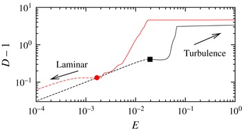In fact, by using a dimensional energy dissipation rate ${\it\Phi}={\it\nu}(U_{\ast }/h_{\ast })^{2}$ , we can find the Kolmogorov length scale ${\sim}({\it\nu}^{3}/{\it\Phi})^{1/4}=\mathit{Re}^{-1/2}h_{\ast }$ and Kolmogorov velocity scale ${\sim}({\it\nu}{\it\Phi})^{1/4}=\mathit{Re}^{-1/2}U_{\ast }$ consistent with the discussion in the last section. Although the solutions of this type have a very small disturbance size, some of them can trigger a transition to turbulence. Figure 3 shows the typical direct numerical simulations starting from the UNS- and VWI-type solutions perturbed by a small random disturbance. Both solutions sit at the laminar–turbulent boundaries, but UNS-type solutions have much smaller disturbance kinetic energy $E$ , averaged in the periodic box. Note that, in an asymptotic sense, any disturbance of smaller size must dissipate since only the viscous terms play a major role. Therefore UNS states represent the theoretically minimal self-sustained states. Another implication of our theory is that no reduced model can be considered for such minimal-scale coherent structures, since we need to keep all terms in the Navier–Stokes equations.

Figure 3.

The direct numerical simulation for $\mathit{Re}=10\,000$ . A periodic box $(x,y,z)\in [0,2{\rm\pi}/1.5]\times [-1,1]\times [0,2{\rm\pi}/3]$ is resolved by $145\times 410\times 98$ grid points. The circle is the UNS-type solution for $({\it\alpha},{\it\beta})=(6,12)$ ; this solution is close to the saddle-node of the solid curve for ${\it\gamma}=2$ in figure 2(c). The square is the VWI-type solution for $({\it\alpha},{\it\beta})=(1.5,3)$ at the lower branch of figure 1(a). The solutions are perturbed by random disturbances with $E\sim O(10^{-16})$ , and the two typical results are shown for each solution. Note that for the laminar flow $(D,E)=(1,0)$ . The turbulent trajectory is not shown since the resolution used is insufficient to produce correct turbulent statistics.

In view of much numerical evidence for the existence of the multiple-scale solutions localized in $(x,z)$ , for example Brand & Gibson (Reference Brand and Gibson2014) and Zammert & Eckhardt (Reference Zammert and Eckhardt2014), a localized version of our minimal scale states may also exist. It is noteworthy that such localized minimal states would have an energy scaling $E\sim \mathit{Re}^{-2.5}$ in a fixed periodic box, which is close to that obtained by an energy-optimized technique, $E\sim \mathit{Re}^{-2.7}$ ; in fact, the optimized states typically have localized structures as seen in Duguet et al. (Reference Duguet, Monokrousos, Brandt and Henningson2013).

Although our focus so far has been on steady solutions, the scenario elucidated here can be applicable for any form of UNS solutions, such as travelling-wave, time-periodic or even chaotic solutions, by introducing a time scale ${\sim}[x]/[u]$ . Furthermore, similar to the localized VWI proposed by Blackburn et al. (Reference Blackburn, Hall and Sherwin2013), the UNS results found in plane Couette flow can be embedded for any background flow as long as the flow can be locally approximated by a linear shear in the asymptotic sense. When that local approximation is not applicable, we need to consider different far-field boundary conditions for UNS. For example, at a point where the background shear vanishes, a local approximation of the background flow may be proportional to the square of the vertical coordinate after an appropriate Galilean transformation. Thus the far-field condition (2.7) must be replaced by $\overline{U}\rightarrow Y^{2}$ to leading order. Such a UNS problem can be solved at the centre of the plane Poiseuille flow, where the basic flow takes the form of $\boldsymbol{u}=[1-y^{2},0,0]$ . 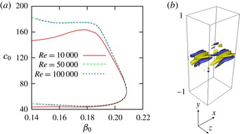Figure 4 shows an example of such UNS-type solutions. Notice that in general the UNS states must travel with a local basic flow speed plus a correction of order $[u]$ . The appropriate wavenumber scaling ${\sim}[x]^{-1}$ can easily be found by considering the viscous–convective balance $[u][x]\sim \mathit{Re}^{-1}$ and the far-field condition $[u]\sim [x]^{2}$ . The scaling $[u]\sim \mathit{Re}^{-2/3}$ , $[x]\sim \mathit{Re}^{-1/3}$ can be confirmed in figure 4(a), where the scaled wave speed and wavenumber are plotted. Likewise at the edge of boundary layers, the form of the background flow is typically of exponential function form, and in fact this case corresponds to the free-stream coherent structures observed at the edge of boundary layers; see Deguchi & Hall (Reference Deguchi and Hall2014c ). However, notice that the states discussed here are completely trapped in the production layer whilst the free-stream coherent structures generate a large streak beneath the production layer.

Figure 4.

(a) The bifurcation diagram of the plane Poiseuille flow solutions for ${\it\gamma}=4/3$ . The solutions are obtained from TW1-1 found in Gibson & Brand (Reference Gibson and Brand2014) and thus are of the travelling-wave form propagating in $x$ with a phase speed $c$ . To show the solutions are of UNS type, $c_{0}=(1-c)Re^{2/3}$ and ${\it\beta}_{0}=\mathit{Re}^{-1/3}{\it\beta}$ are used in the diagram. (b) The flow field at the saddle-node for $\mathit{Re}=100\,000$ . See the caption to figure 1 for the definition of the surfaces.

The UNS-type structures may also be found in the near-wall region of turbulent shear flows, where small-scale coherent structures play a major role. When the UNS structure is close to the wall we must apply no-slip conditions at finite $Y$ instead of one of the far-field conditions. The near-wall fine-scale exact coherent structures found by Gibson & Brand (Reference Gibson and Brand2014) are likely to have a UNS limit of this kind.

In conclusion, we have found an asymptotic theory for large Reynolds number that describes self-sustained nonlinear coherent structures at Kolmogorov microscale. The self-sustaining mechanism of the structure is governed by unit Reynolds number Navier–Stokes equations in an unbounded domain. Solutions of that canonical problem can be found by directly solving simple parallel flows at large Reynolds number. The asymptotic solutions obtained in this way define the theoretically minimal-scale self-sustained structures that can be embedded at a local position of almost arbitrary shear flows. Our numerical computation suggests that some disturbances at Kolmogorov scale can initiate a turbulent transition despite their finite but asymptotically small size. Therefore, our results seems to be an important stepping stone to elucidating the puzzling property of shear flows noticed by Sommerfeld (Reference Sommerfeld1908). Notice that the conclusion drawn here does not contradict the belief that some numerically obtained optimal disturbances are on the stable manifold of the edge state of VWI/self-sustaining process type, as the UNS-type equilibrium states could have a heteroclinic connection to the edge state.