

Introduction
Large amounts and types of data are continuously made available by different proximal and remote sensors with their particular sensing modes. Therefore, it is common that different instruments are used in conjunction with one another (data fusion) to take advantage of their complementary characteristics. Data fusion is defined as “the process of combining information from heterogeneous sources into a single composite picture of the relevant process, such that the composite picture is generally more accurate and complete than that derived from any single source alone” (Hall & McMullen, Reference Hall and McMullen2004). However, there is not yet a single, well established data fusion methodology for combining sensor data in a rigorous way. Moreover, depending on context, ‘data fusion’ may assume different meanings such as information fusion, sensor fusion or image fusion. Information fusion is the process of merging information from different sources; sensor fusion is the combination of data from different sensors and image fusion is the fusion of two or more images into one, which should be a more useful image. Furthermore, the data may have different spatial resolutions (support sizes), shapes and configurations, and their combination results in the problem of change of support. Failure to address such a problem might result in erroneous conclusions when inferences drawn from aggregated data are applied to point units (Nguyen et al., Reference Nguyen, Katzfuss, Cressie and Braverman2014). To merge such data, ad hoc methods are often used in many GIS packages. Union, intersection, zonal averaging, pixel-by-pixel computations between two rasters with different supports are some of the fusion operations feasible in GIS software. These methods have the advantage of being fast and scalable, but they do not treat the change of support problem. Consequently, there is ambiguity about the support of the output and there is no measure of uncertainty associated with the input or the prediction (Nguyen et al., Reference Nguyen, Katzfuss, Cressie and Braverman2014).
A data fusion approach from a statistical point of view aims to combine heterogeneous samples statistically from marginal distributions to make inferences about the unobserved joint distributions or functions of them (Braverman, Reference Braverman2008). Although this approach treats the problem of change of support and the assessment of uncertainty explicitly, it is not directly applicable to spatial datasets because it assumes that observations are independent of one another, which is generally not true for spatial data. Various methodologies have been developed to account for covariance in spatial datasets; geostatistics is a branch of applied statistics that deals specifically with spatial relations. Geostatistics enables rigorous treatment of spatial correlation by using a mathematical model, called variogram, and a class of methodologies, called kriging, which calculate the mean-squared prediction errors.
Lajaunie (Reference Lajaunie1996) developed a methodology, called mixed support kriging (MSK), based on the theory of random kriging (Journel & Huijbregts, Reference Journel and Huijbregts1978), which aims to solve a kriging system when the data are on different supports. The MSK has been used in the analysis of mineral resources by Bush (Reference Bush2010) to optimize the prediction of diamond concentrations from all available data on different sizes of support.
The objective of this paper is to propose a methodology within a geostatistical framework to solve the issues of heterogeneous spatial support for estimation in a spatial context. In this paper, MSK was applied to the outcomes of a multiple frequency sensor to produce a map of apparent electrical conductivity for the soil of an agricultural field, which could be used for field partition in the scope of site-specific management.
Materials and methods
Study area
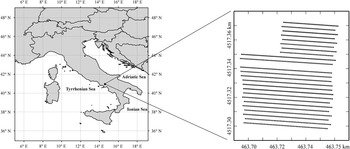
The study area (Figure 1) is located in the Campania region (central Italy) on the plain of the Sarno river and is characterised by an alluvial system that produces stony-sandy soils in silt matrix. The climate is Mediterranean with winter characterised as rather mild and rainy, whereas the summer is very hot and dry (Longobardi et al., Reference Longobardi, Buttafuoco, Caloiero and Coscarelli2016).
Study area and sample data locations.

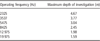
In 2014, a soil survey was carried out to measure the apparent soil electrical conductivity (ECa, mS m−1) in a field (0.4 ha) cropped with San Marzano tomato. The ECa was measured by a multiple frequency electromagnetic profiler GEM300® (Geophysical survey Systems, Inc. USA), which was set at six operating frequencies (19 975; 12 975; 8425; 5475; 3575 and 2325 Hz) with the coils in a vertical orientation. Each operating frequency had a different depth of investigation and therefore explored a different soil volume. The maximum depth of investigation (Table 1) was calculated as the square root of skin depth (Daniels et al., Reference Daniels, Vendl, Ehsani and Allred2008), choosing a detection threshold of 30% for soil conductivity less than 50 mS m−1 (Huang, 2005; Reynolds, Reference Reynolds2011). The survey was carried out along 24 transects (Figure 1).
Maximum depth of investigation associated with each operating frequency

Data analysis: Geostatistical and statistical procedures
Random kriging (RK) (Maréchal and Serra, Reference Marechal and Serra1970; Journel & Huijbregts, Reference Journel and Huijbregts1978) is based on a simplified version of block kriging, which estimates a value over a block V (support) as a weighted average of the data values on a point support at the locations X i :
 $$Z^{{\asterisk}} (V)\,{\equals}\,\mathop{\sum}\limits_i^{} {\lambda _{i} Z({\bf X}_{i} )}. $$
The particular feature of RK is that the point value Z at X i is replaced by a block estimate over a block V that contains the point X i , but it is assumed to be located at a random point x i within the same block V. This is an interesting way to homogenize the data to the same support so that punctual kriging (Webster and Oliver, Reference Webster and Oliver2007) can be applied. If it is assumed that the position of the datum point is random within the block and independent of the positions of the other data points, the covariance between two data points is given by:
 $${\rm Cov}\left\{ {Z(v_{i} ),Z(v_{j} )} \right\}\,{\equals}\,\overline{C} (V_{i} ,V_{j} ){\equals}{1 \over {V_{i} }}{\times}{1 \over {V_{j} }}\mathop{\int}\limits_{V_{i} } {} \mathop{\int}\limits_{V_{j} } {C(x{\minus}y)dxdy} ,$$
where
 $$C(x{\minus}y)$$
refers to the covariance model on a point support, v
i
and v
j
refer to the volumes of two distinct supports and
 $$\overline{C} (V_{i} ,V_{j} )$$
is the block covariance. This means that the point–point covariance can be calculated as the block covariance for the distance between the two centroids of the blocks that contain the data. Equation (2) remains valid even when i and j represent two different data points within the same block, and then the two supports are the same. Therefore, the diagonal terms of the kriging system depend only on the different supports v
i
and their dispersion variances within the domain D of study,
 $$\sigma _{{v_{i} }}^{2} $$
.
Random kriging or mixed support kriging (MSK) is quite similar to classical kriging with the difference that each datum has its own variance, which amounts to performing kriging with the variance of the measurement error (Chilès and Delfiner, Reference Chilès and Delfiner2012). In MSK, the diagonal of the kriging system is modified by adding a variance specific to each datum, which generally stems from uncertainty associated with the measurement. In the case of MSK, the variance represents the dispersion variance of the data support, v
i
, in the estimation block V (
 $${\rm var}\left( {v_{i} \left| V \right.} \right)$$
).
When the variogram model is estimated over the block support, the diagonal term in the kriging system is the sum of two components: the dispersion variance of blocks within the domain (
 $$Var\left( {V\left| D \right.} \right)$$
) and dispersion variance of the support within the block (
 $$Var\left( {v{}_{i}\left| V \right.} \right)$$
). Therefore, in accordance with the variance additivity relation, the dispersion variance of the support within the domain is given by:
 $${\rm var}\left( {v{}_{i}\left| D \right.} \right)\,{\equals}\,{\mathop{\rm var}} \left( {v{}_{i}\left| V \right.} \right){\plus}\left( {V\left| D \right.} \right)\,{\equals}\,\sigma _{{v_{i} }}^{2} $$
as required by MSK.
In summary, MSK is performed in two steps:
-
∙ Calculation of the dispersion variance of the support within the block to be kriged, i.e. (
 $$Var\left( {v_{i} \left| V \right.} \right)$$
), with the parameters from the point variogram model;
-
∙ Block kriging with parameters of the block variogram model, and with the variance of the measurement error calculated in the previous step.

To model variogram on a point support, the variogram was calculated on the smallest support, corresponding to the highest operating frequency (19 975 Hz). All other supports were considered as multiples of the point support on the basis of the effective soil depth surveyed by the lower frequencies. The point variogram was then regularised over each parallelepiped (support), whose dimensions were determined previously. The data were interpolated over blocks of 2 m by 2 m by 1.5 m. Each map for the different operating frequencies represents a different picture of the same object and their differences stem mostly from the different volumes of soil crossed by the electromagnetic waves with different frequencies. More exhaustive information can be obtained through a proper combination of all these maps, which take into account the different amounts of uncertainty. To do that and with the objective to delineate homogeneous zones within the field for site specific management, a direct and fast approach is the weighted principal component analysis (WPCA) where the weight function is given by the dispersion variance.
The mixed support kriging was implemented in ISATIS® software (Geovariances, 2016).
Results and Discussion
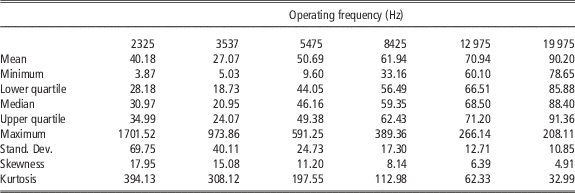
Six channels of soil bulk electrical conductivity (ECa) data were available corresponding to the different frequencies and different soil volumes (supports) that they were associated with (Table 1). Given the particular arrangement of the measurement equipment, all the data types have the same number of observations at the same locations on the soil surface. The summary statistics of ECa data at the different frequencies showed a considerable departure from a normal distribution (Table 2). Therefore, all data were normalized by fitting a multivariate Gaussian anamorphosis mathematical model (Wackernagel, Reference Wackernagel2003; Castrignanò and Buttafuoco, Reference Castrignanò and Buttafuoco2004).
Basic statistics of ECa (mS m−1) data at the different operating frequencies

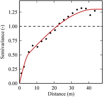
To implement MSK, the first step was to create a new file for storing the samples, which were moved to the centres of the blocks (V) of the interpolation grid and to calculate the dispersion variance of the data support within the block. A punctual variogram model, based on the smallest support associated with the frequency of 19 975 Hz, was fitted including a nugget effect and two spherical models with ranges of 6.39 m and 40.21 m (Figure 2), i.e. a nested spherical function.
Experimental and model punctual variogram for Gaussian ECa (−) data at the operating frequency of 19 975 Hz.

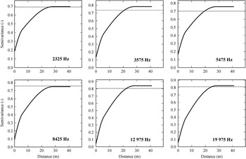
The variograms for a block support were obtained by regularization over the supports; they are shown in Figure 3.
Regularised variograms of Gaussian ECa (−) data at the different operating frequencies.

The nugget effect for all supports was calculated by the ratios of the ‘punctual’ support volume and of the other support volumes. The same type of mathematical model was fitted to all block variograms, including a nugget effect and two spherical models with ranges of 5.7 m and 28.27 m. As it can be seen from the Figure 3, there is a tendency for the sills of the variograms to decrease as a function of the reduction in frequency and of the increase in size of support. This effect can be explained by integration of the electromagnetic signal over a larger volume of soil.
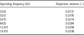
The assessment of the dispersion variance (Table 3), corresponding to the different frequencies, confirmed the previous result, i.e. that the variance varied as a direct function of frequency, due to the bigger soil volume explored by lower frequencies.
Dispersion variance of Gaussian ECa data associated with each operating frequency

The ECa responses associated with the higher frequencies are noisier, but they have a finer spatial resolution. This result highlights the need to account for the different statistical properties of each signal, which also means that their different degrees of uncertainty must also be taken into account when jointly analysing the outcomes of different sensors. Each sensor produces a different image with a different degree of reliability of the same object. Precision and spatial resolution are often conflicting characteristics of the same sensor and they need to be assessed accurately to make the optimal choice of the sensors for the study of the processes of primary interest.
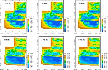
Figure 4 shows the ECa maps obtained with MSK at the selected operating frequencies.
Maps of ECa (mS m−1) at the selected frequencies.

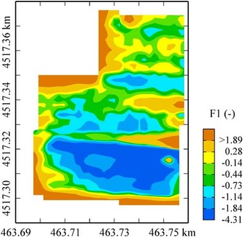
The maps for the different operating frequencies look quite similar, but they do differ in their absolute values and corresponding error variances. To aggregate and summarise these maps, the first principal component of the weighted principal component analysis (WPCA), as a new variable, was used for the management zones delineation. The first principal component explains more than 91% of the total variance and the resultant map is shown in Figure 5.
Map of the first component from the weighted principal component analysis (WPCA).

The map (Figure 5) reproduces the main spatial structures observed in each individual map, but it combines them. It enhances the contribution of the shallow soil, and so gives an integrated representation of the whole soil profile which was effectively explored by the electromagnetic waves.
The N–S field partition was associated with the differences in soil texture and in the variable depth of the shallow groundwater, which affects local soil water content (internal report not published). This information is valuable for planning site-specific irrigation
Conclusions
The question of the best way to integrate different types of data to derive the most information is a common problem. At present environmental databases often include the outcomes from different sensors, characterised by various spatial resolutions and degrees of uncertainty. From a statistical point of view, disregarding the heterogeneity of data, by merging all data together, might lead to considerable estimation errors and bias. Geostatistics can produce a satisfactory solution to this common problem by taking the change of support into account. Mixed support kriging, which is essentially the method of kriging with variance of the measurement error, can provide unbiased estimates and improve the precision of estimation. Moreover, the increase in use of GIS systems makes the problem of change of support a crucial issue. Valid methods for combining different spatial data might be implemented in GIS systems in the near future to ensure that proper methods are used for spatial analysis.
Acknolowledgements
Financial support for this work comes from the project “M2Q” PON03PE_00180_1 co-funded by the National Operational Programme for Research and Competitiveness (PON R&C) 2007–2013, through the European Regional Development Fund (ERDF) and national resource (Revolving Fund – Cohesion Action Plan MIUR). D.M. MIUR n. 738/05.03.2014.
The authors thank Dr. Margaret A. Oliver and an anonymous reviewer for providing constructive comments, which have contributed to the improvement of the published version.