1. Introduction
Precise pose estimation is one of the key technologies for mobile robots. It is a prerequisite for performing some useful tasks, such as workshop docking [Reference Yilmaz and Temeltas1] and indoor cleaning. Catastrophic consequences may follow with false pose estimation. Robot localization techniques can be roughly divided into two classes [Reference Borenstein, Everett and Feng2]: pose tracking and global localization. They can be distinguished by the state space in which they operate [Reference Burgard, Derr, Fox and Cremers3]. Pose tracking assumes that the initial robot pose is known and solely explores a small state space generally centered around the estimated pose since the uncertainty is local. Global localization assumes that the initial robot pose is unknown, and needs to deal with the complete state space because of global uncertainty.
Wheel encoders and LiDAR are two commonly used sensors for indoor mobile robots. A mobile robot equipped with wheel encoders can compute an estimate of its pose (odometry) by dead reckoning that has advantages in local consistency and smoothness. However, the trajectory will drift due to error accumulation [Reference Peng and Weikersdorfer4]. Actually, the task of pose tracking is the correction of accumulated dead reckoning errors caused by the inherent inaccuracy of wheel encoders and other factors such as slipping [Reference Burgard, Fox and Hennig5]. LiDAR can provide accurate distances to obstacles and is not sensitive to illumination. Correlating LiDAR scan with prior map can correct accumulated odometry errors effectively making LiDAR popular in robot localization.
Scan matching is the process of translating and rotating a range scan in such a way that a maximum overlap between sensor readings and a priori map emerges [Reference Gutmann, Burgard, Fox and Konolige6]. Both ICP [Reference Besl and McKay7]–[Reference Serafin and Grisetti11] and NDT [Reference Biber and Strasser12, Reference Magnusson, Lilienthal and Duckett13] depend on initial guess to provide a reliable result and therefore are not suitable to address global localization problem. Correlative scan matching (CSM) [Reference Olson14] finds rigid-body transformation that maximizes the probability of having observed data. It performs a search over the entire space of plausible candidates making it robust to initial error and capable of addressing both pose tracking and global localization problems. CSM has benefited some famous SLAM systems [Reference Konolige, Grisetti, Kümmerle, Burgard, Limketkai and Vincent15, Reference Hess, Kohler, Rapp and Andor16].
Monte Carlo Localization (MCL) [Reference Dellaert, Fox, Burgard and Thrun17, Reference Fox, Burgard, Dellaert and Thrun18] is a very popular localization approach in the robotics research community and has been shown to be robust in many practical applications [Reference Röwekämper, Sprunk, Tipaldi, Stachniss, Pfaff and Burgard19, Reference Vasiljević, Miklić, Draganjac, Kovačić and Lista20]. However, its localization precision is somewhat low. The repeated experiment in ref. [Reference Röwekämper, Sprunk, Tipaldi, Stachniss, Pfaff and Burgard19] shows that average localization error of MCL is 6 cm at a grid resolution of 5 cm. In addition, MCL needs the robot to move continually during global localization, which may take a long time to recover from localization failures. Jari Saarinen et al. [Reference Saarinen, Andreasson, Stoyanov and Lilienthal21] proposed Normal Distributions Transform Monte Carlo Localization (NDT-MCL), whose best mean accuracy is 2.4 cm in the dynamic test and is lower than 2 cm in the both static and slip test. But this approach requires the Normal Distributions Transform Occupancy Map (NDT-OM) proposed in ref. [Reference Saarinen, Andreasson, Stoyanov, Ala-Luhtala and Lilienthal22] and does not consider global localization problem. Naoki Akai [Reference Akai23] presented a reliable MCL method that is composed of pose tracking and global localization. However, there is a tradeoff relationship between robustness and accuracy in its pose tracking and the global localization module may not always stably work.
In this paper, we develop a more capable localization method achieving precise pose tracking as well as quick global localization using CSM. In pose tracking problem, the accumulated odometry errors are corrected by CSM within a small search space centered around the predictive pose. A low-pass filter associating predictive pose with corrected pose is applied to improve precision and smoothness. In global localization problem, the global pose is retrieved by CSM within the complete search space. The branch-and-bound method is employed to minimize the volume of evaluated candidates and substantially improve search efficiency. We have validated the proposed method in simulated, public datasets-based and real environments. The main contributions of this paper are summarized as follows:
-
• Construct a localization system integrating a precise pose tracking module with a fast global localization module based on CSM, which will benefit the indoor mobile robots equipped with 2D-LiDAR.
-
• Import a compact low-pass filter utilizing covariance estimates obtained from CSM to improve precision and smoothness of the pose tracking module.
-
• Utilize branch-and-bound method to accelerate the global localization module.
-
• Design several trigger criteria to detect localization failures in time.
The rest of this paper is organized as follows: Section 2 reviews related work about mobile robot localization based on LiDAR. Section 3 gives an overview of our method. Sections 4 and 5 describe pose tracking module and global localization module respectively in detail. Section 6 presents experiments and results. Section 7 finally concludes the paper.
2. Related work
Self-localization is a fundamental prerequisite for mobile robots that has received significant attention in the past thirty years [Reference Yekkehfallah, Yang, Cai, Li and Wang24, Reference Ma, Jiang, Ou and Xu25]. In this section, we solely concentrate on the LiDAR-based localization methods and will review related work from the point of sensor fusion method.
EKF-based localization methods are classical and have been applied to many robot systems [Reference Gutmann, Weigel and Nebel26]–[Reference Zhang, Wang, Jiang, Zeng and Dai29] successfully. The advantage of EKF lies in its high efficiency, while the linearization in its prediction stage will lose certain accuracy. The only one pose hypothesis makes EKF unable to globally localize the robot or recover from localization failures. Furthermore, EKF-based localization is primarily applied to feature-based maps [Reference Thrun, Burgard and Fox30].
Markov localization (ML) can overcome these problems of EKF, whose key idea is to compute and update a probability distribution over all possible locations in the environment [Reference Burgard, Derr, Fox and Cremers3]. Dieter Fox et al. [Reference Fox, Burgard, Thrun and Cremers31] extended ML by an approach that filters sensor data, so that the damaging effect of corrupted data is reduced. Their approach can localize robots under global uncertainty and in highly dynamic environments whose disadvantage, however, is the huge state space that has to be maintained. Wolfram Burgard et al. [Reference Burgard, Derr, Fox and Cremers3] presented Dynamic Markov Localization which dynamically adapts the size of the state space according to the robot’s certainty in its position. It is able to globally localize the robot whenever necessary and efficiently keep track of the robot’s position in normal situations. Kurt Konolige et al. [Reference Konolige and Chou32] introduced a correlation-based ML (CBML) which does not require ray-tracing operations and precomputing with prior map, thereby reducing computational and storage requirements and making it several orders of magnitude more efficient than ML. Andrea Censi [Reference Censi33] developed CBML-O, a variant of CBML, taking into account the orientation information in both scan and map to respect orientation constraints.
MCL is another famous method possessing the ability to cope with both pose tracking and global localization problems. It employs a weighted set of robot pose estimates, termed as particles, to describe the probability distribution. Jens-Steffen Gutmann et al. [Reference Gutmann and Fox34] presented adaptive MCL (AMCL), which tracks short-term and long-term average of the likelihood to control the injection of random particles, thereby adding an additional level of robustness. Dieter Fox [Reference Fox35] introduced KLD-sampling whose key idea is to determine the number of particles based on a statistical bound on the sample-based approximation quality. This scheme increases the efficiency of particle filters by adapting the size of sample sets during the estimation process. Ryuichi UEDA et al. [Reference Ueda, Arai, Sakamoto, Kikuchi and Kamiya36] presented MCL with expansion resetting (EMCL) in which KLD-sampling and adaptive MCL are not implemented. Instead, a blending of expansion resetting and sensor resetting is integrated to allocate particles efficiently. Jose-Luis Blanco et al. [Reference Blanco, Gonzalez and Fernandez-Madrigal37] described optimal filtering algorithm which can dynamically generate the minimum number of particles that best represent the true distribution within a given bounded error, making the method focus on the samples in the relevant areas of the state space better than previous particle filter algorithms. The NDT-MCL method proposed in ref. [Reference Saarinen, Andreasson, Stoyanov and Lilienthal21] formulates the MCL localization approach using NDT as an underlying representation for both map and sensor data. The experiments show that it achieves higher accuracy and repeatability than grid-based MCL. Qi Liu et al. [Reference Liu, Di and Xu38] proposed 3DCF-MCL combining the high accuracy of the 3D feature points registration and the robustness of particle filter, which can provide accurate and robust localization for autonomous vehicles with 3D point cloud map. Naoki Akai [Reference Akai23] presented a reliable MCL method which can simultaneously perform robust localization, reliability estimation, and quick relocalization.
Besides the filter-based approaches mentioned above, optimization-based localization methods have been progressively introduced. Mariano Jaimez et al. [Reference Jaimez, Monroy and Gonzalez-Jimenez39] presented range flow-based 2D odometry (RF2O) which expresses the sensor motion estimation as an optimization problem about scanned points by means of establishing the range flow constraint equation [Reference Gonzalez and Gutierrez40]. They extended RF2O in ref. [Reference Jaimez, Monroy, Lopez-Antequera and Gonzalez-Jimenez41] as symmetric range flow-based odometry (SRF-Odometry) that requires the gradients of both scans but has a smaller linearization error. Wendong Ding et al. [Reference Ding, Hou, Gao, Wan and Song42] proposed a loosely coupled localization method integrating a LiDAR inertial odometry together with their matching-based global LiDAR localization module. Both measurements from the two modules are jointly fused in a pose graph optimization framework. Steve Macenski et al. [Reference Macenski and Jambrecic43] presented Slam_toolbox including an optimization-based localization mode. It takes existing map pose graphs and localizes within them with a rolling window of recent scans by quickly adding and removing nodes and constraints from the pose graph. Ruyi Li et al. [Reference Li, Zhang, Zhang, Yuan, Liu and Wu44] designed a tightly coupled laser-inertial odometry and mapping with bundle adjustment (BA-LIOM) to optimize the LiDAR point clouds and keyframe poses as well as the IMU bias in real time. Their approach can considerably decrease the drift of odometry and relieve the issue of ground warping caused by sparse laser scans. Koki Aoki et al. [Reference Aoki, Koide, Oishi, Yokozuka, Banno and Meguro45] presented a 3D global localization method using branch-and-bound algorithm (3D-BBS) that enabled accurate and fast global localization with only a 3D LiDAR scan roughly aligned in the gravity direction and a 3D pre-built map.
Deep learning has been extensively introduced into the robotics community, and learning-based localization attracts significant research interest. Giseop Kim et al. [Reference Kim, Park and Kim46] presented a robust long-term localization method, formulating the place recognition problem as place classification with a convolutional neural network (CNN) and achieving a robust year-round localization performance even when learned in just a single day. Sebastian Ratz et al. [Reference Ratz, Dymczyk, Siegwart and Dubé47] introduced a global localization algorithm relying on learning-based descriptors of point cloud segments. Their approach, which does not require the robot to move, can compute the full 6 degree-of-freedom pose in a map using only a single 3D LiDAR scan at a time. Naoki Akai et al. [Reference Akai, Hirayama and Murase48] proposed a hybrid localization method that fuses MCL and CNN-based end-to-end (E2E) localization. The proposed method utilizing a CNN to sample particles and fusing them with MCL via importance sampling (IS), can smoothly estimate the robot pose, similar to the model-based method, and quickly re-localize it from the failures, similar to the learning-based method. Junyi Ma et al. [Reference Ma, Zhang, Xu, Ai, Gu and Chen49] showcased a lightweight network with the Transformer attention mechanism exploiting the range image representation of LiDAR scans to generate yaw-angle-invariant descriptors. Their approach achieves fast execution with less than 2 ms per frame and at the same time yields very good recognition results in different challenging environments.
3. System overview
Theoretical basis of our method is Bayesian filtering. To find the posterior distribution p( x t | x t-1, u t , z t , m ) over the robot’s state x t , we can obtain Eq. (1) with Bayes’ rule:
 \begin{align}\textit{p}(\boldsymbol{x}_{\textit{t}}\,| \, \boldsymbol{x}_{t-1},\boldsymbol{u}_{t},\boldsymbol{z}_{t},\boldsymbol{m})\propto \textit{p}(\boldsymbol{z}_{t} \,| \,\boldsymbol{x}_{\textit{t}},\boldsymbol{m})\textit{p}(\boldsymbol{x}_{\textit{t}}\, |\, \boldsymbol{x}_{t-1},\boldsymbol{u}_{t})\end{align}
where p( z t | x t , m ) is measurement model characterizing how measurement z t is governed by state x t and environment model m . p( x t | x t-1, u t ) is motion model characterizing how state x t changes with control u t over time. They correspond to the two basic steps of Bayesian filtering for state estimation: predicting the next state based on robot motion, and updating the predicated state based on sensor readings.
Figure 1 depicts the block diagram of our localization method composed of a pose tracking module and a global localization module. In pose tracking module, synchronized odometry
O
m
will be computed firstly by linear interpolation of the raw odometry
O
r
in the light of the time stamp of raw LiDAR scan
S
r
. Outliers of
S
r
will be removed according to the distances from LiDAR points to obstacles in prior map to obtain the outliers-free LiDAR scan
S
m
to be used in CSM. We set fixed translational and angular thresholds for odometry increment
 $\Delta\boldsymbol{O}$
to trigger CSM, namely accumulated odometry errors will be corrected whenever the robot translates a certain distance or rotates a certain angle. A low-pass filter associating the predictive pose
T
p
with the corrected pose
T
c
from CSM is applied to generate the filtered pose
T
l
which is integrated into the final output pose
T
o
. And
T
l
will take part in the next pose prediction. Localization failures will be autonomously detected with our designed trigger criteria and global localization module will recover correct global pose
T
g
quickly when a localization failure occurs.
Block diagram of our localization method. The dotted arrow indicates that global localization is only triggered when necessary.

4. Pose Tracking
Pose tracking assumes that the initial robot pose is known and only requires a small search space due to the local uncertainty. In this section, we will offer a short overview of CSM at first, and then present its practical implementation in detail. Finally, a low-pass filter will be introduced to improve precision and smoothness of the pose tracking module.
4.1. CSM overview
The pose tracking module employs CSM as the scan matcher, which performs a search over the entire space C of plausible rigid-body transformations to find global maximum x m maximizing the probability of having observed the data, namely
 \begin{align}\boldsymbol{x}_{m}= \underset{\boldsymbol{x}_{\textit{i}}\in \textit{C}}{\text{argmax }}\textit{p}(\boldsymbol{z}_{t}\,| \, \boldsymbol{x}_{i},\boldsymbol{m})\end{align}
To compute probability for every single candidate x i efficiently, the assumption of mutual independence for each individual LiDAR return z t,j is applied. So p( z t | x i , m ) can be expressed as:
 \begin{align} p(\boldsymbol{z}_{t}\, |\, \boldsymbol{x}_{i}, \boldsymbol{m} ) = \prod\nolimits _{\textit{j}}\textit{p}({z}_{i},\textit{j}\,|\, \boldsymbol{x}_\textit{i},\boldsymbol{m})\end{align}
The probability
 $\textit{p}({z}_{t,j}\,|\, \boldsymbol{x}_{i},\boldsymbol{m})$
will be provided by the likelihood fields model introduced in Section 4.2. Probabilities of candidates for a certain θ in one CSM matching are shown in Figure 2.
Probability distribution of CSM candidates for a certain θ.

Furthermore, covariance matrix
 $\sum _{{\boldsymbol{x}_{\textit{t}}}}$
from CSM can be obtained to conduct a principled estimate of uncertainty taking into account both sensor noise and uncertainty of matching operation. With the computed values of p(
z
t
|
x
i
,
m
),
 $\sum _{{\boldsymbol{x}_{\textit{t}}}}$
is given by:
 \begin{align} \sum\nolimits_{\boldsymbol{x}_{t}} = \frac{1} {s} \boldsymbol{K} - \frac{1}{s^{2}} \boldsymbol{ww}^{T}\end{align}
where
K
=
 $ \sum _{\textit{i}} \boldsymbol{x}_{\textit{i}} \boldsymbol{x}_{\textit{i}}^{T}\textit{p}(\boldsymbol{z}_{t} \,\textit{|} \, \boldsymbol{x}_{i}, \boldsymbol{m})$
,
w
=
 $\sum _{\textit{i}}\boldsymbol{x}_{\textit{i}}\textit{p}(\boldsymbol{z}_{t} \,\textit{|}\, \boldsymbol{x}_{i}, \boldsymbol{m})$
, s =
 $\sum _{\textit{i}}\textit{p}(\boldsymbol{z}_{t} \,\textit{|}\, \boldsymbol{x}_{i}, \boldsymbol{m})$
.
4.2. Sensor models
Motion model p(
x
t
|
x
t-1,
u
t
) and measurement model p(
z
t
|
x
t
,
m
) are two essential components for mobile robot localization in the Bayesian filtering framework, as shown in Eq. (1). For motion model, we adopt the accurate but simple odometry motion model [Reference Thrun, Burgard and Fox30] and predict robot pose
T
p, k
by combining last filtered pose
T
l, k-1 from low-pass filter with odometry increment
 $\Delta\boldsymbol{O}$
k
directly:
 \begin{align}\boldsymbol{T}_{\textit{p},\textit{k}}=\boldsymbol{T}_{l, k-1} \oplus \Delta\boldsymbol{O}_{\rm k}\end{align}
where
 $\oplus$
is the compound operator on SE(2). The reason why we do not take into account motion noise is that CSM is triggered in the light of fixed translational or angular threshold. Hence, odometry errors are small in such short distance that can be corrected as much as possible by CSM sweeping plausible search space with an appropriate configuration of search window size and step size.
The difference in sampling frequencies of different sensors makes time synchronization a necessary step in processing sensor data. Assume that t is the time stamp of a LiDAR scan, t
k-1 and t
k
are time stamps of two consecutive wheel odometry poses
O
r,k-1 and
O
r,k
respectively meeting
 $\textit{t}_{\textit{k}\textit{-}1}\leq \textit{t}\leq \textit{t}_{\textit{k}}$
. We can compute odometry
O
m,t
synchronized with the LiDAR scan by linear interpolation:
 \begin{align}\boldsymbol{O}_{\textit{m}\textit{,}\textit{t}}\textit{=}\frac{\textit{t}_{\textit{k}}\textit{-}\textit{t}}{\textit{t}_{\textit{k}}\textit{-}\textit{t}_{\textit{k}\textit{-}1}}\boldsymbol{O}_{\textit{r}\textit{,}\textit{k}\textit{-}1}\textit{+}\frac{\textit{t}\textit{-}\textit{t}_{\textit{k}\textit{-}1}}{\textit{t}_{\textit{k}}\textit{-}\textit{t}_{\textit{k}\textit{-}1}}\boldsymbol{O}_{\textit{r}\textit{,}\textit{k}}\end{align}
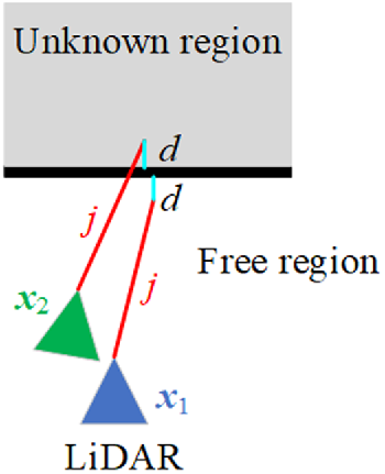
Measurement model decides how to correct odometry errors by LiDAR scan. As a typical representation, likelihood fields model [Reference Thrun, Burgard and Fox30] computes the distance between a LiDAR point and its nearest obstacle in occupancy map without considering the beam direction. A key advantage of likelihood fields model is its smoothness, because small changes in the robot’s pose x t solely have slight effects on the resulting distribution p(z t,j | x t , m ). Moreover, only two dimensions (x, y) involved in precomputing make likelihood fields model lower computation and memory demand. In particular, we employ likelihood fields model over the visible space to diminish the effect of unknown regions on the distribution p(z t,j | x t , m ), as shown in Figure 3. When a LiDAR point falls into free region and unknown region respectively due to different candidate poses, it can provide a higher probability in free region but a small constant probability in unknown region. It is rational as LiDAR cannot see through walls and this visibility constraint will lower the risk of creating false positives. Generating process of likelihood fields model over the visible space is shown in Appendix A.
Although both the shortest distances of the LiDAR point to obstacle are d when the LiDAR locates at candidate pose x 1 and x 2, likelihood fields model over the visible space assumes that p(z j | x 1, m) represents higher probability than p(z j | x 2, m).

If a LiDAR point falls into free region, its probability p(z t,j | x t , m ) is given by a zero-centered Gaussian. Assume distance between this LiDAR point and its nearest obstacle in occupancy map is d min, we compute p(z t,j | x t , m ) using:
 \begin{align}{p}({{z}_{t,j}} | {\boldsymbol{x}_{t}, {m}}) = \mathrm{e}^{-\frac{\textit{d}_{\min }^{2}}{2{\unicode[Arial]{x03C3}} ^{2}}}\end{align}
where σ is the standard deviation and set to the nominal value of LiDAR’s range accuracy.
An occupancy map and its corresponding likelihood fields model over the visible space are shown in Figure 4(a)–(b). We can see that the free and occupied regions in occupancy map have been assigned their respective probabilities, while the probabilities are assumed to be small constant values in unknown regions. Precomputing likelihood fields allows us to evaluate CSM candidates with trivial lookup operations, which guarantees the computational efficiency.
(a) Occupancy map of a corridor. (b) Likelihood fields model over the visible space of (a). Brighter value indicates larger probability. (c) A raw LiDAR scan (red). (d) The LiDAR scan after outliers removing (yellow).

In addition, it is convenient and effective to remove outliers for example, dynamic obstacles, from raw LiDAR scan by introducing a distance threshold d_threshold, as illustrated in Figure 4(c)–(d). If d min of a LiDAR point is above d_threshold, this point will be removed and not used in subsequent CSM. As can be seen, a too-small d_threshold is prone to remove too many LiDAR points including inliers, which will have a negative impact on the performance of CSM and even result in a failure of CSM from lack of adequate inliers. A big enough d_threshold is also able to remove outliers for example, dynamic obstacles, but some outliers with large measurement noise will have a bigger chance to survive that may lead to many false positives degrading the performance of CSM. We set the value of d_threshold based on the “3σ” principle, namely, if the measurement accuracy of a LiDAR is 5 cm, we set d_threshold to 15 cm. Moreover, we perform uniform sampling at a certain ratio for the LiDAR scan to make CSM less susceptible to correlated noise in adjacent measurements [Reference Thrun, Burgard and Fox30]. These trimming operations not only reduce computation cost but also improve robustness of the pose tracking module.
4.3. CSM acceleration
Although the likelihood fields model and trimming operations in Section 4.2 reduce computation cost of evaluating a single CSM candidate, there are a multitude of candidates to be evaluated for taking account of three dimensions (x, y, θ). It will be quite slow using brute force method directly and the real-time demand will not be supplied.
We select Computing 2D Slices method, not the faster Multi-Level Resolution method presented in ref. [Reference Olson14], to accelerate CSM evaluation process in consideration of the two following reasons. On the one hand, uncertainty of pose tracking is local and confined to a small region near the robot’s true pose. So only small search windows in three dimensions (x, y, θ) are required and in this case, Computing 2D Slices method can meet real-time demand already. On the other hand, sufficient candidates and the corresponding probabilities are required to compute covariance matrix
 $\sum _{{\boldsymbol{x}_{\textit{t}}}}$
. However, Multi-Level Resolution method will ignore a lot of candidates leading to only a partial candidates being evaluated, which is bad for the estimation of uncertainty.
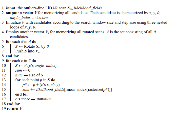
In practice, our implementation of Computing 2D Slices method is shown in Appendix B. At first, rotate the outliers-free LiDAR scan S m by all θ candidates to generate corresponding scans. In the process of evaluating candidates one by one, find the corresponding scan S properly rotated in advance according to θ and then, only simple translation operations are needed to move S to perform the final evaluation. We can realize that the nature of this method is to reduce rotation operations for LiDAR points to save computation time.
Fusion of x m and its neighbor candidates.

The candidate x m with the highest probability can be selected as global maximum after all candidates have been evaluated, as shown in Eq. (2). But it is restricted by the search step size. To alleviate this problem, we integrate over four neighbor candidates around x m to compute the final result x *, as shown in Figure 5. The eight neighbor candidates around x m are partitioned into four regions, and we decide the region in which true pose x may locate based on the probability difference between x m and its neighbor candidates:
 \begin{align}\text{ Region}(\boldsymbol{x})= \begin{cases} {p}_{m}-{p}_{u}\lt {p}_{m}-{p}_{d} \begin{cases} {p}_{m}-{p}_{r}\lt {p}_{m}-{p}_{l}\colon \mathrm{A}\\ {p}_{m}-{p}_{r}\gt {p}_{m}-{p}_{l}\colon \mathrm{B} \end{cases} \\[7pt] {p}_{m}-{p}_{u}\gt {p}_{m}-{p}_{d} \begin{cases} {p}_{m}-{p}_{r}\gt {p}_{m}-{p}_{l}\colon \mathrm{C}\\ {p}_{m}-{p}_{r}\lt {p}_{m}-{p}_{l}\colon \mathrm{D} \end{cases} \end{cases}\end{align}
where p m is the probability of x m , and probabilities of other neighbor candidates are denoted in a similar fashion.
When the region is identified, a weighted fusion of the corresponding four candidates will be carried out to obtain the estimation result x *:
 \begin{align}\boldsymbol{x}^{*} = \frac{\sum _{\textit{i}=1}^{4}\boldsymbol{x}_{i}\cdot \textit{p}_{i}}{\sum _{\textit{i}=1}^{4}\textit{p}_{i}}\end{align}
Actually, we attempted to fuse x m and its all eight neighbor candidates but the result was not as good as that using four candidates. Additionally, this fusion does not take into account θ dimension, because all candidates shown in Figure 5 are from the same angle slice.
Finally, x * will pay compensation to the predictive pose T p to provide the corrected pose T c by CSM:
 \begin{align}\boldsymbol{T}_c = \boldsymbol{T}_p + \boldsymbol{x}^*\end{align}
4.4. Low-pass filter
To mitigate the problem of undetermined sensor motion, a low-pass filter was applied in refs. [Reference Jaimez, Monroy and Gonzalez-Jimenez39] and [Reference Jaimez, Monroy, Lopez-Antequera and Gonzalez-Jimenez41]. Inspired by their work, we also employ a low-pass filter to improve precision and smoothness of the pose tracking module. With all evaluated candidates, we can obtain the covariance matrix
 $\sum _{{\boldsymbol{x}_{\textit{t}}}}$
by Eq. (4). Eigenvalues of
 $\sum _{{\boldsymbol{x}_{\textit{t}}}}$
will be computed and analyzed to detect which components of the motion are undetermined and which are well constrained. The corrected pose
T
c
provided by Eq. (10) is weighted with the predictive pose
T
p
to obtain the filtered pose
T
l
:
 \begin{align} \left[(1 + k_p)\boldsymbol{I} + k_{e}\boldsymbol{E}\right]\boldsymbol{T}_l = \boldsymbol{T}_c + \left(k_p\boldsymbol{I} + k_e\boldsymbol{E}\right) \boldsymbol{T}_p\end{align}
where
E
is a diagonal matrix containing the eigenvalues of
 $\sum _{{\boldsymbol{x}_{\textit{t}}}}$
, k
p
, k
e
are parameters of the filter and
I
is the identity matrix. In fact, k
p
imposes a constant weighting between
T
c
and
T
p
that helps to soften the estimated trajectory, while k
e
defines how the eigenvalues affect the final estimation. A high value of k
e
indicates that those pose terms with uncertainty will be approximated to their predictive value, whereas the corrected estimate will have a higher importance if k
e
is low. With respect to the selection of k
p
and k
e
, we aim to make (1 + k
p
)
I
and k
e
E
in Eq. (11) in the same order of magnitude by observing the eigenvalues of
 $\sum _{{\boldsymbol{x}_{\textit{t}}}}$
in advance. Then a grid search over them is performed to determine the optimal settings. Specifically, we set k
p
= 0.5 and k
e
= 5000 that provide us with good results in the experiments. In our implementation, only two dimensions (x, y) participate in Eq. (11), because we find a bit of decrease in repeated precision with θ dimension involved. So we only use “+” instead of the compound operator “
 $\oplus$
” in Eq. (11).
As a postprocessing step after CSM, the low-pass filter contributes to more precise and smoother pose estimation, which is important for planner decision to avoid violent corrective control actions. It is compact and trivial to implement but exhibits a good enough behavior owing to the dynamic smoothing.
5. Global localization
Compared to pose tracking, global localization requires the complete search space to help robot recover from unknown initial pose or unexpected localization failure at run time. The resulting numerous candidates make it crucial to reduce the volume to be evaluated to increase the efficiency of global localization. In this section, we will firstly give an overview of branch-and-bound method which can massacre many impossible candidates. Then a coarse-to-fine scheme is introduced to trade off efficiency and accuracy of the global localization module. At the end, we design some trigger criteria to detect localization failures.
5.1. Branch and bound
The branch-and-bound method was utilized to conduct real-time loop closure detection in ref. [Reference Hess, Kohler, Rapp and Andor16], which can quickly identify areas that may contain global maximum. There exists a common characteristic between loop closure detection and global localization: a large search window results in vast candidates that will spend much time. Therefore, we leverage branch-and-bound method to solve the global localization problem quickly and accurately.
The main idea of branch-and-bound is to represent subsets of possibilities as nodes in a tree where each leaf node represents a candidate. By partitioning the nodes and comparing current optimal solution with the remaining nodes, a large part of the tree will be pruned to save computation time. In the global localization module, branch-and-bound with depth-first search (DFS) method is employed to improve efficiency. We refer to [Reference Hess, Kohler, Rapp and Andor16] for more details on this method.
(a)–(d): Precomputed grids corresponding to height of 0, 2, 4, 6 respectively. Brighter value indicates larger probability.

To efficiently compute the upper bound, the precomputed grids
 $M^{h}_{precomp}$
are obtained in advance by the likelihood_fields presented in Section 4.2, where h (h = 0, 1, 2, …, hm) stands for height in the tree structure. Generating process of
 $M^{h}_{precomp}$
is shown in Appendix C. Figure 6 illustrates precomputed grids derived from the likelihood_fields shown in Figure 4(b). Let c
h
be a node at height h combining up to 2
h
× 2
h
leaf nodes. Thanks to each grid in
 $M^{h}_{precomp}$
storing the maxima of 2
h
× 2
h
grids in likelihood_fields beginning there, score of c
h
is exactly the maxima (upper bound) that the candidates covered by c
h
can reach, namely:
 \begin{align} score(c_{h}) & = \sum _{\textit{i}=1}^{\textit{N}}\textit{M}_{\textit{precomp}}^{\textit{h}}(\boldsymbol{T}_{\textit{g},\textit{ch}}\oplus \boldsymbol{s}_\textit{i})\\ & = \sum _{\textit{i}=1}^{\textit{N}}\max _{\textit{j}\in \textit{W}_{\textit{ch}}} \textit{likelihood}\textit{_ }\textit{fields}(\boldsymbol{T}_{\textit{g},\textit{j}}\oplus \boldsymbol{s}_\textit{i}) \nonumber\\[3pt] &\geq \max _{\textit{j}\in \textit{W}_{\textit{ch}}}\sum _{\textit{i}=1}^{\textit{N}}\textit{likelihood}\textit{_ }\textit{fields}(\boldsymbol{T}_{\textit{g},\textit{j}}\oplus \boldsymbol{s}_\textit{i}) \nonumber \end{align}
where
 $\boldsymbol{T}_{\textit{g},\textit{ch}}$
is the recovered pose implied by c
h
,
s
i
represents a LiDAR point (i = 1, 2, 3, …, N),
 $\textit{W}_{\textit{ch}}$
represents the candidates set covered by c
h
,
 $\boldsymbol{T}_{\textit{g},\textit{j}}$
is the recovered pose implied by a candidate in
 $\textit{W}_{\textit{ch}}$
(j = 1, 2, 3, …, 2
h
× 2
h
),
 $M^{h}_{precomp}$
(·) and likelihood_fields(·) are the evaluation functions based on precomputed grids
 $M^{h}_{precomp}$
and likelihood_fields respectively. Eq. (12) allows us to quickly narrow the scope that may contain global maximum and guarantees we will not miss maxima.
There exist two points to emphasize. On the one hand, the raw LiDAR scan S r instead of the outliers-free LiDAR scan S m should be used to match against the precomputed grids, as shown in Figure 1. This is because localization failures will result in many inliers removed such that CSM may fail to work with S m . On the other hand, it is necessary to rotate S r by all θ candidates in advance, like the operation in Section 4.3, to reduce rotation operations in CSM to achieve a higher efficiency.
5.2. Coarse-to-fine scheme
We employ a coarse-to-fine scheme to trade off efficiency and accuracy of the global localization module. At first branch-and-bound method is carried out with a relatively large angular search step, for example, 1°, in the complete search window to quickly find a coarse robot pose T g, c . Then, we regard T g, c as predictive pose to perform a further pose refinement using method described in Section 4 with smaller search steps and search windows to obtain a finer robot pose T g . Parameters we adopt are listed in Table 1, where r is occupancy map resolution.
Parameters for coarse-to-fine scheme.

There are two cases where global localization is required: unknown initial pose and unexpected localization failure at run time. In the first case, we directly adopt map size as linear search window and 360° as angular search window to perform global search. In another case, localization failures caused by disturbances such as uneven ground or collision may not lead to a large drift from correct pose, and the pose before localization failure is accessible to play the role of initial guess. Therefore, we adopt relatively small search windows, for example, 2 m for linear search window and 180° for angular search window, to perform a local search firstly. If the local search fails to retrieve correct pose, a global search will follow to fulfill the localization task.
In addition, there may be a large area of unknown regions in occupancy map as shown in Figure 7, where the robot is impossible to reach. If a subregion covered by a node locates at unknown regions, for example, subregion A or B, we will discard this node to accelerate global pose search. In practical, unknown grids number M unknown and occupied grids number M occupied in each subregion are recorded when generating precomputed grids. Given that:
There is a large area of unknown regions (gray) in the occupancy map. The red squares represent subregions covered by nodes at a certain height.

 \begin{align}M_{unknown} + M_{occupied} \gt \alpha \times M_{total}\end{align}
the corresponding node will be discarded. M
total
is total grids number in the subregion and
 $ \alpha$
is a coefficient. Obviously, a smaller
 $ \alpha$
is prone to prune more nodes making the search faster. But more free grids will be consequently ignored and the optimal solution may be missed, for example, in subregion C or D. We set
 $ \alpha$
to 0.9 empirically to obtain a good performance in the experiments.
5.3. Trigger criteria
Determining when to trigger global localization is an important problem. Manual supervision is a common and reliable method while this may be impractical at run time. The robot should be able to make a decision based on some estimates of localization performance. In regard to our method, measurement probability p( z t | x m , m ) of the global maximum x m is a valid indicator. If p( z t | x m , m ) is below a given threshold csm_lowest_score, for example, 0.6, we deem the robot encounters a localization failure and global localization should be triggered. However, thanks to the outliers removing step before CSM as shown in Figure 1, the remaining LiDAR points will locate at occupied regions or the surrounding areas even if there is a localization failure. As a result, p( z t | x m , m ) may be still greater than csm_lowest_score and global localization will not be triggered in time. To make our method more sensitive to localization failures, the removal ratio of LiDAR points R p is employed which is also an effective helper. After outliers removing step, if R p exceeds a given threshold csm_highest_ourliers_remove_ratio, for example, 0.6, we deem that a localization failure occurs and global localization should be triggered, as shown in Figure 8(a)–(b).
(a) The raw LiDAR scan (red) when the robot encounters a localization failure. (b) The remaining LiDAR points (yellow) after outliers removing. The measurement probability p(z t | x m, m) is 0.6368 that is greater than csm_lowest_score. So just relying on p(z t | x m, m) is not enough to trigger global localization in time. Nevertheless, the removal ratio Rp is 0.66 which is greater than csm_highest_ourliers_remove_ratio. Therefore, global localization will be triggered providing Rp is considered. (c) Two people are examining data beside the robot and block a large portion of LiDAR scan. (d) The raw LiDAR scan (red) in (c) scenario. (e) The remaining LiDAR points (yellow) after outliers removing. Although the robot has been properly located, global localization is still triggered due to a Rp of 0.79.

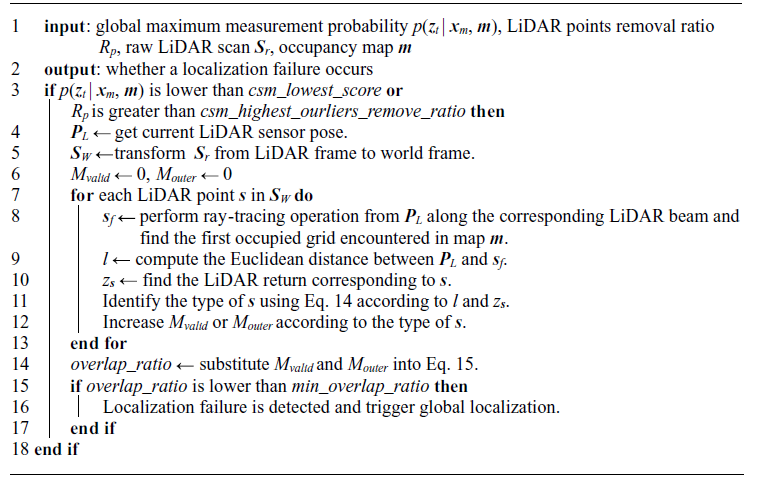
Another problem may come up with consideration of R p : global localization is triggered by mistake due to a large R p caused by dynamic obstacles, while the robot is properly located, as shown in Figure 8(c)–(e). To solve this problem, we divide raw LiDAR points into three types: valid point, outer point, and inner point, as shown in Figure 9. For a certain LiDAR point s i , we perform ray-tracing operation along the corresponding LiDAR beam to search for the first occupied grid s f encountered in occupancy map and compute distance l i between s f and LiDAR. Type of s i can be identified by comparing l i with the corresponding LiDAR return z t,i :
(a) Localization failure results in a large Rp, and a small overlap_ratio is obtained that will trigger global localization. (b) The robot has been properly located and dynamic obstacles result in a large Rp. However, there is a large overlap_ratio so that global localization will not be triggered.

 \begin{align}\text{Type}(\boldsymbol{s}_{i})=\begin{cases} {valid\ point}, \quad \left| z_{t,i}-l_{i}\right| \lt {d}\_ {threshold}\\[3pt] {outer\ point}, \quad z_{t, i} - l_{i} \geq {d}\_ {threshold}\\[3pt] {inner\ point}, \quad z_{t,i} - l_{i }\leq -{d}\_ {threshold} \end{cases}\end{align}
where d_threshold is the outliers removing threshold mentioned in Section 4.2.
After types of all LiDAR points have been identified, we count the valid point number M valid and the outer point number M outer . The reason why we ignore inner point is that it is not certain which, localization failure or dynamic obstacle, should be responsible for generation of the inner points, as shown in Figure 9. Then a new indicator overlap_ratio is defined as follows:
 \begin{align}\textit{overlap}\textit{_ }\textit{ratio }=\frac{M_{valid}}{M_{valid }+ M_{outer}}\end{align}
If overlap_ratio is below a given threshold min_overlap_ratio, we deem a localization failure occurs and global localization should be triggered. A big min_overlap_ratio makes it frequent to trigger global localization which may be unnecessary in some cases. For example, relatively low overlap_ratio caused by wheel slip or motion distortion does not mean a localization failure, which can be corrected by the pose tracking module gradually and does not require global localization. Frequent trigger of global localization consuming more time will impact the real-time performance, which may lead to the delay in pose estimation. A small min_overlap_ratio means the global localization is triggered only if an obvious enough localization failure occurs. It may be dangerous for the mobile robot if it cannot detect the localization failure in time and keeps running. After a search test over min_overlap_ratio in the range of [0.1, 0.2, 0.3, …, 0.9], we set its value to 0.5 that guarantees our localization system can detect localization failures in time and lower unnecessary alarms at the same time. The detection process is shown in Appendix D.
6. Experiments
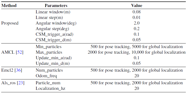
To validate the proposed localization method, we conduct extensive experiments in simulated environment, public datasets and real scenarios. Simulated experiments are carried out in Gazebo [50] simulation environment, where ground truth of the robot pose is available. Pre-2014 Robotics 2D-Laser Datasets [51] are used for the dataset-based experiments. Furthermore, we select three scenarios to conduct real experiments: an office building, a long corridor, and a workshop. Occupancy maps used in the experiments are built by KartoSLAM [Reference Konolige, Grisetti, Kümmerle, Burgard, Limketkai and Vincent15] with a resolution 2 cm. Primary comparison in this section is done among four methods: the proposed method, AMCL [52], Emcl2 [Reference Ueda, Arai, Sakamoto, Kikuchi and Kamiya36] and Als_ros [Reference Akai23]. Key parameters for all compared methods are listed in Table 2. We increase the particles number of the three compared methods in the global localization experiments to improve their recovery capacity. We implement the proposed method in C++ and all tests run on an Intel Core i5-7400 desktop computer with 8 GB RAM.
Key parameters for the compared methods.

6.1. Gazebo simulation
We construct a factory workshop with a size of 50 m × 50 m in Gazebo where machining centers, milling machines, drilling machines, gear cutting machines, forklift trucks, pallet trucks, workers and dumpsters are included, as shown in Figure 10(a). A virtual robot equipped with odometer and 2D-LiDAR is created to collect data. For the virtual 2D-LiDAR, its maximum range is 30 m and the range measurements are corrupted by Gaussian noise with a standard deviation of 0.02m. It runs at 40 Hz and has a field of view of 180° with an angular resolution 0.25°.
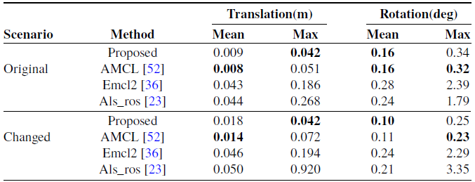
Localization errors in simulation experiments.

(a) The factory workshop created in Gazebo. (b) The robot movement path in original factory workshop whose total length is about 392 m. The blue star and black star represent start point and end point, respectively. (c) The changed factory workshop and the red circles highlight some changes. (d) The robot’s movement path in changed environment whose total length is about 367 m.

6.1.1. Pose tracking experiments
We build the occupancy map of the factory workshop firstly and then drive the virtual robot in this simulation environment at a maximum velocity of 1.0 m/s to collect sensor data. In addition, factory workshop is a typically dynamic scenario, where workers may frequently walk around and positions of pallet trucks may often change. To simulate these situations, we move all workers, pallet trucks and others and add some extra workers to the simulation environment, as shown in Figure 10(c). Then we recollect sensor data in the changed environment but perform localization tests with original occupancy map.
Thanks to the available ground truth, performance metric used in this experiment is the absolute trajectory error (ATE) [Reference Sturm, Engelhard, Endres, Burgard and Cremers53], including mean and max of absolute translation and rotation errors. Table 3 reports the localization errors of each method. Better results are highlighted in bold. Overall, the proposed method performs on par with AMCL and both present good enough performances. Even in changed environment, the mean translation errors are still less than the map resolution 2 cm. Their similar performances can be attributed to the noise-free odometry data in Gazebo. Accuracies of Emcl2 and Als_ros are a little worse because they update poses at a certain frequency, not based on translational and angular threshold for the odometry increment, therefore benefit less from the noise-free odometry data.
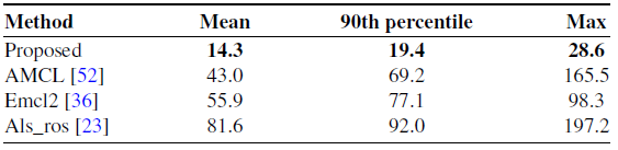
With regard to computational cost, we record 1000 consecutive pose update time for each method in the original simulation environment whose mean, 90th percentile and maximum are listed in Table 4. It is obvious that the proposed method is the most efficient, and most runtime below 20 ms is enough for indoor mobile robots which usually run at low velocities. Although the time complexity of all methods is O(n), where n is the candidates number, the pre-rotation for scan enables our method to be the most efficient one even if the candidates number (9*9*11 = 891) is more than other methods’ (500) as shown in Table 2.
Runtime comparison in simulation experiments (ms).

6.1.2. Global localization experiments
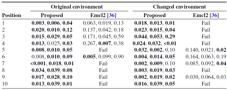
To validate the proposed global localization module, we collect sensor data at ten arbitrary positions in original and changed simulation environment respectively and then set initial pose to zero to simulate localization failure, as shown in Figure 11. If a correct pose cannot be recovered in 30 s, we deem this global localization fails. Table 5 reports the global localization pose error in the form of (
 $\Delta$
x,
 $\Delta$
y,
 $\Delta\theta$
). As it can be seen from the table, max error is 0.053 m in both X and Y dimensions and 0.29° in
 $\theta$
dimension at position 3 in the changed environment with the proposed method, which is accurate enough for global localization. Moreover, we do not trigger global localization manually, but use our trigger criteria proposed in Section 5.3 to detect localization failures autonomously. Emcl2 can recover a partial poses but exhibits an unstable behavior. These successful recoveries are only obtained by manually triggering its global localization service several times. AMCL and Als_ros cannot retrieve any correct pose because there are not new measurements fed to them so the corresponding results on them are not provided.
Ten arbitrary positions (1-10) in (a) original environment and (b) changed environment. Position 0 represents map origin. (c) LiDAR scan (red) at position 1 in original environment is mapped to the occupancy map by mistake before global localization. (d) Correct pose of position 1 has been recovered successfully by the proposed global localization method.

Global localization errors in simulation experiments (m, m, deg).

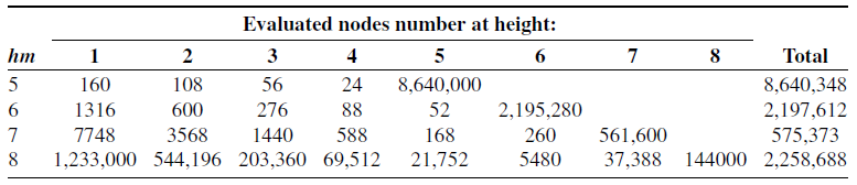
Time spent on global localization at each test position with the proposed method is shown in Table 6. We can see that the recovery time of most test positions is below 1 s, which is a satisfying performance. In particular, position 10 in the original scenario costs 4.3 s for its recovery. The number of its evaluated nodes reaches up to 2258688, while the maximal number among the other nine positions is only 318828. This is because the max height hm = 8 makes the nodes at this height too ambiguous at position 10, hence leading to more false positive nodes to be evaluated. In addition, max heights hm of the tree structure used by the branch-and-bound method are different in the two scenarios, whose effect on global localization efficiency will be discussed in Section 6.4. We do not record the time of Emcl2 for its several manual triggers.
Time spent on global localization with the proposed method in simulation experiments (s).

6.2. Experiments on public datasets
In this subsection, we select the Intel Research Lab and ACES Building datasets to validate the compared methods, as shown in Figure 12.
(a) The Intel Research Lab. (b) The ACES Building. For each dataset, the red line represents movement path of the mobile robot. Total distance the mobile robot has traveled is about 656 m in the Intel Research Lab and 331 m in the ACES Building.

6.2.1. Pose tracking experiments
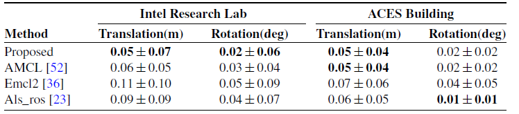
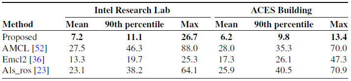
We build the occupancy maps with the two datasets and then execute all methods on the maps using the two datasets again. The benchmark proposed in ref. [Reference Kümmerle, Steder, Dornhege, Ruhnke, Grisetti, Stachniss and Kleiner54] serves as the performance metric in this subsection, which compares the error in relative pose changes to manually aligned ground truth relations. The experiment results are listed in Table 7. Better results are highlighted in bold. We can see that the proposed method outperforms other methods overall. In addition, the performances of Emcl2 and Als_ros are a little worse, which is consistent with that in the simulation experiments. Table 8 presents the runtime of all methods obtained in the same way as simulation experiments, indicating the highest efficiency of the proposed method.
Localization errors in experiments on public datasets.

Runtime comparison in experiments on public datasets (ms).

6.2.2. Global localization experiments
We select ten arbitrary positions in the two datasets respectively to validate the proposed global localization module in the same way as simulation experiments, as shown in Figure 13. Time spent on global localization at each test position with the proposed method is presented in Table 9. As can be seen, the proposed method achieves highly efficient global localization and that the recovery time of most test positions is below 1 s. Moreover, there is a similar efficiency in the two datasets although size of the ACES Building is larger than that of the Intel Research Lab. This is because there is a large area of unknown regions in the map of the ACES Building. Many impossible nodes in these regions will be discarded in advance based on Eq. (13), resulting in a higher global localization efficiency. Other methods fail to recover any correct pose because there is only a single scan for each test position, while they need more new measurements to distinguish where the robot is gradually.
6.3. Experiments in real environments
We use a holonomic mobile robot with four mecanum wheels, as shown in Figure 14(a), to collect sensor data. The robot is equipped with a Hokuyo UTM-30 LX LiDAR which runs at 40 Hz and has a field of view of 270° (we only utilize 180° in fact) with an angular resolution 0.25°. A cross laser pointer is fixed in front of the robot to indicate whether the robot reaches a target position. We select three scenarios: a sitting room, a long corridor, and a workshop, as shown in Figure 14(c)–(h). Sitting room is a typical application scenario for mobile robots, for example, cleaning robots. For the long corridor, there exist many similar features posing challenges to scan matching and the smooth floor will deteriorate odometry data as well. The workshop is also a typical scenario where more and more mobile robots, for example, automatically guided vehicle, are deployed to improve work efficiency and automation.
Time spent on global localization with the proposed method in experiments on public datasets (s).

Ten arbitrary positions (1-10) in (a) the Intel Research Lab and (b) The ACES Building. Position 0 represents map origin.

(a) The mobile robot we used in the experiments. (b) The red cross from laser pointer aligns with the green cross landmark on the floor indicating that the robot has reached this target position. Occupancy maps generated in (c)-(d) a sitting room, (e)-(f) a long corridor, and (g)-(h) a workshop. For each scenario, the red line represents movement path of the mobile robot. Position 0-3 stands for four target positions. Total distance the mobile robot has traveled is about 264 m in the sitting room, 1175m in the corridor, and 650 m in the workshop.

6.3.1. Pose tracking experiments
Thanks to the inaccessible ground truth in real environment, ATE cannot be obtained to evaluate localization performance. In this subsection, we employ the more accessible repeated localization precision (proximity of all estimated poses at the same position) as the performance metric. Concretely, we arbitrarily select four target positions in each scenario as shown in Figure 14(c)–(h). Cross landmarks are used to mark these target positions on the floor. When the robot reaches a certain target position, the cross from laser pointer maybe misaligned to the corresponding cross landmark due to localization errors. Then, we will manually adjust the robot with great caution to make them coincident. By this way, the robot is considered to reach this target position exactly and the estimated pose from localization method will be recorded, as shown in Figure 14(b). We repeat this process ten times for each target position. Additionally, to verify the low-pass filter of Eq. (11), we remove it from the proposed method and refer to this approach as proposed naive.
Figure 15 depicts the localization results of the proposed method at four target positions in sitting room. Maximum differences in each dimension among all estimated poses at each position are regarded as repeated localization precision. All results have been summarized in Table 10. Better results at each position are highlighted in bold. As it can be seen from the table, the proposed method and Emcl2 achieve similar repeated localization precisions most of which are less than 2 cm both in X and Y dimensions. However, maximum difference of Emcl2 is 4.2 cm at position 3 in corridor while ours is 2.4 cm at position 3 in workshop. There is a bit decrease in repeated localization precision with the proposed naive method, which is more obvious in corridor. The other two methods exhibit relatively poor precision behaviors. In terms of θ dimension, all methods present poor performances that maximum difference at each target position is relatively large overall (larger than 1°). This is because manual adjustment cannot guarantee the robot rotates in the same direction every time and is prone to result in a difference in heading. Some jitters in the estimated trajectory may occur without the help of low-pass filter, as shown in Figure 16, which will have a bad effect on the controller performance and bring potential safety hazards to mobile robots. In the same way as simulation experiments, we record 1000 consecutive pose update time for each method in all scenarios and summarize the results in Table 11. We can observe that the proposed method requires lower computational cost most of which are less than 20 ms, so the real-time demand can be met. On the whole, our method presents high enough performances both in precision and efficiency and outperforms other compared methods.
localization results of the proposed method at four target positions in the sitting room.

Repeated localization precision in real experiments.

Runtime comparison in real experiments (ms).

Trajectories in (a) the sitting room, (b) the long corridor, and (c) the workshop.

Four arbitrary positions before and after global localization with our method in A1-A8 the sitting room, B1-B8 the corridor, and C1-C8 the workshop.

6.3.2. Global localization experiments
To validate our global localization module in real environments, we collect sensor data at four arbitrary positions in each scenario and then set initial pose to zero to simulate localization failure. Compared to a still robot in the simulation experiments, we drive the robot to perceive new measurements allowing all methods to distinguish where it is gradually in this subsection. However, the proposed method utilizes only a single scan in fact. Furthermore, all methods carry out global localizations autonomously without any manual trigger. We solely demonstrate qualitative results from lack of ground truth, as shown in Figure 17. Time spent on global localization at each test position is listed in Table 12. As can be seen, all correct poses have been recovered quickly from localization failures with our global localization method even in the ambiguous cases of position B1, B2, and B4. A partial test positions have found their correct poses with the help of AMCL, but it takes much longer time than our method. In addition, it is difficult for AMCL to retrieve correct poses in the ambiguous cases of position B1, B2, and B4. In face of such localization failures, the other two methods exhibit poor behaviors even if new measurements have been fed to them.
Time spent on global localization in real environments (s).

Time spent on global localization in each scenario using different max heights hm.

6.4. Experiments on the max height
From foregoing global localization experiments, we notice that the max heights hm of the tree structure used by the branch-and-bound method are different in different scenarios to obtain the optimal convergence speed. It is a key parameter influencing global localization efficiency so we discuss it here.
We test the selected positions in each scenario using different max heights and record the corresponding time cost. All results are shown in Figure 18. We only present some applicable max heights for each scenario because other smaller or larger max heights will lead to much slower convergence speed.
Assume a map size is M×N, the angular search window size and search step size are 360° and 1° respectively. The nodes at the max height level, whose number is
 $\frac{\textit{M}\times \textit{N}}{2^{\textit{hm}}\times 2^{\textit{hm}}}\times \frac{360}{1}$
, will not be pruned and will be evaluated one by one. Therefore, smaller hm will induce more nodes at the max height taking up most of the time in one global localization, as shown in Table 13 when hm = 5 or 6. Increasing hm will decrease the evaluated nodes number at the max height. But the pruning efficiency at other height may decrease at the same time, which lowers the global localization efficiency in consequence, as shown in Table 13 when hm = 8. This is because large hm is prone to make the nodes at this height more ambiguous, which means the search process can spend large amounts of exploration time in poor regions of the search space and DFS can choose many long, bad paths before it explores a path leading to an optimal solution [Reference Morrison, Jacobson, Sauppe and Sewell55].
Evaluated node number at each height using different max heights at position 10 in original simulation factory.

7. Conclusion and future work
This paper has presented a 2D-LiDAR and occupancy map-based localization method for indoor mobile robots using CSM, which includes a pose tracking module and a global localization module. The former utilizes CSM within a small search space to correct accumulated odometry errors. A low-pass filter associating the predictive pose from odometer with the corrected pose by CSM is applied to improve precision and smoothness of the pose tracking module. The latter utilizes CSM within the complete search space to help robot recover from unknown initial pose or unexpected localization failure at run time. The branch-and-bound method is employed to improve search efficiency substantially. Moreover, several trigger criteria have been designed carefully to enable our method to detect localization failures in time. We have validated the proposed method by conducting simulated, public datasets-based and real experiments and shown its good performance on both pose tracking and global localization. However, the global localization efficiency will decrease with the increase of the map size. So, we plan to develop a new method to handle this problem in the future.
Author contributions
Song Du conceived and designed the study. Song Du, Tao Chen, and Zhonghui Lou conducted data gathering. Song Du performed statistical analyses and wrote the article. Tao Chen and Yijie Wu reviewed the article.
Financial support
This work was supported by the National Natural Science Foundation of China (Grant No.51275462).
Competing interests
The authors declare no conflicts of interest exist.
Ethical approval
Not applicable.
Appendix A
Precompute likelihood fields model over the visible space

Appendix B
Computing 2D slices method for CSM acceleration

Appendix C
Generating process of the precomputed grid based on likelihood_fields. Assume h = 2, each node at this height combines up to 22 × 22 candidates. A sliding window (red squares) covering a subregion of 22 × 22 grids slides on likelihood_fields along X and Y direction in sequence to obtain the maxima in each subregion as the corresponding grid value in
 $M^{2}_{precomp}$
. Note that size of
 $M^{2}_{precomp}$
is 22 – 1 grids larger than likelihood_fields in both X and Y dimensions.

Appendix D
Detect localization failure