Nomenclature
- HGVs
-
hypersonic gliding vehicles
- GHGVs
-
group of hypersonic gliding vehicles
- MAS
-
multi-agent system
- RBFNNs
-
radial basis function neural networks
- UAV
-
unmanned aerial vehicle
- ETM
-
event-triggered mechanism
- SPFTS
-
semi-global practical fixed-time stability
- DITV
-
dynamic internal trigger variable
- GHCVs
-
group of hypersonic cruise vehicles
- GHBGVs
-
group of hypersonic boost-glide vehicles
- ADE
-
auxiliary differential equation
- EI
-
explosion of complexity
- FCF
-
fixed-time command filter
- DETM
-
dynamic event-triggered mechanism
1.0 Introduction
Nowadays hypersonic gliding vehicles (HGVs) have emerged as a significant research focus in aerospace engineering, driven by their capacity for multi-domain operations, superior manoeuverability across velocity regimes and mission-critical attributes including precision strike capabilities, extended operational ranges and hypersonic-speed performance [Reference Han, Guo, Ding, Cao, Wang, Han and Guo1, Reference Han, Hu and Xin2]. However, successive development of defense system has resulted in a significant reduction in the operational effectiveness and penetrating capability of single HGV. In the years to come, groups of hypersonic gliding vehicles (GHGVs) collaborate in a group format will be more compatible with saturation attacks and coordinated anti-jamming.
The basic theory for GHGVs formation flight is consensus control [Reference Sui, Bai, Tong and Chen3, Reference Sui, Bai, Tong and Chen4] for the multi-agent system (MAS). There is a lot of research from various perspectives, such as time varying formation control, adaptive neural network control [Reference Liu, Zhao, Liu, Li, Tong and Chen5] and distributed coordinated control [Reference Deng, Zhang, Qiu and Chen6]. While consensus control architectures have achieved notable success in small-scale unmanned aerial vehciles (UAVs) operating at subsonic regimes [Reference Imran, Kurtulus, Memon, Goli, Kouser and Alhems7], this control paradigm remains underutilised for HGV clusters due to three fundamental challenges:
-
1. Different from simple motion model of UAVs, the system dynamic equation of HGVs is fast time varying, highly nonlinear, strongly coupled and subjected to unknown inherent uncertainties.
-
2. In contrast to multi-UAV flying in formation, HGV cannot perform constant altitude and steady velocity. In the meantime, thrust considered to be unavailable means the energy dissipation process of a multi-HGV system is irreversible and has a single direction of motion.
-
3. Compared with UAV missions, HGVs usually glide in formation for a longer time. Although continuous time-based sampling can effectively ensure the real-time update of the control protocol, redundant sampling data may be generated, which will result in unnecessary information transmission and waste of system computing resources.
Hence, the pressing need to optimise communication resource utilisation while bolstering the control performance of GHGVs, amidst the intricate interplay of time sensitivity and internal uncertainties, stands as a pivotal research frontier and the driving force behind this paper.
Neural networks’ ability to approximate unknown functions has led to the development of several adaptive neural methods in recent years [Reference Yu, Dong, Li and Ren8, Reference Tan, Liu, Chen and Zhang9]. These strategies excel in handling multi-agent systems with uncertainties, outperforming traditional centralised control in practicality. Yet, they all rely on non-finite time for controller design, meaning convergence occurs as time approaches infinity. As is well-known, the convergence rate stands as a paramount benchmark for evaluating the proficiency of leader-follower consensus control in MAS. Among the elite methodologies designed to propel this rate, fixed-time technology has emerged as a preeminent solution, finding extensive application across various MAS. Distinct from finite-time technology, fixed-time technology exhibits an unparalleled capacity to dramatically accelerate the convergence rate of nonlinear MAS, transcending the limitations imposed by the initial states of both individual agents and their interconnected peers. Research on fixed-time tracking consensus for MAS of different orders is documented in Ref. (Reference He, Li and Meng10). Inspired by Ref. (Reference Zuo11), Fu and Wang [Reference Fu and Wang12] refined the control algorithm for second-order MAS, while Refs (Reference Liu, Wang, Li and Xu13, Reference Meng, Ma and Shi14) proposed fixed-time adaptive schemes for nonlinear systems. Additionally, Ref. (Reference Gong and Han15) investigated observer-based adaptive control for second-order MAS. These adaptive approaches significantly impact MAS control, but traditional methods only ensure convergence within an unknown interval near zero, making asymptotic stability challenging to achieve in nonlinear systems. What’s more, the above results stem from simplified dynamics models of MAS. Addressing the formation control of multiple high-altitude, long-endurance vehicles necessitates considering additional factors due to their unique flight dynamics and environments, such as high nonlinearity, unavailable thrust, rapidly changing velocities, non-affine properties and multi-source uncertainties. Given the promising findings from the prior analysis, it is crucial to devise a formation control algorithm for the GHGVs system that ensures rapid and highly precise fixed-time convergence.
It is imperative to note that the study proposes distributed fixed-time control protocols based on the time-triggered mechanism [Reference Yang and Dong16–Reference Hu, Wang, Cheng, Li, Liu and Chen18], an approach that inherently increases communication overhead and induces inefficient utilisation of communication resources. In contrast to time-triggered strategies, the event-triggered mechanism (ETM) incorporates predetermined trigger conditions to regulate data transmission necessity, thereby substantially reducing communication costs. This methodology demonstrates significant improvements in achieving consensus control for MAS [Reference Zhang, Xia and Ma19–Reference Salmanpour, Arefi and Cao21]. Notably, Zhan and colleagues devised a fixed-time static switching ETM controller tailored for nonlinear systems, leveraging radial basis functional neural networks (RBFNNs) to approximate unknown nonlinearities with precision [Reference Zhan, Wang, Guo, Wu and Li22]. Similarly, Zhu and his team concurrently engineered a finite-time distributed controller and an ETM for MAS, successfully implementing consensus tracking within the system [Reference Lu, Wu, Zhan and Yan23]. Wang et al. further delved into the consensus control of networked MAS, proposing a fixed-time ETM control strategy that incorporates a comparative threshold method to guarantee semi-global practical fixed-time stability (SPFTS) of the system [Reference Wang, Wang, Zhang, Du, Liu and Chen24]. These advancements demonstrate the superiority and efficiency of ETM over traditional time-triggered methods in the realm of MAS consensus control. Nevertheless, the aforementioned ETMs overlook the design of a dynamic internal trigger variable (DITV), resulting in suboptimal dynamic performance in threshold adjustment.
Based on the above theoretical research and engineering application value, the main challenge of developing a distributed consensus control protocol for GHGVs is the strong coupling of non-affine non-linear dynamic with hypervelocity characteristics and multi-source uncertainties. To address this problem, this paper presents a fixed-time dynamic event-triggered formation control framework. The crucial achievements can be stated as follows:
-
• Different from simple dynamic model of UAVs applied in Khodaverdian et al. [Reference Khodaverdian, Hajshirmohamadi, Hakobyan and Ijaz25], this is the first RBFNN-based fixed-time controller for GHGVs applying non-affine non-linear dynamic coupled with hypervelocity characteristics and multi-source uncertainties. The control model integrates a fixed-time command filter, auxiliary differential equation and adaptive uncertainty compensating laws.
-
• A novel adaptive distributed fixed-time control framework utilising DETM is devised for GHGVs under directed graphs. In contrast to Du [Reference Du, Liang and Xue26] and Cui [Reference Cui, Xu, Chen and Yu27], the control protocol designed in this paper can adaptively adjust the update frequency, exhibits faster convergence rate while conserving the communication resources.
-
• This paper outlines a design blueprint of distributed fixed-time adaptive controller based on dynamic event-triggered, presenting a versatile model applicable to both GHCVs and group of hypersonic boost-glide vehicles (GHBGVs).
2.0 Problem Formulation and Preliminaries
2.1 Hypersonic gliding vehicle model
By ignoring the rotation and curvature of the Earth, we describe the three-degree-of-freedom point-mass equations of re-entry flight phase for GHGVs as follows:
 \begin{align} \left\{\begin{array}{lll}{\dot{x}}_{i}={V}_{i}\mathrm{cos}{\theta }_{i}\mathrm{cos}{\sigma }_{i} {} {} \\ {\dot{y}}_{i}={V}_{i}\mathrm{sin}{\theta }_{i} {} {} \\ {\dot{z}}_{i}={V}_{i}\mathrm{cos}{\theta }_{i}\mathrm{sin}{\sigma }_{i} {} {} \\ {\dot{V}}_{i}=-\frac{{C}_{{D}_{i}}{\rho }_{i}{V}_{i}^{2}{S}_{i}}{2{m}_{i}}-g\mathrm{sin}{\theta }_{i} {} , {} \\ {\dot{\theta }}_{i}=\frac{{C}_{{L}_{i}}{\rho }_{i}{V}_{i}{S}_{i}\mathrm{cos}{\upsilon }_{i}}{2{m}_{i}}-\frac{g}{{V}_{i}}\mathrm{cos}{\theta }_{i} {} {} \\ {\dot{\sigma }}_{i}=\frac{{C}_{{L}_{i}}{\rho }_{i}{V}_{i}{S}_{i}\mathrm{sin}{\upsilon }_{i}}{2{m}_{i}\mathrm{cos}{\theta }_{i}} {} {} \end{array}\right.\end{align}
where
 $ i=0$
represents the HGV as a leader, and
 $ i=\mathrm{1, 2},\cdots ,K$
represent the HGVs as followers;
 $ {V}_{i}$
is the velocity;
 $ {\theta }_{i}$
is the flight path angle;
 $ {\sigma }_{i}$
represents the heading angle;
 $ {x}_{i},{y}_{i},{z}_{i}$
stand for the position in the ground coordinate system;
 $ {\upsilon }_{i}$
is the bank angle;
 $ {m}_{i}$
means the mass,
 $ {S}_{i}$
means the reference area; g represents the gravitational acceleration;
 $ {\rho }_{i}$
represents dimensional atmospheric density, denoted by
 $ {\rho }_{i}={\rho }_{0}{e}^{-\frac{{h}_{i}}{{H}_{MCP}}}$
, where
 $ {h}_{i}={y}_{i}$
,
 $ {\rho }_{0}=1.225$
,
 $ {H}_{MCP}=7100$
. The terms
 $ {C}_{{D}_{i}}$
and
 $ {C}_{{L}_{i}}$
are designated to denote the coefficients of lift and drag described as
 $ {C}_{{L}_{i}}={C}_{{L}_{i}}^{\alpha }{\alpha }_{i}$
,
 $ {C}_{{D}_{i}}={C}_{{D}_{i}}^{{\alpha }_{i}^{2}}{\alpha }_{i}^{2}+{C}_{{D}_{i}}^{{\alpha }_{i}}{\alpha }_{i}+{C}_{{D}_{i}}^{0}+{C}_{{D}_{i}}^{{\delta }_{e}}{\delta }_{e,i}$
, where
 $ {\delta }_{e,i}$
is the deflection angle of speed brake;
 $ {\alpha }_{i}$
is the angle-of-attack;
 $ {\upsilon }_{i}$
is the bank angle;
 $ {C}_{{L}_{i}}^{\alpha }$
,
 $ {C}_{{D}_{i}}^{{\alpha }_{i}^{2}}$
,
 $ {C}_{{D}_{i}}^{{\alpha }_{i}}$
,
 $ {C}_{{D}_{i}}^{0}$
, and
 $ {C}_{{D}_{i}}^{{\delta }_{e}}$
are known coefficients.
To ensure the validity of the established motion model,the following fundamental assumptions are introduced:
Assumption 1. The hypersonic vehicle cluster operates under a constrained flight duration not exceeding 300 seconds, and all vehicles maintain operational altitudes within the stratified atmospheric band of 20 kilometers to 60 kilometers throughout the mission profile.
Assumption 2. (quasi-equilibrium glide trajectory): It is postulated that all hypersonic vehicles within the cluster adhere to quasi-equilibrium glide trajectories throughout the flight phase under consideration. This implies that the cluster formation is subject to a strict altitude stability criterion that actively suppresses potential phugoid-mode oscillations or altitude skipping phenomena.
Assumption 3. The group of HGVs clusters is homogeneous, which indicates that each cluster possesses similar aerodynamic performance
Define state variables as
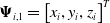 $ {\boldsymbol{\Psi }}_{i,1}={\left[{x}_{i},{y}_{i},{z}_{i}\right]}^{T}$
,
 $ {\boldsymbol{\Psi }}_{i,2}={\left[{V}_{i},{\theta }_{i},{\sigma }_{i}\right]}^{T}$
, control input as
 $ {\mathbf{u}}_{i}=\left[-{\delta }_{e,i},\right.{\left.{C}_{L,i}\mathrm{cos}{\upsilon }_{i},{C}_{L,i}\mathrm{sin}{\upsilon }_{i}\right]}^{T}$
, then the actual control signal can be inversely solved by (2)
 \begin{align} {\upsilon }_{i}=\mathrm{a}\mathrm{r}\mathrm{c}\mathrm{t}\mathrm{a}\mathrm{n}\left(\frac{{\mathbf{u}}_{{i}_{\left(3\right)}}}{{\mathbf{u}}_{{i}_{\left(2\right)}}}\right),{\alpha }_{i}=\frac{{\mathbf{u}}_{{i}_{\left(2\right)}}}{\mathrm{cos}{\upsilon }_{i}},{\delta }_{e,i}=\frac{-{\mathbf{u}}_{{i}_{\left(1\right)}}-\left({C}_{{D}_{i}}^{{\alpha }_{i}^{2}}{\alpha }_{i}^{2}+{C}_{{D}_{i}}^{{\alpha }_{i}}{\alpha }_{i}+{C}_{{D}_{i}}^{0}\right)}{{C}_{{D}_{i}}^{{\delta }_{e}}}\end{align}
Considering the effects of uncertainties and disturbances to which the system is subjected in engineering practice, we obtain the time-based non-affine nonlinear system:
 \begin{align} \left\{\begin{array}{lll}{\dot{\boldsymbol{\Psi }}}_{i,1}={\boldsymbol{\Pi }}_{i,1}\left({\stackrel{-}{\boldsymbol{\Psi }}}_{i,2}\right)+{\Delta }{\boldsymbol{\Omega }}_{i,1}\left({\boldsymbol{\Psi }}_{i,1}\right) {} {} \\ {\dot{\boldsymbol{\Psi }}}_{i,2}={\boldsymbol{\Xi }}_{i}\left({\stackrel{-}{\boldsymbol{\Psi }}}_{i,2}\right)+{\boldsymbol{\Pi }}_{i,2}\left({\stackrel{-}{\boldsymbol{\Psi }}}_{i,2},{\mathbf{u}}_{i}\right)+{\Delta }{\boldsymbol{\Omega }}_{i,2}\left({\boldsymbol{\Psi }}_{i,1}\right) {} , {} \\ {\omega }_{i}={\boldsymbol{\Psi }}_{i,1} {} {} \end{array}\right.\end{align}
where
 $ {\stackrel{-}{\boldsymbol{\Psi }}}_{i,j}={\boldsymbol{\Psi }}_{i,1},\cdots ,{\boldsymbol{\Psi }}_{i,j}$
;
 $ {\boldsymbol{\Xi }}_{i}$
is known nonlinear function;
 $ {\boldsymbol{\Pi }}_{i,1}$
and
 $ {\boldsymbol{\Pi }}_{i,2}$
are known non-affine items;
 $ {\Delta }{\boldsymbol{\Omega }}_{i,1}$
and
 $ {\Delta }{\boldsymbol{\Omega }}_{i,2}$
stand for unknown internal uncertainties;
 $ {\omega }_{i}$
is the system output of the
 $ i-th$
follower.
The following assumptions and lemmas are put forward, which will be utilised soon afterwards.
Assumption 4.
To avoid singularities, the flight path angle of HGVs should be at
 $ \left[0,\pi /2\right)$
.
Assumption 5.
For functions in non-affine form, there is positive lower bound
 $ \underset{-}{\Pi }$
and upper bound
 $ \stackrel{-}{\Pi }$
satisfying the following form
 \begin{align} 0 \lt \underset{\mathrm{}-\mathrm{}}{\Pi }{ \le }||\frac{\partial {\boldsymbol{\Pi }}_{i,j}\left({\stackrel{-}{\boldsymbol{\Psi }}}_{i,j+1}\right)}{\partial {\boldsymbol{\Psi }}_{i}}||{ \le }\stackrel{-}{\Pi } \lt \infty \end{align}
Lemma 1. [Reference Cui, Xu, Chen and Yu27] For any positive constants
 $ {p}_{1}$
,
 $ {p}_{2}$
and
 $ {\chi }_{a}$
, it produces
 \begin{align} {\left|{x}_{1}\right|}^{{p}_{1}}{\left|{x}_{2}\right|}^{{p}_{2}}{ \le }\frac{{p}_{1}{\chi }_{a}}{{p}_{1}+{p}_{2}}{\left|{x}_{1}\right|}^{{p}_{1}+{p}_{2}}+\frac{{p}_{2}{\chi }_{a}^{\frac{-{p}_{1}}{{p}_{2}}}}{{p}_{1}+{p}_{2}}{\left|{x}_{2}\right|}^{{p}_{1}+{p}_{2}},\end{align}
Lemma 2. [Reference Cui, Xu, Chen and Yu27] For any
 $ {x}_{2}\le {x}_{1}$
,
 $ {x}_{3}\ge 0$
,
 $ {x}_{4} \gt 0$
and
 $ p \gt 0$
, it yields
 \begin{align} \left\{\begin{array}{l}{x}_{2}^{1+p}-{x}_{1}^{1+p}{ \le }({x}_{1}-{x}_{2}{)}^{1+p}\\ {x}_{3}^{p}({x}_{4}-{x}_{3}){ \le }\frac{{x}_{4}^{1+p}-{x}_{3}^{1+p}}{1+p}\end{array}\right.\end{align}
Lemma 3. [Reference Polycarpou and Ioannou28] For any
 $ \zeta \gt 0$
and
 $ x\in \mathbb{R}$
, we have
 \begin{align} 0{ \le }\left|x\right|-x\,\mathrm{t}\mathrm{a}\mathrm{n}\mathrm{h}\left(\frac{x}{\zeta }\right){ \le }\iota \zeta \end{align}
where
 $ \iota $
is a constant satisfying
 $ \iota ={e}^{-(\iota +1)}$
,
 $ \iota =0.2785$
.
Lemma 4. [Reference Tong and Li29] For any
 $ x\in \mathbb{R},\mu \in {\mathbb{R}}^{+}$
, we have
 \begin{align} \left|x\right|-\frac{{x}^{2}}{\sqrt{{x}^{2}+{\mu }^{2}}}{ \le }\mu \end{align}
Lemma 5.
For any matrix
 $ \mathit{X}\in {\mathbb{R}}^{m\times 1}$
and positive parameter
 $ \tau $
meeting
 $ 0 \lt \tau \lt 1$
, there exists
 \begin{align} -\tau \mathbf{X}{ \le }\tau {\left[\left|{X}_{i,1}\right|,\left|{X}_{i,2}\right|,\cdots ,\left|{X}_{m,1}\right|\right]}^{T}\end{align}
2.2 Graph theory
In the MAS, a communication network between agents is described by a graph
 $ \mathcal{R}=\left(\mathcal{V},\epsilon ,\mathcal{A}\right)$
, where
 $ \mathcal{V}=\left\{\mathrm{1, 2},\dots ,n\right\}$
is set of nonempty nodes,
 $ \epsilon =\left\{\left({n}_{i},{n}_{j}\right)\right\}\in \mathcal{V}\times \mathcal{V}$
represents the set of edges,
 $ \mathcal{A}=\left[{a}_{ij}\right]\in {\mathbb{R}}^{n\times n}$
is adjacency matrix. If
 $ \left({n}_{i},{n}_{j}\right)\in \epsilon $
,
 $ {a}_{ij} \gt 0$
, then the agent
 $ i$
can pass information to agent
 $ j$
. If
 $ \left({n}_{i},{n}_{j}\right)\notin \epsilon $
, then
 $ {a}_{ij}=0$
. Assume that agents do not have access to information about themselves, which means
 $ {a}_{ii}=0$
. For undirected graphs, the adjacency matrix exhibits symmetry implying
 $ {a}_{ij}={a}_{ji} \gt 0$
. For directed graph, the adjacency matrix is asymmetric.
Definition 1.
If there exists a path between any two nodes
 $ {n}_{i}$
,
 $ {n}_{j}$
, the undirected graph
 $ \mathcal{R}$
is connected.
The degree matrix
 $ \mathcal{P}=diag\left({p}_{i}\right)\in {R}^{n\times n}$
of graph
 $ \mathcal{R}$
represents the sum of the outdegree and indegree of a node. Note that
 $ \mathcal{P}$
is a diagonal array and the diagonal elements are
 $ {p}_{i}=\sum _{j\in {N}_{i}}\,{a}_{ij},i=\mathrm{1, 2},\dots ,n$
. Define the Laplacian matrix as
 $ \mathcal{L}=\mathcal{P}-\mathcal{A}$
, we have
 \begin{align} {\mathcal{L}}_{ij}=\left\{\begin{array}{l@{\quad}l}\sum\limits _{j\in {n}_{i}}\,{a}_{ij},\,i=j {} \\[4pt] -{a}_{ij},i\ne j {} . \end{array}\right.\end{align}
Consider the information sharing between leaders and followers to be unidirectional, i.e. the leaders can pass information to the followers, but the followers’ information cannot influence the leaders. Define
 $ \mathcal{D}=diag\left({d}_{1},{d}_{2},\dots ,{d}_{n}\right)$
, note that
 $ {d}_{i}=1$
when followers can get information from the leader, otherwise
 $ {d}_{i}=0$
. Denote
 $ \mathcal{H}=\mathcal{L}+\mathcal{D}$
as the communication topology matrix, which represents the information transmission relation between leaders and followers. When at least one follower can get information from the leader and the undirected graph is connected,
 $ \mathcal{H} \gt \gt 0$
.
2.3 Fixed-time theory
Lemma 6. [Reference Cheng, Xin, Wang, Gan, He and Ding30] Regarding a dynamic system
 $ \dot{\Phi }\left(t\right)=\chi (\Phi ,t),\Phi \left(0\right)={\Phi }_{0}$
, if the Lyapunov function
 $ L\left(x\right)$
is positive definite meeting
 \begin{align} \dot{L}\left(x\right){ \le }-{c}_{1}L\left(x\right)-{c}_{2}{L}^{p}\left(x\right)-{c}_{3}{L}^{q}\left(x\right)+{\delta }_{a}\end{align}
where
 $ {c}_{1}$
,
 $ {c}_{2}$
,
 $ {c}_{3}$
are positive constants,
 $ 0 \lt {\delta }_{a} \lt +\infty $
,
 $ p$
and
 $ q$
are odd numbers meeting
 $ 0 \lt p \lt 1$
,
 $ q \gt 1$
. Then the system exhibits semi-global practical fixed-time stability, with the residual set of the solution fulfills
 \begin{align} x\in \left\{x\left|L\right(x){ \le }\mathrm{m}\mathrm{i}\mathrm{n}\left\{\frac{{\delta }_{a}}{(1-{{\Delta }}_{\epsilon }){c}_{1}}{\left(\frac{{\delta }_{a}}{(1-{{\Delta }}_{\epsilon }){c}_{2}}\right)}^{\frac{1}{p}}{\left(\frac{{\delta }_{a}}{(1-{{\Delta }}_{\epsilon }){c}_{3}}\right)}^{\frac{1}{q}}\right\}\right\}\end{align}
where
 $ {{\Delta }}_{\epsilon }$
is a constant satisfying
 $ 0 \lt {{\Delta }}_{\epsilon } \lt 1$
. Then the calculation of the settling time is performed as below
 \begin{align} {T}_{s}{ \le }\mathrm{m}\mathrm{a}\mathrm{x}\left\{\frac{\mathrm{l}\mathrm{n}\left(1+\frac{{c}_{1}}{{{\Delta }}_{\epsilon }{c}_{2}}\right)}{{c}_{1}(1-p)},\frac{\mathrm{l}\mathrm{n}\left(1+\frac{{{\Delta }}_{\epsilon }{c}_{1}}{{c}_{2}}\right)}{{{\Delta }}_{\epsilon }{c}_{1}(1-p)}\right\}+\mathrm{m}\mathrm{a}\mathrm{x}\left\{\frac{\mathrm{l}\mathrm{n}\left(1+\frac{{c}_{1}}{{{\Delta }}_{\epsilon }{c}_{3}}\right)}{{c}_{1}(q-1)},\frac{\mathrm{l}\mathrm{n}\left(1+\frac{{{\Delta }}_{\epsilon }{c}_{1}}{{c}_{3}}\right)}{{{\Delta }}_{\epsilon }{c}_{1}(q-1)}\right\}\end{align}
By utilising inequality
 $ \mathrm{l}\mathrm{n}(1+x) \lt x,x \gt 0$
, we obtain
 \begin{align} \left\{\begin{array}{lll}\mathrm{m}\mathrm{a}\mathrm{x}\left\{\frac{\mathrm{l}\mathrm{n}\left(1+\frac{{}_{1}}{{{\Delta }}_{\epsilon }{c}_{2}}\right)}{{c}_{1}(1-p)},\frac{\mathrm{l}\mathrm{n}\left(1+\frac{{{\Delta }}_{\epsilon }{c}_{1}}{{c}_{2}}\right)}{{{\Delta }}_{\epsilon }{c}_{1}(1-p)}\right\} \lt \frac{1}{{c}_{2}{{\Delta }}_{}(1-p)} {} {} \\ \mathrm{m}\mathrm{a}\mathrm{x}\left\{\frac{\mathrm{l}\mathrm{n}\left(1+\frac{{c}_{1}}{{{\Delta }}_{\epsilon }{c}_{3}}\right)}{{c}_{1}(q-1)},\frac{\mathrm{l}\mathrm{n}\left(1+\frac{{{\Delta }}_{\epsilon }{c}_{1}}{{c}_{3}}\right)}{{{\Delta }}_{\epsilon }{c}_{1}(q-1)}\right\} \lt \frac{1}{{c}_{1}{{\Delta }}_{\epsilon }(q-1)} {} {} \end{array}\right.\end{align}
According to the conclusion in Cheng [Reference Cheng, Xin, Wang, Gan, He and Ding30], the upper bound of settling time
 $ {\mathrm{T}}_{\mathrm{s}}$
is tighter than that in Cui [Reference Cui, Xu, Chen and Yu27].
2.4 Radial basis function neural network (RBFNN)
In this section, the RBFNN can approximate an arbitrary smooth continuous function with arbitrary accuracy is introduced. Define input variable as
 $ x\in \mathbb{R}$
, weight vector as
 $ \boldsymbol{\Theta }\in {\mathbb{R}}^{p\times m}$
, Gaussian basis function vector as
 $ \mathbf{F}\left(x\right)={\left[{F}_{1}\left(x\right),\cdots ,{F}_{p}\left(x\right)\right]}^{T}$
,
 $ \boldsymbol{\Phi }_{j}\left(x\right)={e}^{-\frac{(x-{\mu }_{j}{)}^{2}}{2{{\sigma }_{j}}^{2}}},j=1,\dots ,p$
, where
 $ {\mu }_{j}$
represents the centre of the basis function,
 $ {\sigma }_{j}$
is the width of the Gaussian basis function. The expression of the RBFNN is denoted as
 $ {\Omega }={\boldsymbol{\Theta }}^{\mathrm{*}T}\mathbf{F}\left(x\right)+\epsilon \left(x\right)$
, where
 $ {\boldsymbol{\Theta }}^{\mathrm{*}}$
is the ideal weight vector, the basic functions satisfy
 $ ||\mathbf{F}\left(x\right)||\le {F}_{M}$
,
 $ \epsilon $
is the approximation error satisfying
 $ \left|\epsilon \right|\le {\epsilon }_{M}$
,
 $ \left|\dot{\epsilon }\right|\le {\epsilon }_{m}$
.
Assumption 6. [Reference Chen, Wen, Liu and Wang31] To meet the persistence of excitation, we introduce a noise to enable the basis function
 $ \mathit{F}\left(x\right)$
and its derivative
 $ \dot{\mathit{F}}\left(x\right)$
to meet
 $ ||\mathit{F}\left(x\right)||\ge {\chi }_{\alpha }^{\mathrm{*}}$
,
 $ ||\dot{\mathit{F}}\left(x\right)||\ge {\chi }_{\beta }^{\mathrm{*}}$
, where
 $ {\chi }_{\alpha }^{\mathrm{*}}$
,
 $ {\chi }_{\beta }^{\mathrm{*}}$
are positive constants. In addition, we derive
 $ ||\dot{\mathit{F}}\left(x\right)||\le {F}_{m}$
in combination with
 $ \left|\right|\mathit{F}\left(x\right)\left|\right|\le {F}_{M}$
.
3.0 Main Results
In this section, a distributed fixed-time dynamic event-triggered formation control protocol is developed for GHGVs systems confronting internal uncertainties and non-affine nonlinearities. This section is organised into three subsections to hierarchically resolve the defined problem. Firstly, the non-affine dynamics are transformed into an extended affine system through the development of an auxiliary differential equation to resolve inherent nonlinear constraints. Secondly, a composite uncertainty mitigation strategy is established, employing boundary estimators and RBFNNs to address unmodeled disturbances, while FCFs are proposed to eliminate EI. Additionally, a hierarchical control framework is synthesised, formulating compensation laws and virtual control laws via recursive backstepping procedures from Step 1 to Step 3, and establishing distributed event-triggered control signals to optimise communication efficiency among followers. The schematic representation of the proposed control architecture is illustrated in Fig. 1.
Schematic representation of the fixed-time DETM control architecture.

3.1 Expanded nonlinear affine system
Evidently, the system (3) exhibits significant nonlinearity and non-affine property due to the coupling of states
 $ {\boldsymbol{\Psi }}_{i,1}$
,
 $ {\boldsymbol{\Psi }}_{i,2}$
and control input
 $ {\mathbf{u}}_{i}$
, which leads to high-frequency jitters as noted in Shaffer [Reference Shaffer, Ross, Oppenheimer, Doman and Bollino32]. Thus, we add an additional auxiliary differential equation
 $ {\dot{\mathbf{u}}}_{i}={\mathbf{u}}_{fi}$
to the system. Define
 $ {\boldsymbol{\Psi }}_{i,3}={\mathbf{u}}_{i}$
, we rewrite the system (3) as follows
 \begin{align} \left\{\begin{array}{lll}{\dot{\boldsymbol{\Psi }}}_{i,1}={\boldsymbol{\Pi }}_{i,1}\left({\stackrel{-}{\boldsymbol{\Psi }}}_{i,2}\right)+{\Delta }{\boldsymbol{\Omega }}_{i,1}\left({\boldsymbol{\Psi }}_{i,1}\right) {} {} \\ {\dot{\boldsymbol{\Psi }}}_{i,2}={\boldsymbol{\Xi }}_{i}\left({\stackrel{-}{\boldsymbol{\Psi }}}_{i,2}\right)+{\boldsymbol{\Pi }}_{i,2}\left({\stackrel{-}{\boldsymbol{\Psi }}}_{i,3}\right)+{\Delta }{\boldsymbol{\Omega }}_{i,2}\left({\boldsymbol{\Psi }}_{i,1}\right) {} {} \\ {\dot{\boldsymbol{\Psi }}}_{i,3}={\mathbf{u}}_{fi} . \\ {\omega }_{i}={\boldsymbol{\Psi }}_{i,1} {} {} \end{array}\right.\end{align}
3.2 Adaptive RBFNN fixed-time dynamic event-triggered control protocol design
Definition 2. For any given bounded initial state, if
 \begin{align} \underset{t\to {T}_{s}}{\mathrm{l}\mathrm{i}\mathrm{m}}||{\omega }_{i}\left(t\right)-{\omega }_{d}\left(t\right)-{\omega }_{i}^{e}\left(t\right)||\le {{\Delta }}_{d}\end{align}
it is believed that the follower
 $ \mathrm{i}$
can track the trajectory of the leader within a fixed time, and the control objective is achieved. In (16),
 $ {\mathrm{T}}_{\mathrm{s}}$
is the fixed convergence time,
 $ {\boldsymbol{\omega }}_{\mathrm{d}}$
is the observed position of the leader,
 $ {\boldsymbol{\omega }}_{\mathrm{i}}^{\mathrm{e}}$
is the desired relative distance between the leader and the follower
 $ \mathrm{i}$
,
 $ {{\Delta }}_{\mathrm{d}}$
is a small positive constant.
To implement the controller, the following assumptions are proposed:
Assumption 7. The output of the leader and its derivatives of all orders exist and are bounded.
Assumption 8. To ensure the effectiveness of the control inputs, the unknown internal uncertainties are bounded.
Step 1. Define the position tracking error for the follower
 $ i$
as
 \begin{align} {\mathbf{z}}_{i,1}=\sum _{j=1}^{K}\,{a}_{i,j}\left({\omega }_{i}-{\omega }_{j}\right)+{d}_{i}\left({\omega }_{i}-{\omega }_{d}-{\omega }_{i}^{e}\right)\end{align}
where
 $ {\omega }_{i}$
and
 $ {\omega }_{j}$
represent the outputs of follower
 $ i$
and follower
 $ j$
, respectively.
 $ {d}_{i}$
represents the connection between follower
 $ i$
and leader 0;
 $ {a}_{i,j}$
is the connection between follower
 $ i$
and
 $ j$
.
Define
 $ {l}_{i}=\sum _{j=1}^{K}\,{a}_{i,j}$
, combining (15-17), we have
 \begin{align} \begin{array}{ll}{\dot{\textbf{z}}}_{i,1} {} &=\left({l}_{i}+{d}_{i}\right){\dot{\omega }}_{i}-{l}_{i}{\dot{\omega }}_{j}-{d}_{i}{\dot{\omega }}_{d}-{d}_{i}{\dot{\omega }}_{i}^{e}\\ {} &=\left({l}_{i}+{d}_{i}\right)\left({\boldsymbol{\Pi }}_{i,1}+{\Delta }{\boldsymbol{\Omega }}_{i,1}\right)-{l}_{i}\left({\boldsymbol{\Pi }}_{j,1}+{\Delta }{\boldsymbol{\Omega }}_{j,1}\right)-{d}_{i}{\dot{\omega }}_{d} \end{array}\end{align}
Define
 $ {\Delta }{{\Omega }}_{1}=||\left({l}_{i}+{d}_{i}\right){\Delta }{\boldsymbol{\Omega }}_{i,1}-{l}_{i}{\Delta }{\boldsymbol{\Omega }}_{j,1}||$
, RBFNN is exploited to compensate the deviation induced by unknown nonlinear function
 $ {\Delta }{{\Omega }}_{1}$
 \begin{align} {\Delta }{\stackrel{-}{{\Omega }}}_{1}={\boldsymbol{\Theta }}_{i,1}^{T}{\mathbf{F}}_{i,1}+{\epsilon }_{i,1}\end{align}
in which
 $ {\mathbf{F}}_{i,1}$
is the basis function vector,
 $ {\boldsymbol{\Theta }}_{i,1}^{T}$
is the weight vector,
 $ \left|{\epsilon }_{i,1}\right|\le {\zeta }_{i,1}$
. Define
 $ {\vartheta }_{i,1}={||{\boldsymbol{\Theta }}_{i,1}||}^{2}$
, then the estimation error
 $ {\stackrel{\sim }{\vartheta }}_{i,1}$
can be written as
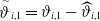 $ {\stackrel{\sim }{\vartheta }}_{i,1}={\vartheta }_{i,1}-{\widehat{\vartheta }}_{i,1}$
, where
 $ {\widehat{\vartheta }}_{i,1}$
is the estimation of
 $ {\vartheta }_{i,1}$
.
In conventional backstepping control, the control signal
 $ {\boldsymbol{\Psi }}_{i}^{c}$
is subject to repeated differentiation, where increasing system order necessitates proportional differentiation operations, thereby inducing the EI phenomenon. To resolve this inherent limitation, we implement a fixed-time command filter (FCF) that
 \begin{align} {{\Delta }}_{\tau }{\dot{\boldsymbol{\Psi }}}_{i}^{d}=\left({\boldsymbol{\Psi }}_{i}^{d}-{\boldsymbol{\Psi }}_{i}^{c}\right){||{\boldsymbol{\Psi }}_{i}^{d}-{\boldsymbol{\Psi }}_{i}^{c}||}^{p-1}+\left({\boldsymbol{\Psi }}_{i}^{d}-{\boldsymbol{\Psi }}_{i}^{c}\right){||{\boldsymbol{\Psi }}_{i}^{d}-{\boldsymbol{\Psi }}_{i}^{c}||}^{q-1},{\boldsymbol{\Psi }}_{i}^{d}\left(0\right)={\boldsymbol{\Psi }}_{i}^{c}\left(0\right)\end{align}
where
 $ {\boldsymbol{\Psi }}_{i}^{d}$
is the output of the FCF and
 $ {\boldsymbol{\Psi }}_{i}^{c}$
is the input;
 $ {{\Delta }}_{\tau }$
stands for a little parameter.
To tackle the impact of filtering error, a compensative strategy is formulated as
 \begin{align} {\boldsymbol{\Upsilon }}_{i,n}={\mathbf{z}}_{i,n}-{\mathbf{w}}_{i,n},n=\mathrm{1, 2},3\end{align}
The first order error compensative signal
 $ {\mathbf{w}}_{i,1}$
is defined as
 \begin{align} {\dot{\mathbf{w}}}_{i,1}=-{\tau }_{i,1}{\mathbf{w}}_{i,1}-{\mu }_{i,1}{\mathbf{w}}_{i,1}{||{\mathbf{w}}_{i,1}||}^{p-1}-{\lambda }_{i,1}{\mathbf{w}}_{i,1}{||{\mathbf{w}}_{i,1}||}^{q-1}+\left({l}_{i}+{d}_{i}\right)\left({\boldsymbol{\Psi }}_{i,1}^{d}-{\boldsymbol{\Psi }}_{i,1}^{c}\right)\end{align}
in which
 $ {\tau }_{i,1}$
,
 $ {\mu }_{i,1}$
,
 $ {\lambda }_{i,1}$
are positive design parameters;
 $ p$
and
 $ q$
represent odd numbers to be designed, satisfying
 $ 0 \lt p \lt 1$
,
 $ q \gt 1$
.
The virtual control signal
 $ {\boldsymbol{\Psi }}_{i,1}^{c}$
of the follower
 $ i$
in the first order subsystem is devised as follows:
 \begin{align} {\boldsymbol{\Psi }}_{i,1}^{c}=\frac{1}{{l}_{i}+{d}_{i}}\left[\begin{array}{l}-{\tau }_{i,1}{\boldsymbol{\Upsilon }}_{i,1}-{\chi }_{i,1}{\boldsymbol{\Upsilon }}_{i,1}{||{\boldsymbol{\Upsilon }}_{i,1}||}^{p-1}-{\lambda }_{i,1}{\boldsymbol{\Upsilon }}_{i,1}{||{\boldsymbol{\Upsilon }}_{i,1}||}^{q-1}\\[4pt] -\dfrac{{\boldsymbol{\Upsilon }}_{i,1}}{2}-\dfrac{{\boldsymbol{\Upsilon }}_{i,1}}{2{\ell}_{i,1}^{2}}{\widehat{\vartheta }}_{i,1}{\mathbf{F}}_{i,1}^{T}{\mathbf{F}}_{i,1}+{l}_{i}{\boldsymbol{\Pi }}_{j,1}+{d}_{i}{\dot{\omega }}_{d}\end{array}\right]\end{align}
where
 $ {\chi }_{i,1}$
and
 $ {\lambda }_{i,1}$
are positive design parameters.
Define the second order subsystem error as
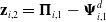 $ {\mathbf{z}}_{i,2}={\boldsymbol{\Pi }}_{i,1}-{\boldsymbol{\Psi }}_{i,1}^{d}$
, Construct the Lyapunov function
 $ {L}_{i,1}=\frac{{\boldsymbol{\Upsilon }}_{i,1}^{T}{\boldsymbol{\Upsilon }}_{i,1}}{2}+\frac{{\mathbf{w}}_{i,1}^{T}{\mathbf{w}}_{i,1}}{2}+\frac{{\stackrel{\sim }{\vartheta }}_{i,1}^{2}}{2{\kappa }_{i,1}}$
, in which
 $ {\kappa }_{i,1}$
represents a positive parameter. According to the derivative of tracking error (18) and compensative strategy (21), we get
 \begin{align} {\dot{L}}_{i,1} {} &={\boldsymbol{\Upsilon }}_{i,1}^{T}{\dot{\boldsymbol{\Upsilon }}}_{i,1}+{\mathbf{w}}_{i,1}^{T}{\dot{\mathbf{w}}}_{i,1}+\frac{{\dot{\stackrel{\sim }{\vartheta }}}_{i,1}{\stackrel{\sim }{\vartheta }}_{i,1}}{{\kappa }_{i,1}}\nonumber\\ {} &=\left({l}_{i}+{d}_{i}\right){\boldsymbol{\Upsilon }}_{i,1}^{T}\left({\boldsymbol{\Pi }}_{i,1}+{\Delta }{\boldsymbol{\Omega }}_{i,1}\right)-{l}_{i}{\boldsymbol{\Upsilon }}_{i,1}^{T}\left({\boldsymbol{\Pi }}_{j,1}+{\Delta }{\boldsymbol{\Omega }}_{j,1}\right)\nonumber\\ {} &\quad-{d}_{i}{\boldsymbol{\Upsilon }}_{i,1}^{T}{\dot{\omega }}_{d}-{\boldsymbol{\Upsilon }}_{i,1}^{T}{\dot{\mathbf{w}}}_{i,1}+{\mathbf{w}}_{i,1}^{T}{\dot{\mathbf{w}}}_{i,1}-\frac{{\dot{\widehat{\vartheta }}}_{i,1}{\stackrel{\sim }{\vartheta }}_{i,1}}{{\kappa }_{i,1}}\end{align}
The RBFNN weight updating law is designed as
 \begin{align} {\dot{\widehat{\vartheta }}}_{i,1}=\frac{{\kappa }_{i,1}{\boldsymbol{\Upsilon }}_{i,1}^{T}{\boldsymbol{\Upsilon }}_{i,1}}{2{\ell}_{i,1}^{2}}{\mathbf{F}}_{i,1}^{T}{\mathbf{F}}_{i,1}-{\xi }_{i,1}{\widehat{\vartheta }}_{i,1}-{\varsigma }_{i,1}{\widehat{\vartheta }}_{i,1}^{p}-{\varpi }_{i,1}{\widehat{\vartheta }}_{i,1}^{q}\end{align}
with
 $ {\xi }_{i,1}$
,
 $ {\varsigma }_{i,1}$
and
 $ {\varpi }_{i,1}$
being parameters to be designed.
According to Young’s inequality and Lemma 2, we get
 \begin{align} \big(({l}_{i}+{d}_{i}){\boldsymbol{\Upsilon }}_{i,1}^{T}{\Delta }{\boldsymbol{\Omega }}_{i,1}-{l}_{i}{\boldsymbol{\Upsilon }}_{i,1}^{T}{\Delta }{\boldsymbol{\Omega }}_{j,1}\big) {} &\le \frac{{\vartheta }_{i,1}{\boldsymbol{\Upsilon }}_{i,1}^{T}{\boldsymbol{\Upsilon }}_{i,1}{\mathbf{F}}_{i,1}^{T}{\mathbf{F}}_{i,1}}{2{\ell}_{i,1}^{2}}+\frac{{\ell}_{i,1}^{2}}{2}+\frac{{||{\boldsymbol{\Upsilon }}_{i,1}||}^{2}}{2}+\frac{{\zeta }_{i,1}^{2}}{2}\nonumber\\ {\stackrel{\sim }{\vartheta }}_{i,1}{\widehat{\vartheta }}_{i,1} {} &\le \frac{{\vartheta }_{i,1}^{2}}{2}-\frac{{\stackrel{\sim }{\vartheta }}_{i,1}^{2}}{2}\nonumber\\ {\stackrel{\sim }{\vartheta }}_{i,1}{\widehat{\vartheta }}_{i,1}^{p} {} &\le \frac{2{\vartheta }_{i,1}^{p+1}}{p+1}-\frac{{\stackrel{\sim }{\vartheta }}_{i,1}^{p+1}}{p+1}\nonumber\\ {\stackrel{\sim }{\vartheta }}_{i,1}{\widehat{\vartheta }}_{i,1}^{q} {} &\le \frac{2{\vartheta }_{i,1}^{q+1}}{q+1}-\frac{{\stackrel{\sim }{\vartheta }}_{i,1}^{q+1}}{q+1} {} \end{align}
Through the synthesis of (22-26), it can be inferred that
 \begin{align} {\dot{L}}_{i,1} {} &\le -{\tau }_{i,1}{||{\boldsymbol{\Upsilon }}_{i,1}||}^{2}-{\chi }_{i,1}{||{\boldsymbol{\Upsilon }}_{i,1}||}^{p+1}-{\lambda }_{i,1}{||{\boldsymbol{\Upsilon }}_{i,1}||}^{q+1}+{\tau }_{i,1}{\boldsymbol{\Upsilon }}_{i,1}^{T}{\mathbf{w}}_{i,1}+{\mu }_{i,1}{\boldsymbol{\Upsilon }}_{i,1}^{T}{\mathbf{w}}_{i,1}{||{\mathbf{w}}_{i,1}||}^{p-1}\nonumber\\ {} &+{\lambda }_{i,1}{\boldsymbol{\Upsilon }}_{i,1}^{T}{\mathbf{w}}_{i,1}{||{\mathbf{w}}_{i,1}||}^{q-1}-{\tau }_{i,1}{||{\mathbf{w}}_{i,1}||}^{2}-{\mu }_{i,1}{||{\mathbf{w}}_{i,1}||}^{p+1}-{\lambda }_{i,1}{||{\mathbf{w}}_{i,1}||}^{q+1}\nonumber\\ {} &+\frac{{{\ell}}_{i,1}^{2}}{2}+\frac{{\zeta }_{i,1}^{2}}{2}+\left({l}_{i}+{d}_{i}\right){\boldsymbol{\Upsilon }}_{i,1}^{T}{\mathbf{z}}_{i,2}+\left({l}_{i}+{d}_{i}\right){\mathbf{w}}_{i,1}^{T}\left({\boldsymbol{\Psi }}_{i,1}^{d}-{\boldsymbol{\Psi }}_{i,1}^{c}\right)\nonumber\\ {} &+\frac{{\xi }_{i,1}}{{\kappa }_{i,1}}\left(\frac{{\vartheta }_{i,1}^{2}}{2}-\frac{{\stackrel{\sim }{\vartheta }}_{i,1}^{2}}{2}\right)+\frac{{\varsigma }_{i,1}}{{\kappa }_{i,1}}\left(\frac{2{\vartheta }_{i,1}^{p+1}}{p+1}-\frac{{\stackrel{\sim }{\vartheta }}_{i,1}^{p+1}}{p+1}\right)+\frac{{\varpi }_{i,1}}{{\kappa }_{i,1}}\left(\frac{2{\vartheta }_{i,1}^{q+1}}{q+1}-\frac{{\stackrel{\sim }{\vartheta }}_{i,1}^{q+1}}{q+1}\right) {} \end{align}
Step 2. According to Step 1, the error in second order subsystem for the follower
 $ i$
can be written as
 \begin{align} {\mathbf{z}}_{i,2}={\boldsymbol{\Pi }}_{i,1}-{\boldsymbol{\Psi }}_{i,1}^{d}\end{align}
The compensative signal
 $ {\mathbf{w}}_{i,2}$
is defined as
 \begin{align} {\dot{\mathbf{w}}}_{i,2}=-{\tau }_{i,2}{\mathbf{w}}_{i,2}-{\mu }_{i,2}{\mathbf{w}}_{i,2}{||{\mathbf{w}}_{i,2}||}^{p-1}-{\lambda }_{i,2}{\mathbf{w}}_{i,2}{||{\mathbf{w}}_{i,2}||}^{q-1}+\frac{\partial {\boldsymbol{\Pi }}_{i,1}}{\partial {\boldsymbol{\Psi }}_{i,2}}{\boldsymbol{\Psi }}_{i,2}^{d}-\frac{\partial {\boldsymbol{\Pi }}_{i,1}}{\partial {\boldsymbol{\Psi }}_{i,2}}{\boldsymbol{\Psi }}_{i,2}^{c}\end{align}
The non-affine item
 $ {\boldsymbol{\Pi }}_{i,1}$
takes partial derivatives of
 $ {\boldsymbol{\Psi }}_{i,1}$
and
 $ {\boldsymbol{\Psi }}_{i,2}$
respectively, we have
 \begin{align} \frac{{\boldsymbol{\Pi }}_{i,1}}{\partial {\boldsymbol{\Psi }}_{i,1}}={0}^{3\times 3}\end{align}
 \begin{align} \frac{\partial {\boldsymbol{\Pi }}_{i,1}}{\partial {\boldsymbol{\Psi }}_{i,2}}=\left[\begin{array}{c@{\quad}c@{\quad}c}\mathrm{cos}{\boldsymbol{\Psi }}_{i,{2}_{\left(2\right)}}\mathrm{cos}{\boldsymbol{\Psi }}_{i,{2}_{\left(3\right)}} & {} {-}{\boldsymbol{\Psi }}_{i,{2}_{\left(1\right)}}\mathrm{sin}{\boldsymbol{\Psi }}_{i,{2}_{\left(2\right)}}\mathrm{cos}{\boldsymbol{\Psi }}_{i,{2}_{\left(3\right)}} & -{\boldsymbol{\Psi }}_{i,{2}_{\left(1\right)}}\mathrm{cos}{\boldsymbol{\Psi }}_{i,{2}_{\left(2\right)}}\mathrm{sin}{\boldsymbol{\Psi }}_{i,{2}_{\left(3\right)}} {} \\ \mathrm{sin}{\boldsymbol{\Psi }}_{i,{2}_{\left(2\right)}} {}& {\boldsymbol{\Psi }}_{i,{2}_{\left(1\right)}}\mathrm{cos}{\boldsymbol{\Psi }}_{i,{2}_{\left(2\right)}} & 0 {} \\ \mathrm{cos}{\boldsymbol{\Psi }}_{i,{2}_{\left(2\right)}}\mathrm{sin}{\boldsymbol{\Psi }}_{i,{2}_{\left(3\right)}} & -{\boldsymbol{\Psi }}_{i,{2}_{\left(1\right)}}\mathrm{sin}{\boldsymbol{\Psi }}_{i,{2}_{\left(2\right)}}\mathrm{sin}{\boldsymbol{\Psi }}_{i,{2}_{\left(3\right)}} & {\boldsymbol{\Psi }}_{i,{2}_{\left(1\right)}}\mathrm{cos}{\boldsymbol{\Psi }}_{i,{2}_{\left(2\right)}}\mathrm{cos}{\boldsymbol{\Psi }}_{i,{2}_{\left(3\right)}} {} \end{array}\right]\end{align}
Introduce the error in third order subsystem as
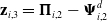 $ {\mathbf{z}}_{i,3}={\boldsymbol{\Pi }}_{i,2}-{\boldsymbol{\Psi }}_{i,2}^{d}$
. Thus, combining dynamics model (15) and compensative strategy (21), we take the derivative of
 $ {\mathbf{z}}_{i,2}$
as
 \begin{align} {\dot{\mathbf{z}}}_{i,2} {} &={\dot{\boldsymbol{\Pi }}}_{i,1}-{\dot{\boldsymbol{\Psi }}}_{i,1}^{d}\nonumber\\ {}&=\frac{\partial {\boldsymbol{\Pi }}_{i,1}}{\partial {\boldsymbol{\Psi }}_{i,1}}{\dot{\boldsymbol{\Psi }}}_{i,1}+\frac{\partial {\boldsymbol{\Pi }}_{i,1}}{\partial {\boldsymbol{\Psi }}_{i,2}}{\dot{\boldsymbol{\Psi }}}_{i,2}-{\dot{\boldsymbol{\Psi }}}_{i,1}^{d}\nonumber\\ {}&=\frac{\partial {\boldsymbol{\Pi }}_{i,1}}{\partial {\boldsymbol{\Psi }}_{i,1}}\left({\boldsymbol{\Pi }}_{i,1}+{\Delta }{\boldsymbol{\Omega }}_{i,1}\right)+\frac{\partial {\boldsymbol{\Pi }}_{i,1}}{\partial {\boldsymbol{\Psi }}_{i,2}}\left({\boldsymbol{\Xi }}_{i}+{\boldsymbol{\Upsilon }}_{i,3}+{\mathbf{w}}_{i,3}+{\boldsymbol{\Psi }}_{i,2}^{d}+{\Delta }{\boldsymbol{\Omega }}_{i,2}\right)-{\dot{\boldsymbol{\Psi }}}_{i,1}^{d} {} \end{align}
Similarly to step 1, define
 $ {\Delta }{{\Omega }}_{2}=||\sum _{k=1}^{2}\,\frac{\partial {\boldsymbol{\Pi }}_{i,1}}{\partial {\boldsymbol{\Psi }}_{i,k}}{\Delta }{\boldsymbol{\Omega }}_{i,k}||$
, the estimation based on RBFNN is written as
 $ {\Delta }{\stackrel{-}{{\Omega }}}_{2}={\boldsymbol{\Theta }}_{i,2}^{T}{\mathbf{F}}_{i,2}+{\epsilon }_{i,2}$
, where
 $ \left|{\epsilon }_{i,2}\right|\le {\zeta }_{i,2}$
. Define
 $ {\vartheta }_{i,2}={||{\Theta }_{i,2}||}^{2}$
, the estimation of
 $ {\vartheta }_{i,2}$
as
 $ {\widehat{\vartheta }}_{i,2}$
, then the estimation error
 $ {\stackrel{\sim }{\vartheta }}_{i,2}$
can be written as
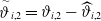 $ {\stackrel{\sim }{\vartheta }}_{i,2}={\vartheta }_{i,2}-{\widehat{\vartheta }}_{i,2}$
.
We devise the virtual control signal
 $ {\boldsymbol{\Psi }}_{i,2}^{c}$
of the follower
 $ i$
in the second order subsystem as
 \begin{align} \begin{array}{l}{\boldsymbol{\Psi }}_{i,2}^{c}={\left(\dfrac{\partial {\boldsymbol{\Pi }}_{i,1}}{\partial {\boldsymbol{\Psi }}_{i,2}}\right)}^{-1}\left(\begin{array}{l}-{\tau }_{,2}{\boldsymbol{\Upsilon }}_{i,2}-{\chi }_{i,2}{\boldsymbol{\Upsilon }}_{i,2}{||{\boldsymbol{\Upsilon }}_{i,2}||}^{p-1}-{\lambda }_{i,2}{\boldsymbol{\Upsilon }}_{i,2}{||{\boldsymbol{\Upsilon }}_{i,2}||}^{q-1}-\frac{{\boldsymbol{\Upsilon }}_{i,2}}{2}\\[6pt] -\dfrac{{}_{i,2}}{2{\ell}_{i,2}^{2}}{\widehat{\vartheta }}_{i,2}{\mathbf{F}}_{i,2}^{T}{\mathbf{F}}_{i,2}-\dfrac{\partial {\boldsymbol{\Pi }}_{i,1}}{\partial {\boldsymbol{\Psi }}_{i,1}}{\boldsymbol{\Pi }}_{i,1}-\dfrac{\partial {\boldsymbol{\Pi }}_{i,1}}{\partial {\boldsymbol{\Psi }}_{i,2}}{\boldsymbol{\Xi }}_{i}+{\dot{\boldsymbol{\Psi }}}_{i,1}^{d}\end{array}\right)\end{array}\end{align}
Let us consider the Lyapunov function as
 $ {L}_{i,2}=\frac{{\boldsymbol{\Upsilon }}_{i,2}^{T}{\boldsymbol{\Upsilon }}_{i,2}}{2}+\frac{{\mathbf{w}}_{i,2}^{T}{\mathbf{w}}_{i,2}}{2}+\frac{{\stackrel{\sim }{\vartheta }}_{i,2}^{2}}{2{\kappa }_{i,2}}$
. By merging (32), we get
 \begin{align} {\dot{L}}_{i,2} {} &={\boldsymbol{\Upsilon }}_{i,2}^{T}{\dot{\boldsymbol{\Upsilon }}}_{i,2}+{\mathbf{w}}_{i,2}^{T}{\dot{\mathbf{w}}}_{i,2}+\frac{{\dot{\stackrel{\sim }{\vartheta }}}_{i,2}{\stackrel{\sim }{\vartheta }}_{i,2}}{{\kappa }_{i,2}}\nonumber\\ {} &={\boldsymbol{\Upsilon }}_{i,2}^{T}\left({\dot{\mathbf{z}}}_{i,2}-{\dot{\mathbf{w}}}_{i,2}\right)+{\mathbf{w}}_{i,2}^{T}{\dot{\mathbf{w}}}_{i,2}+\frac{\left({\dot{\vartheta }}_{i,2}-{\dot{\widehat{\vartheta }}}_{i,2}\right){\stackrel{\sim }{\vartheta }}_{i,2}}{{\kappa }_{i,2}}\nonumber\\ {} &={\boldsymbol{\Upsilon }}_{i,2}^{T}\left(\frac{\partial {\boldsymbol{\Pi }}_{i,1}}{\partial {\boldsymbol{\Psi }}_{i,1}}{\Delta }{\boldsymbol{\Omega }}_{i,1}+\frac{\partial {\boldsymbol{\Pi }}_{i,1}}{\partial {\boldsymbol{\Psi }}_{i,2}}{\Delta }{\boldsymbol{\Omega }}_{i,2}\right)-{\boldsymbol{\Upsilon }}_{i,2}^{T}{\dot{\boldsymbol{\Psi }}}_{i,1}^{d}-{\boldsymbol{\Upsilon }}_{i,2}^{T}{\dot{\mathbf{w}}}_{i,2}+{\mathbf{w}}_{i,2}^{T}{\dot{\mathbf{w}}}_{i,2}-\frac{{\dot{\widehat{\vartheta }}}_{i,2}{\stackrel{\sim }{\vartheta }}_{i,2}}{{\kappa }_{i,2}}\nonumber\\[4pt] {} &\quad+{\boldsymbol{\Upsilon }}_{i,2}^{T}\frac{\partial {\boldsymbol{\Pi }}_{i,1}}{\partial {\boldsymbol{\Psi }}_{i,1}}{\boldsymbol{\Pi }}_{i,1}+{\boldsymbol{\Upsilon }}_{i,2}^{T}\frac{\partial {\boldsymbol{\Pi }}_{i,1}}{\partial {\boldsymbol{\Psi }}_{i,2}}{\boldsymbol{\Xi }}_{i}+{\boldsymbol{\Upsilon }}_{i,2}^{T}\frac{\partial {\boldsymbol{\Pi }}_{i,1}}{\partial {\boldsymbol{\Psi }}_{i,2}}{\boldsymbol{\Upsilon }}_{i,3}+{\boldsymbol{\Upsilon }}_{i,2}^{T}\frac{\partial {\boldsymbol{\Pi }}_{i,1}}{\partial {\boldsymbol{\Psi }}_{i,2}}\left({\mathbf{w}}_{i,3}+{\boldsymbol{\Psi }}_{i,2}^{d}\right)\end{align}
Similarly, the RBFNN weight updating law is designed as
 \begin{align} {\dot{\widehat{\vartheta }}}_{i,2}=\frac{{\kappa }_{i,2}{\boldsymbol{\Upsilon }}_{i,2}^{T}{\boldsymbol{\Upsilon }}_{i,2}}{2{{\ell}}_{i,2}^{2}}{\mathbf{F}}_{i,2}^{T}{\mathbf{F}}_{i,2}-{\xi }_{i,2}{\widehat{\vartheta }}_{i,2}-{\varsigma }_{i,2}{\widehat{\vartheta }}_{i,2}^{p}-{\varpi }_{i,2}{\widehat{\vartheta }}_{i,2}^{q}\end{align}
By applying Lemma 1 and Lemma 2, the inequality (36) is obtained:
 \begin{align} {\boldsymbol{\Upsilon }}_{i,2}\bigg(\frac{\partial {\boldsymbol{\Pi }}_{i,1}}{\partial {\boldsymbol{\Psi }}_{i,1}}{\Delta }{\boldsymbol{\Omega }}_{i,1}+\frac{\partial {\boldsymbol{\Pi }}_{i,1}}{\partial {\boldsymbol{\Psi }}_{i,2}}{\Delta }{\boldsymbol{\Omega }}_{i,2}\!\bigg) {} &\le \frac{{\vartheta }_{i,2}{\boldsymbol{\Upsilon }}_{i,2}^{T}{\boldsymbol{\Upsilon }}_{i,2}{\mathbf{F}}_{i,2}^{T}{\mathbf{F}}_{i,2}}{2{\ell}_{i,2}^{2}}+\frac{{\ell}_{i,2}^{2}}{2}+\frac{{||{\boldsymbol{\Upsilon }}_{i,2}||}^{2}}{2}+\frac{{\zeta }_{i,2}^{2}}{2}\nonumber\\ {\stackrel{\sim }{\vartheta }}_{,2}{\widehat{\vartheta }}_{i,2} {} &\le \frac{{\vartheta }_{i,2}^{2}}{2}-\frac{{\stackrel{\sim }{\vartheta }}_{i,2}^{2}}{2}\nonumber\\ {\stackrel{\sim }{\vartheta }}_{i,2}{\widehat{\vartheta }}_{i,2}^{p} {} &\le \frac{2{\vartheta }_{i,2}^{p+1}}{p+1}-\frac{{\stackrel{\sim }{\vartheta }}_{i,2}^{p+1}}{p+1}\nonumber\\ {\stackrel{\sim }{\vartheta }}_{i,2}{\widehat{\vartheta }}_{i,2}^{q} {} &\le \frac{2{\vartheta }_{i,2}^{q+1}}{q+1}-\frac{{\stackrel{\sim }{\vartheta }}_{i,2}^{q+1}}{q+1} {} \end{align}
By substituting compensative signal (29), virtual control signal (33), RBFNN weight updating law (35) and the inequality (36) into (34), we get
 \begin{align} {\dot{L}}_{i,2} {} &\le -{\tau }_{i,2}{||{\boldsymbol{\Upsilon }}_{i,2}||}^{2}-{\chi }_{i,2}{||{\boldsymbol{\Upsilon }}_{i,2}||}^{p+1}-{\lambda }_{i,2}{||{\boldsymbol{\Upsilon }}_{i,2}||}^{q+1}+{\tau }_{i,2}{\boldsymbol{\Upsilon }}_{i,2}^{T}{\mathbf{w}}_{i,2}+{\mu }_{i,2}{\boldsymbol{\Upsilon }}_{i,2}^{T}{\mathbf{w}}_{i,2}{||{\mathbf{w}}_{i,2}||}^{p-1}\nonumber\\ {} &\quad+{\lambda }_{i,2}{\boldsymbol{\Upsilon }}_{i,2}^{T}{\mathbf{w}}_{i,2}{||{\mathbf{w}}_{i,2}||}^{q-1}-{\tau }_{i,2}{||{\mathbf{w}}_{i,2}||}^{2}-{\mu }_{i,2}{||{\mathbf{w}}_{i,2}||}^{p+1}-{\lambda }_{i,2}{||{\mathbf{w}}_{i,2}||}^{q+1}+\frac{{\ell}_{i,2}^{2}}{2}+\frac{{\zeta }_{i,2}^{2}}{2}\nonumber\\ {} &\quad+{\boldsymbol{\Upsilon }}_{i,2}^{T}\frac{\partial {\boldsymbol{\Pi }}_{i,1}}{\partial {\boldsymbol{\Psi }}_{i,2}}{\boldsymbol{\Upsilon }}_{i,3}+{\mathbf{w}}_{i,2}^{T}\frac{\partial {\boldsymbol{\Pi }}_{i,1}}{\partial {\boldsymbol{\Psi }}_{i,2}}\left({\boldsymbol{\Psi }}_{i,2}^{d}-{\boldsymbol{\Psi }}_{i,2}^{c}\right)\nonumber\\ {} &\quad+\frac{{\xi }_{i,2}}{{\kappa }_{i,2}}\left(\frac{{\vartheta }_{i,2}^{2}}{2}-\frac{{\stackrel{\sim }{\vartheta }}_{i,2}^{2}}{2}\right)+\frac{{\varsigma }_{i,2}}{{\kappa }_{i,2}}\left(\frac{2{\vartheta }_{i,2}^{p+1}}{p+1}-\frac{{\stackrel{\sim }{\vartheta }}_{i,2}^{p+1}}{p+1}\right)+\frac{{\varpi }_{i,2}}{{\kappa }_{i,2}}\left(\frac{2{\vartheta }_{i,2}^{q+1}}{q+1}-\frac{{\stackrel{\sim }{\vartheta }}_{i,2}^{q+1}}{q+1}\right)\end{align}
Step 3. According to Step 2, we express the third-order error for the follower
 $ i$
in terms of
 \begin{align} {\mathbf{z}}_{i,3}={\boldsymbol{\Pi }}_{i,2}-{\boldsymbol{\Psi }}_{i,2}^{d}\end{align}
The compensative signal
 $ {\mathbf{w}}_{i,3}$
is developed as
 \begin{align} {\dot{\mathbf{w}}}_{i,3}=-{\tau }_{i,3}{\mathbf{w}}_{i,3}-{\mu }_{i,3}{\mathbf{w}}_{i,3}{||{\mathbf{w}}_{i,3}||}^{p-1}-{\lambda }_{i,3}{\mathbf{w}}_{i,3}{||{\mathbf{w}}_{i,3}||}^{q-1}\end{align}
Thus, the derivative of
 $ {\mathbf{z}}_{i,3}$
becomes
 \begin{align} {\dot{\mathbf{z}}}_{i,3} {} &={\dot{\boldsymbol{\Pi }}}_{i,2}-{\dot{\boldsymbol{\Psi }}}_{i,2}^{d}\nonumber\\ {} &=\sum _{k=1}^{3}\,\frac{\partial {\boldsymbol{\Pi }}_{i,2}}{\partial {\boldsymbol{\Psi }}_{i,k}}{\dot{\boldsymbol{\Psi }}}_{i,k}-{\dot{\boldsymbol{\Psi }}}_{i,2}^{d}\nonumber\\ {} &=\sum _{k=1}^{2}\,\frac{\partial {\boldsymbol{\Pi }}_{i,2}}{\partial {\boldsymbol{\Psi }}_{i,k}}\left({\boldsymbol{\Pi }}_{i,k}+{\Delta }{\boldsymbol{\Omega }}_{i,k}\right)+\frac{\partial {\boldsymbol{\Pi }}_{i,2}}{\partial {\boldsymbol{\Psi }}_{i,2}}{\boldsymbol{\Xi }}_{i}+\frac{\partial {\boldsymbol{\Pi }}_{i,2}}{\partial {\boldsymbol{\Psi }}_{i,3}}{\mathbf{u}}_{fi}-{\dot{\boldsymbol{\Psi }}}_{i,2}^{d}\end{align}
The non-affine item
 $ {\boldsymbol{\Pi }}_{i,2}$
takes partial derivatives of
 $ {\boldsymbol{\Psi }}_{i,1}$
,
 $ {\boldsymbol{\Psi }}_{i,2}$
and
 $ {\boldsymbol{\Psi }}_{i,3}$
respectively, we have
 \begin{align} \frac{\partial {\boldsymbol{\Pi }}_{i,2}}{\partial {\boldsymbol{\Psi }}_{i,1}}=-\frac{{\boldsymbol{\Pi }}_{i,2}\otimes \left[\begin{array}{lll}1 {} 0 {} 0\end{array}\right]}{{h}_{s}}\end{align}
where
 $ \otimes $
means the Kronecker product.
 \begin{align} \frac{\partial {\boldsymbol{\Pi }}_{i,2}}{\partial {}_{i,2}}=\left[\begin{array}{c@{\quad}c@{\quad}c}\dfrac{{\boldsymbol{\Psi }}_{i,{3}_{\left(1\right)}}{\rho }_{i}{\boldsymbol{\Psi }}_{i,{2}_{\left(1\right)}}{S}_{i}}{{m}_{i}} {}& 0 {}& 0 {} \\[4pt] \dfrac{{\boldsymbol{\Psi }}_{i,{3}_{\left(2\right)}}{\rho }_{i}{S}_{i}}{2{m}_{i}} {}& 0 {} &0 {} \\[4pt] \dfrac{{\boldsymbol{\Psi }}_{i,{3}_{\left(3\right)}}{\rho }_{i}{S}_{i}}{2{m}_{i}\mathrm{cos}{\boldsymbol{\Psi }}_{i,{2}_{\left(2\right)}}} {}& \dfrac{{\boldsymbol{\Psi }}_{i,{3}_{\left(3\right)}}{\rho }_{i}{S}_{i}{\boldsymbol{\Psi }}_{i,{2}_{\left(1\right)}}\mathrm{t}\mathrm{a}\mathrm{n}{\boldsymbol{\Psi }}_{i,{2}_{\left(2\right)}}}{2{m}_{i}\mathrm{cos}{\boldsymbol{\Psi }}_{i,{2}_{\left(2\right)}}} {}& 0 {} \end{array}\right]\end{align}
 \begin{align} \frac{\partial {\boldsymbol{\Pi }}_{i,2}}{\partial {\boldsymbol{\Psi }}_{i,3}}=diag\left(\begin{array}{l}\dfrac{{\rho }_{i}{{\boldsymbol{\Psi }}_{i,2}^{2}}_{{\mathrm{}}_{\left(1\right)}}{S}_{i}}{2{m}_{i}}+{{\mathrm{s}ech}_{}}^{2}\left({{\boldsymbol{\Psi }}_{i,3}}_{{\mathrm{}}_{\left(1\right)}}\right),\dfrac{{\rho }_{i}{{\boldsymbol{\Psi }}_{i,2}}_{{\mathrm{}}_{\left(1\right)}}{S}_{i}}{2{m}_{i}}+{{\mathrm{s}ech}_{}}^{2}\left({{\boldsymbol{\Psi }}_{i,3}}_{{\mathrm{}}_{\left(2\right)}}\right),\\[12pt] \dfrac{{\rho }_{i}{{\boldsymbol{\Psi }}_{i,2}}_{{\mathrm{}}_{\left(1\right)}}{S}_{i}}{2{m}_{i}\mathrm{cos}{{\boldsymbol{\Psi }}_{i,2}}_{{\mathrm{}}_{\left(2\right)}}}+{{\mathrm{s}ech}_{}}^{2}\left({{\boldsymbol{\Psi }}_{i,3}}_{{\mathrm{}}_{\left(3\right)}}\right)\end{array}\right)\end{align}
Similarly, define
 $ {\Delta }{{\Omega }}_{3}=||\sum _{k=1}^{2}\,\frac{\partial {\boldsymbol{\Pi }}_{i,2}}{\partial {\boldsymbol{\Psi }}_{i,k}}{\Delta }{\boldsymbol{\Omega }}_{i,k}||$
, exploit RBFNN to compensate the deviation:
 \begin{align} {\Delta }{\stackrel{-}{{\Omega }}}_{3}={\boldsymbol{\Theta }}_{i,3}^{T}{\mathbf{F}}_{i,3}+{\epsilon }_{i,3}\end{align}
where
 $ {\mathbf{F}}_{i,3}$
is the basis function vector,
 $ {\boldsymbol{\Theta }}_{i,3}^{T}$
is the weight vector,
 $ \left|{\epsilon }_{i,3}\right|\le {\zeta }_{i,3}$
. Define
 $ {\vartheta }_{i,3}={||{\boldsymbol{\Theta }}_{i,3}||}^{2}$
, then the estimation error
 $ {\stackrel{\sim }{\vartheta }}_{i,3}$
can be written as
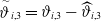 $ {\stackrel{\sim }{\vartheta }}_{i,3}={\vartheta }_{i,3}-{\widehat{\vartheta }}_{i,3}$
, where
 $ {\widehat{\vartheta }}_{i,3}$
is the estimation of
 $ {\vartheta }_{i,3}$
.
We devise the consensus control protocol
 $ {\boldsymbol{\Psi }}_{i,3}^{c}$
of the follower
 $ i$
as
 \begin{align} \begin{array}{l}{\boldsymbol{\Psi }}_{i,3}^{c}={\left(\dfrac{\partial {\boldsymbol{\Pi }}_{i,2}}{\partial {\boldsymbol{\Psi }}_{i,3}}\right)}^{-1}\left(\begin{array}{l}-{\tau }_{i,3}{\boldsymbol{\Upsilon }}_{i,3}-{\chi }_{i,3}{\boldsymbol{\Upsilon }}_{i,3}{||{\boldsymbol{\Upsilon }}_{i,3}||}^{p-1}-{\lambda }_{i,3}{\boldsymbol{\Upsilon }}_{i,3}{||{\boldsymbol{\Upsilon }}_{i,3}||}^{q-1}-\dfrac{{\boldsymbol{\Upsilon }}_{i,3}}{2}\\ -\dfrac{{\boldsymbol{\Upsilon }}_{i,3}}{2{\ell}_{i,j}^{2}}{\widehat{\vartheta }}_{i}{\mathbf{F}}_{i,3}^{T}{\mathbf{F}}_{i,3}-\sum _{k=1}^{2}\,\dfrac{\partial {\boldsymbol{\Pi }}_{i,2}}{\partial {\boldsymbol{\Psi }}_{i,k}}{\boldsymbol{\Pi }}_{i,k}-\dfrac{\partial {\boldsymbol{\Pi }}_{i,2}}{\partial {\boldsymbol{\Psi }}_{i,2}}{\boldsymbol{\Xi }}_{i}+{\dot{\boldsymbol{\Psi }}}_{i,2}^{d}\end{array}\right)\end{array}\end{align}
In terms of the designed real-time continuous control law
 $ {\boldsymbol{\Psi }}_{i,3}^{c}$
causing unnecessary waste of communication resources, a dynamic event-triggered controller is developed as
 \begin{align} {\mathbf{f}}_{i}\left(t\right)={\boldsymbol{\Psi }}_{i,3}^{c}\left(t\right)-\frac{\partial {\boldsymbol{\Pi }}_{i,2}}{\partial {\boldsymbol{\Psi }}_{i,3}}{\boldsymbol{\Upsilon }}_{i,3}{\widehat{\mathit{\eta }}}_{i}^{T}{\widehat{\mathit{\eta }}}_{i}/\sqrt{{\left({\widehat{\mathit{\eta }}}_{i}^{T}\frac{\partial {\boldsymbol{\Pi }}_{i,2}}{\partial {\boldsymbol{\Psi }}_{i,3}}{\boldsymbol{\Upsilon }}_{i,3}\right)}^{2}+{\Lambda }^{2}}\end{align}
Assumption 9.
 $ {\mathit{f}}_{i}\left(t\right)$
is continuously differentiable, and there is a positive upper bound
 $ {\Delta }_{f}$
satisfying
 $ ||{\dot{\mathit{f}}}_{i}\left(t\right)||\le {\Delta }_{f}$
when
 $ t\in \left[{t}_{n},{t}_{n+1}\right)$
.
Considering the specific format of the error variables as
 $ {\mathbf{e}}_{i}\left(t\right)={\mathbf{f}}_{i}\left(t\right)-{\mathbf{u}}_{fi}\left(t\right)$
, define
 $ {\mathbf{e}}_{i}={\left[{e}_{i,1},{e}_{i,2},{e}_{i,3}\right]}^{T}$
, we accessorily design the dynamic event-triggered condition as
 \begin{align} \left\{\begin{array}{llllllllllllllllllll}{\mathbf{u}}_{fi}\left(t\right)={\mathbf{f}}_{i}\left({t}_{n}\right),t\in \left[{t}_{n},{t}_{n+1}\right) {} {} {} {} {} {} {} {} {} {} {} {} {} {} {} {} {} {} {} \\ {t}_{n+1}=\mathrm{i}\mathrm{n}\mathrm{f}\left\{t\in ,\left|{e}_{i,k}\left(t\right)\right|\ge {\wp }_{i,k}\mathrm{t}\mathrm{a}\mathrm{n}\mathrm{h}\left|\frac{{u}_{fi,k}\left(t\right)}{{\hslash }_{i,k}}\right|+{\eta }_{i,k}\left(t\right),k=\mathrm{1, 2},3\right\},\end{array}\right.\end{align}
in which
 $ {\wp }_{i}={\left[{\wp }_{i,1},{\wp }_{i,2},{\wp }_{i,3}\right]}^{T}$
,
 $ {\hslash }_{i}={\left[{\hslash }_{i,1},{\hslash }_{i,2},{\hslash }_{i,3}\right]}^{T}$
, both are positive parameter vectors to be set;
 $ {\widehat{\mathit{\eta }}}_{i}={\wp }_{i}+{\mathit{\eta }}_{i}\left(t\right)$
,
 $ {\mathit{\eta }}_{i}\left(t\right)={\left[{\eta }_{i,1},{\eta }_{i,2},{\eta }_{i,3}\right]}^{T}$
satisfies
 \begin{align} {\dot{\eta }}_{i,k}\left(t\right)=-{\partial }_{i,k}{\eta }_{i,k}\left(t\right)-{B}_{i,k}{\eta }_{i,k}^{p}\left(t\right)-{\aleph }_{i,k}{\eta }_{i,k}^{q}\left(t\right)+{\wp }_{i,k}\mathrm{t}\mathrm{a}\mathrm{n}\mathrm{h}\left|\frac{{u}_{fi,k}\left(t\right)}{{\hslash }_{i,k}}\right|-\left|{e}_{i,k}\left(t\right)\right|\end{align}
In (48),
 $ {\mathit{\eta }}_{i}\left(t\right)$
means a dynamic internal trigger variable with
 $ {\mathit{\eta }}_{i,k}\left(0\right) \gt 0$
;
 $ {\partial }_{i}={\left[{\partial }_{i,1},{\partial }_{i,2},{\partial }_{i,3}\right]}^{T}$
,
 $ {\mathbf{B}}_{i}={\left[{B}_{i,1},{B}_{i,2},{B}_{i,3}\right]}^{T}$
,
 $ {\aleph }_{i}={\left[{\aleph }_{i,1},{\aleph }_{i,2},{\aleph }_{i,3}\right]}^{T}$
, they denote positive design parameter vectors.
Remark 1: On the basis of switching condition (47), it can be delivered when
 $ t\in [0,+{\infty })$
, always satisfy
 $ {\wp }_{i,k}\mathrm{t}\mathrm{a}\mathrm{n}\mathrm{h}\left|\frac{{u}_{fi,k}\left(t\right)}{{\hslash }_{i,k}}\right|-\left|{e}_{i,k}\left(t\right)\right| \gt -{\eta }_{i,k}\left(t\right)$
. Then, (48) can be expressed alternatively as
 $ {\dot{\eta }}_{i,k}\left(t\right) \gt -\left({\partial }_{i,k}+1\right){\eta }_{i,k}\left(t\right)-{B}_{i,k}{\eta }_{i,k}^{p}\left(t\right)-{\aleph }_{i,k}{\eta }_{i,k}^{q}\left(t\right)$
. According to the fixed time theory,
 $ \underset{t\to {T}_{s}}{{\mathrm{l}\mathrm{i}\mathrm{m}}_{}}\mathrm{}{\eta }_{i}=0,\underset{{\eta }_{i}\to {0}^{+}}{{\mathrm{l}\mathrm{i}\mathrm{m}}_{}}\mathrm{}{\dot{\eta }}_{i}=0$
. By utilising switching condition (47), it has
 $ \left|{e}_{i,k}\left(t\right)\right| \lt {\wp }_{i,k}\mathrm{t}\mathrm{a}\mathrm{n}\mathrm{h}\left|\frac{{u}_{fi,k}\left(t\right)}{{\hslash }_{i,k}}\right|+{\eta }_{i,k}\left(t\right) \lt {\wp }_{i,k}+{\eta }_{i,k}\left(t\right)$
when
 $ t\in [{t}_{n},{t}_{n+1})$
. Define
 $ {\mathbf{u}}_{fi}\left(t\right)={\mathbf{f}}_{i}\left(t\right)-{\tau }_{i}\left({\wp }_{i}+{\mathit{\eta }}_{i}\left(t\right)\right)$
, where
 $ {\tau }_{i}=\mathrm{m}\mathrm{a}\mathrm{x}\left\{\frac{{f}_{i,k}\left(t\right)-{u}_{fi,k}\left(t\right)}{{\wp }_{i,k}+{\mathit{\eta }}_{i,k}\left(t\right)}\right\},k=\mathrm{1, 2},3$
is continuous meeting
 $ \left|{\tau }_{i}\right| \lt 1$
. Then, choose the Lyapunov function
 $ {L}_{i,3}=\frac{{\boldsymbol{\Upsilon }}_{i,3}^{T}{\boldsymbol{\Upsilon }}_{i,3}}{2}+\frac{{\mathbf{w}}_{i,3}^{T}{\mathbf{w}}_{i,3}}{2}+\frac{{\stackrel{\sim }{\vartheta }}_{i,3}^{2}}{2{\kappa }_{i,3}}$
, we take the derivative of
 $ {L}_{i,3}$
combining (21) and (40) as
 \begin{align} {\dot{L}}_{i,3} {} &={\boldsymbol{\Upsilon }}_{i,3}^{T}{\dot{\boldsymbol{\Upsilon }}}_{i,3}+{\mathbf{w}}_{i,3}^{T}{\dot{\mathbf{w}}}_{i,3}+\frac{{\dot{\stackrel{\sim }{\vartheta }}}_{i,3}{\stackrel{\sim }{\vartheta }}_{i,3}}{{\kappa }_{i,3}}\nonumber\\ {}& ={\boldsymbol{\Upsilon }}_{i,3}^{T}\left({\dot{\mathbf{z}}}_{i,3}-{\dot{\mathbf{w}}}_{i,3}\right)+{\mathbf{w}}_{i,3}^{T}{\dot{\mathbf{w}}}_{i,3}+\frac{\left({\dot{\vartheta }}_{i,3}-{\dot{\widehat{\vartheta }}}_{i,3}\right){\stackrel{\sim }{\vartheta }}_{i,3}}{{\kappa }_{i,3}}\nonumber\\ {}& ={\boldsymbol{\Upsilon }}_{i,3}^{T}\left(\sum _{k=1}^{2}\,\frac{\partial {\boldsymbol{\Pi }}_{i,2}}{\partial {\boldsymbol{\Psi }}_{i,k}}\left({\boldsymbol{\Pi }}_{i,k}+{\Delta }{\boldsymbol{\Omega }}_{i,k}\right)+\frac{\partial {\boldsymbol{\Pi }}_{i,2}}{\partial {\boldsymbol{\Psi }}_{i,2}}{\boldsymbol{\Xi }}_{i}\right)+{\boldsymbol{\Upsilon }}_{i,3}^{T}\frac{\partial {\boldsymbol{\Pi }}_{i,2}}{\partial {\boldsymbol{\Psi }}_{i,3}}{\boldsymbol{\Psi }}_{i,3}^{c}\nonumber\\ {}&\quad -{\boldsymbol{\Upsilon }}_{i,3}^{T}{\dot{\boldsymbol{\Psi }}}_{i,2}^{d}-{\boldsymbol{\Upsilon}}_{i,3}^{T}{\dot{\mathbf{w}}}_{i,3}+{\mathbf{w}}_{i,3}^{T}{\dot{\mathbf{w}}}_{i,3}-\frac{{\dot{\widehat{\vartheta }}}_{i,3}{\stackrel{\sim }{\vartheta }}_{i,3}}{{\kappa }_{i,3}}\nonumber\\ &\quad +{\boldsymbol{\Upsilon }}_{i,3}^{T}\frac{\partial {\boldsymbol{\Pi }}_{i,2}}{\partial {\boldsymbol{\Psi }}_{i,3}}\left(-{\tau }_{i}\left({\wp }_{i}+{\mathit{\eta }}_{i}\left(t\right)\right)-\frac{\partial {\boldsymbol{\Pi }}_{i,2}}{\partial {\boldsymbol{\Psi }}_{i,3}}{\boldsymbol{\Upsilon }}_{i,3}{\widehat{\mathit{\eta }}}_{i}^{T}{\widehat{\mathit{\eta }}}_{i}/\sqrt{{\left({\widehat{\mathit{\eta }}}_{i}^{T}\frac{\partial {\boldsymbol{\Pi }}_{i,2}}{\partial {\boldsymbol{\Psi }}_{i,3}}{\boldsymbol{\Upsilon }}_{i,3}\right)}^{2}+{\Lambda }^{2}}\right)\end{align}
The RBFNN weight updating law is designed as
 \begin{align} {\dot{\widehat{\vartheta }}}_{i,3}=\frac{{\kappa }_{i,3}{\boldsymbol{\Upsilon }}_{i,3}^{T}{\boldsymbol{\Upsilon }}_{i,3}}{2{\ell}_{i,3}^{2}}{\mathbf{F}}_{i,3}^{T}{\mathbf{F}}_{i,3}-{\xi }_{i,3}{\widehat{\vartheta }}_{i,3}-{\varsigma }_{i,3}{\widehat{\vartheta }}_{i,3}^{p}-{\varpi }_{i,3}{\widehat{\vartheta }}_{i,3}^{q}\end{align}
With the help of Young’s inequality and Lemma 2, we get
 \begin{align} {\boldsymbol{\Upsilon }}_{i,3}^{T}\sum _{k=1}^{2}\,\frac{\partial {\boldsymbol{\Pi }}_{i,2}}{\partial {\boldsymbol{\Psi }}_{i,k}}{\Delta }{\boldsymbol{\Omega }}_{i,k} {} &\le \frac{{\vartheta }_{i,3}{\boldsymbol{\Upsilon }}_{i,3}^{T}{\boldsymbol{\Upsilon }}_{i,3}{\mathbf{F}}_{i,3}^{T}{\mathbf{F}}_{i,3}}{2{\ell}_{i,3}^{2}}+\frac{{\ell}_{i,3}^{2}}{2}+\frac{{||{\boldsymbol{\Upsilon }}_{i,3}||}^{2}}{2}+\frac{{\zeta }_{i,3}^{2}}{2}\nonumber\\ {\stackrel{\sim }{\vartheta }}_{i,3}{\widehat{\vartheta }}_{i,3} {} &\le \frac{{\vartheta }_{i,3}^{2}}{2}-\frac{{\stackrel{\sim }{\vartheta }}_{i,3}^{2}}{2}\nonumber\\ {\stackrel{\sim }{\vartheta }}_{i,3}{\widehat{\vartheta }}_{i,3}^{p} {} &\le \frac{2{\vartheta }_{i,3}^{p+1}}{p+1}-\frac{{\stackrel{\sim }{\vartheta }}_{i,3}^{p+1}}{p+1}\nonumber\\ {\stackrel{\sim }{\vartheta }}_{i,3}{\widehat{\vartheta }}_{i,3}^{q} {} &\le \frac{2{\vartheta }_{i,3}^{q+1}}{q+1}-\frac{{\stackrel{\sim }{\vartheta }}_{i,3}^{q+1}}{q+1}\end{align}
Obviously,
 $ -{\tau }_{i}\left({\wp }_{i}+{\mathit{\eta }}_{i}\left(t\right)\right)=-{\tau }_{i}{\widehat{\mathit{\eta }}}_{i}$
. Based on Lemma 4 and Lemma 5, one obtains
 \begin{align} {\boldsymbol{\Upsilon }}_{i,3}^{T}&\frac{\partial {\boldsymbol{\Pi }}_{i,2}}{\partial {\boldsymbol{\Psi }}_{i,3}}\left(-{\tau }_{i}\left({\wp }_{i}+{\mathit{\eta }}_{i}\left(t\right)\right)-\frac{\partial {\boldsymbol{\Pi }}_{i,2}}{\partial {\boldsymbol{\Psi }}_{i,3}}{\boldsymbol{\Upsilon }}_{i,3}{\widehat{\mathit{\eta }}}_{i}^{T}{\widehat{\mathit{\eta }}}_{i}/\sqrt{{\left({\widehat{\mathit{\eta }}}_{i}^{T}\frac{\partial {\boldsymbol{\Pi }}_{i,2}}{\partial {\boldsymbol{\Psi }}_{i,3}}{\boldsymbol{\Upsilon }}_{i,3}\right)}^{2}+{\Lambda }^{2}}\right)\nonumber\\ &\le {\boldsymbol{\Upsilon }}_{i,3}^{T}\frac{\partial {\boldsymbol{\Pi }}_{i,2}}{\partial {\boldsymbol{\Psi }}_{i,3}}{\left[\left|{\widehat{\eta }}_{i,1}\right|,\left|{\widehat{\eta }}_{i,2}\right|,\left|{\widehat{\eta }}_{i,3}\right|\right]}^{T}-{\boldsymbol{\Upsilon }}_{i,3}^{T}\frac{\partial {\boldsymbol{\Pi }}_{i,2}}{\partial {\boldsymbol{\Psi }}_{i,3}}{\boldsymbol{\Upsilon }}_{i,3}{\widehat{\mathit{\eta }}}_{i}^{T}{\widehat{\mathit{\eta }}}_{i}/\sqrt{{\left({\widehat{\mathit{\eta }}}_{i}^{T}\frac{\partial {\boldsymbol{\Pi }}_{i,2}}{\partial {\boldsymbol{\Psi }}_{i,3}}{\boldsymbol{\Upsilon }}_{i,3}\right)}^{2}+{\Lambda }^{2}}\nonumber\\ &\le {\Lambda }\end{align}
Substituting Equations (39), (45) and (50-52) into Equation (49) yields
 \begin{align} {\dot{L}}_{i,3} {} &\le -{\tau }_{i,3}{||{\boldsymbol{\Upsilon }}_{i,3}||}^{2}-{\chi }_{i,1}{||{\boldsymbol{\Upsilon }}_{i,3}||}^{p+1}-{\lambda }_{i,1}{||{\boldsymbol{\Upsilon }}_{i,3}||}^{q+1}+{\tau }_{i,3}{\boldsymbol{\Upsilon }}_{i,3}^{T}{\mathbf{w}}_{i,3}+{\mu }_{i,3}{\boldsymbol{\Upsilon }}_{i,3}^{T}{\mathbf{w}}_{i,3}{||{\mathbf{w}}_{i,3}||}^{p-1}\nonumber\\ {} &+{\lambda }_{i,3}{\boldsymbol{\Upsilon }}_{i,3}^{T}{\mathbf{w}}_{i,3}{||{\mathbf{w}}_{i,3}||}^{q-1}-{\tau }_{i,3}{||{\mathbf{w}}_{i,3}||}^{2}-{\mu }_{i,3}{||{\mathbf{w}}_{i,3}||}^{p+1}-{\lambda }_{i,3}{||{\mathbf{w}}_{i,3}||}^{q+1}+{\Lambda }+\frac{{\ell}_{i,3}^{2}}{2}+\frac{{\zeta }_{,3}^{2}}{2}\nonumber\\ {} &+\frac{{\xi }_{i,3}}{{\kappa }_{i,3}}\left(\frac{{\vartheta }_{i,3}^{2}}{2}-\frac{{\stackrel{\sim }{\vartheta }}_{i,3}^{2}}{2}\right)+\frac{{\varsigma }_{i,3}}{{\kappa }_{i,3}}\left(\frac{2{\vartheta }_{i,3}^{p+1}}{1+p}-\frac{{\stackrel{\sim }{\vartheta }}_{i,3}^{p+1}}{1+p}\right)+\frac{{\varpi }_{i,3}}{{\kappa }_{i,3}}\left(\frac{2{\vartheta }_{i,3}^{q+1}}{1+q}-\frac{{\stackrel{\sim }{\vartheta }}_{i,3}^{q+1}}{1+q}\right)\end{align}
3.3 Stability and feasibility analysis
Theorem 1.
For the nonlinear GHGVs system containing one leader and K followers described in (3) subjected to multisource mismatched uncertainties
 $ \Delta {\mathit{\Omega }}_{i,1}$
and
 $ \Delta {\mathit{\Omega }}_{i,2}$
, under Assumptions 1–8, Lemmas 1–6 and Definitions 1–2, if there exist virtual control signals (23), (33), (45), error compensative signals (22), (29), (39), RBFNN weight updating laws (25), (35), (50) and DETM (46), (47), the semi-global practical stability of the closed loop system can be guaranteed and the output tracking error of followers exponentially converge to a small neighbourhood within a fixed-time
 $ {T}_{s}$
.
Proof. Firstly, based on Equations (27), (37) and (53), we build the Lyapunov function as
 \begin{align} {L}_{i}=\sum _{k=1}^{3}\,{L}_{i,k}=\sum _{k=1}^{3}\,\frac{{\boldsymbol{\Upsilon }}_{i,k}^{T}{\boldsymbol{\Upsilon }}_{i,k}}{2}+\frac{{\mathbf{w}}_{i,k}^{T}{\mathbf{w}}_{i,k}}{2}+\frac{{\stackrel{\sim }{\vartheta }}_{i,k}^{2}}{2{\kappa }_{i,k}}\end{align}
Combined with the above analysis, we have
 \begin{align} \begin{array}{c@{\quad}c}{\dot{L}}_{i} {} \le \sum _{k=1}^{3}\,\left(\begin{array}{c}-{\tau }_{i,k}{||{\boldsymbol{\Upsilon }}_{i,k}||}^{2}-{\chi }_{i,k}{||{\boldsymbol{\Upsilon }}_{i,k}||}^{p+1}-{\lambda }_{i,k}{||{\boldsymbol{\Upsilon }}_{i,k}||}^{q+1}+{\tau }_{i,k}{\boldsymbol{\Upsilon }}_{i,k}^{T}{\mathbf{w}}_{i,k}\\[6pt] +{\mu }_{i,k}{\boldsymbol{\Upsilon }}_{i,k}^{T}{\mathbf{w}}_{i,k}{||{\mathbf{w}}_{i,k}||}^{p-1}+{}_{i,k}{\boldsymbol{\Upsilon }}_{i,k}^{T}{\mathbf{w}}_{i,k}{||{\mathbf{w}}_{i,k}||}^{q-1}+\dfrac{{\ell}_{i,k}^{2}}{2}+\dfrac{{\zeta }_{i,k}^{2}}{2}\\[6pt] -{\tau }_{i,k}{||{\mathbf{w}}_{i,k}||}^{2}-{\mu }_{i,k}{||{\mathbf{w}}_{i,k}||}^{p+1}-{\lambda }_{i,k}{||{\mathbf{w}}_{i,k}||}^{q+1}\\[6pt] +\dfrac{{\xi }_{i,k}}{{\kappa }_{i,k}}\left(\dfrac{{\vartheta }_{i,k}^{2}}{2}-\dfrac{{\stackrel{\sim }{\vartheta }}_{i,k}^{2}}{2}\right)+\dfrac{{\varsigma }_{i,k}}{{\kappa }_{i,k}}\left(\dfrac{2{\vartheta }_{i,k}^{p+1}}{p+1}-\dfrac{{\stackrel{\sim }{\vartheta }}_{i,k}^{p+1}}{p+1}\right)+\dfrac{{\varpi }_{i,k}}{{\kappa }_{i,k}}\left(\dfrac{2{\vartheta }_{i,k}^{q+1}}{q+1}-\dfrac{{\stackrel{\sim }{\vartheta }}_{i,k}^{q+1}}{q+1}\right)\end{array}\right)\\[50pt] {} +\left({l}_{i}+{d}_{i}\right){\boldsymbol{\Upsilon }}_{i,1}^{T}{\mathbf{z}}_{i,2}+\left({l}_{i}+{d}_{i}\right){\mathbf{w}}_{i,1}^{T}\left({\boldsymbol{\Psi }}_{i,1}^{d}-{\boldsymbol{\Psi }}_{i,1}^{c}\right)\\[12pt] {} +{\boldsymbol{\Upsilon }}_{i,2}^{T}\dfrac{\partial {\boldsymbol{\Pi }}_{i,1}}{\partial {\boldsymbol{\Psi }}_{i,2}}{\boldsymbol{\Upsilon }}_{i,3}+{\mathbf{w}}_{i,2}^{T}\dfrac{\partial {\boldsymbol{\Pi }}_{i,1}}{\partial {\boldsymbol{\Psi }}_{i,2}}\left({\boldsymbol{\Psi }}_{i,2}^{d}-{\boldsymbol{\Psi }}_{i,2}^{c}\right)+{\Lambda }\end{array}\end{align}
From Lemma 1, it can be derived
 $ {\boldsymbol{\Upsilon }}_{i,k}^{T}{\mathbf{w}}_{i,k}\le \frac{{||{\mathbf{w}}_{i,k}||}^{2}}{2}+\frac{{||{\boldsymbol{\Upsilon }}_{i,k}||}^{2}}{2}$
,
 $ {\boldsymbol{\Upsilon }}_{i,k}^{T}{\mathbf{w}}_{i,k}{||{\mathbf{w}}_{i,k}||}^{p-1}\le \frac{{||{\boldsymbol{\Upsilon }}_{i,k}||}^{p+1}}{p+1}+\frac{p{||{\mathbf{w}}_{i,k}||}^{p+1}}{p+1}$
,
 $ {\boldsymbol{\Upsilon }}_{i,k}^{T}{\mathbf{w}}_{i,k}{||{\mathbf{w}}_{i,k}||}^{q-1}\le \frac{{||{\boldsymbol{\Upsilon }}_{i,k}||}^{q+1}}{q+1}+\frac{q{||{\mathbf{w}}_{i,k}||}^{q+1}}{q+1}$
,
 $ {\boldsymbol{\Upsilon }}_{i,1}^{T}{\mathbf{z}}_{i,2}\le \left({||{\boldsymbol{\Upsilon }}_{i,1}||}^{2}+\frac{{||{\boldsymbol{\Upsilon }}_{i,2}||}^{2}}{2}+\frac{{||{\mathbf{w}}_{i,1}||}^{2}}{2}\right)$
,
 $ {\boldsymbol{\Upsilon }}_{i,2}^{T}\frac{\partial {\boldsymbol{\Pi }}_{i,1}}{\partial {\boldsymbol{\Psi }}_{i,2}}{\boldsymbol{\Upsilon }}_{i,3}\le \stackrel{-}{\Pi }\frac{{||{\boldsymbol{\Upsilon }}_{i,2}||}^{2}+{||{\boldsymbol{\Upsilon }}_{i,3}||}^{2}}{2}$
. Define
 $ ||{\boldsymbol{\Psi }}_{i,k}^{d}-{\boldsymbol{\Psi }}_{i,k}^{c}||\le {\iota }_{i,k}$
, where
 $ k=\mathrm{1, 2}$
. Then it obtains
 $ {\mathbf{w}}_{i,1}^{T}\left({\boldsymbol{\Psi }}_{i,1}^{d}-{\boldsymbol{\Psi }}_{i,1}^{c}\right)\le \frac{{||{\mathbf{w}}_{i,1}||}^{2}+{\iota }_{i,1}^{2}}{2}$
,
 $ {\mathbf{w}}_{i,2}^{T}\frac{\partial {\boldsymbol{\Pi }}_{i,1}}{\partial {\boldsymbol{\Psi }}_{i,2}}\left({\boldsymbol{\Psi }}_{i,2}^{d}-{\boldsymbol{\Psi }}_{i,2}^{c}\right)\le \stackrel{-}{\Pi }\frac{{||{\mathbf{w}}_{i,2}||}^{2}+{\iota }_{i,2}^{2}}{2}$
.
Finally, Equation (55) is further simplified as
 \begin{align} {\dot{L}}_{i} {} &\le -\sum _{k=1}^{3}\,\frac{{\tau }_{i,k}}{2}{||{\boldsymbol{\Upsilon }}_{i,k}||}^{2}-\sum _{k=1}^{3}\,\left({\chi }_{i,k}-\frac{{\mu }_{i,k}}{p+1}\right){\left({||{\boldsymbol{\Upsilon }}_{i,k}||}^{2}\right)}^{\frac{p+1}{2}}-\sum _{k=1}^{3}\,\left({\lambda }_{i,k}-\frac{{\lambda }_{i,k}}{q+1}\right){\left({||{\boldsymbol{\Upsilon }}_{i,k}||}^{2}\right)}^{\frac{q+1}{2}}\nonumber\\ {} &-\sum _{k=1}^{3}\,\frac{{\tau }_{i,k}}{2}{||{\mathbf{w}}_{i,k}||}^{2}-\sum _{k=1}^{3}\,\frac{{\mu }_{i,k}}{p+1}{\left({||{\mathbf{w}}_{i,k}||}^{2}\right)}^{\frac{p+1}{2}}-\sum _{k=1}^{3}\,\frac{{\lambda }_{i,k}}{q+1}{\left({||{\mathbf{w}}_{i,k}||}^{2}\right)}^{\frac{q+1}{2}}\nonumber\\ {} &-\sum _{k=1}^{3}\,{\xi }_{i,k}\frac{{\stackrel{\sim }{\vartheta }}_{i,k}^{2}}{2{\kappa }_{i,k}}-\sum _{k=1}^{3}\,\frac{{\varsigma }_{i,k}}{p+1}\frac{{2}^{\frac{p+1}{2}}}{{\kappa }_{i,k}^{\frac{1-p}{2}}}{\left(\frac{{\stackrel{\sim }{\vartheta }}_{i,k}^{2}}{2{\kappa }_{i,k}}\right)}^{\frac{p+1}{2}}-\sum _{k=1}^{3}\,\frac{{\varpi }_{i,k}}{q+1}\frac{{2}^{\frac{q+1}{2}}}{{\kappa }_{i,k}^{\frac{1-q}{2}}}{\left(\frac{{\stackrel{\sim }{\vartheta }}_{i,k}^{2}}{2{\kappa }_{i,k}}\right)}^{\frac{q+1}{2}}\nonumber\\ {} &+\sum _{k=1}^{3}\,\left(\frac{{\ell}_{i,k}^{2}}{2}+\frac{{\zeta }_{i,k}^{2}}{2}+\frac{{\xi }_{i,k}}{{\kappa }_{i,k}}\frac{{\vartheta }_{i,k}^{2}}{2}+\frac{{\varsigma }_{i,k}}{{\kappa }_{i,k}}\frac{2{\vartheta }_{i,k}^{p+1}}{p+1}+\frac{{\varpi }_{i,k}}{{\kappa }_{i,k}}\frac{2{\vartheta }_{i,k}^{q+1}}{q+1}\right)\nonumber\\ {}&+\left({l}_{i}+{d}_{i}\right)\left({||{\boldsymbol{\Upsilon }}_{i,1}||}^{2}+{||{\mathbf{w}}_{i,1}||}^{2}+\frac{{||{\boldsymbol{\Upsilon }}_{i,2}||}^{2}+{\iota }_{i,1}^{2}}{2}\right)\nonumber\\ {}&+\stackrel{-}{\Pi }\frac{{||{\boldsymbol{\Upsilon }}_{i,2}||}^{2}+{||{\boldsymbol{\Upsilon }}_{i,3}||}^{2}+{||{\mathbf{w}}_{i,2}||}^{2}+{\iota }_{i,2}^{2}}{2}+{\Lambda }\end{align}
By defining
 \begin{align} {\Gamma }_{i,1} {} &=\mathrm{m}\mathrm{i}\mathrm{n}\left\{\frac{{\tau }_{i,k}}{2}\right\},{\Gamma }_{i,2}=\mathrm{m}\mathrm{i}\mathrm{n}\left\{{\chi }_{i,k}-\frac{{\mu }_{i,k}}{p+1}\right\},{\Gamma }_{i,3}=\mathrm{m}\mathrm{i}\mathrm{n}\left\{{\lambda }_{i,k}-\frac{{\lambda }_{i,k}}{q+1}\right\}\nonumber\\ {\Gamma }_{i,4} {} &=\mathrm{m}\mathrm{i}\mathrm{n}\left\{\frac{{\mu }_{i,k}}{p+1}\right\},{\Gamma }_{i,5}=\mathrm{m}\mathrm{i}\mathrm{n}\left\{\frac{{\lambda }_{i,k}}{q+1}\right\},{\Gamma }_{i,6}=\mathrm{m}\mathrm{i}\mathrm{n}\left\{{\xi }_{i,k}\right\}\nonumber\\ {\Gamma }_{i,7} {} &=\frac{{2}^{\frac{p+1}{2}}}{p+1}\mathrm{m}\mathrm{i}\mathrm{n}\left\{\frac{{\varsigma }_{i,k}}{{\kappa }_{i,k}^{\frac{1-p}{2}}}\right\},{\Gamma }_{i,8}=\frac{{2}^{\frac{q+1}{2}}}{q+1}\mathrm{m}\mathrm{i}\mathrm{n}\left\{\frac{{\varpi }_{i,k}}{{\kappa }_{i,k}^{\frac{1-q}{2}}}\right\} \end{align}
 \begin{align} {\Gamma }_{i,9} {} &=\sum _{k=1}^{3}\,\left(\frac{{\ell}_{i,k}^{2}}{2}+\frac{{\zeta }_{i,k}^{2}}{2}+\frac{{\xi }_{i,k}}{{\kappa }_{i,k}}\frac{{\vartheta }_{i,k}^{2}}{2}+\frac{{\varsigma }_{i,k}}{{\kappa }_{i,k}}\frac{2{\vartheta }_{i,k}^{p+1}}{p+1}+\frac{{\varpi }_{i,k}}{{\kappa }_{i,k}}\frac{2{\vartheta }_{i,}^{q+1}}{q+1}\right)\nonumber\\ {} &\quad+\left({l}_{i}+{d}_{i}\right)\left({||{\boldsymbol{\Upsilon }}_{i,1}||}^{2}+{||{\mathbf{w}}_{i,1}||}^{2}+\frac{{||{\boldsymbol{\Upsilon }}_{i,2}||}^{2}+{\iota }_{i,1}^{2}}{2}\right)\nonumber\\ {} &\quad+\stackrel{-}{\Pi }\frac{{||{\boldsymbol{\Upsilon }}_{i,2}||}^{2}+{||{\boldsymbol{\Upsilon }}_{i,3}||}^{2}+{||{\mathbf{w}}_{i,2}||}^{2}+{\iota }_{i,2}^{2}}{2}+{\Lambda }\end{align}
we get
 \begin{align} {\dot{L}}_{i} {} \le &-{\Gamma }_{i,1}\sum _{k=1}^{3}\,{||{\boldsymbol{\Upsilon }}_{i,k}||}^{2}-{\Gamma }_{,2}\sum _{k=1}^{3}\,{\left({||{\boldsymbol{\Upsilon }}_{i,k}||}^{2}\right)}^{\frac{p+1}{2}}-{\Gamma }_{i,3}\sum _{k=1}^{3}\,{\left({||{\boldsymbol{\Upsilon }}_{i,k}||}^{2}\right)}^{\frac{q+1}{2}}\nonumber\\ {} &-{\Gamma }_{i,1}\sum _{k=1}^{3}\,{||{\mathbf{w}}_{i,k}||}^{2}-{\Gamma }_{i,4}\sum _{k=1}^{3}\,{\left({||{\mathbf{w}}_{i,k}||}^{2}\right)}^{\frac{p+1}{2}}-{\Gamma }_{i,5}\sum _{k=1}^{3}\,{\left({||{\mathbf{w}}_{i,k}||}^{2}\right)}^{\frac{q+1}{2}}\nonumber\\ {} &-{\Gamma }_{i,6}\sum _{k=1}^{3}\,\frac{{\stackrel{\sim }{\vartheta }}_{i,k}^{2}}{2{\kappa }_{i,k}}-{\Gamma }_{i,7}\sum _{k=1}^{3}\,{\left(\frac{{\stackrel{\sim }{\vartheta }}_{i,k}^{2}}{2{\kappa }_{i,k}}\right)}^{\frac{p+1}{2}}-{\Gamma }_{i,8}\sum _{k=1}^{3}\,{\left(\frac{{\stackrel{\sim }{\vartheta }}_{i,k}^{2}}{2{\kappa }_{i,k}}\right)}^{\frac{q+1}{2}}+{\Gamma }_{i,9}\end{align}
Herein, we introduce
 $ L=\sum _{i=1}^{K}\,{L}_{i}$
, it can be obtained that
 \begin{align} \dot{L}\le -{c}_{1}L-{c}_{2}{L}^{\frac{p+1}{2}}-{c}_{3}{L}^{\frac{q+1}{2}}+{\delta }_{a}\end{align}
with
 $ {c}_{1}=\mathrm{m}\mathrm{i}\mathrm{n}\left\{{\Gamma }_{i,1},{\Gamma }_{i,6}\right\}$
,
 $ {c}_{2}=\mathrm{m}\mathrm{i}\mathrm{n}\left\{{\Gamma }_{i,2},{\Gamma }_{i,4},{\Gamma }_{i,7}\right\}$
,
 $ {c}_{3}=\mathrm{m}\mathrm{i}\mathrm{n}\left\{{\Gamma }_{i,3},{\Gamma }_{i,5},{\Gamma }_{i,8}\right\}$
,
 $ {\delta }_{a}=\sum _{i=1}^{K}\,{\Gamma }_{i,9}$
.
Therefore, all signals of GHGVs system (3) are SPFTS on the basis of Lemma 6. An upper bound on the convergence time is given by the following form:
 \begin{align} {T}_{s}\le \mathrm{m}\mathrm{a}\mathrm{x}\left\{\frac{2}{{c}_{2}{{\Delta }}_{\epsilon }(1-p)}\right\}+\mathrm{m}\mathrm{a}\mathrm{x}\left\{\frac{2}{{c}_{1}{{\Delta }}_{\epsilon }(q-1)}\right\}\end{align}
Additionally, by using Lemma 6 we obtain the tracking error vector
 $ {\mathbf{z}}_{i,1}$
is bounded satisfying
 \begin{align} ||{\mathbf{z}}_{i,1}||\le \mathrm{m}\mathrm{i}\mathrm{n}\left\{\frac{{\delta }_{a}}{\left(1-{{\Delta }}_{\epsilon }\right){c}_{1}}{\left(\frac{{\delta }_{a}}{\left(1-{{\Delta }}_{\epsilon }\right){c}_{2}}\right)}^{\frac{2}{p+1}}{\left(\frac{{\delta }_{a}}{\left(1-{{\Delta }}_{\epsilon }\right){c}_{3}}\right)}^{\frac{2}{q+1}}\right\}\end{align}
Proof completed.
Theorem 2
Consider the GHGVs described in (3), we have a fixed positive lower bound
 $ {T}_{p}^{i}$
that drives the event time interval
 $ {T}_{n}^{i}={t}_{n+1}-{t}_{n}$
meeting
 $ {T}_{n}^{i}\ge {T}_{p} \gt 0$
based on the DETM (46),(47), where
 $ {T}_{p}=min\{{T}_{p}^{1},\dots ,{T}_{p}^{K}\}$
. Then Zeno behaviour is prevented.
Proof. Based on the DETM (46), (47) and Assumption 9, we get the following inequality in the interval
 $ \left[{t}_{n},{t}_{n+1}\right)$
:
 \begin{align} \frac{d\left|{e}_{i,k}\left(t\right)\right|}{dt}=\left|{\dot{f}}_{i,k}\left(t\right)-{\dot{u}}_{fi,k}\left(t\right)\right|=\left|{\dot{f}}_{i,k}\left(t\right)-{\dot{f}}_{i,k}\left({t}_{n}\right)\right|=\left|{\dot{f}}_{i,k}\left(t\right)\right| \lt {{\Delta }}_{f}\end{align}
with
 $ {{\Delta }}_{f} \gt 0$
. It is known that
 $ \left|{e}_{i,k}\left({t}_{n}\right)\right|=0$
,
 $ \left|{e}_{i,k}\left(t\right)\right|\le {\int }_{{t}_{n}}^{t}\,{{\Delta }}_{f}dt$
, which means
 $ \left|{e}_{i,k}\left(t\right)\right|\le \left(t-{t}_{n}\right){{\Delta }}_{f}$
. Ulteriorly, when the event trigger condition
 $ \left|{e}_{i,k}\left(t\right)\right|\ge {\wp }_{i,k}\mathrm{t}\mathrm{a}\mathrm{n}\mathrm{h}\left|\frac{{u}_{fi,k}\left(t\right)}{{\hslash }_{i,k}}\right|+{\eta }_{i,k}\left(t\right)$
is destroyed, the control signal will be updated. It means that
 $ \underset{t\to {t}_{n+1}}{{\mathrm{l}\mathrm{i}\mathrm{m}}_{}}\mathrm{}\left|{e}_{i,k}\left(t\right)\right|={\wp }_{i,k}\mathrm{t}\mathrm{a}\mathrm{n}\mathrm{h}\left|\frac{{u}_{fi,k}\left(t\right)}{{\hslash }_{i,k}}\right|+{\eta }_{i,k}\left(t\right)$
. According to Equation (62), it gets
 \begin{align} {T}_{n}^{i}\ge \frac{{\wp }_{i,k}\mathrm{t}\mathrm{a}\mathrm{n}\mathrm{h}\left|{u}_{fi,k}\left(t\right)/{\hslash }_{i,k}\right|+{\eta }_{i,k}\left(t\right)}{{{\Delta }}_{f}}\end{align}
Therefore, for
 $ {T}_{p}^{i} \gt 0$
, there exists
 $ {T}_{p}=\mathrm{m}\mathrm{i}\mathrm{n}\{{T}_{p}^{1},\dots ,{T}_{p}^{K}\}$
that satisfies
 $ {T}_{n}^{i}\ge {T}_{p} \gt 0$
, where
 $ i=\mathrm{1, 2},\cdots ,K$
. Then Zeno behaviour can be avoided. Proof completed.
4.0 Simulations
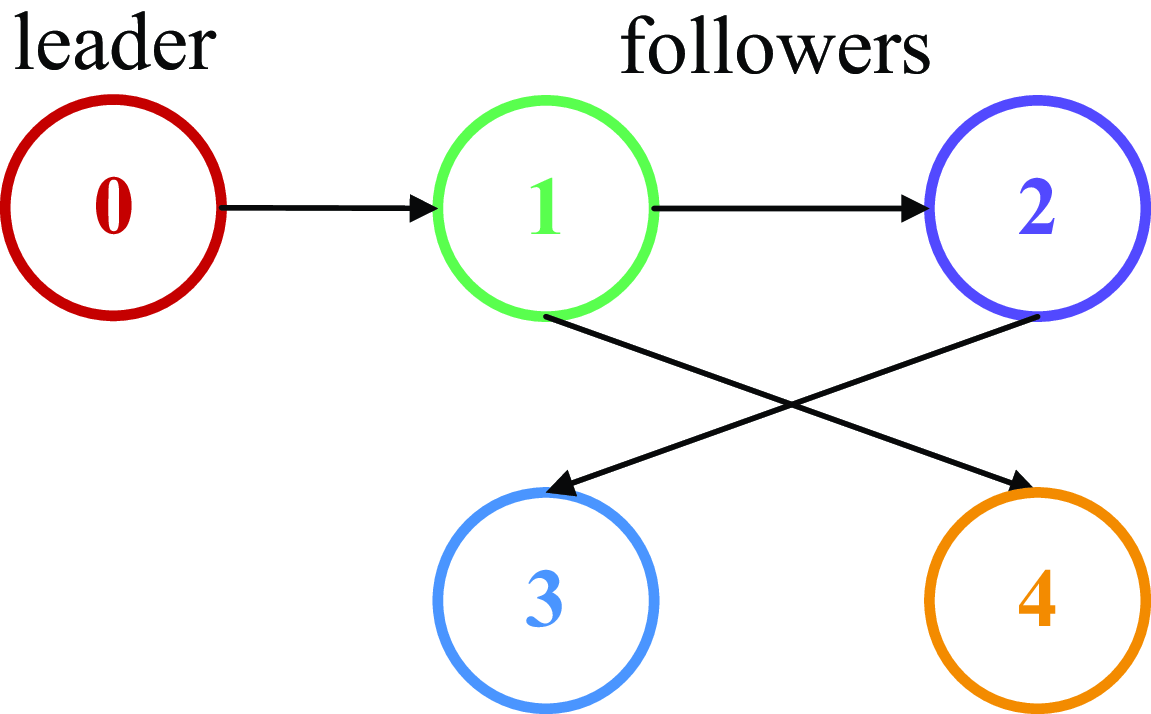
In this work, we use GHGVs system consisting of one leader and four followers to help demonstrate the validity and superiority of the developed distributed consensus strategies.
4.1 Effectiveness verification
To validate the efficacy of the formation control strategy developed in this study, two experimental cases were implemented under identical operational conditions, differentiated solely by their distinct initial state configurations.
Initial conditions of the HGVs in Example 1

Example 1. Assume that the leader HGV is designed to equilibrium glide to increase range. The initial flight conditions of the leader and followers are shown in Table 1.
The uncertainty is chosen as
 $ {\Delta }{\boldsymbol{\Omega }}_{i,1}={\left[3.8\times 1{0}^{-5}{\boldsymbol{\Psi }}_{i,{1}_{\left(1\right)}},1.5\times 1{0}^{-4}{\boldsymbol{\Psi }}_{i,{1}_{\left(2\right)}},4.6\times 1{0}^{-3}{\boldsymbol{\Psi }}_{i,{1}_{\left(3\right)}}\right]}^{T}$
,
 $ {\Delta }{\boldsymbol{\Omega }}_{i,2}={\left[2.5\times 1{0}^{-3}{\boldsymbol{\Psi }}_{i,{2}_{\left(1\right)}},0.8\times 1{0}^{-4}{\boldsymbol{\Psi }}_{i,{2}_{\left(2\right)}},7\times 1{0}^{-3}{\boldsymbol{\Psi }}_{i,{2}_{\left(3\right)}}\right]}^{T}$
.
The gains in the virtual control signals are set as
 $ {\tau }_{i,1}={\chi }_{i,1}={\lambda }_{i,1}=0.03,i=\mathrm{1,3},4$
;
 $ {\tau }_{\mathrm{2,1}}={\chi }_{\mathrm{2,1}}={\lambda }_{\mathrm{2,1}}=0.06$
;
 $ {\tau }_{i,2}={\chi }_{i,2}={\lambda }_{i,2}=0.05$
,
 $ {\tau }_{i,3}={\chi }_{i,3}={\lambda }_{i,3}=0.08$
,
 $ i=\mathrm{1, 2},\mathrm{3, 4}$
;
 $ p=7/9\mathrm{}\mathrm{}$
,
 $ q=9/7\mathrm{}\mathrm{}$
; Choose the design parameters in error compensative signals as
 $ {\mu }_{i,k}=0.03$
,
 $ {\lambda }_{i,k}=0.01$
,
 $ i=\mathrm{1, 2},\mathrm{3, 4},k=\mathrm{1, 2},3$
. The parameters in adaptive update laws are designed as
 $ {\kappa }_{i,k}=0.5,{\xi }_{i,k}=0.02,{\varsigma }_{i,k}=0.05,{\varpi }_{i,k}=0.03$
,
 $ i=\mathrm{1, 2},\mathrm{3, 4},k=\mathrm{1, 2},3$
; parameter vectors in DETM equation are
 $ {\wp }_{i}=0.015{\mathbf{I}}^{3\times 1}$
,
 $ {\hslash }_{i}={\mathbf{I}}^{3\times 1}$
,
 $ {\partial }_{i}=0.03{\mathbf{I}}^{3\times 1}$
,
 $ {\mathbf{B}}_{i}=0.04{\mathbf{I}}^{3\times 1}$
,
 $ {\aleph }_{i}=0.02{\mathbf{I}}^{3\times 1}$
. The filter parameters are selected as
 $ {{\Delta }}_{\tau }=0.1$
.
Considering the communication frequency to be
 $ 100$
Hz, we set the simulation step as
 $ {\Delta }t=0.1$
s. The communications topology graph
 $ \mathcal{R}$
used in the simulation is shown in Fig. 2.
Communication topology for a leader and four followers.

The GHGVs cluster tight-formation configuration is shown in Fig. 3.
GHGVs cluster formation configuration view from behind.

Example 2. In order to verify that the system convergence time is irrelative to the initial state, example 2 provides a numerical simulation with the initial flight conditions shown in Table 2, and the other parameters same as in example 1.
Initial conditions of the HGVs in Example 2

Figures 4 and 5 show the formation of flight trajectories in two examples. Obviously, by employing the proposed dynamic event-triggered control law, the follower HGVs can track the leader HGV within a safe distance to achieve the desired formation configuration.
The formation of flight trajectories in Example 1.

The formation of flight trajectories in Example 2.

Figures 6 and 7 shows the norm of position tracking error for each follower varying with time in two examples. Figure 8 displays the adaptive RBFNN parameters in Example 1. From Fig. 6, we discover that during a total flight of
 $ 300$
s, the formation configuration has basically been formed before
 $ t=100$
s. By comparing the simulation results in Figs 6 and 7, it can be proved that despite distinct initial relative distances of 3500 m (example 1) and 5000 m (example 2), the convergence time of the formation is consistently constrained within 100s. This observation empirically validates the independence of the fixed-time control strategy from the initial state of the system. The invariance property demonstrates the robustness of the prescribed-time stability framework, where the upper bound of convergence duration remains decoupled from initial configuration parameters through the designed time-base generator. In more detail, the tracking errors
 $ ||{\omega }_{i}-{\omega }_{d}||$
are limited in
 $ 15$
m and no longer increase after the formation is formed. This phenomenon demonstrates that the proposed control method can handle multi-source uncertainties, ensuring the stability of the formation.
The norm of position tracking error varying with time in Example 1.

The norm of position tracking error varying with time in Example 2.

 $ {\widehat{\vartheta }}_{\mathrm{i}}$
varying with time in Example 1.

The simulation results presented in Figs 9, 10, 11, 12, 13 and 14 demonstrate the temporal evolution of critical control parameters, including elevator deflection angle
 $ {\delta }_{e,i}$
, angle-of-attack
 $ {\alpha }_{i}$
, and bank angle
 $ {\upsilon }_{i}$
, under the proposed control strategy. As is evidenced that the speed brake deflection angle
 $ {\delta }_{e,i}$
for four follower HGVs is bounded within
 $ [{0}^{\circ },4{5}^{\circ }]$
, the angle-of-attack
 $ {\alpha }_{i}$
maintains adherence to the
 $ [{0}^{\circ },3{0}^{\circ }]$
envelope, and the bank angle
 $ {\upsilon }_{i}$
operates within the
 $ [\!-\!8{0}^{\circ },8{0}^{\circ }]$
range. These signals exhibit smoothness without high-frequency chatter and are consistent with practical engineering requirements, which demonstrates the potential application value of the designed control approach.
The deflection angle of speed brake
 $ {\delta }_{\mathrm{e},\mathrm{i}}$
varying with time in Example 1.

The deflection angle of speed brake
 $ {\delta }_{\mathrm{e},\mathrm{i}}$
varying with time in Example 2.

The angle-of-attack
 $ {\alpha }_{\mathrm{i}}$
varying with time in Example 1.

The angle-of-attack
 $ {\alpha }_{\mathrm{i}}$
varying with time in Example 2.

Figures 15 and 16 show the event triggering time of all follower HGVs in example 1. It is clear that the event triggering time of each HGV is not at the same time, which verifies that the triggering mechanism designed in this paper is distributed, which will reduce the burden of network communication. What’s more, we find that the event triggering interval becomes smaller after the system is stabilised. This is an interesting result, mainly because the virtual signals of the system tend to 0 after the stabilisation, then the actual input
 $ {\upsilon }_{i}$
tends to 0 according to the inverse solution in Equation (2). If the virtual signal is not updated in real time, a small deviation will cause jumping change of
 $ {\upsilon }_{i}$
, which is not in line with the engineering practice.
Table 3 provides the event-triggered times and ratio for follower HGVs. Statistical analysis indicates that each vehicle maintains a total number of triggers below 2500 during the interval
 $ t\in \left[{0,300}\right]\mathrm{s},$
which demonstrates that the introduction of dynamic event-triggered mechanism can save at least
 $ 74{\%}$
of communication resources.
4.2 Superiority verification
In this section, we choose the fixed-time ETM control strategy in Yang and Niu [Reference Yang and Niu33] as a comparison to declare the superiority of the strategy proposed in this paper. For both methods, we use the same initial flight conditions and control parameters as in example 1. The consistent tacking errors of followers in the two methods are shown in Figs 17 and 18. The comparison of event-triggered times and ratio of the two methods are shown in Table 4.
This is evident from Figs 17 and 18 that the stabilisation time of the proposed method is
 $ {T}_{s}=100\mathrm{}$
s, and that of the control strategy presented in Yang and Niu [Reference Yang and Niu33] is
 $ {T}_{s}=128$
s. The consensus tracking error of the proposed method is restricted to
 $ 15\mathrm{}$
m, and that of the control strategy presented in Yang and Niu [Reference Yang and Niu33] is
 $ 50\mathrm{}$
m. The comparison reveals that the control approach presented in this paper exhibits superior tracking performance and achieves a quicker convergence rate.
Upon reviewing Table 4, it is clear that the introduced method reduces the event-triggered times for each follower by
 $ 25$
% approximately compared to the approach outlined in Yang and Niu [Reference Yang and Niu33]. In other words, the method in this paper saves
 $ 10$
% more communication resources than that in Yang and Niu [Reference Yang and Niu33]. Synthesise the above analysis, the effectiveness and the advantages of the proposed distributed fixed-time dynamic event-triggered formation control method can be verified.
The bank angle
 $ {\upsilon }_{\mathrm{i}}$
varying with time in Example 1.

The bank angle
 $ {\upsilon }_{\mathrm{i}}$
varying with time in Example 2.

Event-triggered times and ratio for follower HGVs in Example 1

Triggering moment and triggering interval for follower 1 and 2 in two control methods.

Triggering moment and triggering interval for follower 3 and 4 in two control methods.

Event-triggered times and ratio for follower HGVs in two methods

Consistent tacking errors of follower 1 and 2 in two control methods.

Consistent tacking errors of follower 3 and 4 in two control methods.

5.0 Conclusion
In this paper, a distributed fixed-time dynamic event-triggered tight formation control has been implemented for hypersonic gliding vehicles with multisource external disturbances. By introducing several RBFNNs, the unknown internal uncertainties have been effectually compensated. Furthermore, an FCF has been used to solve the explosion of complexity (EI), and the proposed compensative signals have offset the impact of the filtering errors. Additionally, a unique DETM has been designed to facilitate seamless transitions between two distinct dynamic threshold strategies. Analysis based on Lyapunov function illustrates that the closed-loop system is semi-global practical fixed-time stable. In the meanwhile, the Zeno behaviour has been proved to be avoided. Finally, the numerical simulations have verified that the suggested control approach can save at least
 $ 74$
% of communication resources and increase the convergence rate. In our future work, agile formation control for heterogeneous unmanned systems cluster with switching topologies and collision avoidance will be investigated.
Acknowledgements
This work was supported by the Foundation of China National Key Laboratory of Science and Technology on Test Physics & Numerical Mathematics [grant numbers
 $ :$
JP2022-800006000107-237, 08-YY-2023-R11]; the National Natural Science Foundation of China [grant number
 $ :$
62303378]; the Foundation of Shanghai Astronautics Science and Technology Innovation [grant number
 $ :$
SAST2022-114].