1. Introduction
Double diffusive convection (DDC) can occur when the fluid density in a system is affected by two components. Often the diffusivities of the two components are very different. Double diffusive convection is relevant in many natural environments, such as thermal convection with compositional gradients in astrophysics (Spiegel Reference Spiegel1972; Rosenblum et al.
Reference Rosenblum, Garaud, Traxler and Stellmach2011), thermohaline effects in horizontal convection (Hughes & Griffiths Reference Hughes and Griffiths2008), sedimentation in salt water (Burns & Meiburg Reference Burns and Meiburg2012) and double diffusion in oceanography (Turner Reference Turner1974; Schmitt Reference Schmitt1994; Schmitt et al.
Reference Schmitt, Ledwell, Montgomery, Polzin and Toole2005; Radko Reference Radko2013). In oceanography, the sea water density depends on both the temperature and the salinity. The Prandtl numbers, i.e. the ratio of viscosity to diffusivity of each component, are approximately
 $\mathit{Pr}_{T}=7$
for the temperature and
 $\mathit{Pr}_{S}=700$
for the salinity. Thus, heat diffuses on a time scale two orders of magnitude faster than that of the salinity. Due to this huge difference, long narrow vertical convection cells, which are called salt fingers, may develop even when the averaged fluid density is stably stratified (Stern Reference Stern1960). Salt fingers are crucial to the salinity transfer (Turner Reference Turner1974). More generally and from now on the component with the smaller diffusivity is called salinity and the other one temperature.
Extensive studies have been conducted both experimentally and numerically to reveal the structure of salt fingers and the fluxes associated with them. Early experiments often focused on a single finger layer which grows from an interface of two homogeneous layers with different components. This includes the heat–salt system of Turner (Reference Turner1967), McDougall & Taylor (Reference McDougall and Taylor1984) and Taylor & Bucens (Reference Taylor and Bucens1989), the heat–sugar system of Linden (Reference Linden1973) and the sugar–salt system of Shirtcliffe & Turner (Reference Shirtcliffe and Turner1970) and Pringle & Glass (Reference Pringle and Glass2002). Numerical simulations of DDC began in the 1980s and generated reasonable results compared with experiments (Yoshida & Nagashima Reference Yoshida and Nagashima2003, and the references therein). Sreenivas, Singh & Srinivasan (Reference Sreenivas, Singh and Srinivasan2009) conducted two-dimensional simulations of salt fingers starting from a sharp interface, and systematically investigated the relation between the control parameters and the finger width, vertical velocity and fluxes. In most of these studies, the salt fingers occupy more and more volume as they grow in height. Some large-scale three-dimensional simulations have been performed for periodic domains with uniform background component gradients, such as Stellmach et al. (Reference Stellmach, Traxler, Garaud, Brummell and Radko2011), Traxler et al. (Reference Traxler, Stellmach, Garaud, Radko and Brummell2011), Mirouh et al. (Reference Mirouh, Garaud, Stellmach, Traxler and Wood2012) and Wood, Garaud & Stellmach (Reference Wood, Garaud and Stellmach2013).
The DDC flow has also been investigated for fluids bounded by two reservoirs with fixed temperature and salinity, for example Linden (Reference Linden1978) and Krishnamurti (Reference Krishnamurti2003). For different control parameters, single finger layer or alternating stacks of finger and convective layers were observed. The overall flux then depends on the number of flow layers between reservoirs. Hage & Tilgner (Reference Hage and Tilgner2010) (HT hereafter) conducted a series of DDC experiments with a copper-ion concentration heat system in an electrodeposition cell. For all the parameters they explored, one single finger layer emerges in the cell and is bounded by two thin boundary layers adjacent to the top and bottom walls. Schmitt (Reference Schmitt2011) performed a theoretical analysis to explain the finger convection in the HT experiments, and Paparella & von Hardenberg (Reference Paparella and von Hardenberg2012) numerically simulated the DDC flow between two parallel free-slip plates for the very large salinity Rayleigh number
 $Ra=10^{13}$
.
One of the key issues of DDC flow is to understand the dependence of the fluxes on the control parameters. In early experiments, it has been found that the dimensional salinity flux follows a scaling law
 $F_{S}=C({\rm\Delta}S)^{4/3}$
, where
 ${\rm\Delta}S$
is the salinity difference across the finger layer and
 $C$
is a function determined by experiment (Turner Reference Turner1967; McDougall & Taylor Reference McDougall and Taylor1984; Taylor & Bucens Reference Taylor and Bucens1989). The same scaling law was also obtained by Radko & Stern (Reference Radko and Stern2000) using an asymptotic analysis. The experimental results of HT show good agreement with the
 $\propto ({\rm\Delta}S)^{4/3}$
scaling, although the prefactor of the scaling law has to be determined by experiment. Recently, Radko & Smith (Reference Radko and Smith2012) proposed a model for double diffusive transport with constant background gradients of temperature and salinity. The model predicts the heat and salt transport at a so-called equilibrium state, which occurs when the growth rates of the primary and secondary instabilities are comparable. The growth rates are obtained by linear analysis for the primary instability and numerically for the secondary instability. The ratio between the two growth rates has to be determined by simulation data.
In the field of Rayleigh–Bénard (RB) flow it is now widely accepted that there does not exist a single scaling exponent and the Grossmann–Lohse (GL) theory (Grossmann & Lohse Reference Grossmann and Lohse2000, Reference Grossmann and Lohse2001, Reference Grossmann and Lohse2002, Reference Grossmann and Lohse2004; Stevens et al. Reference Stevens, van der Poel, Grossmann and Lohse2013) provides a unifying viewpoint for understanding the dependence of the heat flux on the control parameters (Ahlers, Grossmann & Lohse Reference Ahlers, Grossmann and Lohse2009). The model is based on the global balance between the dissipation rates and the convective fluxes of momentum and temperature. The predictions of the theory are in agreement with most of the experimental and numerical data (Stevens et al. Reference Stevens, van der Poel, Grossmann and Lohse2013).
The purpose of the present study is twofold. First, we numerically simulate the DDC flow between two parallel plates, in a set-up that is the same as in HT. Direct comparison will be made between simulations and experiments for the same control parameters. Second, inspired by its success for RB flow, the GL theory will be applied to the DDC problem. As we will explain, we can in fact do so without introducing any new parameters, thus providing a new theoretical framework to understand the numerical and experimental data for DDC.
The structure of the paper is as follows. In § 2 we will describe the theoretical formulation of the problem. In § 3 we will provide the numerical set-up and control parameters, along with the visualisation of salt fingers. Then we will show the system response to the control parameters in § 4, and discuss the effects of the temperature field in § 5. The application of the GL theory to DDC flow will be given in § 6. Section 7 is devoted to conclusions.
2. Governing equations
We consider DDC flow between two parallel plates that are perpendicular to the direction of gravity and separated by a height
 $L$
. The Oberbeck–Boussinesq approximation is employed, which means that the fluid density is assumed to depend linearly on the two scalar fields, namely the temperature
 $T$
and salinity
 $S$
,
 $$\begin{eqnarray}{\it\rho}(T,S)={\it\rho}_{0}[1-{\it\beta}_{T}(T-T_{0})+{\it\beta}_{S}(S-S_{0})].\end{eqnarray}$$
Here,
 ${\it\rho}_{0}$
is some reference density, and
 ${\it\beta}_{T}$
(respectively
 ${\it\beta}_{S}$
) is the positive expansion coefficient associated with the temperature (respectively salinity). The governing equations read (Landau & Lifshitz Reference Landau and Lifshitz1959; Hort, Linz & Lücke Reference Hort, Linz and Lücke1992)
 $$\begin{eqnarray}\displaystyle & \displaystyle \partial _{t}u_{i}+u_{j}\partial _{j}u_{i}=-\partial _{i}p+{\it\nu}\partial _{j}^{2}u_{i}+g{\it\delta}_{i3}({\it\beta}_{T}{\it\theta}-{\it\beta}_{S}s), & \displaystyle\end{eqnarray}$$
 $$\begin{eqnarray}\displaystyle & \displaystyle \partial _{t}{\it\theta}+u_{j}\partial _{j}{\it\theta}={\it\lambda}_{T}\partial _{j}^{2}{\it\theta}+\frac{{\it\lambda}_{S}k_{T}^{2}}{c_{p}T_{0}}\left[\frac{\partial {\it\mu}}{\partial s}\right]_{T,p}^{0}\partial _{j}^{2}{\it\theta}+\frac{{\it\lambda}_{S}k_{T}}{c_{p}}\left[\frac{\partial {\it\mu}}{\partial s}\right]_{T,p}^{0}\partial _{j}^{2}s, & \displaystyle\end{eqnarray}$$
 $$\begin{eqnarray}\displaystyle & \displaystyle \partial _{t}s+u_{j}\partial _{j}s={\it\lambda}_{S}\partial _{j}^{2}s+\frac{{\it\lambda}_{S}k_{T}}{T_{0}}\partial _{j}^{2}{\it\theta}. & \displaystyle\end{eqnarray}$$
 $\boldsymbol{u}(\boldsymbol{x},t)$
, the kinematic pressure
 $p(\boldsymbol{x},t)$
, the temperature field
 ${\it\theta}(\boldsymbol{x},t)$
and the salinity field
 $s(\boldsymbol{x},t)$
. Both
 ${\it\theta}$
and
 $s$
are relative to some reference values,
 $g$
is the gravitational acceleration,
 ${\it\nu}$
is the kinematic viscosity and
 ${\it\lambda}_{T}$
and
 ${\it\lambda}_{S}$
are the diffusivities of temperature and salinity. The last two terms of (2.2b
) represent the Dufour effect, which is the heat flux driven by the salinity gradient. Here,
 $c_{p}$
is the specific heat at constant
 $p$
,
 $k_{T}$
is the thermal diffusion ratio and
 ${\it\mu}(T,s,p)$
is the chemical potential. The term
 $[\partial {\it\mu}/\partial s]_{T,p}^{0}$
denotes the derivative of
 ${\it\mu}$
with respect to
 $s$
at constant
 $T$
and
 $p$
. The last term of (2.2c
) denotes the Soret effect, which is the salinity flux driven by the temperature gradient. The Soret effect is characterised by the separation ratio (Liu & Ahlers Reference Liu and Ahlers1997)
 $$\begin{eqnarray}{\it\Psi}=-\frac{{\it\beta}_{S}}{{\it\beta}_{T}}\frac{k_{T}}{T_{0}}=-\frac{{\it\beta}_{S}}{{\it\beta}_{T}}S_{0}(1-S_{0})S_{T}.\end{eqnarray}$$
Here,
 $S_{T}$
is the Soret coefficient. The Dufour effect is characterised by
 ${\it\Psi}$
, the Lewis number (often used in oceanography)
 $\mathit{Le}={\it\lambda}_{T}/{\it\lambda}_{S}$
and the Dufour number (Hort et al.
Reference Hort, Linz and Lücke1992)
 $$\begin{eqnarray}Q=\frac{T_{0}{\it\beta}_{T}^{2}}{c_{p}{\it\beta}_{S}^{2}}\left[\frac{\partial {\it\mu}}{\partial s}\right]_{T,p}^{0}.\end{eqnarray}$$
Hort et al. (Reference Hort, Linz and Lücke1992) showed that, relative to the Fourier heat transfer, the magnitudes of the second and third terms on the right-hand side of (2.2b
) are of order
 $\mathit{Le}^{-1}Q{\it\Psi}^{2}$
and
 $\mathit{Le}^{-1}Q|{\it\Psi}|$
respectively. For liquid mixtures usually
 $\mathit{Le}^{-1}\sim 10^{-2}$
and
 $Q\sim 0.1$
, and for gas mixtures
 $\mathit{Le}^{-1}\sim 1$
and
 $Q\sim 10$
. This implies that the Dufour effect in liquid mixtures can be
 $10^{4}$
times smaller than that in gas mixtures. Liu & Ahlers (Reference Liu and Ahlers1997) measured the two coefficients
 $\mathit{Le}^{-1}Q{\it\Psi}^{2}$
and
 $\mathit{Le}^{-1}Q|{\it\Psi}|$
for several gas mixtures and for most cases they are smaller than 0.5. Thus, we can anticipate that the Dufour effect should be negligible in the present problem. The Soret effect may introduce new types of instabilities (Turner Reference Turner1985) and affect the onset of convection and pattern formation (Cross & Hohenberg Reference Cross and Hohenberg1993; Liu & Ahlers Reference Liu and Ahlers1996). In the present paper we focus on the fully developed convection, and as in studies in the field we also neglect the Soret effect, as it is small for DDC of turbulent salty water. Then, in (2.2b
) and (2.2c
) only the respective first term on the right-hand side survives.
The dynamical system (2.2) is constrained by the continuity equation
 $\partial _{i}u_{i}=0$
and the appropriate boundary conditions. In the present paper, both the top and the bottom plates are non-slip, i.e.
 $\boldsymbol{u}\equiv \mathbf{0}$
. In the horizontal directions we use periodic conditions. The aspect ratio
 ${\it\Gamma}=d/L$
, where
 $d$
is the domain width, indicates the domain size in the simulations. The dimensionless control parameters are the Prandtl numbers and the Rayleigh numbers of temperature and salinity, which are, respectively,
 $$\begin{eqnarray}\mathit{Pr}_{T}=\frac{{\it\nu}}{{\it\lambda}_{T}},\quad \mathit{Pr}_{S}=\frac{{\it\nu}}{{\it\lambda}_{S}},\quad \mathit{Ra}_{T}=\frac{g{\it\beta}_{T}L^{3}{\it\Delta}_{T}}{{\it\lambda}_{T}{\it\nu}},\quad \mathit{Ra}_{S}=\frac{g{\it\beta}_{S}L^{3}{\it\Delta}_{S}}{{\it\lambda}_{S}{\it\nu}}.\end{eqnarray}$$
We define the total temperature or salinity difference as
 $$\begin{eqnarray}{\it\Delta}_{T}=T_{bot}-T_{top},\quad {\it\Delta}_{S}=S_{top}-S_{bot},\end{eqnarray}$$
which ensures that the Rayleigh number is positive when the component destabilises the flow. The subscripts ‘top ’ and ‘bot ’ denote the values at the top and bottom plates respectively. We note that
 $\mathit{Pr}_{S}$
is also called the Schmidt number (Sc). The other parameters can be calculated from the four numbers above. For instance, the Lewis number and the density ratio are
 $$\begin{eqnarray}\mathit{Le}={\it\lambda}_{T}/{\it\lambda}_{S}=\mathit{Pr}_{S}\,\mathit{Pr}_{T}^{-1},\quad R_{{\it\rho}}=({\it\beta}_{T}{\it\Delta}_{T})/({\it\beta}_{S}{\it\Delta}_{S})=\mathit{Le}\,\mathit{Ra}_{T}\,\mathit{Ra}_{S}^{-1}.\end{eqnarray}$$
The key responses of the system are the non-dimensional fluxes of heat and salinity and the Reynolds number,
 $$\begin{eqnarray}\mathit{Nu}_{T}=\frac{\langle u_{3}{\it\theta}\rangle _{A}-{\it\lambda}_{T}\partial _{3}\langle {\it\theta}\rangle _{A}}{{\it\lambda}_{T}L^{-1}{\it\Delta}_{T}},\quad \mathit{Nu}_{S}=\frac{\langle u_{3}s\rangle _{A}-{\it\lambda}_{S}\partial _{3}\langle s\rangle _{A}}{{\it\lambda}_{S}L^{-1}{\it\Delta}_{S}},\quad \mathit{Re}=\frac{U_{c}L}{{\it\nu}}.\end{eqnarray}$$
Here,
 $\langle \cdot \rangle _{A}$
denotes the average over any horizontal plane and time, and correspondingly
 $\langle \cdot \rangle _{V}$
denotes the average over time and the entire domain;
 $U_{c}$
is a characteristic velocity.
Similarly to RB flow, exact relations can be derived from (2.2) between the dissipation rates for momentum, temperature and salinity and the global fluxes. It should be pointed out that these relations only hold provided that the cross-diffusion terms in (2.2b
) and (2.2c
) are negligible and the flow reaches a statistically steady state. Following Shraiman & Siggia (Reference Shraiman and Siggia1990), one then readily obtains from the dynamical equations of
 ${\it\theta}^{2}$
,
 $s^{2}$
and the total energy
 $u^{2}/2-g{\it\beta}_{T}z{\it\theta}+g{\it\beta}_{S}zs$
the relations
 $$\begin{eqnarray}\displaystyle & \displaystyle {\it\epsilon}_{{\it\theta}}\equiv \left\langle {\it\lambda}_{T}[\partial _{i}{\it\theta}]^{2}\right\rangle _{V}={\it\lambda}_{T}\,({\it\Delta}_{T})^{2}\,L^{-2}\,\mathit{Nu}_{T}, & \displaystyle\end{eqnarray}$$
 $$\begin{eqnarray}\displaystyle & \displaystyle {\it\epsilon}_{s}\equiv \left\langle {\it\lambda}_{S}[\partial _{i}s]^{2}\right\rangle _{V}=-{\it\lambda}_{S}\,({\it\Delta}_{S})^{2}\,L^{-2}\,\mathit{Nu}_{S}, & \displaystyle\end{eqnarray}$$
 $$\begin{eqnarray}\displaystyle & \displaystyle {\it\epsilon}_{u}\equiv \left\langle {\it\nu}[\partial _{i}u_{j}]^{2}\right\rangle _{V}={\it\nu}^{3}L^{-4}\,\left[\mathit{Ra}_{T}\,\mathit{Pr}_{T}^{-2}(\mathit{Nu}_{T}-1)-\mathit{Ra}_{S}\,\mathit{Pr}_{S}^{-2}(\mathit{Nu}_{S}+1)\right]. & \displaystyle\end{eqnarray}$$
The above discussions provide several methods to calculate the Nusselt numbers. One can either compute
 $\mathit{Nu}_{T}$
and
 $\mathit{Nu}_{S}$
based on the definition (2.8), in which the average can be taken as the surface averaging of the temperature and salinity gradients at the top or bottom plate, or by the volume average of the flux over the entire domain. At the same time, according to the exact relations (2.9a
) and (2.9b
) the Nusselt numbers can also be computed by the volume average of the dissipation rates. Stevens et al. (Reference Stevens, Verzicco and Lohse2010) have discussed these four methods in detail. The four methods must give identical values when the flow is fully resolved. This is used as a validation of the numerical set-up.
3. Numerical simulations and visualisations of salt fingers
In our numerical simulation, (2.2) is non-dimensionalised by using the length
 $L$
, the free-fall velocity
 $U=\sqrt{g{\it\beta}_{T}|{\it\Delta}_{T}|L}$
and the temperature and salt concentration differences
 $|{\it\Delta}_{T}|$
and
 $|{\it\Delta}_{S}|$
respectively. Both the top and the bottom plates are set to be no-slip and with fixed temperature and salinity. Here, we always set
 ${\it\Delta}_{T}>0$
and
 ${\it\Delta}_{S}>0$
. Thus, the flow is driven by the salinity difference while it is stabilised by the temperature field. The computational domain has the same width in both horizontal directions and periodic boundary conditions are employed for the sidewalls. Similarly to the experimental set-up of HT, we start each case with a vertically linear distribution for temperature and uniform salinity equal to
 $(S_{top}+S_{bot})/2$
. To trigger the flow motion, the initial fields are superposed with small random perturbations whose magnitudes are 1 % of the corresponding characteristic values. The numerical scheme is the same as in Verzicco & Orlandi (Reference Verzicco and Orlandi1996) and Verzicco & Camussi (Reference Verzicco and Camussi1999, Reference Verzicco and Camussi2003). The salinity field is solved by the same method as for the temperature field. We use a double resolution technique to improve the efficiency. Namely, a base resolution is used for flow quantities except for the salinity field, which is simulated with a refined resolution. The details and validation of this method are reported in Ostilla-Mónico et al. (Reference Ostilla-Mónico, Yang, van der Poel, Lohse and Verzicco2015).
Two different types of simulations are conducted in the present work. For the first type we set the Prandtl numbers at
 $(\mathit{Pr}_{T},\mathit{Pr}_{S})=(7,700)$
, which are the typical values for seawater. We vary
 $\mathit{Ra}_{S}$
systematically for two temperature Rayleigh numbers,
 $\mathit{Ra}_{T}=10^{5}$
and
 $10^{6}$
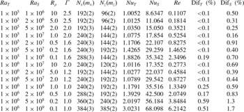
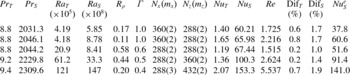
. The details of these simulations are summarised in table 1. Moreover, in order to make a direct comparison with the experiments, five cases from HT are numerically simulated with exactly the same parameters, which are summarised in table 2.
Summary of the simulations with
 $\mathit{Pr}_{T}=7$
and
 $\mathit{Pr}_{S}=700$
. The columns are, from left to right, the Rayleigh numbers of temperature and salinity, the density ratio, the aspect ratio of the domain, the resolutions in the horizontal and vertical directions (with refinement coefficients for multiple resolutions), the Nusselt numbers of temperature and salinity, the Reynolds number based on the root mean square (r.m.s.) value of velocity and the maximal differences between the Nusselt numbers computed by four methods. The meshes in the
 $y$
direction are the same as in the
 $x$
direction.

Summary of simulations of five experimental cases. The first two columns are the Prandtl numbers and the last column is the experimental measurement of
 $\mathit{Nu}_{S}$
. The other columns are the same as in table 1. The complete experimental results for these cases can be found in HT.

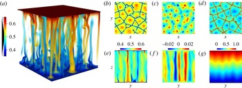
In all simulations thin salt fingers grow from the boundary layers adjacent to both plates and extend through the entire cell height. Slender convection cells develop along with the salt fingers. In figure 1(a) we show a three-dimensional visualisation of the salt fingers with
 $\mathit{Ra}_{T}=10^{6}$
and
 $\mathit{Ra}_{S}=2\times 10^{8}$
. The salty and fresh fingers are located alternately in space and correspond to individual convection cells. Near the top and bottom plates some sheet-like structures connect the roots of the fingers and form the boundaries of adjacent convection cells.
Instantaneous flow visualisation for the case with
 $\mathit{Ra}_{T}=1\times 10^{6}$
and
 $\mathit{Ra}_{S}=2\times 10^{8}$
. (a) Three-dimensional visualisation of salt fingers. Both the colour and the opacity are set by the salinity field. The red salty fingers grow from the top plate and extend to the bottom one, while the blue fresh fingers extend from the bottom plate to the upper one. (b–d) The contours of
 $s$
on the horizontal planes with
 $z=0.05L$
,
 $0.5L$
and
 $0.95L$
respectively. (e–g) The contours on a vertical section plane of salinity, vertical velocity and temperature respectively. Panels (b–d) have the same colourmap as (e).

To illustrate this more clearly, in figure 1(b–d) we show salinity contours on three cross sections:
 $z=0.05$
near the bottom plate,
 $z=0.5$
in the middle plane and
 $z=0.95$
near the top plate. Near both plates, the sheet-like structures are very distinct. The patterns are quite similar to those found in the sugar–salt experiments by Shirtcliffe & Turner (Reference Shirtcliffe and Turner1970). In the middle plane, the fingers take a nearly circular shape, although some weak links can be observed between fingers. This may explain why a ‘sheet-finger’ assumption generates a better representation of the experimental data than the ‘circular-finger’ assumption in HT. These flow visualisations also suggest that the periodic condition in the horizontal directions is appropriate, provided that there are enough salt fingers and convection cells in the computational domain. For the case
 $(\mathit{Ra}_{T},\mathit{Ra}_{S})=(10^{5},~5\times 10^{6})$
in table 1 we run a simulation with the same mesh size and half the domain size. The difference in the Nusselt numbers for the two domain sizes is smaller than 1 %. For all simulations
 ${\it\Gamma}$
is chosen so that the flow domain contains a similar number of convection cells.
Figure 1(e–g) depicts the different patterns of the salinity, velocity and temperature fields in a vertical plane. The salinity field has the smallest scale in the horizontal directions. Naturally, each salt finger is associated with a plume of high vertical velocity, which has a larger width than the salt finger. Due to its large diffusivity, the temperature field only exhibits wavy structures, and no thermal plumes can be found. The very different horizontal scales among various quantities verify the suitability and advantage of the double resolution method we used in our simulation.
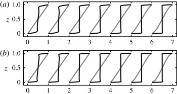
In figure 2 we plot the mean profiles
 $\overline{s}(z)$
and
 $\overline{{\it\theta}}(z)$
for the cases listed in table 1. The overline stands for an average over the time and
 $(x,y)$
planes. Clearly, the salinity field has two distinct boundary layers adjacent to both plates, and in between there is a bulk region with
 $\overline{s}$
of approximately 0.5. As
 $\mathit{Ra}_{S}$
increases, the thickness of the boundary layers decreases and the bulk region becomes more homogeneous. In contrast, there is no distinct division of the boundary layers and the bulk region in the temperature field. For given
 $\mathit{Ra}_{T}$
, when
 $\mathit{Ra}_{S}$
is small the mean temperature profile stays linear. Small deviations from the linear profile are only visible for large
 $\mathit{Ra}_{S}$
(equivalently small
 $R_{{\it\rho}}$
). This is reasonable since the fast diffusion of temperature (as compared with salinity) prevents the development of the small-scale structures.
Mean profiles of
 $s$
(black) and
 ${\it\theta}$
(grey) for cases in table 1: (a)
 $\mathit{Ra}_{T}=10^{5}$
and from left to right
 $\mathit{Ra}_{S}$
increases from
 $10^{6}$
to
 $10^{8}$
; (b)
 $\mathit{Ra}_{T}=10^{6}$
and from left to right
 $\mathit{Ra}_{S}$
increases from
 $10^{7}$
to
 $10^{9}$
. For clarity, each curve is shifted rightward by 1 from the previous one.

4. System response in the explored parameter space
The parameter space we have explored is shown in the
 $(\mathit{Ra}_{S},\mathit{Ra}_{T})$
plane in figure 3(a). The experimental cases of HT are also included in this figure. The cases listed in table 2, which serve for the direct comparison between the numerical and experimental results, are marked by grey (red online) crosses in the two parameter spaces. Together, our simulations and the HT experiments cover a
 $\mathit{Ra}_{S}$
range of over six decades and a
 $\mathit{Ra}_{T}$
range of over four decades.
Parameter space in the
 $\mathit{Ra}_{S}{-}\mathit{Ra}_{T}$
(a) and
 $\mathit{Ra}_{S}{-}R_{{\it\rho}}$
(b) planes. Circles, cases in table 1 with
 $\mathit{Ra}_{T}=10^{5}$
; squares, cases in table 1 with
 $\mathit{Ra}_{T}=10^{6}$
; black pluses, experiments from HT; grey (red online) crosses, cases listed in table 2. The same symbols will be used in all similar figures hereafter.

In figure 3(b) we plot the same parameter space in the
 $(\mathit{Ra}_{S},R_{{\it\rho}})$
plane. Here,
 $R_{{\it\rho}}$
measures the ratio of the stabilising force of the temperature field to the destabilising force of the salinity field. When
 $R_{{\it\rho}}\geqslant 1$
, the flow is in the traditional finger regime which has been studied extensively. When
 $R_{{\it\rho}}<1$
, the destabilising force of the salinity field is stronger than the stabilising force of the temperature field, thus the flow is more similar to RB flow. Most of the HT experiments are in the latter regime, and interestingly these authors found that fingers develop even with a very weak temperature difference. Schmitt (Reference Schmitt2011) extended the theory for the traditional finger regime to that with
 $R_{{\it\rho}}<1$
and revealed that a narrow finger solution may still exist. Here, in our simulation we systematically vary
 $R_{{\it\rho}}$
from 0.1 to 10, which covers both regimes.
As discussed in § 2, the Nusselt numbers for temperature and salinity are measured by four different methods. The final Nusselt numbers are the averages of these four values, which are given in tables 1 and 2. In these tables the maximal differences among the four values are also given. The maximal differences of
 $\mathit{Nu}_{T}$
and
 $\mathit{Nu}_{S}$
are less than 1 % for all the cases with
 $\mathit{Ra}_{S}<5\times 10^{8}$
. When
 $\mathit{Ra}_{S}\geqslant 5\times 10^{8}$
the differences increase but they are still below 2 %. This confirms the convergence of our simulations. For the Reynolds number we choose the characteristic velocity
 $U_{c}$
as the r.m.s. value of velocity computed with all three components.
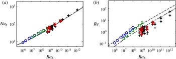
In figure 4(a,b) we plot the dependences of
 $\mathit{Nu}_{S}$
and
 $\mathit{Re}$
on
 $\mathit{Ra}_{S}$
respectively. It is clear that
 $\mathit{Nu}_{S}$
shows the same dependence on
 $\mathit{Ra}_{S}$
in the whole range considered here, despite the different Prandtl numbers in simulations and experiments. In our simulations we have four pairs of cases at
 $\mathit{Ra}_{S}=1\times 10^{7}$
,
 $2\times 10^{7}$
,
 $5\times 10^{7}$
and
 $1\times 10^{8}$
. Within each pair
 $\mathit{Ra}_{T}\in \{10^{5},10^{6}\}$
and we can see that
 $\mathit{Nu}_{S}$
is very similar, i.e. it has only a weak dependence on
 $\mathit{Ra}_{T}$
. Indeed, the symbols with same
 $\mathit{Ra}_{S}$
and different
 $\mathit{Ra}_{T}$
are very close to each other. Experimental results also show the same trend, especially in the higher
 $\mathit{Ra}_{S}$
region. For instance, in figure 4(a) at
 $\mathit{Ra}_{S}\approx 10^{11}$
there are actually four data points with
 $\mathit{Ra}_{T}$
ranging from
 $2.42\times 10^{7}$
to
 $9.7\times 10^{7}$
. This implies that
 $\mathit{Nu}_{S}$
depends mainly on
 $\mathit{Ra}_{S}$
and is only slightly affected by the change of
 $\mathit{Ra}_{T}$
.
Plots of
 $\mathit{Nu}_{S}$
(a) and
 $\mathit{Re}$
(b) versus
 $\mathit{Ra}_{S}$
for simulations and experiments. For the cases listed in table 2, the grey (red online) pluses represent the experimental results and the grey (red online) crosses represent the simulation results. The predictions of the GL model are given by the dashed line for
 $\mathit{Pr}_{S}=700$
and the dash dotted line for
 $\mathit{Pr}_{S}=2100$
. For
 $\mathit{Nu}_{S}$
these two lines almost collapse with each other (see (a)).

Changing
 $\mathit{Ra}_{T}$
while keeping
 $\mathit{Ra}_{S}$
fixed does have a notable influence on
 $\mathit{Re}$
, as shown in figure 4(b). For the same
 $\mathit{Ra}_{S}$
, larger
 $\mathit{Ra}_{T}$
generates smaller
 $\mathit{Re}$
. It should be recalled that
 $\mathit{Ra}_{S}$
measures the unstable driving force and
 $\mathit{Ra}_{T}$
represents the stabilising force of the temperature field. Then, fixing
 $\mathit{Ra}_{S}$
and increasing
 $\mathit{Ra}_{T}$
means that the stabilising force becomes relatively stronger, therefore a smaller
 $\mathit{Re}$
. The same phenomenon is also found in the HT experiments.
The cases in table 2 are marked by the grey (red online) crosses and plus symbols in figure 4. The grey (red online) crosses are numerical results and the grey (red online) pluses are experimental results from HT. As compared with the experiments, the numerical simulations generate larger
 $\mathit{Nu}_{S}$
. It seems that the discrepancy becomes smaller as the experimental Nusselt number
 $\mathit{Nu}_{S}^{e}$
increases. For the three cases with higher
 $\mathit{Nu}_{S}^{e}$
the discrepancy is below 10 %, which is within the uncertainty of experimental measurement. The discrepancy of
 $\mathit{Re}$
between experiments and simulations is larger than that of
 $\mathit{Nu}_{S}$
. This may be attributed to the way in which the r.m.s. velocity is computed. In HT the r.m.s. value was computed by using the velocity components within a vertical plane where the flow field was measured. Here, we compute the r.m.s. value by all three components and averaging over the entire domain. Since the salt fingers keep their position for a very long time, the r.m.s. value measured in the HT experiments depends on the location of the measured plane. Nonetheless, numerical results show a dependence of
 $\mathit{Re}$
on
 $\mathit{Ra}_{S}$
similar to experiments.
5. Effects of the temperature field
The density flux ratio, i.e. the ratio of the density anomaly flux due to temperature and that due to salinity, is defined as
 $$\begin{eqnarray}R_{f}=\frac{{\it\beta}_{T}\langle u_{3}{\it\theta}\rangle _{V}}{{\it\beta}_{S}\langle u_{3}s\rangle _{V}}=\mathit{Le}\,R_{{\it\rho}}\frac{\mathit{Nu}_{T}-1}{\mathit{Nu}_{S}-1}.\end{eqnarray}$$
Then, from (2.9c ) one can easily obtain
 $$\begin{eqnarray}{\it\epsilon}_{u}={\it\nu}^{3}L^{-4}\mathit{Ra}_{S}\,\mathit{Pr}_{S}^{-2}(\mathit{Nu}_{S}-1)(1-R_{f}).\end{eqnarray}$$
Thus, the temperature field affects the global balance between the momentum dissipation and the convection through the factor
 $1-R_{f}$
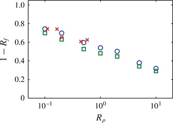
. In figure 5 we plot the variation of
 $1-R_{f}$
with
 $R_{{\it\rho}}$
. Since the HT experiments did not measure the heat flux, in the figure we only show the numerical results. This dependence is similar for all analysed
 $\mathit{Ra}_{T}$
(corresponding to different symbols in the figure). Namely, it decreases as
 $R_{{\it\rho}}$
increases. As
 $R_{{\it\rho}}\rightarrow 0$
, the influence of the temperature field becomes weaker and
 $R_{{\it\rho}}=0$
recovers the RB flow purely driven by the salinity difference. When
 $R_{{\it\rho}}\rightarrow \infty$
, the stabilising force of the temperature field becomes stronger and eventually there is no motion. For
 $R_{{\it\rho}}=10$
,
 $1-R_{f}$
is approximately 0.3. Therefore, the temperature field has quite a strong effect on momentum convection even when
 $\mathit{Nu}_{T}$
is much smaller than
 $\mathit{Nu}_{S}$
. This is again due to the huge difference between
 ${\it\lambda}_{T}$
and
 ${\it\lambda}_{S}$
, which is reflected by a large
 $\mathit{Le}$
in (5.1).


It should be pointed out that in our simulations
 $R_{f}$
increases as
 $R_{{\it\rho}}$
becomes larger, while it was reported in the literature that
 $R_{f}$
is inversely proportional to
 $R_{{\it\rho}}$
for
 $R_{{\it\rho}}>1$
and
 $R_{f}\rightarrow 1$
as
 $R_{{\it\rho}}\rightarrow 1$
, e.g. see the review of Kunze (Reference Kunze2003) and the references therein. The reason for this difference may be the different flow configurations. For most of the experiments and simulations examined by Kunze (Reference Kunze2003) the fingers start from an interface between two homogeneous layers and grow freely during time. However, for our configuration the maximal vertical length of the fingers is limited to the height between the two plates, and indeed for all the parameters we simulated the fingers extend from one boundary layer to the opposite one and they have almost the same height.
To further reveal the effects of the temperature field, we simulated another two cases for
 $\mathit{Ra}_{S}=10^{7}$
. The first one has
 $\mathit{Ra}_{T}=10^{3}$
and the other has no temperature field, namely pure RB flow. We obtain
 $\mathit{Nu}_{S}=17.431$
and 17.249 respectively. These values are very close to the two cases with the same
 $\mathit{Ra}_{S}$
in table 1, i.e.
 $\mathit{Nu}_{S}=17.854$
with
 $\mathit{Ra}_{T}=10^{5}$
and
 $\mathit{Nu}_{S}=17.352$
with
 $\mathit{Ra}_{T}=10^{6}$
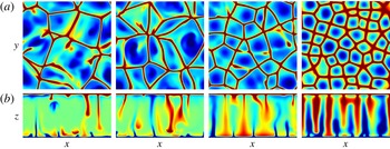
. Figure 6 compares the salinity fields for these four cases with different
 $\mathit{Ra}_{T}$
. It can be seen that as
 $\mathit{Ra}_{T}$
increases, the horizontal size of the convection cells shrinks. In the RB flow shown in the left column, the salt plumes from one plate become very weak before they reach the opposite plate. For larger
 $\mathit{Ra}_{T}$
the plumes are stronger and grow more vertically. Finally, almost all plumes reach the opposite plate and form salt fingers. Therefore, with the stabilising effect of the temperature field, the large-scale flows in the pure RB case are prevented and the salt fingers tend to move vertically.
Comparison of salinity fields for fixed
 $\mathit{Ra}_{S}=10^{7}$
and different values of
 $\mathit{Ra}_{T}$
. From left to right: RB flow,
 $\mathit{Ra}_{T}=10^{3}$
,
 $\mathit{Ra}_{T}=10^{5}$
and
 $\mathit{Ra}_{T}=10^{6}$
. (a) Horizontal sections at
 $z=0.95$
near the top plate; (b) vertical sections. For all plots the colourmap is the same as in figure 1(e).

The above observations imply that the temperature field does change the morphology of the salinity field, such as the horizontal size of the salt fingers and convection cells. It should be recalled that
 $\mathit{Re}$
has a notable dependence on
 $\mathit{Ra}_{T}$
, while the dependence of
 $\mathit{Nu}_{S}$
on
 $\mathit{Ra}_{T}$
is very weak. Thus, it seems that the temperature field affects the size of the salt fingers and the speed of the flow motion in such a way that the salinity flux stays fixed for certain
 $\mathit{Ra}_{S}$
.
6. The GL theory applied to DDC
The GL theory developed by Grossmann & Lohse (Reference Grossmann and Lohse2000, Reference Grossmann and Lohse2001, Reference Grossmann and Lohse2002, Reference Grossmann and Lohse2004) successfully accounts for the
 $\mathit{Ra}$
and
 $\mathit{Pr}$
dependence of
 $\mathit{Nu}$
and
 $\mathit{Re}$
for RB flow. The starting point of the theory is two exact relations for the kinetic and thermal energy dissipation rates (the analogues of (2.9)). The volume averages of the dissipation rates are then divided into the contributions of the bulk region and of the boundary layers, which both can then be modelled individually, leading to
 $$\begin{eqnarray}\displaystyle (\mathit{Nu}-1)\mathit{Ra}\mathit{Pr}^{-2}=c_{1}\frac{\mathit{Re}^{2}}{g\left(\sqrt{\mathit{Re }_{c}/\mathit{Re}}\right)}+c_{2}\mathit{Re}^{3}, & & \displaystyle\end{eqnarray}$$
 $$\begin{eqnarray}\displaystyle \mathit{Nu}-1=c_{3}\mathit{Re}^{1/2}\,\mathit{Pr}^{1/2}\left\{f\left[\frac{2a\mathit{Nu}}{\sqrt{\mathit{Re }_{c}}}g\left(\sqrt{\frac{\mathit{Re }_{c}}{\mathit{Re}}}\right)\right]\right\}^{1/2}+\displaystyle c_{4}\mathit{Re}\,\mathit{Pr}f\left[\frac{2a\mathit{Nu}}{\sqrt{\mathit{Re }_{c}}}g\left(\sqrt{\frac{\mathit{Re }_{c}}{\mathit{Re}}}\right)\right], & & \displaystyle \nonumber\\ \displaystyle & & \displaystyle\end{eqnarray}$$
 $\mathit{Re}_{c}=4a^{2}$
as the critical Reynolds number, describing the transition to the large-
 $Pr$
regime (Grossmann & Lohse Reference Grossmann and Lohse2002). The model has five coefficients, i.e.
 $a$
and
 $c_{i}$
with
 $i=1,2,3,4$
. Their values are
 $c_{1}=8.05$
,
 $c_{2}=1.38$
,
 $c_{3}=0.487$
,
 $c_{4}=0.0252$
and
 $a=0.922$
, with which
 $Nu(Ra,Pr)$
and
 $Re(Ra,Pr)$
can very well be described (Stevens et al.
Reference Stevens, van der Poel, Grossmann and Lohse2013).
In generalisation of this concept, now all three dissipation rates (2.9) are split into bulk and BL contributions as
 $$\begin{eqnarray}\displaystyle & {\it\epsilon}_{u}={\it\epsilon}_{u,BL}+{\it\epsilon}_{u,bulk}, & \displaystyle\end{eqnarray}$$
 $$\begin{eqnarray}\displaystyle & {\it\epsilon}_{{\it\theta}}={\it\epsilon}_{{\it\theta},BL}+{\it\epsilon}_{{\it\theta},bulk}, & \displaystyle\end{eqnarray}$$
 $$\begin{eqnarray}\displaystyle & {\it\epsilon}_{s}={\it\epsilon}_{s,BL}+{\it\epsilon}_{s,bulk}. & \displaystyle\end{eqnarray}$$
 $$\begin{eqnarray}\displaystyle (\mathit{Nu}_{S}-1)\mathit{Ra}_{S}\mathit{Pr}_{S}^{-2}+(\mathit{Nu}_{T}-1)\mathit{Ra}_{T}\mathit{Pr}_{T}^{-2}=c_{1}\frac{\mathit{Re}^{2}}{g\left(\sqrt{\mathit{Re }_{c}/\mathit{Re}}\right)}+c_{2}\mathit{Re}^{3}, & & \displaystyle\end{eqnarray}$$
 $$\begin{eqnarray}\displaystyle \mathit{Nu}_{T}-1 & = & \displaystyle c_{3,{\it\theta}}\mathit{Re}^{1/2}\,\mathit{Pr}_{T}^{1/2}\left\{f\left[\frac{2a\mathit{Nu}_{T}}{\sqrt{\mathit{Re }_{c}}}g\left(\sqrt{\frac{\mathit{Re }_{c}}{\mathit{Re}}}\right)\right]\right\}^{1/2}\nonumber\\ \displaystyle & & \displaystyle +\,\displaystyle c_{4,{\it\theta}}\mathit{Re}\,\mathit{Pr}_{T}f\left[\frac{2a\mathit{Nu}_{T}}{\sqrt{\mathit{Re }_{c}}}g\left(\sqrt{\frac{\mathit{Re }_{c}}{\mathit{Re}}}\right)\right],\end{eqnarray}$$
 $$\begin{eqnarray}\displaystyle \mathit{Nu}_{S}-1 & = & \displaystyle c_{3,s}\mathit{Re}^{1/2}\,\mathit{Pr}_{S}^{1/2}\left\{f\left[\frac{2a\mathit{Nu}_{S}}{\sqrt{\mathit{Re }_{c}}}g\left(\sqrt{\frac{\mathit{Re }_{c}}{\mathit{Re}}}\right)\right]\right\}^{1/2}\nonumber\\ \displaystyle & & \displaystyle +\,\displaystyle c_{4,s}\mathit{Re}\,\mathit{Pr}_{S}f\left[\frac{2a\mathit{Nu}_{S}}{\sqrt{\mathit{Re }_{c}}}g\left(\sqrt{\frac{\mathit{Re }_{c}}{\mathit{Re}}}\right)\right].\end{eqnarray}$$
 $c_{1}$
,
 $c_{2}$
,
 $c_{3,{\it\theta}}$
,
 $c_{4,{\it\theta}}$
,
 $c_{3,s}$
,
 $c_{4,s}$
and
 $a$
would have to be obtained from a fit to experimental or numerical data. However, it is much easier in this case: they can be deduced from the limiting cases for which of course the same constants hold as in the general case. Imagine
 $Ra_{S}=0$
, i.e. only thermal driving. Then (6.3) reduces to (6.1) with
 $c_{3,{\it\theta}}=c_{3}$
and
 $c_{4,{\it\theta}}=c_{4}$
, i.e. the known values. Next, imagine
 $Ra_{T}=0$
, i.e. only salinity driving. Then the salinity field takes the role of the thermal field in the standard RB case and thus (6.3) again reduces to (6.1), with
 $c_{3,s}=c_{3}$
and
 $c_{4,s}=c_{4}$
, i.e. again the known values! Moreover, as by construction of the model the prefactors do not depend on the control parameters
 $\mathit{Ra}_{T}$
,
 $\mathit{Ra}_{S}$
,
 $\mathit{Pr}_{T}$
,
 $\mathit{Pr}_{S}$
, these equalities not only hold in the limiting cases but throughout and we have in general
 $$\begin{eqnarray}c_{3,{\it\theta}}=c_{3,s}=c_{3}\quad \text{and}\quad c_{4,{\it\theta}}=c_{4,s}=c_{4}\end{eqnarray}$$
with the known values for
 $c_{3}$
and
 $c_{4}$
and also for
 $c_{1}$
,
 $c_{2}$
and
 $a$
(Stevens et al.
Reference Stevens, van der Poel, Grossmann and Lohse2013).
If the flow is driven by one component and stabilised by the other one, which is the case in the present study, the driving component can still be modelled in the same fashion as in (6.3), but the other component must be modelled differently. However, as we discussed in the previous section,
 $\mathit{Ra}_{T}$
only has a minor effect on the salinity transfer
 $\mathit{Nu}_{S}$
in our problem. Moreover, the temperature field shows no clear distinction between the boundary layer region and the bulk region, as indicated by the temperature field in figure 1(g) and the mean profiles in figure 2. Thus, one can neglect the thermal terms in model (6.3) and still obtain accurate predictions of the salinity transfer.
With the original values of the coefficients,
 $\mathit{Nu}_{S}(\mathit{Ra}_{S})$
has been computed for
 $\mathit{Pr}_{S}=700$
and 2100, which are shown by lines in figure 4(a). Indeed, the GL predictions agree excellently with both numerical and experimental results in the whole range of
 $10^{6}<\mathit{Ra}_{S}<10^{12}$
. The two lines with different values of
 $\mathit{Pr}_{S}$
have only a slight difference. This is similar to the RB flow where the Nusselt number saturates when the Prandtl number is large enough. We want to emphasise that no new parameters are introduced and the model developed for RB flow also works remarkably well for the present DDC flow.
What about the dependence of the Reynolds numbers on the control parameters? As pointed out by Grossmann & Lohse (Reference Grossmann and Lohse2002), the distribution
 $\mathit{Nu}_{S}(\mathit{Ra}_{S},\mathit{Pr}_{S})$
is invariant under the transformation
 $$\begin{eqnarray}a\rightarrow {\it\alpha}^{1/2}a,\quad c_{1}\rightarrow c_{1}/{\it\alpha}^{2},\quad c_{2}\rightarrow c_{2}/{\it\alpha}^{3},\quad c_{3}\rightarrow c_{3}/{\it\alpha}^{1/2},\quad c_{4}\rightarrow c_{4}/{\it\alpha}.\end{eqnarray}$$
Following the procedure of Stevens et al. (Reference Stevens, van der Poel, Grossmann and Lohse2013), we use one case to fix the transformation coefficient
 ${\it\alpha}$
and thus rescale the Reynolds number
 $\mathit{Re}(\mathit{Ra}_{S},\mathit{Pr}_{S})$
to the present flow. By using the Reynolds number of the case with
 $(\mathit{Ra}_{T},\mathit{Ra}_{S})=(10^{5},10^{7})$
,
 ${\it\alpha}$
is determined as 0.126. The GL prediction of
 $\mathit{Re}(\mathit{Ra}_{S})$
is then computed with the transformed coefficients for
 $\mathit{Pr}_{S}=700$
and 2100, which is shown in figure 4(b). The theoretical lines show reasonable agreement with simulations and experiments. Since the effect of the temperature field is not included in the present model, thus the dependence of
 $\mathit{Re}$
on
 $\mathit{Ra}_{T}$
is absent in the theoretical prediction.
Figure 4 demonstrates the success of our approach. As theoretically argued, it is indeed possible to apply the GL model with the known parameters for RB flow to DDC flow. The model not only captures the variation trends of
 $\mathit{Nu}_{S}$
and
 $\mathit{Re}$
, but also shows quantitive agreement with numerical and experimental data on the log–log plot.
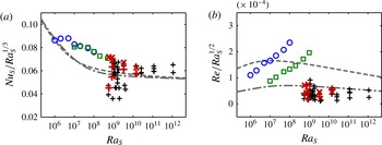
Compensated plots of
 $\mathit{Nu}_{S}$
and
 $\mathit{Re}$
versus
 $\mathit{Ra}_{S}$
. The lines and symbols are the same as in figure 4.

In order to compare the model and the data more precisely, we plot the data and model predictions in a compensated way. Namely,
 $\mathit{Nu}_{S}$
and
 $\mathit{Re}$
are respectively compensated by
 $\mathit{Ra}_{S}^{-1/3}$
and by
 $\mathit{Ra}_{S}^{-1/2}$
. The results are shown in figure 7. Here, we see that our approach also inherits some weaknesses of the original GL model: looking in this detail it becomes clear that
 $\mathit{Nu}_{S}$
follows a trend different from the model, especially when
 $\mathit{Ra}_{S}<10^{9}$
. A similar discrepancy between the original GL model and experimental data was also observed for RB flow at very large Prandtl number, e.g. see figure 7 of Stevens et al. (Reference Stevens, van der Poel, Grossmann and Lohse2013). The difference between the GL model and the data is even larger for the Reynolds numbers of the cases in table 1, as shown by the circles and dashed line in figure 7(b). Surprisingly, the model prediction of
 $\mathit{Re}$
shows a reasonable agreement with the HT experiments even in the compensated plot.
In closing this section, we would like to point out that the scaling laws given by Hage & Tilgner (Reference Hage and Tilgner2010), which also capture the behaviour of the present numerical and experimental data, exhibit a similar transition around
 $\mathit{Ra}_{S}\approx 10^{9}$
when plotted in the compensated way as in figure 7 (not shown here). Therefore, the discrepancy at
 $\mathit{Ra}_{S}<10^{9}$
requires further investigation in future work.
7. Conclusions
In conclusion, DDC flow was studied numerically for a series of flow parameters, using a flow configuration similar to that of the experiments by HT, in which the convection was driven by a salinity difference between two plates and stabilised by a temperature difference. Direct comparison was made between experiments and numerical simulations for several sets of parameters, and reasonable agreement was achieved for the salinity flux. Salt fingers exist in all the simulations. Flow visualisations show that the saltier and fresher fingers grow from the top and bottom plates respectively, and extend to the opposite boundary layer. They are associated with slender convection cells. Near the plate where the saltier or fresher fingers grow, they usually originate from sheet-like structures. When the fingers reach the opposite plate, they are bounded by the sheet-like structures near that plate. These sheet-like structures are quite weak in the bulk region. This justifies the ‘sheet-finger’ assumption of HT.
Both our numerical results and the experimental results of HT exhibit the same dependence of
 $\mathit{Nu}_{S}$
on
 $\mathit{Ra}_{S}$
. For the present configuration, the change of
 $\mathit{Ra}_{T}$
has a minor influence on
 $\mathit{Nu}_{S}$
but affects
 $\mathit{Re}$
. To provide a new interpretation of the dependences of
 $\mathit{Nu}_{S}$
and
 $\mathit{Re}$
on
 $\mathit{Pr}_{S}$
and
 $\mathit{Ra}_{S}$
, we directly apply the GL theory for RB flow to the present problem. Without any modification of the coefficients, the theory successfully predicts
 $\mathit{Nu}_{S}(\mathit{Pr}_{S},\mathit{Ra}_{S})$
with quite good accuracy for both numerical and experimental results in the
 $\mathit{Ra}_{S}$
range of
 $(10^{6},10^{12})$
. The
 $\mathit{Re}(\mathit{Pr}_{S},\mathit{Ra}_{S})$
predictions of the theory and the data also show reasonable agreement, especially for the experimental results.
The effects of the temperature field are also discussed for the present flow configuration. The temperature field changes the morphology of the salt fingers but has a minor influence on the salinity flux. It is remarkable that the Nusselt number of pure RB flow is very close to that of double diffusive flow when the unstable component field has the same Prandtl and Rayleigh numbers.
Finally, it should be pointed out that the present model does not include the influence of
 $\mathit{Ra}_{T}$
and
 $\mathit{Pr}_{T}$
. Thus, it cannot predict the behaviour of
 $\mathit{Nu}_{T}$
, neither can it describe the dependence of
 $\mathit{Re}$
on
 $\mathit{Ra}_{T}$
. Thus, an extension of the GL model would be needed in future work to fully cooperate with the DDC problem.
Acknowledgements
This study is supported by FOM and the National Computing Facilities (NCF), both sponsored by NWO, and ERC.