1 Introduction
Axisymmetric jets have been the subject of numerous studies in the past due to their common use as mixing and thrust producing devices (Ho & Gutmark Reference Ho and Gutmark1987). An axisymmetric round jet issuing directly from a contraction produces a flat-topped (‘top-hat’) velocity profile in the near field and develops towards a turbulent state in the far field by entraining and mixing background (quiescent) fluid into the turbulent stream. Entrainment describes a process through which there is an exchange of momentum, energy, vorticity, mass and other properties between the surrounding fluid and the turbulent stream across the sharp turbulent/non-turbulent interface (TNTI). This process can take place in two ways, through engulfment (ingestion of irrotational fluid into the turbulent stream) and nibbling (small-scale diffusion across the interface). These two processes do not exclude each other and based on the state of any coherent structures embedded within the flow one may be more important than the other. Establishing which process is dominant across the evolution of the jet is somewhat open to debate (da Silva et al. Reference da Silva, Hunt, Eames and Westerweel2014), since some authors have suggested that in turbulent jets engulfment is dominant, whilst others have pointed to nibbling. Dahm & Dimotakis (Reference Dahm and Dimotakis1987) and Dimotakis (Reference Dimotakis2000) suggested that engulfment would be the dominant process in the far field of axisymmetric jets and a similar conclusion was reached by Mungal, Karasso & Lonzano (Reference Mungal, Karasso and Lonzano1991) for diffusion flames. Contrastingly, Westerweel et al. (Reference Westerweel, Fukushima, Pedersen and Hunt2005) pointed to nibbling as the dominant entrainment process in the far field of a jet between 60 and 100 jet diameters downstream of the exit.
Examining the state of the TNTI has posed significant challenges in the past due to its very small thickness. The first significant work on this topic (Corrsin & Kistler Reference Corrsin and Kistler1954) suggested the existence of a viscous laminar superlayer (VSL) which matched the irrotational background to the turbulent, vortical flow. Corrsin & Kistler (Reference Corrsin and Kistler1954) suggested that the thickness of this layer would scale with a viscous length scale, usually assumed to be the Kolmogorov length scale
 $\unicode[STIX]{x1D702}$
. Note that the outer-most extremity of the TNTI/viscous superlayer is usually referred to as the irrotational boundary. Decades later, works have suggested that the TNTI is not only composed of the VSL, but also of a turbulent sublayer (TSL) where the vorticity reaches a local maximum and which has a thickness that scales with the Taylor length scale
 $\unicode[STIX]{x1D706}_{f}$
(Bisset, Hunt & Rogers Reference Bisset, Hunt and Rogers2002; van Reeuwijk & Holzner Reference van Reeuwijk and Holzner2014) or simply to the radius of the large-scale vortical structures (LVS) near the interface (da Silva & Taveira Reference da Silva and Taveira2010).
Traditionally, the smallest scales present in a turbulent flow have been thought to be independent of the large scales, however recent work, particularly at modest Reynolds number, has started to cast doubt on this (Buxton Reference Buxton2015; Fiscaletti et al. Reference Fiscaletti, Attili, Bisetti and Elsinga2016a ,Reference Fiscaletti, Elsinga, Attili, Bisetti and Buxton b ). This gives rise to the possibility that as well as directly influencing the engulfment into a turbulent jet the large-scale coherent structures may also indirectly influence entrainment through small-scale nibbling processes, for example if the small scales are ‘slaved’ to the large scales. In this manuscript we examine this by comparing a ‘classic’ round jet with a particular non-circular exit geometry – a repeating fractal pattern. Breda & Buxton (Reference Breda and Buxton2018a ,Reference Breda and Buxton b ) recently compared axisymmetric jets fitted with a circular and fractal-shaped orifice with identical open area and at identical Reynolds numbers and showed that the fractal jet substantially suppressed the coherent structures in the near field of the jet in relation to the round jet. In particular, they showed that this modified the entrainment rate into the jet’s near field before both jets evolved into an axisymmetric self-similar state further downstream. The objective of this manuscript is thus to try and link this modified entrainment rate to the behaviour of the TNTI and properties of the small-scale turbulence in the near-interface region of these two jets.
The behaviour of the small scales will be examined through the velocity-gradient tensor (VGT), which can be split into a symmetric and skew-symmetric part (or a strain-rate and rotation tensor),
 $$\begin{eqnarray}\displaystyle & \displaystyle \unicode[STIX]{x1D622}_{ij}=\frac{\unicode[STIX]{x2202}u_{i}}{\unicode[STIX]{x2202}x_{j}}=\unicode[STIX]{x1D634}_{ij}+\unicode[STIX]{x1D714}_{ij}=\frac{1}{2}\left(\frac{\unicode[STIX]{x2202}u_{i}}{\unicode[STIX]{x2202}x_{j}}+\frac{\unicode[STIX]{x2202}u_{j}}{\unicode[STIX]{x2202}x_{i}}\right)+\frac{1}{2}\left(\frac{\unicode[STIX]{x2202}u_{i}}{\unicode[STIX]{x2202}x_{j}}-\frac{\unicode[STIX]{x2202}u_{j}}{\unicode[STIX]{x2202}x_{i}}\right). & \displaystyle\end{eqnarray}$$
Here the flow velocity is split into its mean and fluctuating part following the Reynolds decomposition
 $U_{i}=\overline{U_{i}}+u_{i}$
. Chong, Perry & Cantwell (Reference Chong, Perry and Cantwell1990) and Chacin & Cantwell (Reference Chacin and Cantwell2000) defined the invariants of the VGT, so called because they remain constant regardless of which coordinate system is used, from the roots of the characteristic equation for
 $\unicode[STIX]{x1D622}_{ij}$
written as
 $$\begin{eqnarray}\displaystyle \unicode[STIX]{x1D709}^{3}+P\unicode[STIX]{x1D709}^{2}+Q\unicode[STIX]{x1D709}+R=0, & & \displaystyle\end{eqnarray}$$
where
 $P$
,
 $Q$
and
 $R$
are the invariants. The first invariant
 $P$
describes the negative trace of the VGT (
 $P=-\unicode[STIX]{x1D622}_{ii}$
) and is therefore zero for an incompressible flow, hence leaving
 $Q$
and
 $R$
to describe the flow topology
 $$\begin{eqnarray}\displaystyle & \displaystyle Q={\textstyle \frac{1}{4}}(\unicode[STIX]{x1D714}_{i}\unicode[STIX]{x1D714}_{i}-2\unicode[STIX]{x1D634}_{ij}\unicode[STIX]{x1D634}_{ij})=Q_{\unicode[STIX]{x1D714}}+Q_{s}, & \displaystyle\end{eqnarray}$$
 $$\begin{eqnarray}\displaystyle & \displaystyle R=-{\textstyle \frac{1}{3}}\left(\unicode[STIX]{x1D634}_{ij}\unicode[STIX]{x1D634}_{jk}\unicode[STIX]{x1D634}_{ki}+{\textstyle \frac{3}{4}}\unicode[STIX]{x1D714}_{i}\unicode[STIX]{x1D634}_{ij}\unicode[STIX]{x1D714}_{j}\right)=R_{s}+R_{\unicode[STIX]{x1D714}}, & \displaystyle\end{eqnarray}$$
where
 $\unicode[STIX]{x1D714}_{i}$
is the
 $i$
th component of the vorticity vector. The invariant
 $Q$
can be considered as the local excess of swirling over strain rate, with its constituent parts
 $Q_{\unicode[STIX]{x1D714}}$
being half the magnitude of the enstrophy whilst
 $Q_{s}=-\unicode[STIX]{x1D700}/4\unicode[STIX]{x1D708}$
is proportional to the turbulent kinetic energy dissipation rate
 $\unicode[STIX]{x1D700}$
. Since
 $P=0$
,
 $Q$
and
 $R$
can be used to describe the state of an incompressible fluid element.
The joint probability density function (j.p.d.f.) of
 $Q$
and
 $R$
has been found to have a characteristic ‘tear-drop’ shape in a variety of ‘fully developed’ turbulent flows including homogeneous isotropic turbulence, mixing layers and wall-bounded flows (Soria et al.
Reference Soria, Sondergaard, Cantwell, Chong and Perry1994; Blackburn, Mansour & Cantwell Reference Blackburn, Mansour and Cantwell1996; Tsinober Reference Tsinober2009; Buxton & Ganapathisubramani Reference Buxton and Ganapathisubramani2010). This ‘ubiquity’ led to the belief that the tear-drop shaped j.p.d.f. is a universal signature of ‘fully developed’ fine-scale turbulent motions (Chacin & Cantwell Reference Chacin and Cantwell2000; Elsinga & Marusic Reference Elsinga and Marusic2010). Recently, however, Buxton, Breda & Chen (Reference Buxton, Breda and Chen2017) has observed this tear-drop shaped distribution of
 $Q$
and
 $R$
in the inhomogeneous, spatially developing near-wake region downstream of a square cylinder, suggesting that it may be more ubiquitous than previously thought. Contrastingly, Gomes-Fernandes, Ganapathisubramani & Vassilicos (Reference Gomes-Fernandes, Ganapathisubramani and Vassilicos2014) and Paul, Papadakis & Vassilicos (Reference Paul, Papadakis and Vassilicos2017) found that the tear-drop shape developed with distance downstream from a fractal-square grid and single-scale grid, respectively. In this manuscript we will also document the spatial development of the
 $Q$
–
 $R$
distribution, if it exists, in the round and fractal jets we examine, both in the streamwise direction and in the TNTI-normal direction, i.e. moving from the interface itself into the turbulent bulk. The objective will be to assess what, if any, effect the different state of the coherence in the near fields of the different jets has on the evolution of this
 $Q$
–
 $R$
distribution towards a ‘fully developed’ state.
2 Methodology
2.1 Jet structure
The flow was generated by an open jet facility at Imperial College London, previously described in Breda & Buxton (Reference Breda and Buxton2018a
,Reference Breda and Buxton
b
). In order to prevent biasing the particle images with unseeded, quiescent air becoming entrained into the jet a seeded, mild co-flow of air was used as described in Breda & Buxton (Reference Breda and Buxton2018a
,Reference Breda and Buxton
b
). The exit flow was found to have a sharp ‘top-hat’ mean velocity profile and turbulence intensity
 ${<}1\,\%$
. Two different orifices (round and fractal) of thickness 0.1 mm and of identical open area
 $D_{e}^{2}$
(
 $D_{e}=15.78~\text{mm}$
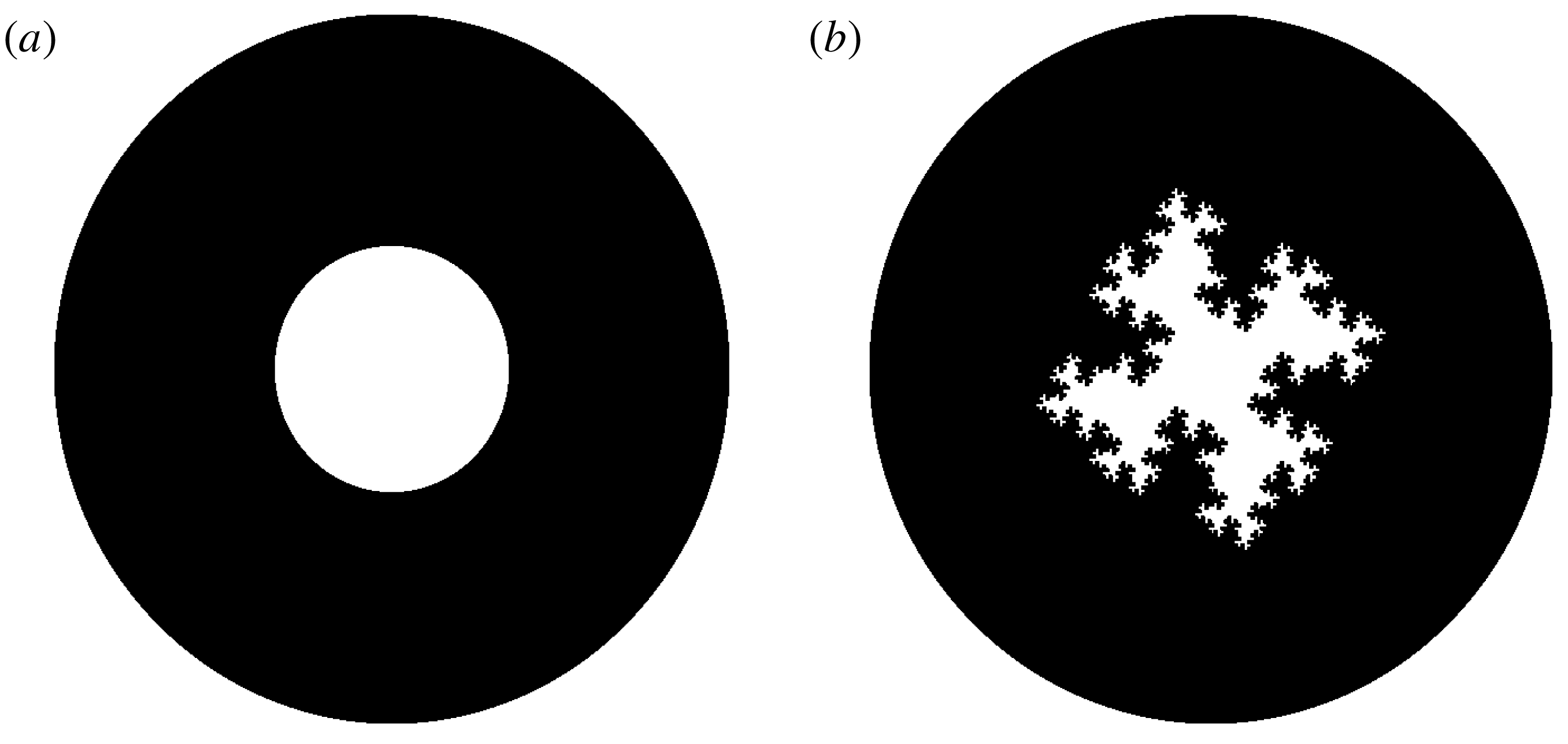
) were attached to the nozzle, as shown in figure 1. The repeating fractal pattern was formed of three iterations and has a fractal dimension of
 $D_{f}=1.5$
, first described in Nedić, Vassilicos & Ganapathisubramani (Reference Nedić, Vassilicos and Ganapathisubramani2013). Each jet thus has the same exit flow velocity
 $U_{e}=9.93~\text{m}~\text{s}^{-1}$
for a given volumetric flow rate,
 $$\begin{eqnarray}\displaystyle & \displaystyle D_{e}=\sqrt{\text{Exit area}},\quad U_{e}=\frac{\text{Volumetric flow rate}}{\text{Exit area}}, & \displaystyle\end{eqnarray}$$
meaning that the Reynolds number was kept the same for both jets, defined as
 $$\begin{eqnarray}\displaystyle & \displaystyle Re_{G}=\frac{U_{e}D_{e}}{\unicode[STIX]{x1D708}}=10^{4}. & \displaystyle\end{eqnarray}$$
The flow rates through the jet were carefully controlled using an Omega FMA-26 mass flow controller to ensure that these operating conditions were repeatable.
Exit geometries studied, (a) round and (b) fractal.

2.2 Nomenclature and coordinate system
The data from the tomographic particle image velocimetry (TPIV) experiments were acquired in a Cartesian coordinate system. This coordinate system is defined with
 $x$
as the streamwise component and
 $y$
and
 $z$
the orthogonal ones. The instantaneous velocities are
 $U$
,
 $V$
and
 $W$
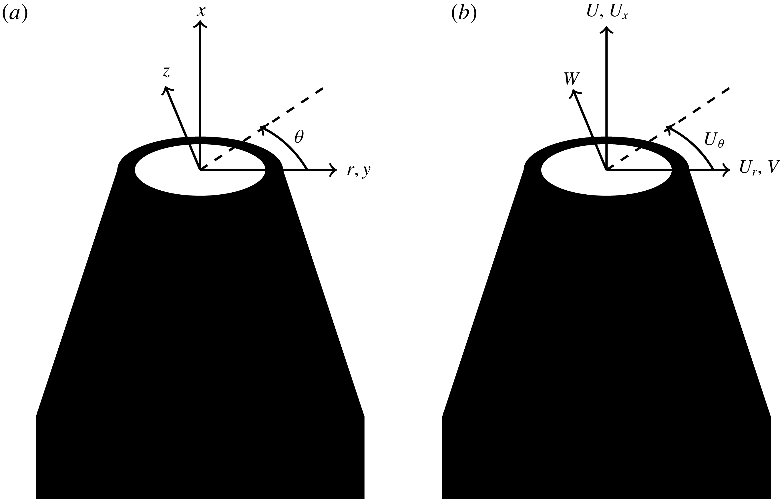
respectively. In some places the Cartesian coordinate system has been converted to a cylindrical one. In that case,
 $r$
is used to indicate the radial component, whilst
 $\unicode[STIX]{x1D703}$
indicates the azimuthal one. In the potential core, where the round jet has a ‘top-hat’ velocity profile, the location of the jet centre (
 $r=0$
) was determined as the minimum value of the root-mean-square of the streamwise velocity fluctuations. After the azimuthal shear layer coalesces, the location of the jet centre was determined by fitting a Gaussian curve to the streamwise mean velocity profile to find the maximum value. The instantaneous velocity components were then converted to
 $U_{x}$
,
 $U_{r}$
and
 $U_{\unicode[STIX]{x1D703}}$
, as shown in figure 2. The mean (time average) and fluctuating velocity are subsequently decomposed following the Reynolds decomposition.
(a) Jet’s coordinate system for the tomographic particle image velocimetry data and (b) velocity components.

2.3 Tomographic particle image velocimetry
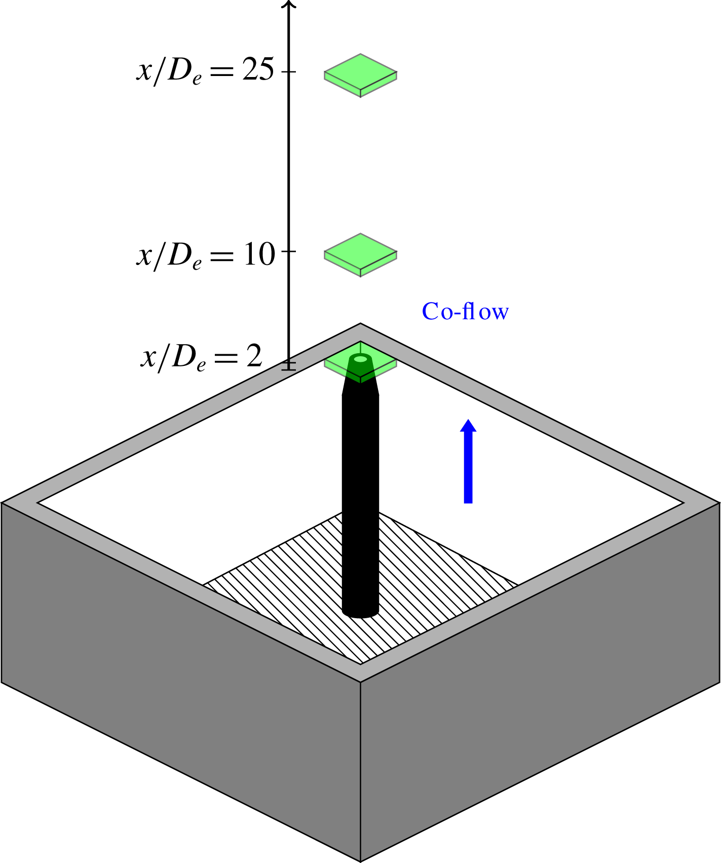
Schematics of volumes studied with TPIV.

The tomographic PIV (TPIV) interrogation volumes were centred on
 $x/D_{e}=2$
,
 $x/D_{e}=10$
and
 $x/D_{e}=25$
to study the spatial evolution of the velocity-gradient statistics of the jet, as shown in figure 3. The three regions were chosen to study the jet in three different phases (Breda & Buxton Reference Breda and Buxton2018b
):
(i)
 $x/D_{e}=2$
: here the jets are in a state of development. The first Kelvin–Helmholtz vortex rings have already developed and the turbulent kinetic energy is in a production phase, where the velocity fluctuations increase with streamwise distance
$x$
.
(ii)
$x/D_{e}=10$
: the azimuthal shear layer has coalesced and both round and fractal jet have passed the peak of turbulent kinetic energy (along the centreline).(iii)
$x/D_{e}=25$
: the mean velocity and Reynolds stresses are self-similar.


Keeping the illuminated volume’s thickness to a minimum allows an increased seeding density to be used and hence improves the spatial resolution, which is important to study the velocity gradients. The illuminated-volume thickness was set to be 5 mm (of which
 ${\approx}3~\text{mm}$
was retained after the PIV processing) with a variable aperture slit in order to compromise between a reasonable spatial resolution and thick enough volume depth whilst ensuring a sharp light intensity gradient at the edge of the volume.
This thickened light sheet was generated by a double cavity Nd:YAG low speed laser running at 15 Hz. The images were acquired with four cameras, 4 Megapixel Imager SX fitted with four lenses of type AF DC-Nikkor 105 mm f/2D (f-number f/16). An optical calibration was performed by traversing a dotted plate across the whole volume at the positions
 $\tilde{x}=0~\text{mm}$
, 2.5 mm and 5 mm and acquiring an image from the cameras in each step. (Here,
 $\tilde{x}=2.5~\text{mm}$
is the approximate centre of the laser volume at a given measurement station.) The commercial software DaVis was then used to generate the optical three-dimensional calibration knowing the distance between the three streamwise views. In order to improve the calibration quality, a volume self-calibration was completed as discussed by Wieneke (Reference Wieneke2008). In order to have a homogeneous disparity map, the images were recorded running the co-flow only. After these initial calibrations, images were acquired switching both the co-flow and jet on. The TPIV images were processed using the MART algorithm (6 iterations), a multiplicative algebraic reconstruction (Herman & Lent Reference Herman and Lent1976).
In order to improve the quality of the reconstruction of the images a dark background, previously acquired, was subtracted. Sliding minimum subtraction, Gaussian smoothing using a
 $3\times 3$
pixels kernel to reduce the background noise and sharpening to reduce the number of ‘ghost particles’ were also performed on the raw images, allowing the particle diameter to be of the order of 2 pixels and the ppp (particles per pixel) to be within 0.04–0.05. In order to reduce the processing time sparse cross-correlation (Discetti & Astarita Reference Discetti and Astarita2012) was implemented.
The vectors were reconstructed in three steps: an initial recursive direct correlation, followed by two iterations of motion tracking enhancement (MTE) (Novara, Batenburg & Scarano Reference Novara, Batenburg and Scarano2010) to reduce the number of ‘ghost particles’ and a final recursive direct correlation. (The first recursive direct correlation was done in steps of specific correlation volume voxel size (passes):
 $160\times 160\times 160(10)\rightarrow 96\times 96\times 96(2)\rightarrow 64\times 64\times 64(2)$
. The volume overlap was 75 %.) (The second recursive direct correlation was:
 $160\times 160\times 160(10)\rightarrow 96\times 96\times 96(2)\rightarrow 64\times 64\times 64(2)\rightarrow 48\times 48\times 48(2)$
. The volume overlap was 75 %.)
Finally, in order to correct the non-zero divergence of the resultant velocity fields, the data were corrected using the divergence correction scheme (DCS) of De Silva, Philip & Marusic (Reference De Silva, Philip and Marusic2013). This non-zero divergence is due to experimental noise which, as shown by Buxton, Laizet & Ganapathisubramani (Reference Buxton, Laizet and Ganapathisubramani2011), can significantly alter the VGT invariants, obscuring the shape (for example) of the
 $Q$
–
 $R$
joint probability density function (j.p.d.f.). The DCS scheme is based on a nonlinear optimisation based constraint which minimally alters the acquired velocity field, whilst restricting the magnitude of the divergence to a maximum tolerance. The objective function to be minimised is the ensemble average of twice the ‘turbulent kinetic energy’ added to the measured velocity field, i.e.
 $\tilde{q}^{2}=\sum _{i=1}^{3}\langle (\tilde{U} _{i}-U_{i})^{2}\rangle$
. The divergence error was set to be
 $|\unicode[STIX]{x2202}\tilde{u} _{i}/\unicode[STIX]{x2202}x_{i}|\leqslant 10~\text{s}^{-1}$
after a convergence study, which led to an average
 $\tilde{q}/\overline{U}_{cl}<5\,\%$
(compensated by the jet streamwise centreline velocity). (The notation
 $\tilde{\cdot }$
is used to denote the corrected velocity field for tomographic PIV after the DCS is applied. Later it is dropped since the analysis on the three-dimensional three-component (3D-3C) data is based solely on the corrected fields.)
2.4 Spatial resolution
The spatial resolution was evaluated based on the measured dissipation rate,
 $\unicode[STIX]{x1D700}=2\unicode[STIX]{x1D708}\overline{\unicode[STIX]{x1D634}_{ij}\unicode[STIX]{x1D634}_{ij}}$
. The Kolmogorov length scale was subsequently estimated as
 $\unicode[STIX]{x1D702}=(\unicode[STIX]{x1D708}^{3}/\unicode[STIX]{x1D700})^{1/4}$
. The transverse Taylor length scale
 $\unicode[STIX]{x1D706}_{g}$
was calculated as in Goto & Vassilicos (Reference Goto and Vassilicos2016) by inserting the dissipation rate
 $\unicode[STIX]{x1D700}$
into
 $$\begin{eqnarray}\displaystyle & \displaystyle \unicode[STIX]{x1D706}_{g}=\sqrt{10\unicode[STIX]{x1D708}\frac{q^{2}}{\unicode[STIX]{x1D700}}}, & \displaystyle\end{eqnarray}$$
and this was subsequently converted into the longitudinal
 $\unicode[STIX]{x1D706}_{f}$
as
 $$\begin{eqnarray}\displaystyle & \displaystyle \unicode[STIX]{x1D706}_{f}=\sqrt{2}\unicode[STIX]{x1D706}_{g}=\sqrt{20\unicode[STIX]{x1D708}\frac{q^{2}}{\unicode[STIX]{x1D700}}}, & \displaystyle\end{eqnarray}$$
where
 $q^{2}$
is the turbulent kinetic energy. This led to a spatial resolution (worst case) for the TPIV experiment of
 $11\unicode[STIX]{x1D702}$
at
 $x/D_{e}=2$
, of
 $9\unicode[STIX]{x1D702}$
at
 $x/D_{e}=10$
and of
 $5\unicode[STIX]{x1D702}$
at
 $x/D_{e}=25$
. These worst case figures are quoted assuming a Kolmogorov length scale computed from the bulk of the turbulent flow, although since the dissipation rate is known to reduce as the irrotational boundary is approached (van Reeuwijk & Holzner Reference van Reeuwijk and Holzner2014; Buxton, Breda & Dhall Reference Buxton, Breda and Dhall2019) the ‘local’ Kolmogorov length scale is approximately 20 %–25 % larger hence the spatial resolution is accordingly finer than these worst-case scenarios. In terms of the longitudinal Taylor length scale, the spatial resolution ranged between
 $0.3\unicode[STIX]{x1D706}_{f}$
and
 $0.1\unicode[STIX]{x1D706}_{f}$
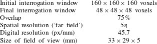
at the three locations studied. A summary of the spatial resolution and of the camera’s digital resolution is reported in table 1. (The digital resolution refers to how close the camera is to the object, whilst the spatial resolution is also a function of the final interrogation window of the PIV cross-correlation.)
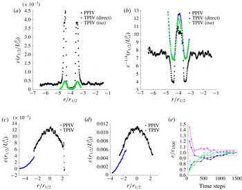
Comparison of the mean dissipation rate computed from the tomographic PIV of the present study and planar PIV (PPIV) from Breda & Buxton (Reference Breda and Buxton2018b
) at
 $x/D_{e}=2$
(a,b) and at
 $x/D_{e}=25$
(c–e). Estimates in which the dissipation rate is computed using an assumption of local isotropy from the TPIV data are also presented in (a,b) for direct comparison against the PPIV data. (b) Presents
 $\unicode[STIX]{x1D700}^{-1/4}$
to illustrate the computation of the Kolmogorov length scale
 $\unicode[STIX]{x1D702}=(\unicode[STIX]{x1D708}^{3}/\unicode[STIX]{x1D700})^{1/4}$
. (c,d) Are for the round and fractal jets respectively. (e) Convergence of the calculation for the mean dissipation rate from five data points chosen at random at
 $x/D_{e}=25$
.

Figure 4 gives an indication of the spatial resolution and convergence of the dissipation computation achieved in the present study. Comparison is made between the dissipation rate estimated from planar PIV (PPIV) in the study of Breda & Buxton (Reference Breda and Buxton2018b
) and the present tomographic PIV dataset. Figure 4(c,d) shows the round and fractal jets probed at the farthest downstream location of
 $x/D_{e}=25$
. The quoted worse-case spatial resolution of Breda & Buxton (Reference Breda and Buxton2018b
) at this downstream measurement station is
 $3.7\unicode[STIX]{x1D702}$
, which is sufficient to resolve the velocity gradients (e.g. Worth, Nickels & Swaminathan Reference Worth, Nickels and Swaminathan2010; Buxton et al.
Reference Buxton, Laizet and Ganapathisubramani2011). Since only planar data were available in this case the dissipation rate was estimated by assuming local isotropy from the PPIV data, whereas a direct computation, i.e.
 $\unicode[STIX]{x1D700}=2\unicode[STIX]{x1D708}\overline{\unicode[STIX]{x1D634}_{ij}\unicode[STIX]{x1D634}_{ij}}$
, was used for the TPIV data. It can clearly be seen that the TPIV slightly underestimates the dissipation rate in comparison with the PPIV as may be expected due to the coarser spatial resolution. However, the trends are extremely well captured and at least a portion of the difference between the two estimated dissipation profiles may be down to the assumption of local isotropy. This gives us confidence in our ability to draw meaningful conclusions relating to the VGT phenomenology in the present manuscript. (Note that the joint p.d.f. between
 $Q$
and
 $R$
extracted from along the irrotational boundary presented in figure 16 gives us further confidence that our spatial resolution is adequate to draw meaningful conclusions.)
Special note should be made here specifically about the spatial resolution at
 $x/D_{e}=2$
which is given as
 $11\unicode[STIX]{x1D702}$
in the worst case scenario. Clearly this is the coarsest of any of the measurement stations (in terms of turbulent length scales) and therefore the velocity gradients are likely to be an underestimate as a result of this spatial filtering. Indeed figures 4(a) and 4(b) show the dissipation rate
 $\unicode[STIX]{x1D700}$
and
 $\unicode[STIX]{x1D700}^{-1/4}$
which is the constituent part of the Kolmogorov length scale, at the
 $x/D_{e}=2$
measurement station which is clearly under-resolved. However, in terms of the Taylor length scale the resolution is always better than
 $0.3\unicode[STIX]{x1D706}_{f}$
. Buxton (Reference Buxton2015) showed that the tear-drop shape of the
 $Q$
–
 $R$
distribution relied upon resolving structures of characteristic length scale
 ${>}\unicode[STIX]{x1D706}_{f}$
in addition to the finest scales
 ${\sim}\unicode[STIX]{x1D702}$
. We finally note that our spatial resolution is thus always finer (including at
 $x/D_{e}=2$
) than the finest filter size (
 $\unicode[STIX]{x1D6E5}=0.4\unicode[STIX]{x1D706}$
) used in the large eddy simulation study of da Silva (Reference da Silva2009) to examine velocity-gradient phenomenology in the TNTI region of an axisymmetric jet. For this reason we are confident that we are able to draw at least qualitative conclusions from this measurement station even if we underestimate the VGT phenomenology quantitatively.
Figure 4(e) indicates the convergence of the calculation of the mean dissipation rate. Five data points were chosen at random from the dataset at
 $x/D_{e}=25$
and the mean dissipation rate was computed as a function of number of snapshots used in the calculation. It can be seen that the results lie well within the
 $\pm 5\,\%$
confidence intervals denoted by the dashed lines. We thus estimate the convergence of our dissipation rate estimate to be conservatively
 $\pm 3\,\%$
.
Processing details for planar and tomographic PIV. The worst case scenario for the spatial resolution is reported.

3 Properties of the TNTI
3.1 Detection of the TNTI
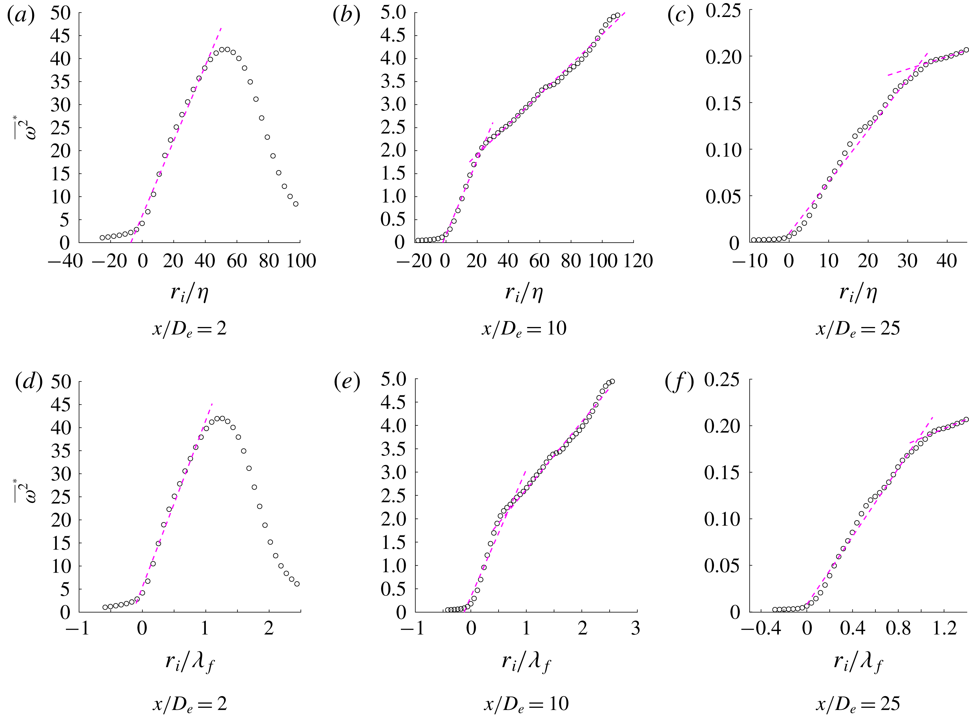
Value of
 $\overline{\unicode[STIX]{x1D714}^{2}}^{\ast }$
at various streamwise locations for the round jet, compensated by (a–c) the mean bulk
 $\unicode[STIX]{x1D702}$
and (d–f)
 $\unicode[STIX]{x1D706}_{f}$
. The changes of growth rate are shown with the dashed magenta lines.

The irrotational boundary between the turbulent and non-turbulent fluid (the outermost surface of the TNTI) was identified based on a vorticity-magnitude (twice enstrophy) threshold as has been used in previous studies (e.g. Bisset et al.
Reference Bisset, Hunt and Rogers2002; Holzner & Lüthi Reference Holzner and Lüthi2011). This threshold is necessarily non-zero due to experimental/numerical noise. Classically, in numerical studies the proportion of fluid identified as being in a turbulent state as a function of chosen vorticity-magnitude threshold yields a plateau region in which the turbulent proportion remains insensitive to small changes (da Silva et al.
Reference da Silva, Hunt, Eames and Westerweel2014). This is not possible for our experimental data due to the existence of (unavoidable) experimental noise and the weakly vortical, mild co-flow which was necessary to seed the background in order to avoid biasing the PIV experiments as (potentially unseeded) fluid is entrained into the jet with streamwise distance
 $x$
. As a result the threshold was chosen by use of an iterative procedure in which conditional statistics were produced as a function of distance from the irrotational boundary,
 $r_{i}$
. These statistics were then checked to ensure that they were insensitive to small changes in chosen threshold. These statistics included the conditional mean vorticity-magnitude jumps of figure 5, and ensuring that the joint p.d.f.s between
 $Q$
and
 $R$
extracted only from data points along the irrotational boundary contained minimal swirling states (see figure 16).
The threshold (discussed later in the paragraph) of the square root of vorticity magnitude was selected and the radial distance
 $r$
from the jet centre was converted into distance
 $r_{i}$
from the irrotational boundary, where
 $r_{i}=0$
corresponds to the irrotational boundary and positive
 $r_{i}$
is in the direction of the turbulent bulk. The conditional mean vorticity magnitude
 $\overline{\unicode[STIX]{x1D714}^{2}}^{\ast }$
(i.e. conditioned to the distance from
 $r_{i}=0$
) is premultiplied by the kinematic viscosity and dissipation rate
 $$\begin{eqnarray}\displaystyle & \displaystyle \overline{\unicode[STIX]{x1D714}^{2}}^{\ast }=\overline{\unicode[STIX]{x1D714}^{2}}\left(\frac{\unicode[STIX]{x1D708}}{\unicode[STIX]{x1D700}}\right), & \displaystyle\end{eqnarray}$$
and then plotted in figure 5(a). As shown, the threshold chosen captures the point where
 $\overline{\unicode[STIX]{x1D714}^{2}}^{\ast }$
sharply increases across the irrotational boundary, whilst for
 $r_{i}<0$
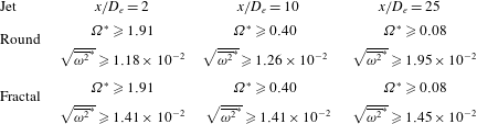
the vorticity magnitude is approximately zero. The threshold had to be adjusted for the three different streamwise locations studied, since the co-flow would slow down moving up vertically from the jet exit, showing as a consequence a reduced background vorticity. The values chosen were
 $\unicode[STIX]{x1D6FA}^{\ast }=(\overline{\unicode[STIX]{x1D714}^{2}})^{1/2}D_{e}/U_{e}\geqslant 1.91$
for
 $x/D_{e}=2$
,
 $\unicode[STIX]{x1D6FA}^{\ast }\geqslant 0.40$
for
 $x/D_{e}=10$
and
 $\unicode[STIX]{x1D6FA}^{\ast }\geqslant 0.08$
for
 $x/D_{e}=25$
. These thresholds were chosen based on the magnitude of the vorticity but when normalised by the kinematic viscosity and dissipation rate they are observed to be reasonably consistent between measurement stations, in particular for the fractal jet. This information is presented in table 2. A sensitivity study, which is not included for brevity, showed that all subsequent results were insensitive to small changes in threshold.
Normalised vorticity magnitude thresholds used to define the irrotational boundary.

In Bisset et al. (Reference Bisset, Hunt and Rogers2002), it was shown that for a fully developed turbulent wake
 $\overline{\unicode[STIX]{x1D714}^{2}}$
would be close to zero in the non-turbulent zone. It would then sharply increases across the TNTI and finally it would have a different and slower growth rate inside the wake. In figures 5(a)–5(c), two different behaviours can be identified as expected. There has been some debate as to the correct scaling of the TNTI thickness in ‘fully developed’ turbulent flows. Scaling of the TNTI thickness with
 $\unicode[STIX]{x1D706}_{f}$
has been widely reported in the literature (e.g. Westerweel et al.
Reference Westerweel, Fukushima, Pedersen and Hunt2009; da Silva & Taveira Reference da Silva and Taveira2010; Attili, Cristancho & Bisetti Reference Attili, Cristancho and Bisetti2014) although some doubt has now been cast on this for high Reynolds number flows (e.g. Watanabe et al.
Reference Watanabe, Sakai, Nagata, Ito and Hayase2015; Silva, Zecchetto & da Silva Reference Silva, Zecchetto and da Silva2018) who suggests that the correct scaling should be
 ${\sim}O(10)\unicode[STIX]{x1D702}$
. The purpose of this manuscript is not to examine the scaling of the TNTI thickness for developing flows, we do not compare against a broad range of Reynolds numbers, and so figures 5(a) to 5(c) depict
 $r_{i}$
compensated by
 $\unicode[STIX]{x1D702}$
and figures 5(d)–5(f) depict
 $r_{i}$
compensated by
 $\unicode[STIX]{x1D706}_{f}$
. Without determining a scaling it is merely reported that at
 $x/D_{e}=2$
, the TNTI has a thickness of
 ${\approx}1.2\unicode[STIX]{x1D706}_{f}$
, at
 $x/D_{e}=10$
of
 ${\approx}0.7\unicode[STIX]{x1D706}_{f}$
and of
 ${\approx}\unicode[STIX]{x1D706}_{f}$
at
 $x/D_{e}=25$
. Moreover, at
 $x/D_{e}=2$
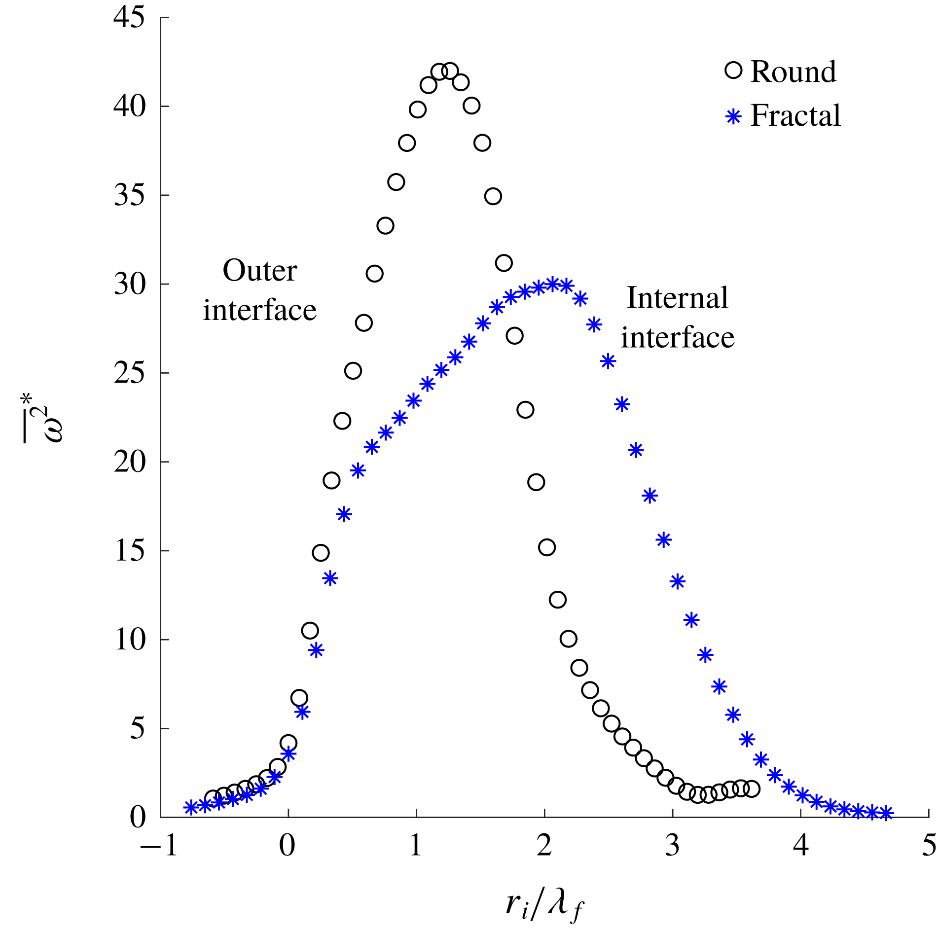
, the TNTI of the fractal jet appears to have a thickness of
 ${\approx}0.6\unicode[STIX]{x1D706}_{f}$
, which is almost half that of the round jet. This suggests that in the near field, the coherent structures present for the round jet alter the development of the TNTI, increasing the thickness of the outer TNTI, between the jet and the background fluid, whilst the TNTI between the jet and the core appears to have a comparable thickness between the round and fractal jets (figure 6). Note that at
 $x/D_{e}=2$
the flow should not be considered as a turbulent flow in the classical sense. Breda & Buxton (Reference Breda and Buxton2018a
) showed that for the round jet the there was a strong presence of azimuthally coherent vortical structures present at this location that were suppressed to a certain extent in the fractal jet. It is thus more instructive to think of the flow here as being transitional, nevertheless so as not to overburden the reader with additional terminology we refer to the interfacial region adjacent to the internal and external irrotational boundaries as TNTIs. Once the jet’s azimuthal shear layer coalesces and the core is absorbed, the TNTI’s thickness is initially less than a Taylor length scale but then evolves towards
 ${\approx}\unicode[STIX]{x1D706}_{f}$
once the turbulent flow is fully developed in the weakly self-similar region (
 $x/D_{e}=25$
). Further remarks are given in § 4.2.
Mean conditional interface for round and fractal jet at
 $x/D_{e}=2$
.

3.2 Tortuosity and radial locus of the TNTI
Breda & Buxton (Reference Breda and Buxton2018a
,Reference Breda and Buxton
b
) showed that a consequence of the fractal geometry, considered here, breaking up the coherent structures in the near field of the fractal jet (in comparison to the round jet) was a reduction of the entrainment and mixing rates. It is hypothesised, therefore, that the different coherent structures may affect the wrinkling of the interfaces and hence the surface area over which diffusion of vorticity may take place. The analysis focuses on two different types of TNTI. At
 $x/D_{e}=2$
, two interfaces are present: the outer interface (OTNTI), between the jet and the background flow, and the inner interface (ITNTI) (note that at
 $x/D_{e}=10$
and
 $x/D_{e}=25$
, the terminology TNTI refers to the outer interface of the jet since it is the only one present), between the laminar potential core and the turbulent part of the jet. The tortuosity is calculated for the ITNTI only, since the field of view was not big enough to always capture the complete OTNTI. This was estimated as a function of the averaged contorted interface length
 $L_{TNTI}$
across all time steps and the average radial distance
 $\overline{\hat{r}}$
of the TNTI from the jet centre (illustrated in figure 7),
 $$\begin{eqnarray}\displaystyle & \displaystyle tortuosity=\frac{L_{TNTI}}{2\unicode[STIX]{x03C0}\overline{\hat{r}}}. & \displaystyle\end{eqnarray}$$
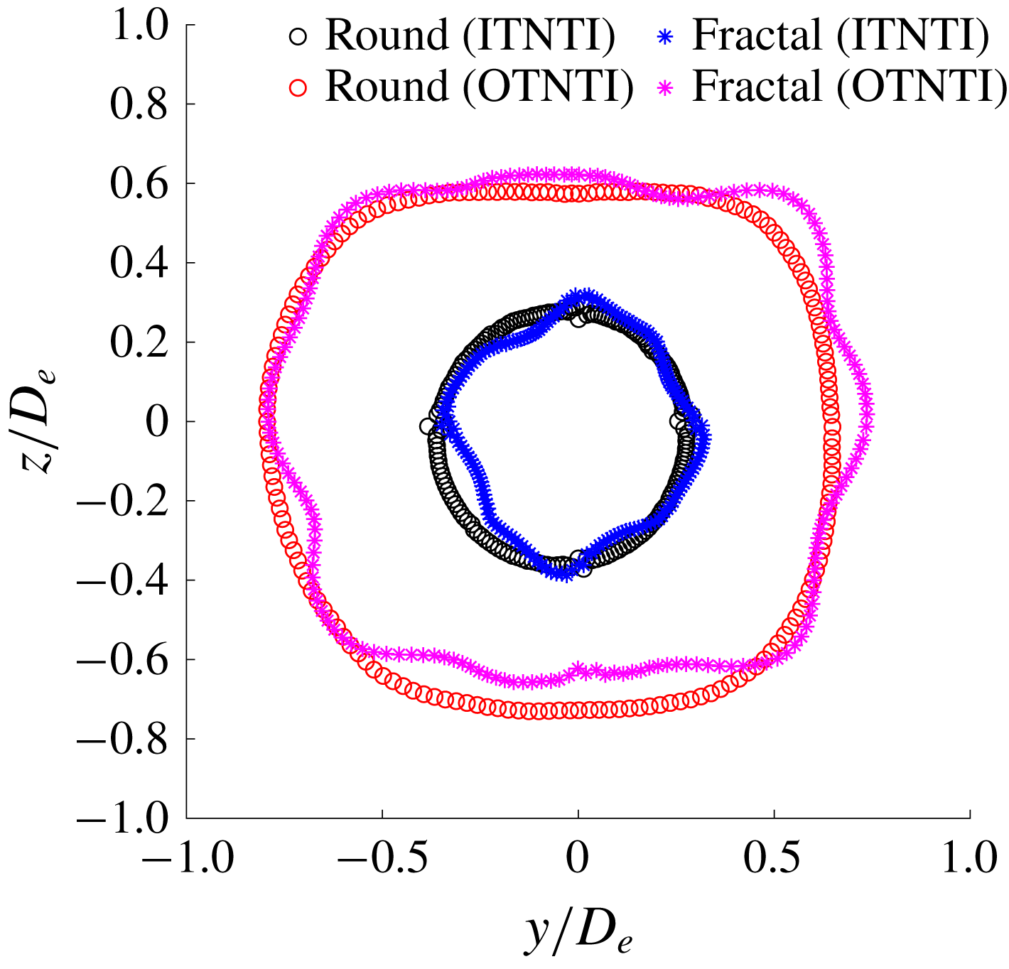
The interface length was directly calculated by following the Cartesian coordinates that defined the ITNTI. It is found that the round jet has a tortuosity of
 $1.49\pm 0.5\,\%$
, whilst for the fractal jet it is
 $1.40\pm 0.5\,\%$
. Hence, this hints that the break-up of the coherent structures may (slightly) reduce the wrinkling and the tortuosity of the ITNTI. In order to investigate this further, the probability density function of
 $\hat{r}$
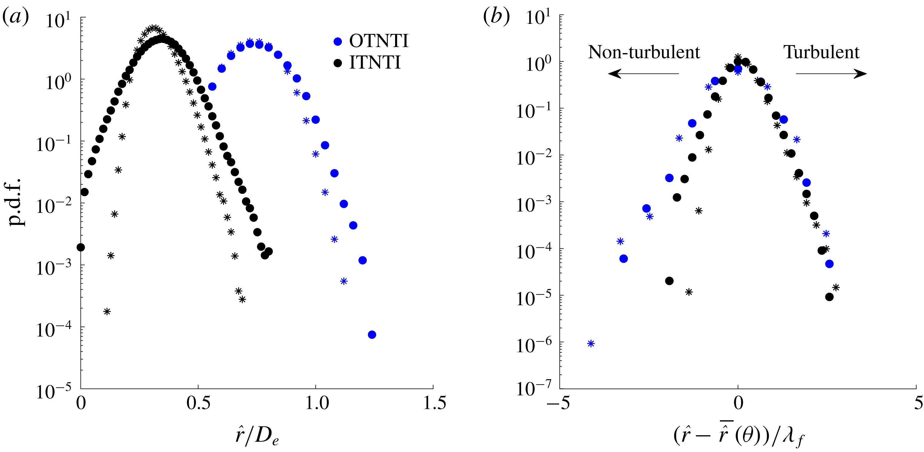
is examined. As shown in figure 8(a), the round jet has wider p.d.f.s at both ITNTI and OTNTI signifying more common large-scale excursions of the TNTIs. However, it is unclear if this is due to the suppression of the large-scale structures or simply due to the different exit geometry influencing the mean interface shape.
Value of
 $\overline{\hat{r}}(\unicode[STIX]{x1D703})$
for round and fractal jets at
 $x/D_{e}=2$
.

As shown in figure 7, both the ITNTI and the OTNTI of the fractal jet have a non-circular shape resembling the exit geometry, hence the radial fluctuations based on a single mean value for
 $\hat{r}$
may not be actually influenced by the exit geometry. Therefore, in order to evaluate the fluctuations of
 $\hat{r}$
, a different mean
 $\overline{\hat{r}}(\unicode[STIX]{x1D703})$
was calculated every
 $2^{\circ }$
, to account for the different shape of the two TNTIs. The p.d.f. of the fluctuations of
 $\hat{r}$
is examined in figure 8(b), where the abscissa has been re-ordered so that when it is positive the TNTI is moving towards the turbulent zone, whilst when negative towards the non-turbulent zone. It is found that the OTNTI and ITNTI of both jets have a comparable positive tail of the p.d.f., suggesting therefore that the movement towards the turbulent zone is not affected by the break-up of the coherent structures. On the negative side of the p.d.f., the OTNTI appears to have a larger tail compared to the ITNTI. Small differences are found on the ITNTI between the two jets, where the round jet has a larger negative tail indicating it is fluctuating more with respect to
 $\overline{\hat{r}}(\unicode[STIX]{x1D703})$
due to the influence of the large coherent structures. However, no appreciable differences are found on the negative side of the OTNTI of round and fractal jets, suggesting therefore it is insensitive to the state of the coherent structures. Note that the mean location of the OTNTI for the round jet is slightly non-circular. We ascribe this to slight asymmetries in the experimental configuration, for example due to a slightly non-uniform co-flow and the small wakes left by the four taut piano wires that were used to keep the central jet structure vertical.
(a) The p.d.f. of
 $\hat{r}$
for round (○) and fractal (*) jets. (b) The p.d.f. of fluctuations of the TNTI based on the angular mean radial distance (same legend applied). Here the abscissa has been oriented so that positive represents the turbulent zone, whilst negative represents non-turbulent areas (either in the jet core or in the quiescent background).

In Breda & Buxton (Reference Breda and Buxton2018a
), it was suggested that the break-up of the coherent structures produced a thinner shear layer that coalesced further downstream for the fractal jet, influencing the two-point correlations of the velocity fluctuations. This finding is here confirmed in terms of physical thickness, however it is shown that in terms of Taylor length scales the shear layer is in effect thicker for the fractal jet (figure 6). The ITNTI is also more corrugated in the presence of the strong coherent structures of the round jet, but this process is driven by large-scale excursions of the ITNTI – presumably driven by the coherent structures themselves. Interestingly, the primary difference between the two jets are the more common large excursions of the ITNTI into the potential core of the jet, as opposed to the excursions of the OTNTI towards the background fluid. Further downstream, comparable p.d.f.s are found between the two jets for
 $(\hat{r}-\overline{\hat{r}}(\unicode[STIX]{x1D703}))$
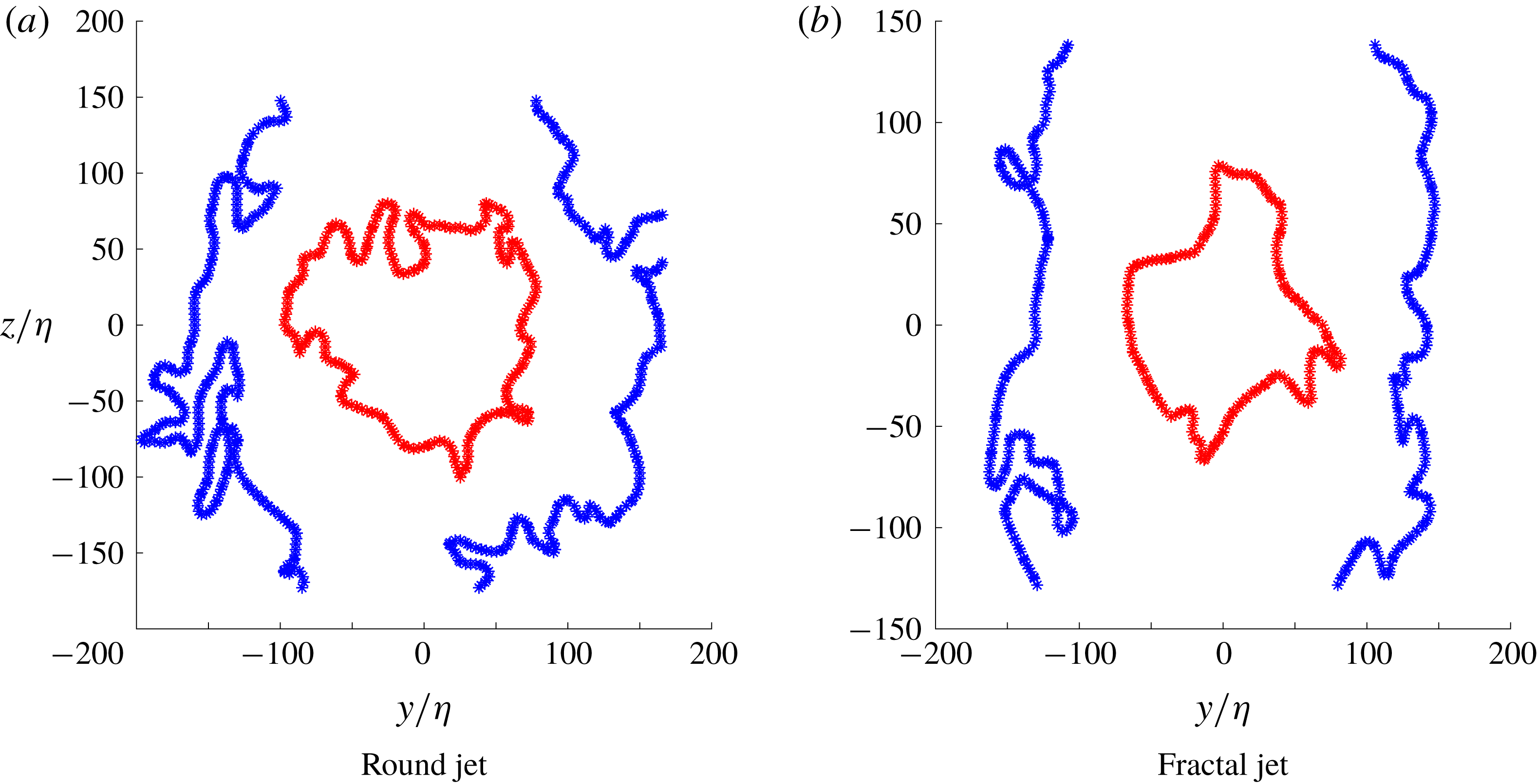
showing that this effect is confined to the near field. Note that the entrainment rates between the two jets also tended towards the same value further downstream, indicating that the modified entrainment rate in the near field may be a consequence of the modified ITNTI dynamics. Context to this finding is provided in figures 9(a) and 9(b) which show typical instantaneous TNTIs for the round and fractal jets respectively, scaled by the Kolmogorov length scale.
Instantaneous TNTIs, both inner and outer, with Cartesian spatial coordinates normalised by the Kolmogorov length scale for the round and fractal jets at
 $x/D_{e}=2$
.

3.3 Fractal dimension of the TNTI
Since the work of Sreenivasan & Meneveau (Reference Sreenivasan and Meneveau1986), it has been believed that the the area of a turbulent surface
 $S$
of a TNTI would follow a power law in the form
 $S\sim \unicode[STIX]{x1D6E5}^{2-D_{f}}$
, where
 $D_{f}$
is the (three-dimensional) fractal dimension and
 $\unicode[STIX]{x1D6E5}$
is the side length of a cube. As discussed by Mistry, Dawson & Kerstein (Reference Mistry, Dawson and Kerstein2018), invoking Reynolds’ similarity hypothesis and Kolmogorov scalings leads to a prediction of
 $D_{f}=2+1/3$
. Various computational and experimental works have attempted to verify this hypothesis, however strong limitations were posed by the spatial resolution and by the dimensions available (two-dimensional or three-dimensional). Therefore, rather than evaluating the area of the TNTI, the ‘fractality’ of its length was tested to check it would follow a power law. A popular method to verify this has been the ‘box counting’ technique (Mandelbrot Reference Mandelbrot1982; Sreenivasan, Ramshankar & Meneveau Reference Sreenivasan, Ramshankar and Meneveau1989; Mistry et al.
Reference Mistry, Philip, Dawson and Marusic2016; Zhou & Vassilicos Reference Zhou and Vassilicos2017). This technique consists in covering the field of view with squares of the same size and counting how many of them contains the TNTI.
Varying the box size
 $B_{s}$
and counting the number
 $N$
of boxes containing the TNTI, it should be found that there is a power law in the form
 $N\sim B_{s}^{m}$
. The exponent
 $m$
is related to the fractal dimension as
 $D_{f}=1-m$
. Therefore, if a Kolmogorov scaling were to be found it would be expected that
 $m=-4/3$
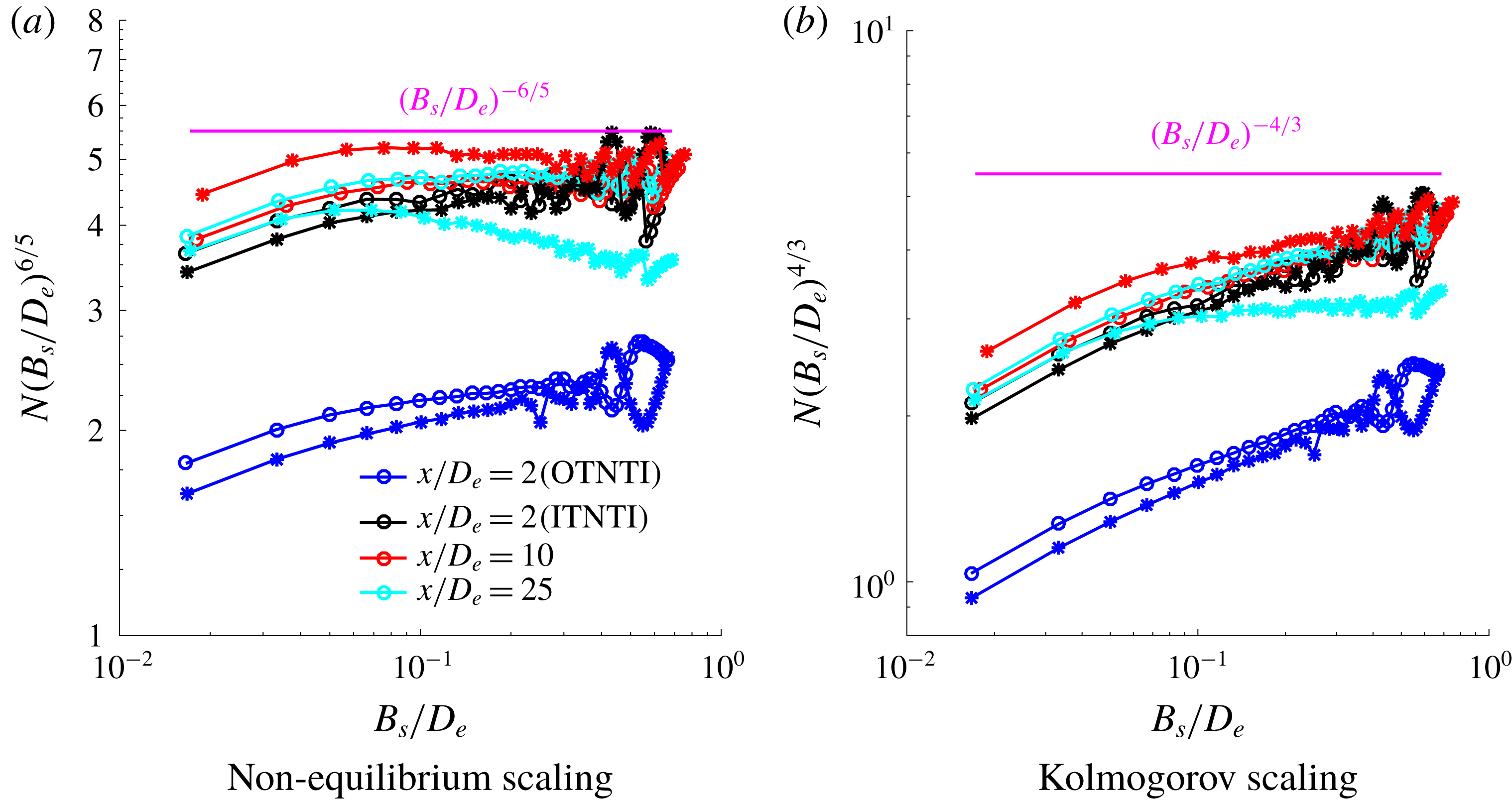
. The box-counting technique was applied to the present data at the various streamwise locations to probe the evolution of the TNTI further downstream. In order to test if they follow the Kolmogorov scaling, they are premultiplied so that if a specific scaling was followed, the data would lie on a straight horizontal line.
Box counting of different interfaces at various streamwise locations for round (○) and fractal (*) jets.

The data indicate that the TNTI follows a power law at all streamwise locations, however it does not seem to follow a Kolmogorov scaling. As shown in figure 10, the interfaces premultiplied by
 $(B_{s}/D_{e})^{6/5}$
in figure 10(a) appears to follow a
 $-6/5$
scaling rather than the
 $-4/3$
Kolmogorov scaling, as shown in figure 10(b). Only the fractal jet at
 $x/D_{e}=25$
appears to start approaching the Kolmogorov scaling, whilst the round jet does not. This may be linked to a different state of development of the TNTI at this stage since Breda & Buxton (Reference Breda and Buxton2018b
) showed that the number of eddies overturned, computed from integrating the eddy-turnover time and comparing it to the advection time scale required to advect distance
 $x$
, was substantially different between the round and fractal jets. However, more streamwise locations would need to be probed to confirm this and it should be noted that the p.d.f.s of
 $\hat{r}$
between the round and fractal jets did not show any discernible differences at this location.
This fractal dimension of
 $-6/5$
has been previously reported as the minimum value measured in jets and plumes by Lane-Serff (Reference Lane-Serff1993). The
 $-6/5$
scaling has also been previously discussed by Zhou & Vassilicos (Reference Zhou and Vassilicos2017), who completed three-dimensional (3-D) direct numerical simulations (DNS), looking at the TNTI in 2-D planes normal to the mean flow direction of an axisymmetric wake at various streamwise locations. Therefore, further streamwise locations are needed in order to unveil the transition from a
 $-6/5$
to a Kolmogorov scaling and which phenomena are determining it. The present findings differ from the results of Mistry et al. (Reference Mistry, Dawson and Kerstein2018), who investigated the scaling of the TNTI in the streamwise direction for an axisymmetric jet emitted by a round nozzle. The authors found that up to
 $x/D_{e}=5$
, the TNTI would have a 2-D fractal dimension lower than
 $4/3$
up to
 $x/D_{e}=5$
and then it would be approximately
 $4/3$
(hence a Kolmogorov scaling) from there up to
 $x/D_{e}=73$
(
 $x/D=65$
in the original work where
 $D$
is simply defined as the round jet diameter), where the jet was self-similar. The authors investigated the jet acquiring data in
 $r$
–
 $x$
planes rather than
 $r$
–
 $\unicode[STIX]{x1D703}$
planes as in the current work. It may be argued that it is more accurate to count the boxes in a
 $r$
–
 $\unicode[STIX]{x1D703}$
plane, as was also done by Zhou & Vassilicos (Reference Zhou and Vassilicos2017), at a specific streamwise location rather than counting them in the streamwise direction where the scaling may vary due to streamwise inhomogeneity.
4 Spatial evolution of the microscales of the jet
As outlined in § 1 one of the objectives of this manuscript is to investigate the spatial variation of the microscale flow physics in the near-interface region. This will reveal the adjustment of the small-scale properties of the turbulence from purely viscous-dominated flow physics in the viscous superlayer to the inertially dominated flow physics in the turbulent bulk portion of the flow. To do this, however, we must first examine the spatial evolution of the velocity gradients in the turbulent bulk of the jets, as the turbulence develops with streamwise distance
 $x$
.
4.1 State of the microscales of the jet
4.1.1 Spatial development of the j.p.d.f. of
$Q$
and
$R$


As discussed in § 1, the smallest scales of the flow are typically thought to be isotropic and statistically homogeneous and in ‘fully developed’ turbulence the joint probability density function between
 $Q$
and
 $R$
is found to have the so-called ‘tear-drop’ shape. However, Buxton et al. (Reference Buxton, Breda and Chen2017) found this shape also in the turbulence production region (the region in which turbulent kinetic energy is an increasing function of
 $x$
) for a wake generated by a high-aspect-ratio square cylinder, arguing that the tear-drop shaped j.p.d.f. may be a signature of turbulent flows in general. This contrasted previous findings from Gomes-Fernandes et al. (Reference Gomes-Fernandes, Ganapathisubramani and Vassilicos2014) who investigated the evolution of the microscales of grid-generated turbulence at close and intermediate distances from the grid. They found that the j.p.d.f. of
 $Q$
and
 $R$
would gradually acquire its tear-drop shape with increasing distance downstream, a finding also observed by Paul et al. (Reference Paul, Papadakis and Vassilicos2017). Hence it is now examined to determine whether the tear-drop develops in space or exists from the onset for axisymmetric jets. The region of the flow studied is the bulk of the turbulent flow, where
 $\unicode[STIX]{x1D6FA}^{\ast }>\mathit{threshold}$
as discussed in § 3.1. Despite the spatial resolution not being sufficient to resolve the Kolmogorov scale in the near field, Buxton (Reference Buxton2015) showed that a mix of inertial and dissipative scales is needed to recover the tear-drop shape. Hence, the current spatial resolution is sufficient to study some structural aspects of the small-scale behaviour of the flow.
The j.p.d.f. of
 $\mathit{Q}$
and
 $\mathit{R}$
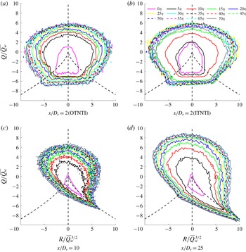
for the round and fractal jets. Isocontours range from
 $10^{-4}$
to
 $10^{0}$
. The regions of positive and negative
 $D$
(the discriminant of the velocity-gradient tensor) are separated by a black dashed line.

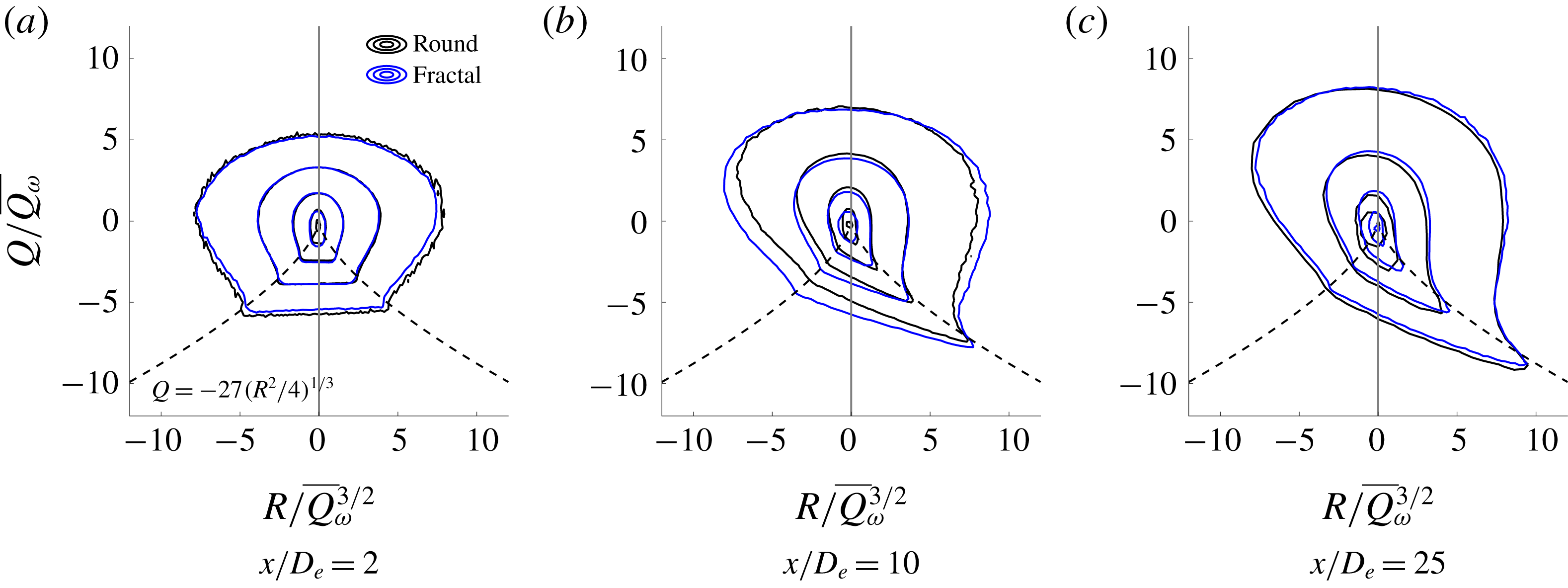
Figure 11 shows this spatial evolution of the j.p.d.f. of
 $Q$
and
 $R$
for both jets. At the farthest upstream station,
 $x/D_{e}=2$
where the disturbance/randomness has just been introduced, there is a close balance between events of
 $R>0$
and
 $R<0$
. We acknowledge that the spatial resolution, in terms of Kolmogorov length scale, is coarsest at this location meaning that it is possible that we have been unable to resolve a possible tear-drop shaped j.p.d.f. Nevertheless, this shape closely resembles the shape produced from the synthetic, Gaussian-distributed (i.e. less intermittent than ‘developed’ turbulence) data set produced in Cheng (Reference Cheng1996), Chertkov, Pumir & Shraiman (Reference Chertkov, Pumir and Shraiman1999) in which constraints on incompressibility and isotropy have been enforced. Given that we naturally expect the disturbance/randomness to originate at this spatial location the shape of the contours of figure 11(b)(a) agreeing with a Gaussian distribution of VGT states in which incompressibility/isotropy is enforced is somewhat reassuring that indeed these contours are physical rather than a result of lack of spatial resolution. Further, the potential effect of experimental noise at this station was investigated since, as discussed by Buxton et al. (Reference Buxton, Laizet and Ganapathisubramani2011), this j.p.d.f. can be highly susceptible to it. A further, more restrictive DCS was applied so that
 $|\unicode[STIX]{x2202}u_{i}/\unicode[STIX]{x2202}x_{i}|\leqslant 1~\text{s}^{-1}$
, however the same shaped j.p.d.f. was found, giving additional confidence that this result is physical and not a result of experimental noise. We observe that the
 $Q$
–
 $R$
contours begin to extend along the separatrix
 $4Q^{3}+27R^{2}=0$
, which is the discriminant of (1.2), or the so-called Vieillefosse tail (Vieillefosse Reference Vieillefosse1982) at the intermediate station
 $x/D_{e}=10$
. Note that at this location the turbulence intensity along the centreline of the jet is close to maximum and is decaying (Breda & Buxton Reference Breda and Buxton2018b
). At the farthest downstream location,
 $x/D_{e}=25$
, a recognisable tear-drop shape is found which is where the turbulence is the most ‘fully developed’ of any of the measurement stations (Breda & Buxton Reference Breda and Buxton2018b
).
In general, when a ‘classical’ tear-drop shape is present, in regions where strain dominates over rotation (
 $Q<0$
) strain production usually exceeds enstrophy production (
 $R>0$
), whilst in regions where rotation dominates (
 $Q>0$
) it is more likely that
 $R<0$
. At
 $x/D_{e}=2$
, the j.p.d.f. is approximately symmetrical and there is no trace of the so-called Viellefosse tail. Moreover, it is found that there is an approximately equal balance between events where strain production exceeds enstrophy production and vice versa. Therefore, it may be stated that at the start of the turbulence production region of a jet there is a balance between strain production and enstrophy production dominated events. This differs from the grid flow of Gomes-Fernandes et al. (Reference Gomes-Fernandes, Ganapathisubramani and Vassilicos2014), where the separated flow is immediately turbulent. However, similarly to grid-generated turbulence the tear-drop shape clearly evolves to a steady (developed) state with streamwise distance, via transient states originating from a Gaussian-like distribution. This is in contrast to a statistically two-dimensional bluff body wake in which the tear-drop shaped distribution is observed from immediately downstream of the body (Buxton et al.
Reference Buxton, Breda and Chen2017).
4.1.2 Evolution of enstrophy and strain production
We now consider some of the constituent terms of the invariant
 $R$
. Equation (1.4) shows that
 $R$
can be interpreted as a local departure from equilibrium between the inviscid strain-rate and enstrophy amplification terms. The analysis now focuses on the evolution of these terms,
 $-\unicode[STIX]{x1D634}_{ij}\unicode[STIX]{x1D634}_{jk}\unicode[STIX]{x1D634}_{ki}$
and
 $\unicode[STIX]{x1D714}_{i}\unicode[STIX]{x1D634}_{ij}\unicode[STIX]{x1D714}_{j}$
respectively.
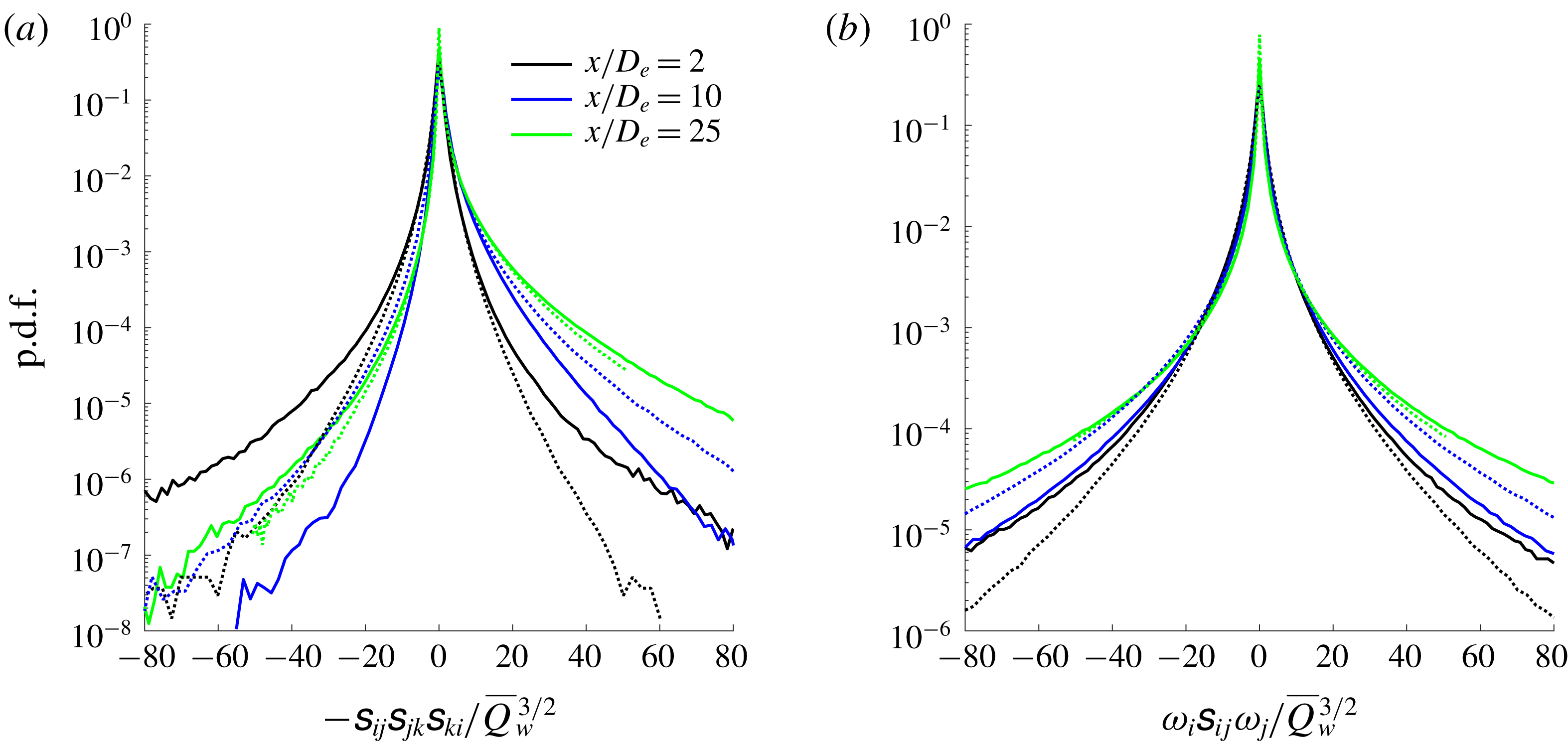
The p.d.f. of enstrophy and strain for the round jet (solid lines) and fractal jet (dotted lines).

In figure 12(a), the strain-rate production/destruction is analysed. The p.d.f.s at the three streamwise locations indicate that at
 $x/D_{e}=2$
strain destruction is favoured with respect to strain production. However, the flow then develops indicating a prevalence of strain production (
 $-\unicode[STIX]{x1D634}_{ij}\unicode[STIX]{x1D634}_{jk}\unicode[STIX]{x1D634}_{ki}$
) further downstream of the jet exit with an amplification of
 $-\unicode[STIX]{x1D634}_{ij}\unicode[STIX]{x1D634}_{jk}\unicode[STIX]{x1D634}_{ki}$
at the farthest location. The same behaviour was found by Gomes-Fernandes et al. (Reference Gomes-Fernandes, Ganapathisubramani and Vassilicos2014), who showed an increasing tendency for positive strain self-amplification (
 $-\unicode[STIX]{x1D634}_{ij}\unicode[STIX]{x1D634}_{jk}\unicode[STIX]{x1D634}_{ki}$
) moving further away from their space-filling fractal-square grid. We note that the strain destruction of the round jet appears to reach a minimum level at
 $x/D_{e}\approx 10$
before regaining its strength further downstream.
As discussed by Taylor (Reference Taylor1938), the inviscid vortex stretching term,
 $\unicode[STIX]{x1D714}_{i}\unicode[STIX]{x1D634}_{ij}\unicode[STIX]{x1D714}_{j}$
, is responsible for allowing the flow’s energy to be transferred inertially from the large to the small scales. On average
 $\langle \unicode[STIX]{x1D714}_{i}\unicode[STIX]{x1D634}_{ij}\unicode[STIX]{x1D714}_{j}\rangle >0$
, indicating therefore that vortex stretching is favoured over compression, and this has been verified in a wide range of flows (Tsinober, Kit & Dracos (Reference Tsinober, Kit and Dracos1992) amongst others). At
 $x/D_{e}=10$
and
 $x/D_{e}=25$
, the ensemble average of
 $\unicode[STIX]{x1D714}_{i}\unicode[STIX]{x1D634}_{ij}\unicode[STIX]{x1D714}_{j}$
is positive for both jets, in accordance with previous literature. This is also shown in figure 12(b), where the p.d.f. indicates a slight skewness towards the positive side. However, at
 $x/D_{e}=2$
 $\langle \unicode[STIX]{x1D714}_{i}\unicode[STIX]{x1D634}_{ij}\unicode[STIX]{x1D714}_{j}\rangle$
is negative for both jets, indicating a predominance of vortex compression over stretching.
4.1.3 Strain–vorticity coupling
As discussed by Betchov (Reference Betchov1956), the vortex stretching term can be rewritten as
 $\unicode[STIX]{x1D714}_{i}\unicode[STIX]{x1D634}_{ij}\unicode[STIX]{x1D714}_{j}=\unicode[STIX]{x1D714}^{2}s_{i}(\boldsymbol{e}_{\boldsymbol{i}}\boldsymbol{\cdot }\unicode[STIX]{x1D74E})^{2}$
, where
 $s_{i}$
are the eigenvalues of the strain-rate tensor,
 $\boldsymbol{e}_{\boldsymbol{i}}$
are the corresponding (unit) eigenvectors,
 $\unicode[STIX]{x1D74E}$
a unit vector indicating the direction of the vorticity vector and summation over index
 $i$
is implicit. Here,
 $s_{3}$
represents the compressive eigenvalue (always negative),
 $s_{1}$
the extensive one (always positive) and
 $s_{2}$
the intermediate one (either positive or negative). These eigenvalues can be ordered as
 $s_{1}\geqslant s_{2}\geqslant s_{3}$
and for an incompressible flow
 $\sum _{i=1}^{3}s_{i}=0$
.
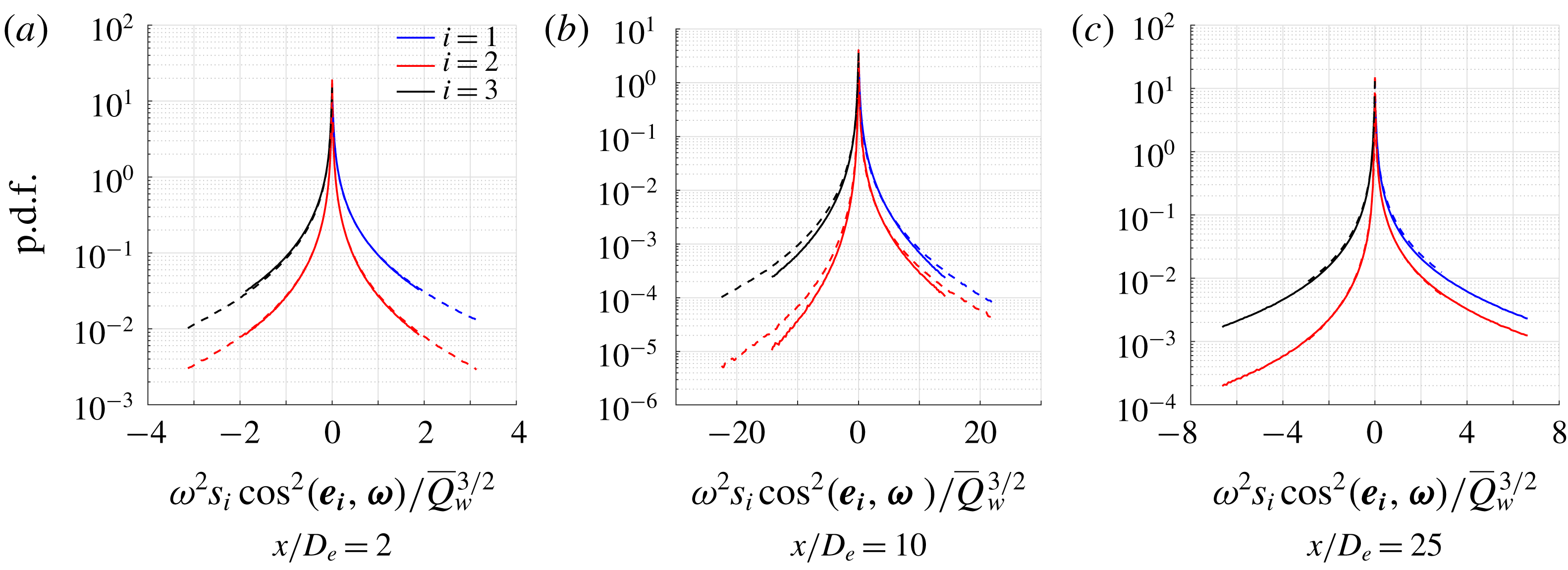
The p.d.f. of the spatial evolution of
 $\unicode[STIX]{x1D714}^{2}s_{i}\cos ^{2}(\boldsymbol{e}_{\boldsymbol{i}},\unicode[STIX]{x1D74E})$
for the round jet (solid lines) and the fractal jet (dashed lines).

As shown in figure 13(a), the symmetrical p.d.f. of
 $\unicode[STIX]{x1D714}_{i}\unicode[STIX]{x1D634}_{ij}\unicode[STIX]{x1D714}_{j}$
is confirmed at
 $x/D_{e}=2$
. At
 $x/D_{e}=10$
,
 $\unicode[STIX]{x1D714}^{2}s_{1}\cos ^{2}(\boldsymbol{e}_{\mathbf{1}},\unicode[STIX]{x1D74E})$
and
 $\unicode[STIX]{x1D714}^{2}s_{3}\cos ^{2}(\boldsymbol{e}_{\mathbf{3}},\unicode[STIX]{x1D74E})$
have an almost symmetrical p.d.f., whilst
 $\unicode[STIX]{x1D714}^{2}s_{2}\cos ^{2}(\boldsymbol{e}_{\mathbf{2}},\unicode[STIX]{x1D74E})$
has a clear skewness for vortex stretching which persists up to
 $x/D_{e}=25$
. At this station, the p.d.f.s of
 $\unicode[STIX]{x1D714}^{2}s_{1}\cos ^{2}(\boldsymbol{e}_{\mathbf{1}},\unicode[STIX]{x1D74E})$
and
 $\unicode[STIX]{x1D714}^{2}s_{3}\cos ^{2}(\boldsymbol{e}_{\mathbf{3}},\unicode[STIX]{x1D74E})$
are again similar, even though
 $\unicode[STIX]{x1D714}^{2}s_{3}\cos ^{2}(\boldsymbol{e}_{\mathbf{3}},\unicode[STIX]{x1D74E})$
appears to be slightly more intermittent, whilst the clear skewness of
 $\unicode[STIX]{x1D714}^{2}s_{2}\cos ^{2}(\boldsymbol{e}_{\mathbf{2}},\unicode[STIX]{x1D74E})$
points to the importance of the intermediate eigenvalue/vector
 $s_{2}/\boldsymbol{e}_{\mathbf{2}}$
in the process of vortex stretching. The findings in figure 13 show some similarities to the evolution of vortex stretching studied by Gomes-Fernandes et al. (Reference Gomes-Fernandes, Ganapathisubramani and Vassilicos2014). The authors found that, up to the turbulence production peak,
 $\unicode[STIX]{x1D714}^{2}s_{i}\cos ^{2}(\boldsymbol{e}_{\boldsymbol{i}},\unicode[STIX]{x1D74E})$
displayed symmetrical p.d.f.s, whilst in the decay region
 $\unicode[STIX]{x1D714}^{2}s_{2}\cos ^{2}(\boldsymbol{e}_{\mathbf{2}},\unicode[STIX]{x1D74E})$
would show a clear skewness towards positive values. However, differently from the present study, the authors found that
 $\unicode[STIX]{x1D714}^{2}s_{1}\cos ^{2}(\boldsymbol{e}_{\mathbf{1}},\unicode[STIX]{x1D74E})$
would have a wider p.d.f. compared to
 $\unicode[STIX]{x1D714}^{2}s_{3}\cos ^{2}(\boldsymbol{e}_{\mathbf{3}},\unicode[STIX]{x1D74E})$
, suggesting the behaviour of
 $\unicode[STIX]{x1D714}^{2}s_{i}\cos ^{2}(\boldsymbol{e}_{\boldsymbol{i}},\unicode[STIX]{x1D74E})$
might be intimately related to the particular flow studied.
We shall now attempt an explanation for the non-canonical behaviour of the velocity gradients at
 $x/D_{e}=2$
and why this canonical behaviour evolves towards
 $x/D_{e}=25$
. Clearly the coherent structures wane in influence with streamwise distance which is coupled to a departure from Gaussianity of the velocity gradients, which is necessary to enforce nonlinear behaviour such as
 $\langle \unicode[STIX]{x1D714}_{i}\unicode[STIX]{x1D634}_{ij}\unicode[STIX]{x1D714}_{j}\rangle >0$
. In addition, near the jet exit, the evolution of the strain field is somewhat constrained by the presence of the potential core, where the ITNTI and the OTNTI act like barriers to the development of the vortical structures. This idea is explored further in § 4.3. We may define a characteristic length scale separating the OTNTI and ITNTI as
 ${\mathcal{L}}_{\unicode[STIX]{x1D714}}=\hat{r}_{OTNTI}-\hat{r}_{ITNTI}$
, or simply the difference between the mean radius of the OTNTI and of the ITNTI. It is hypothesised that
 ${\mathcal{L}}_{\unicode[STIX]{x1D714}}$
may constrain the evolution of the turbulent structures if there is insufficient space to achieve a natural scale separation. Ishihara, Kaneda & Hunt (Reference Ishihara, Kaneda and Hunt2013) noted in their DNS work on homogeneous turbulence that thin layers of thickness
 $2.8\unicode[STIX]{x1D706}_{f}$
(
 $4\unicode[STIX]{x1D706}_{g}$
) exist, which consist of clusters of strong vortex tubes that contribute significantly to the mean dissipation rate. Elsinga et al. (Reference Elsinga, Ishihara, Goudar, Da Silva and Hunt2017) confirmed these findings for homogeneous turbulence (DNS) suggesting that the non-local strain width was
 $2.8\unicode[STIX]{x1D706}_{f}$
(
 $4\unicode[STIX]{x1D706}_{g}$
) and that the local strain scaled with
 $\unicode[STIX]{x1D702}$
. They were then able to attribute Reynolds number transitions in turbulence behaviour to those Reynolds numbers at which
 $\unicode[STIX]{x1D706}_{f}/\unicode[STIX]{x1D702}$
was sufficiently large to allow such structures to form. In the present study, it was found that
 $\overline{{\mathcal{L}}_{\unicode[STIX]{x1D714}}}\approx 1.8\unicode[STIX]{x1D706}_{f}$
for the round jet and
 $\overline{{\mathcal{L}}_{\unicode[STIX]{x1D714}}}\approx 2.4\unicode[STIX]{x1D706}_{f}$
for the fractal one at the
 $x/D_{e}=2$
measurement station.
Since
 $\overline{{\mathcal{L}}_{\unicode[STIX]{x1D714}}}$
is less than
 $2.8\unicode[STIX]{x1D706}_{f}$
for both jets, this may suggest that the physical space available is not sufficient for the non-local strain to develop. Hamlington, Schumacher & Dahm (Reference Hamlington, Schumacher and Dahm2008) showed that strain-rate and vorticity are linked by a nonlinear, non-local coupling. They showed that the non-local strain rate contributed significantly to the vortex stretching since the vorticity vector preferentially aligned with the background extensional strain rate, i.e.
 $\tilde{\boldsymbol{e}}_{\mathbf{1}}$
, with its correspondingly high magnitude eigenvalue
 $\tilde{s}_{1}$
, whereas it preferentially aligned with the intermediate local strain rate
 $\boldsymbol{e}_{\mathbf{2}}$
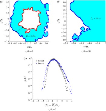
which has the lowest magnitude eigenvalue of any of the (local) principal strain rates. We thus postulate that the blocking effect of both TNTIs hinders vortex stretching through inhibiting the contribution of non-local strain. Further downstream, when the shear layer coalesces and the ITNTI is absorbed into the turbulent bulk, the strain has all the physical space necessary to evolve towards its (natural) non-local state. A schematic is shown in figures 14(a) and 14(b).
Example of turbulent length scales (a) constrained between the OTNTI and the ITNTI and (b) unconstrained (round jet). The turbulent area is shaded in light blue. (c) The p.d.f. of the fluctuations of
 ${\mathcal{L}}_{\unicode[STIX]{x1D714}}$
with respect to their mean
 $\overline{{\mathcal{L}}_{\unicode[STIX]{x1D714}}}$
.

The round and fractal jets have a comparable p.d.f. of the fluctuations of
 $\overline{{\mathcal{L}}_{\unicode[STIX]{x1D714}}}$
, where the positive side of the p.d.f. is wider than the negative one. In general, the p.d.f. of the fractal jet is only marginally wider than the one of the round jet as shown in figure 14(c), suggesting that the break-up of the coherent structures does not significantly alter the behaviour of
 ${\mathcal{L}}_{\unicode[STIX]{x1D714}}$
.
4.2 Small-scale evolution across the TNTI
We now focus on the spatial evolution of the state of the velocity gradients across the TNTI. This is done by extracting the joint p.d.f. between
 $Q$
and
 $R$
from specific spatial regions at a given distance from the irrotational boundary. The intervals chosen were
 $0{-}5\unicode[STIX]{x1D702}$
,
 $5{-}10\unicode[STIX]{x1D702}$
,
 $10{-}15\unicode[STIX]{x1D702}$
and so on up to
 $55{-}60\unicode[STIX]{x1D702}$
. An example is shown in figure 15. It is noted that due to the low spatial resolution the findings in the near field of the jet (
 $x/D_{e}=2$
) may appear filtered with respect to the stations further donwstream.
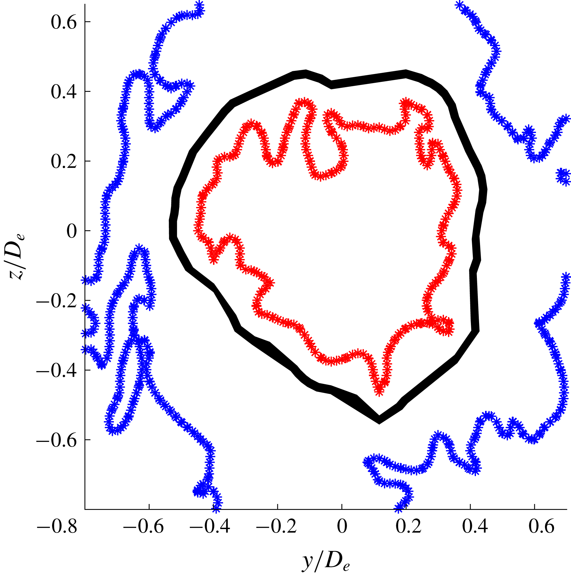
Example of an area probed between
 $15{-}20\unicode[STIX]{x1D702}$
at
 $x/D_{e}=2$
(black). The ITNTI is shown in red and the OTNTI in blue (Round jet).

The j.p.d.f. of
 $Q$
and
 $R$
, at a isocontour of
 $10^{-2}$
for the round jet (a comparable behaviour is found for the fractal jet as well).

The data presented in figure 16 suggest that at
 $r_{i}\approx \unicode[STIX]{x1D706}_{f}$
the contours become comparable between the evolving TNTI and the turbulent bulk region. For an incompressible flow (
 $P=-\unicode[STIX]{x1D622}_{ii}=0$
) the discriminant of (1.2) is given by
 $D=27/4R^{2}+Q^{3}$
and hence the curve
 $D=0$
, marked onto the figures, separates purely real roots for
 $D<0$
(straining motion only) from one real and a complex conjugate pair of roots for
 $D>0$
(swirling motion). Examining in detail the contours at the interface location, it is found that at
 $x/D_{e}=10$
and
 $x/D_{e}=25$
all the points are associated with
 $D<0$
, indicating purely straining motion. This is consistent with the original intuition of Corrsin & Kistler (Reference Corrsin and Kistler1954) and the DNS results of da Silva & Pereira (Reference da Silva and Pereira2008), who found the same behaviour at the irrotational boundary of a plane jet and provides further validation of our irrotational boundary detection threshold. The fact that this is not observed at
 $x/D_{e}=2$
is likely a result of the spatial filtering introduced as a consequence of the coarser spatial resolution (in terms of
 $\unicode[STIX]{x1D702}$
) at this measurement station coupled to the stronger background free stream turbulence (cf. the increased
 $\unicode[STIX]{x1D6FA}^{\ast }$
threshold at
 $x/D_{e}=2$
in table 2) resulting from the mild co-flow. The contribution of swirling dynamics, typically associated with vortex stretching/compression (Buxton & Ganapathisubramani Reference Buxton and Ganapathisubramani2010), increases with
 $r_{i}$
, i.e. within the turbulent sublayer of the TNTI. Note that the tear-drop shape begins to develop over a distance as small as
 $5\unicode[STIX]{x1D702}$
at
 $x/D_{e}=10$
and
 $x/D_{e}=25$
. This is similar to the finding of Watanabe et al. (Reference Watanabe, Jaulino, Taveira, da Silva, Nagata and Sakai2017) who showed that the tear-drop shape emerged after
 ${\approx}5.5\unicode[STIX]{x1D702}$
in their DNS of shear-free turbulence.
These findings suggest that the microscale properties vary inside the turbulent sublayer, whose thickness is comparable to
 $\unicode[STIX]{x1D706}_{f}$
. After that, the microscale properties remain the same as in the turbulent bulk at each streamwise location. Given that the present study considers two different jets, with differing contributions from large-scale coherent motions, at multiple streamwise measurement stations along the jets’ streamwise development this is a robust finding.
4.3 Consequences for the scaling of the TNTI thickness
Whilst the thickness of the TNTI has been reported to scale with
 $\unicode[STIX]{x1D706}_{f}$
(e.g. Bisset et al.
Reference Bisset, Hunt and Rogers2002; Westerweel et al.
Reference Westerweel, Fukushima, Pedersen and Hunt2005; Attili et al.
Reference Attili, Cristancho and Bisetti2014) or
 $\unicode[STIX]{x1D702}$
(Silva et al.
Reference Silva, Zecchetto and da Silva2018) this literature has not covered from which regions of the turbulent fluid these two length scales should be computed. Often, an average value of these two length scales has been calculated in the turbulent bulk or along the centreline of the flow. This is physically meaningful for a sufficiently ‘fully developed’ flow that the profiles of the relevant turbulent statistics have become self-similar. In such a flow the profile of the mean dissipation rate, a constituent in the computation of both
 $\unicode[STIX]{x1D706}_{f}$
and
 $\unicode[STIX]{x1D702}$
can be correctly scaled with just a single value of the dissipation, typically the centreline value
 $\unicode[STIX]{x1D700}_{0}$
. In developing, i.e. non-self-similar, flows such as the jets studied here this is not the case and it is not clear from where the mean dissipation rate should be extracted within the flow. It is usual to extract the value of
 $\unicode[STIX]{x1D706}_{f}$
or
 $\unicode[STIX]{x1D702}$
from within the turbulent bulk under the assumption that the turbulent behaviour of the TNTI is ‘slaved’ to the turbulent dynamics of the bulk flow (e.g. Attili et al.
Reference Attili, Cristancho and Bisetti2014).
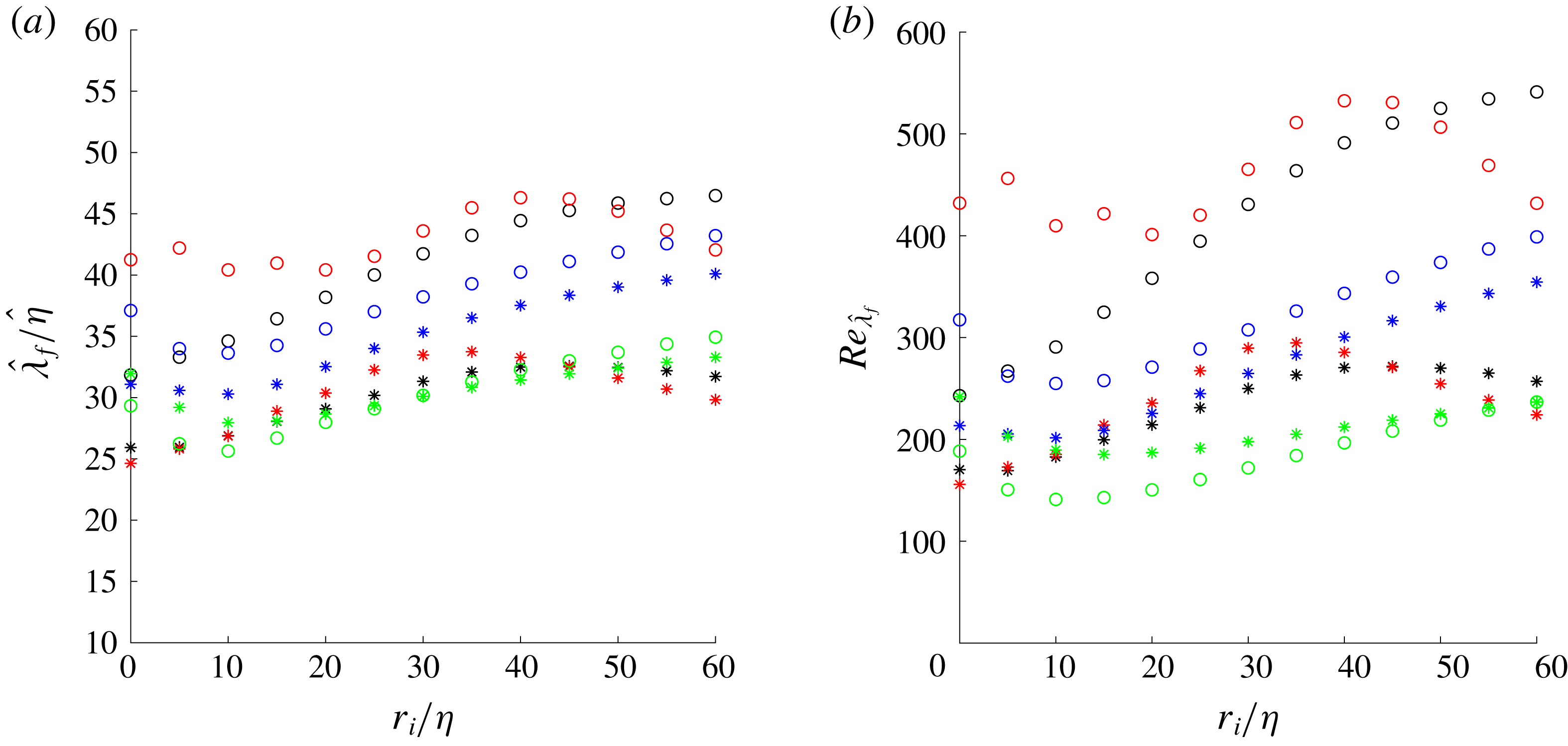
However, for shearless interfaces at least, doubt has been cast on this assumption. For example da Silva & Taveira (Reference da Silva and Taveira2010) argued that for shearless flows the TNTI consisted simply of the dissipative intense vorticity structures immediately adjacent to the irrotational boundary. More recently, Watanabe et al. (Reference Watanabe, Jaulino, Taveira, da Silva, Nagata and Sakai2017) made reasonable predictions of the conditional statistics across TNTIs using a model of a Burgers vortex placed within the turbulent sublayer of the TNTI of shear-free turbulence. In both cases the properties of the TNTI itself was shown to depend on the turbulence characteristics of the TNTI layer as well as the turbulent bulk and hence it is reasonable to probe the variability of turbulent length scales in this region. Figure 16 clearly shows that the state of the velocity gradients, and hence dissipation rate, is highly variable across the TNTI region. This opens the question as to whether a turbulent length scale computed from the turbulent bulk is relevant to a local scale computed within the TNTI region.
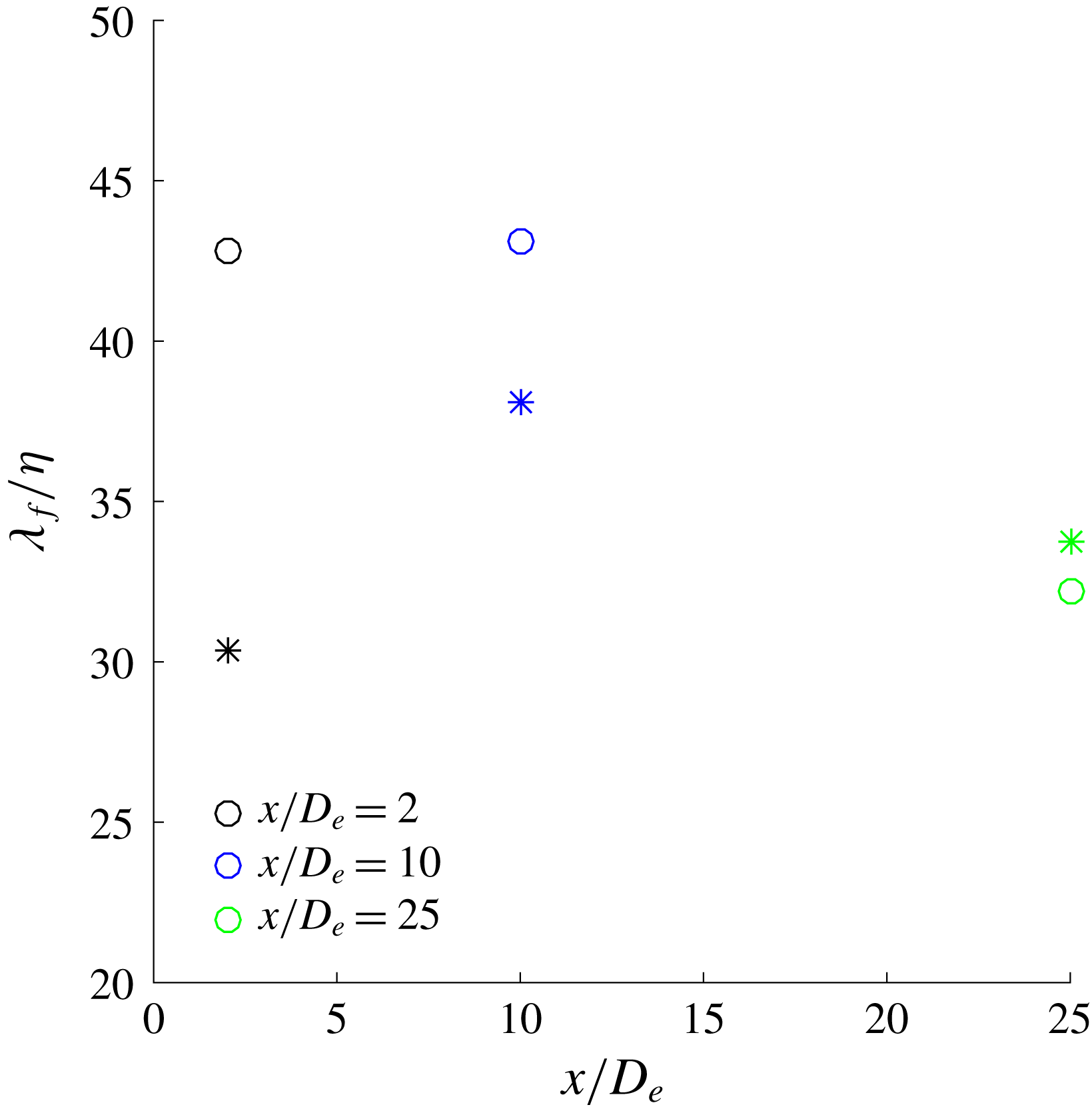
Evolution of the ratio between bulk
 $\unicode[STIX]{x1D706}_{f}$
and
 $\unicode[STIX]{x1D702}$
for round (○) and fractal jet (*).

Therefore, the evolution of
 $\unicode[STIX]{x1D702}$
and
 $\unicode[STIX]{x1D706}_{f}$
is examined ‘locally’, to verify how they change across the TNTI. To do so, the two local scales
 $\hat{\unicode[STIX]{x1D706}}_{f}$
and
 $\hat{\unicode[STIX]{x1D702}}$
are introduced. These are defined as
 $\hat{\unicode[STIX]{x1D702}}=(\unicode[STIX]{x1D708}^{3}/\hat{\unicode[STIX]{x1D700}})^{1/4}$
and
 $\hat{\unicode[STIX]{x1D706}}_{f}=(20\unicode[STIX]{x1D708}\hat{q}^{2}/\hat{\unicode[STIX]{x1D700}})^{1/2}$
where
 $\hat{\unicode[STIX]{x1D700}}$
is a local dissipation rate and
 $\hat{q}^{2}$
is a local turbulent kinetic energy computed from an ensemble situated at a particular distance from the TNTI. The local scales are computed at the irrotational boundary first and then in ‘slices’ of thickness
 $5\unicode[STIX]{x1D702}$
at various distances away from the TNTI in the same intervals as before:
 $0\unicode[STIX]{x1D702}$
,
 $0{-}5\unicode[STIX]{x1D702}$
,
 $5{-}10\unicode[STIX]{x1D702}$
,
 $10{-}15\unicode[STIX]{x1D702}$
and so on. Only the data points which are above the vorticity threshold previously discussed are included in the calculation. The findings are also evaluated in terms of the mean ratio between bulk
 $\unicode[STIX]{x1D706}_{f}$
and
 $\unicode[STIX]{x1D702}$
to verify if the local quantities vary across the TNTI only or not. The ratio for the two jets at various streamwise distances is shown in figure 17. This ratio represents scale separation in the flow and so the fact that both jets have an identical global Reynolds number of
 $Re_{G}=10^{4}$
but different
 $\unicode[STIX]{x1D706}_{f}/\unicode[STIX]{x1D702}$
ratios illustrates the effects that the fractal geometry has on the inertial/dissipative scales of the turbulence. Note that the difference reduces with streamwise distance as the turbulence develops which is consistent with our other findings.
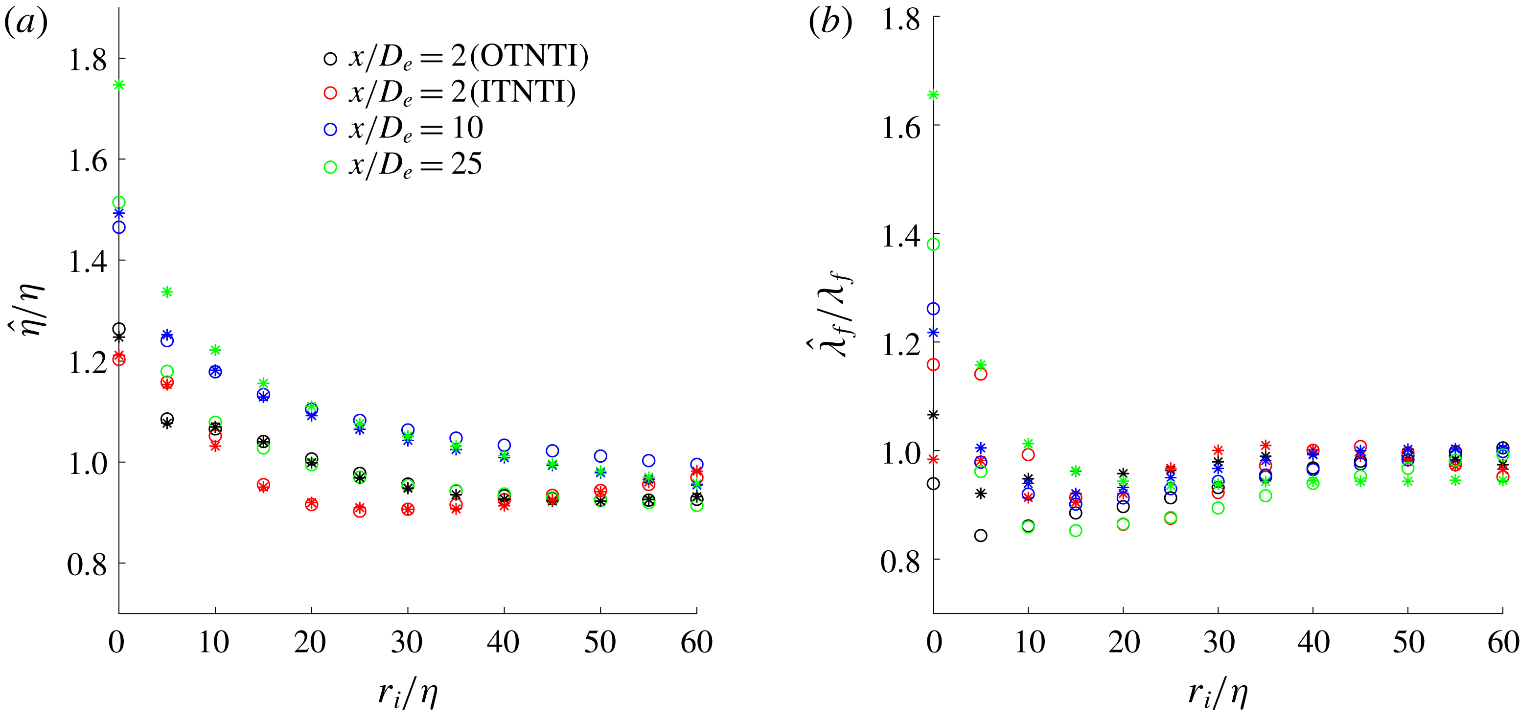
Evolution of (a) local Kolmogorov and of (b) local Taylor length scale for round (○) and fractal jets (*).

As shown in figure 18, both
 $\hat{\unicode[STIX]{x1D706}}_{f}$
and
 $\hat{\unicode[STIX]{x1D702}}$
vary significantly from the irrotational boundary towards the turbulent bulk. The greatest ratio between both length scales and their mean bulk value is at the interface. At the three streamwise locations,
 $\hat{\unicode[STIX]{x1D706}}_{f}$
appears to evolve up to a distance of
 $\unicode[STIX]{x1D706}_{f}$
away from the interface, after which it reaches a plateau. This would therefore suggest that the length scales evolve inside the TNTI of thickness
 $\unicode[STIX]{x1D706}_{f}$
, however they do not vary any more once the turbulent bulk is reached. The local
 $\hat{\unicode[STIX]{x1D702}}$
appears to take slightly longer to reach a plateau compared to
 $\hat{\unicode[STIX]{x1D706}}_{f}$
, even though the most rapid changes take place within a distance of
 $\unicode[STIX]{x1D706}_{f}$
again.
Examining the relationship between the local length scales, the ratio between these two scales changes based on the streamwise location and in general it increases from the irrotational boundary moving towards the turbulent bulk as shown in figure 19(a). At
 $r_{i}\approx 30{-}40\unicode[STIX]{x1D702}$
, this ratio decreases for the ITNTI and the OTNTI at
 $x/D_{e}=2$
, however this could be due to the fact that the points furthest away from one interface are approaching the other one. This is also reflected in figure 19(b), where the evolution of the local Taylor Reynolds number is examined. This is calculated as
 $Re_{\hat{\unicode[STIX]{x1D706}}_{f}}=\hat{u_{x}^{\prime }}\hat{\unicode[STIX]{x1D706}_{f}}/\unicode[STIX]{x1D708}$
, where
 $\hat{u_{x}^{\prime }}$
is the root-mean-square of the streamwise velocity fluctuations calculated in the same region as
 $\hat{\unicode[STIX]{x1D706}}_{f}$
. As shown,
 $Re_{\hat{\unicode[STIX]{x1D706}}_{f}}$
increases with increasing distance from the irrotational boundary, reflecting the behaviour of
 $\hat{\unicode[STIX]{x1D706}}_{f}/\hat{\unicode[STIX]{x1D702}}$
. This shows that there is a significant scale evolution from the TNTI moving towards the turbulent bulk and that choosing the mean bulk value to describe the state of a turbulent flow may not be representative.
Evolution of (a)
 $\hat{\unicode[STIX]{x1D706}}_{f}/\hat{\unicode[STIX]{x1D702}}$
and of (b)
 $Re_{\hat{\unicode[STIX]{x1D706}}_{f}}$
for round (○) and fractal jet (*). The legend is the same as figure 18.

Now a potential reason for such evolution is examined. The TNTI separates the non-turbulent from the turbulent fluid, acting like a ‘barrier’ between the two types of flow, as mentioned in § 4.1.3. This ‘blocking’ effect by the TNTI is similar to the concept of ‘shear sheltering’, discussed at length in Hunt & Durbin (Reference Hunt and Durbin1999), with the contrast that vortical motions are only present on one (the turbulent) side of the interface. The ‘blocking effect’ of the TNTI may be hypothesised to have a similar role to a wall in a turbulent boundary layer, which would lead to an increase of the small-scale anisotropy of the flow near the TNTI. Hence, this would affect the velocity gradients and as a consequence
 $\unicode[STIX]{x1D700}$
,
 $\unicode[STIX]{x1D706}_{f}$
and
 $\unicode[STIX]{x1D702}$
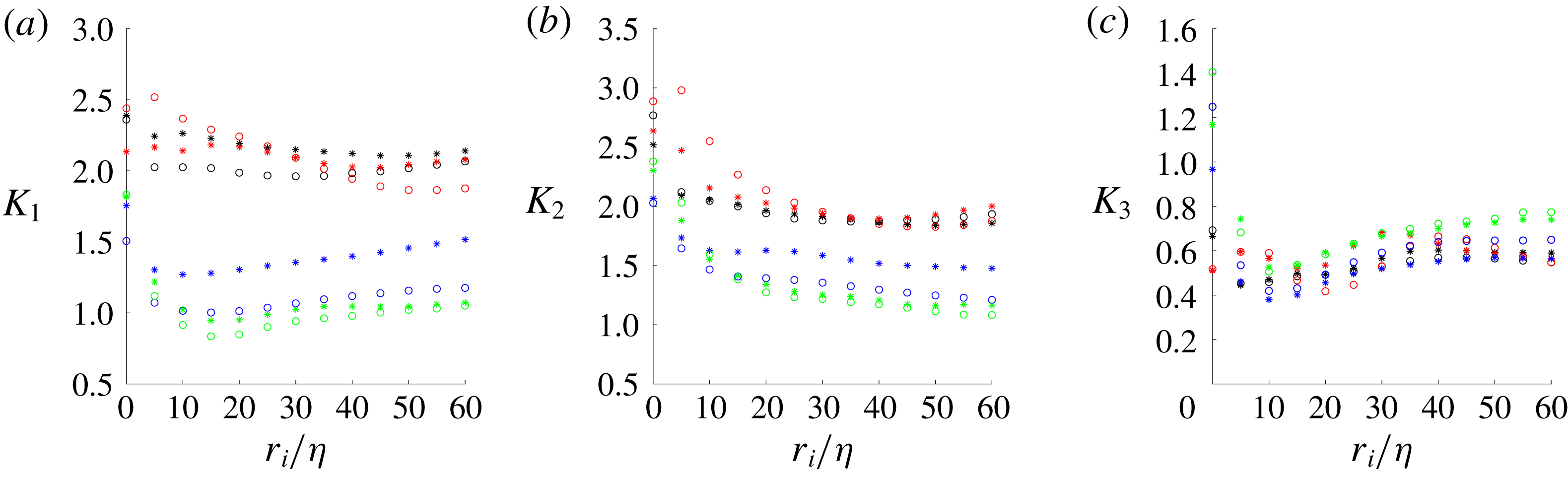
, since the interface-normal direction, similar to the wall-normal direction of a turbulent boundary layer, is highly anisotropic. In addition, the thin layer closest to the wall of a wall-bounded flow is dominated by viscous processes as is the outermost part of the TNTI. Bechlars & Sandberg (Reference Bechlars and Sandberg2017) showed that, for a compressible boundary layer, the wall-normal velocity gradient (and hence its anisotropy) would be dominant at the wall with respect to the other terms of the velocity-gradient tensor and it would decrease moving away from the viscous sublayer. We thus examine the state of the anisotropy in the TNTI through three ratios
 $K_{i}$
 $$\begin{eqnarray}\displaystyle & \displaystyle K_{1}=2\frac{\overline{(\unicode[STIX]{x2202}u_{x}/\unicode[STIX]{x2202}x)^{2}}}{\overline{(\unicode[STIX]{x2202}u_{r}/\unicode[STIX]{x2202}x)^{2}}},\quad K_{2}=2\frac{\overline{(\unicode[STIX]{x2202}u_{x}/\unicode[STIX]{x2202}x)^{2}}}{\overline{(\unicode[STIX]{x2202}u_{\unicode[STIX]{x1D703}}/\unicode[STIX]{x2202}x)^{2}}},\quad K_{3}=2\frac{\overline{(\unicode[STIX]{x2202}u_{x}/\unicode[STIX]{x2202}x)^{2}}}{\overline{(\unicode[STIX]{x2202}u_{x}/\unicode[STIX]{x2202}r)^{2}}}, & \displaystyle\end{eqnarray}$$
to verify how the velocity gradients evolve from the irrotational boundary towards the turbulent bulk.
As shown in figure 20, the anisotropy is the greatest at the irrotational boundary for all streamwise locations and for all the three
 $K_{i}$
. The trends of
 $K_{1}$
and
 $K_{2}$
appear to decrease moving further downstream, as expected due to the reduced influence of the coherent structures, however an isotropic state where
 $K_{i}=1$
is not yet reached for all ratios. Moreover, at
 $x/D_{e}=2$
the flow is constrained by the presence of two TNTIs, which may not leave enough space to the flow to recover any ‘bulk’ isotropy. In general a plateau or a constant trend is found after a distance of
 $\unicode[STIX]{x1D706}_{f}$
. It appears that these anisotropy ratios vary mainly inside the TNTI as
 $\hat{\unicode[STIX]{x1D706}}_{f}$
and
 $\hat{\unicode[STIX]{x1D702}}$
. Therefore, this suggests that the local quantities are strongly influenced by the anisotropy of the flow especially inside the TNTI.
Evolution of (a)
 $K_{1}$
, (b)
 $K_{2}$
and (c)
 $K_{3}$
for round (○) and fractal jets (*). The legend is the same as figure 18.

5 Discussion and conclusions
It was found that the break-up of the coherent structures by the fractal orifice affects the tortuosity of the ITNTI and also reduces the thickness of the OTNTI in the near field. The excursions of the TNTI are similar for both jets when the interface moves towards the turbulent side whilst they vary if the interface moves towards the non-turbulent side. Whilst the excursions of the OTNTI were comparable between the two jets it was shown that the round jet, with a stronger contribution from the coherent structures, sees more common large-scale excursions of the ITNTI into the potential core. This leads to a slightly more tortuous ITNTI for the round jet, with a presumably correspondingly greater surface area over which entrainment via nibbling may take place. It thus seems that the difference in entrainment rates in the near fields of both jets reported in Breda & Buxton (Reference Breda and Buxton2018b
) may be a result of both enhanced engulfment (large-scale excursions of the TNTI are likely to promote this) and enhanced nibbling through a more contorted interface. Using a box-counting technique, it was verified that the TNTI follows a scaling of
 $N\sim B_{s}^{-6/5}$
in the regions studied, whilst only the fractal jet appears to start approaching the Kolmogorov scaling of
 $N\sim B_{s}^{-4/3}$
in the furthest downstream measurement station. This perhaps suggests that there is a difference between examining the fractal dimension of the TNTI in a streamwise – radial plane as opposed to an azimuthal – radial plane.
We report here the spatial development of the
 $Q$
–
 $R$
j.p.d.f. for an axisymmetric turbulent jet for the first time. Its spatial development, like that for grid-generated turbulence in Gomes-Fernandes et al. (Reference Gomes-Fernandes, Ganapathisubramani and Vassilicos2014), contrasts to the tear-drop shaped distribution being observed throughout the near-wake region of a statistically two-dimensional bluff body wake in Buxton et al. (Reference Buxton, Breda and Chen2017). An analysis of the microstructure of the jets indicated that, in the near field, turbulence is constrained between the ITNTI and of the OTNTI. This inhibits the background non-local strain field, which occurs concurrently to a suppression of the inviscid vortex stretching term. Comparing the present work with that of Gomes-Fernandes et al. (Reference Gomes-Fernandes, Ganapathisubramani and Vassilicos2014), it is confirmed that the
 $Q$
–
 $R$
j.p.d.f. develops with streamwise distance from the jet exit. Other similarities are represented by the initial balance between the inviscid production and destruction of strain rate and enstrophy. However, some differences are present in the near field, where for a round jet there are two TNTIs and the flow is initially not fully turbulent. In fact, the symmetrical j.p.d.f. of
 $Q$
–
 $R$
at
 $x/D_{e}=2$
was not found by Gomes-Fernandes et al. (Reference Gomes-Fernandes, Ganapathisubramani and Vassilicos2014).
By comparing the round and fractal jets a comparison was also made between two flows with identical global Reynolds numbers but different coherent structures embedded into the flow, and hence initial conditions. The ratio
 $\unicode[STIX]{x1D706}_{f}/\unicode[STIX]{x1D702}$
is indicative of the range of scales present within the flow, and hence the local turbulent Reynolds number. Despite the different initial conditions, and a different range of length scales present i.e. different
 $\unicode[STIX]{x1D706}_{f}/\unicode[STIX]{x1D702}$
ratios, the velocity-gradient phenomenology of the round and fractal jets was extremely similar at the intermediate measurement station
 $x/D_{e}=10$
. This highlights the short ‘memory’ that the microscales of the flow have of their initial conditions and the robustness of the
 $Q$
–
 $R$
statistical distribution.
The analysis then moved towards understanding how the velocity gradients varied through the TNTI of nominally axisymmetric jets, into the turbulent bulk. It was found that in most cases the contours of the joint p.d.f.s between the invariants
 $Q$
and
 $R$
start collapsing after a distance of
 $\unicode[STIX]{x1D706}_{f}$
away from the irrotational boundary, suggesting that the microscale structure of the jet evolves across the interface before becoming comparable to the turbulent bulk. This variation of the behaviour of the velocity-gradient invariants in the interface region is coupled to a sharp increase in the small-scale anisotropy. This behaviour of the velocity gradients results in a substantial change of the local Taylor and Kolmogorov length scales,
 $\hat{\unicode[STIX]{x1D706}}_{f}$
and
 $\hat{\unicode[STIX]{x1D702}}$
respectively, with distance from the irrotational boundary. It appears that a distance of
 $\unicode[STIX]{x1D706}_{f}$
is necessary for the length scales to have a comparable value spatially. The evolution of turbulent properties also takes place across a distance of
 $\unicode[STIX]{x1D706}_{f}$
for both jets, indicating that the initial conditions may only impact large-scale phenomena directly, whilst the fine structure of the flow remains relatively unaltered. This does not, however, discount an indirect effect on small-scale processes such as nibbling through an increase in the surface area of the TNTI over which it may take place.
Acknowledgements
The authors gratefully acknowledge EPSRC for funding through EPSRC grant no. EP/L023520/1.