Related literature

The question we analyze—when do local politicians support copartisan candidates to national office—concerns hierarchical relations among politicians within the same party. Various literatures analyze similar concerns. An extensive literature on voter mobilization has inspected the effects of local campaigning and canvassing on the electoral fortunes of political parties, especially through the promotion of turnout (Merriam and Gosnell Reference Merriam and Gosnell1924; Gosnell Reference Gosnell1937; Patterson and Caldeira Reference Patterson and Caldeira1983; Caldeira et al. Reference Caldeira, Clausen and Patterson1990; Green and Gerber Reference Green and Gerber2004). However, this literature is not concerned with whether the local party organization will choose to boost the party’s vote share (it will!), but rather with which local politicians should be awarded resources to aid mobilization efforts on behalf of the party (e.g., Holbrook and McClurg Reference Holbrook and McClurg2005).

The literature on coattail effects has also recognized that copartisan candidates in different electoral arenas benefit from each others’ efforts (Ferejohn Reference Ferejohn1986; Samuels Reference Samuels2000; Carey Reference Carey2003; Magar Reference Magar2012; Ames Reference Ames1994). These effects, however, result from externalities of the effort that candidates make to secure their own victories. The idea is that a local candidate that manages to turn out a large number of sympathizers to vote for her might end up bolstering the vote share of copartisan candidates elected concurrently to other posts. If voters mostly vote straight tickets, coattails obtain even when the more recognizable candidate makes no explicit attempt to improve the vote share of copartisan candidates.

A growing literature on multi-level parties explores how local and national politicians interact under various institutional arrangements (Koelble Reference Koelble1996; Van Houten Reference Van Houten2009), how a discernible “local vote” might emerge as a consequence of certain national-level determinants (Morgenstern and Swindle Reference Morgenstern and Swindle2005), how coordination of electoral strategies among local and national politicians shapes national party systems (Caramani Reference Caramani2004; Gibson Reference Gibson2012), and how national elites interact with local machines in clientelistic party systems (e.g., Weitz-Shapiro Reference Weitz-Shapiro2012; Albertus Reference Albertus2013; Stokes et al. Reference Stokes, Dunning, Nazareno and Brusco2013). These works focus on the micro-foundations of solidarity among copartisans and are close to our contention that within-party cooperation is not self-enforcing.

However, few have attempted to formalize the agency dilemmas that we highlight in this paper. Zudenkova (Reference Zudenkova2011) mentions the possibility that copartisan politicians may free-ride on each others’ campaigning efforts, but this is in a model of coattails that arise because candidates care about their copartisans’ performance and voters evaluate copartisan candidates jointly. Shachar and Nalebuff (Reference Shachar and Nalebuff1999) suggest that US governors have an incentive to mobilize in favor of copartisan presidential candidates when they anticipate that their state will be pivotal in the electoral college. Kemahlıoğlu (Reference Kemahlıoğlu2012) studies tensions between local and national politicians that obtain as the former build support networks across localities: national politicians have an incentive to fund the creation of these networks—they are helpful to mobilize voters—but are also wary that local politicians can use them to challenge their leadership. Stokes et al. (Reference Stokes, Dunning, Nazareno and Brusco2013) model clientelistic brokers as opportunistic agents with private information who recruit partisan rather than swing voters in order to signal their mobilization capacity—thus complicating their party’s effort to target voters efficiently. Rundlett and Svolik (Reference Rundlett and Svolik2016) argue that local agents do not engage in electoral fraud on behalf of a hegemonic party if the chance of losing the election is too large—they can get caught and be punished by the victorious opposition—; however, if the chance of winning is high enough, they participate willingly to increase the chance of a reward. Thus, fraud is either over- or under-supplied. This result obtains because they model the cost of fraud as conditional on the election outcome, while we treat the cost of exerting effort as fixed. Last, Persico et al. (Reference Persico, Rodríguez Pueblita and Silverman2011) and Benton (Reference Benton2007) build models of intra-party strife in which within-party factions appear when politicians compete to obtain patronage or local public goods for their districts. In contrast, our contribution illuminates some of the mechanisms that prevent local politicians from supporting copartisans even when factionalism is not a relevant concern.

A theory of local mobilization in multi-level parties

We develop a model in which politicians at different government levels—“mayors” in cities and “governors” in states—act as agents of a copartisan candidate who is running for a congressional seat. We seek to understand the incentives that push local politicians to exert effort on behalf of the national candidate. We focus on the strategic interaction between one governor (G) and up to three copartisan mayors, which is the easiest way to capture variation in the proportion of mayors in a district that are copartisans of the governor.

This political geography captures conditions typical of many political systems. Mayors govern cities that are nested within electoral districts. Governors govern states that comprise several electoral districts, though for simplicity we assume that state and district are coterminous. We model mayors as politicians that court gubernatorial support to further their careers. Gubernatorial support appears as a decision to reward the mayor for a job well done, and broadly captures any kind of support that aids the mayor’s career, such as endorsement for a re-election run, promotion within the party ranks, or nomination for a candidacy to higher office. Voters appear indirectly in the model through a parameter that captures the party’s “normal vote” in the district. Our goal is to study the behavior of local politicians in a context in which they have the means to benefit their copartisans but lack an incentive to mobilize voters because their own reelection is not at stake. For this reason, we assume that local and national elections are not concurrent.Footnote ³

Governors and mayors can increase the probability that their copartisan candidate will carry the district by mobilizing voters, which requires effort. We treat effort exerted by mayors and governor as additive, so that the probability that the national candidate will carry a district when all agents exert effort is strictly larger than when only some do.Footnote ⁴ Players have utilities defined over effort and reward. Specifically, mayors obtain reward r>0 if promoted by the governor, which can only occur if the party wins the district. The cost of exerting effort depends on a mayor’s type. With probability τ∈(0,1), a mayor is of good type and pays no cost for exerting effort (f _g (e)=0), while bad-type mayors incur a cost from effort (f _b (e)=f>0). The governor is interested in promoting good mayors because these are capable of helping the party in the future. To capture this incentive, G receives a payoff of R=1 for promoting a good type, and R=0 otherwise.

To decide whom to promote, the governor can invest effort in monitoring mayoral behavior. Monitoring detracts from campaigning directly on behalf of the party’s candidate, introducing a sharp trade-off in the governor’s actions. At the beginning of the game, the governor decides between two options that we model as mutually exclusive for the sake of simplicity: to campaign on behalf of her party (c) or to monitor the behavior of mayors (m). Specifically, G must choose between {m=1, c=0} with cost g>0; {m=0, c=1} with cost k>0; or {m=c=0}, which is costless. Admittedly, real-life governors might split effort between campaigning and monitoring, or may campaign once monitoring reveals information about a mayor’s behavior. However, gubernatorial effort is limited, and the assumption that effort can be deployed either to monitor or to campaign puts in sharp relief the consequences of adopting either action without changing the strategic environment. Through monitoring, G can ascertain whether a mayor exerted effort or not. For simplicity, we assume that if the governor chooses to monitor, she picks a copartisan mayor at randomFootnote ⁵ and receives a perfectly reliable signal of whether the mayor exerted effort, though not of the mayor’s type. At the end of the game, the governor chooses to reward up to one copartisan mayor, though she may also decide not to reward anyone.

The outcome of interest is the probability that the party’s candidate will win the district, which depends on the effort of the governor and mayors (c and e, respectively), the district’s proclivity to vote for the opposition (v∈[−1,1]), and a pro-opposition shock ε with known uniform distribution along the $$[{\minus}{1 \over {2\psi }},{1 \over {2\psi }}]$$ interval, with ψ∈(0,1/5].Footnote ⁶ With these assumptions in place, the probability of victory in the district is:

$$\Pr ({\rm Win})\,\equiv\,\Pr ({\varepsilon} \leq \mathop{\overbrace{{I[c]s}}}^{{\scriptstyle {\rm Governor's} \atop {\scriptstyle {\rm campaigning} \atop \scriptstyle {\rm effort}}} }{\plus} \mathop{\overbrace{{\Sigma _{{i\in{\cal I}}} I[e_{i} ]\left( {{{1{\minus}s} \over 3}} \right)}}}^{{\scriptstyle {\rm Copartisan\; mayors'} \atop \scriptstyle {\rm campaigning\; effort}} } {\minus} \mathop{\overbrace{{\Sigma _{{o\in{\cal O}}} I[e_{o} ]\left( {{{1{\minus}s} \over 3}} \right)}}}^{{\scriptstyle {\rm Opposition\; mayors'} \atop \scriptstyle {\rm campaigning\; effort}} } {\minus} v)$$

$${\equals}{\int}_{{\minus}{1 \over {2\psi }}}^{I[c]s{\plus}\Sigma _{{i\in{\cal I}}} I[e_{i} ]{1 \over 3}(1{\minus}s){\minus}\Sigma _{{o\in{\cal O}}} I[e_{o} ]{1 \over 3}(1{\minus}s){\minus}v} h({\varepsilon})d{\varepsilon}$$

(1) $$\Pr ({\rm Win}){\equals}{1 \over 2}{\plus}\psi (I[c]s{\plus}\Sigma _{{i\in{\cal I}}} I[e_{i} ]\left( {{{1{\minus}s} \over 3}} \right){\minus}\Sigma _{{o\in{\cal O}}} I[e_{o} ]\left( {{{1{\minus}s} \over 3}} \right){\minus}v),$$

where i and o denote whether mayors belong to the incumbent governor’s party or to the opposition, respectively, and I[⋅] is an indicator function specifying whether a player engages in a certain action, such as campaigning (c=1) or exerting effort (e=1). The contribution of gubernatorial effort to the likelihood of victory is s∈(0,1); each mayor that exerts effort contributes an additional (1−s)/3 to the likelihood of victory if he belongs to the incumbent party and −(1−s)/3 if he belongs to the opposition.Footnote ⁷ This captures in a simple way two relevant aspects of party competition: First, s indicates the relative efficacy of gubernatorial versus mayoral effort; higher values of s imply that the governor is more effective than the mayors at mobilizing votes on behalf of the party if she chooses to campaign. Second, the efforts exerted by opposition- and incumbent-party mayors are countervailing.

Equation 1 shows, as one would expect, that the probability of carrying the district decreases with the opposition’s normal vote (v) and the effort of opposition mayors, and increases with copartisan effort. More importantly, no actor single-handedly determines the probability of winning; victory is a collective outcome determined by the aggregation of individual choices. The predictability of the race, measured by ψ, interacts with these quantities: as ψ increases, the probability of winning is more tightly linked to effort. The probability of a copartisan victory is much lower when the race is very predictable (ψ→1/5) and the district leans toward the opposition (v→1), and when opposition mayors are of good type and thus exert effort (e _o = 1 ∀o).

The sequence of moves is as follows. Before the election, Nature chooses mayoral types, then bad-type mayors choose e and the governor chooses m or c simultaneously (if the governor chooses m, she then observes e for one copartisan mayor; her decision to monitor is not conditional on the mayor’s action). After the outcome of the election is revealed, the governor decides which mayor to reward only if the party wins the district. Finally, the mayor’s type is revealed and payoffs are collected. Notice that the only strategic players in the game are the governor and bad-type mayors in the governor’s party: good types always exert effort and bad types in the opposition never exert effort because they would never be rewarded by the governor.

We discuss equilibria for a scenario in which all three mayors belong to the governor’s party and refer tangentially to equilibria in scenarios with two and one copartisan mayors (Appendix A provides detailed proofs for all scenarios).Footnote ⁸

We first characterize the governor’s posterior beliefs about a monitored mayor’s type. Recall that, if she chooses to monitor, the governor monitors one copartisan mayor at random. We first show that the governor’s optimal strategy is promotion conditional on learning that a monitored copartisan mayor exerted effort:

Recall that the governor cannot learn a monitored mayor’s type, only whether he exerted effort. If monitoring reveals lack of effort, the governor can infer that the mayor is of bad type, as good types find effort costless. If monitoring reveals effort, the governor might still be in the presence of a bad type masquerading as a good one. However, the probability that a mayor observed to exert effort is of good type is equal to or larger than τ, and thus promoting him is better than promoting some other mayor at random.Footnote ¹⁰

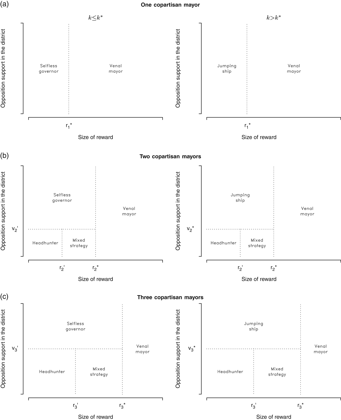
We now turn to a description of the model’s equilibria. We proceed by iterative elimination of suboptimal strategies, emphasizing the threshold values of reward (r), cost of campaigning (k), and opposition normal vote (v) for which (some) players have dominant strategies. We then find optimal responses for other players. When there are no equilibria in pure strategies, we show that equilibria exist in mixed strategies. Figure 1 guides our discussion of the equilibria that exist when there are one, two, and three copartisan mayors in a district.Footnote ¹¹ Notice that the scenarios with two and three copartisan mayors are similar, but in the one-copartisan-mayor scenario there are no equilibria in mixed strategies.

Figure 1.

Equilibria under three alternative scenarios. The horizontal and vertical axes indicate the values of reward size (r) and opposition’s support in the district (v) that serve as cutpoints among the different equilibria. Note that $$r_{3}^{{\asterisk}} \,\gt\,r_{2}^{{\asterisk}} \,\gt\,r_{1}^{{\asterisk}} $$.

The threshold $$r_{3}^{{\asterisk}} $$ establishes a sufficient condition for mayoral mobilization, as can be seen along the horizontal axis in Figure 1. As in other delegation games (e.g., Besley Reference Besley2007) a “disciplined” bad-type can masquerade as a good type, which is beneficial for the party in the short-term (it brings votes) but detrimental in the long run because the governor could end up rewarding a bad type that will weaken the party. We say such disciplined behavior is “venal” because the bad-type mayor only works on behalf of the party when he has a shot at getting a reward. Specifically, the size of the effort-inducing reward $$r_{3}^{{\asterisk}} $$ depends on (i) the relative mobilizing capacity of the governor (s), (ii) the abundance of good types in the population (τ), (iii) the cost of exerting effort (f), and (iv) the uncertainty surrounding the election outcome (ψ). If governors have a mobilizing advantage (high s) or if the expected incidence of good types is high (high τ), the bad type will reason that his contribution is unlikely to lead to victory (his relative mobilization capacity is low and other mayors are probably of good type, therefore already campaigning and likely to get the reward if they are monitored). Given the low chance of being rewarded, bad types will only bother to exert effort if the reward is very large, or the cost of exerting effort is very low.Footnote ¹² Similarly, as the translation of effort into outcomes becomes more reliable (i.e., as ψ increases), the size of the effort-inducing reward diminishes: the cost of effort is independent of the electoral outcome, so an increase in the reliability of effort will induce more of it. A venal mayor equilibrium also exists in scenarios with one or two copartisan candidates, though the effort-inducing reward in these circumstances is smaller (i.e., $$r_{1}^{{\asterisk}} \,\lt\,r_{2}^{{\asterisk}} \,\lt\,r_{3}^{{\asterisk}} $$; see Appendix A). This follows from the higher probability that a bad-type mayor will obtain the reward when there is less competition from other copartisan mayors, and we will make use of it in deriving a testable implication of the model.

When the reward is low ($$r\,\lt\,r_{3}^{{\asterisk}} $$), we find two equilibria in pure strategies in which bad mayors do not exert effort, and one equilibrium in mixed strategies in which bad mayors exert effort only some of the time. The first of the pure-strategy equilibria is a headhunter monitoring equilibrium:

The intuition is that mayors know there is a high probability that a copartisan will carry the district even if they do nothing (because the opposition normal vote, v, is low enough). Since the reward for exerting effort is low, bad types lack an incentive to help regardless of the governor’s actions. But the governor can still monitor mayors to find a good type to reward after the election. In fact, monitoring and low rewards go hand-in-hand: because the reward is low, bad types do not consider it worth their while to try to distinguish themselves by exerting effort. After all, if the governor monitors some other bad type and finds him wanting, there is still a chance they might get the reward without having exerted effort. The requirement that v be low enough is also intuitive. Doling out the reward requires winning the district first; if the election is lost, finding that a mayor is of good type is worthless. Thus, when the opposition enjoys an electoral advantage the governor has incentives to campaign rather than to monitor the mayors. But if the governor’s party can expect to win, the benefits of identifying a good mayor outweigh those of campaigning: in these circumstances, effort exerted by a monitored mayor is superfluous in winning the district, but it still reveals useful information about the mayor’s type. Appendix A shows that a similar logic applies in a scenario with two copartisan mayors, but not in the one-mayor scenario, as the governor has no incentive to monitor a mayor for whom, were he found to be a bad type, there is no potential substitute.

The second equilibrium in pure strategies in a low reward environment is one where a selfless governor “takes one for the team” while mayors coast. This equilibrium can only be sustained if the cost of campaigning is low enough; otherwise, both the probability of carrying the district and the potential mayoral reward are so low that local politicians—both mayors and governor—lack incentives to mobilize on behalf of copartisan candidates and choose to jump ship instead.

The main factor driving a governor to act selflessly is the low cost of campaigning. By choosing to campaign on behalf of her party, the governor has a shot at rewarding a mayor—an eventual ally. The cost k that the governor is willing to pay increases with the amount of electoral certainty (ψ), the efficiency of her own effort (s), and the incidence of good types in the population (τ), though this cost does not vary across scenarios (i.e., $$k_{1}^{{\asterisk}} {\equals}k_{2}^{{\asterisk}} {\equals}k_{3}^{{\asterisk}} $$; see Appendix A). The governor will only act selflessly if the party is at least minimally competitive (relatively low v), because this gives her a shot at promoting a mayor believed to be of good type. If the party is not minimally competitive, neither the governor nor the mayors have incentives to campaign at all, leading to a “jumping ship” equilibrium.

Finally, when the effort-inducing reward increases beyond $$r_{3}^{'} $$ but still remains below $$r_{3}^{{\asterisk}} $$, players adopt a mixed-strategy equilibrium:

Intuitively, if bad mayors coast, the governor prefers to monitor them in order to identify a good one for promotion; but since the reward is large enough to induce bad mayors to exert effort if they expect to be monitored, the governor will prefer not to monitor anybody, and so on. To put it differently, the governor only wants to monitor when bad mayors do not exert effort, while bad mayors only want to exert effort when the governor is monitoring them. Thus governor and mayors will choose a combination of actions to make each other indifferent between exerting effort or not, and monitoring or not. Appendix A shows how the mixing probabilities depend on the cost of monitoring (g), the cost of exerting effort (f), and the size of the reward (r). The Appendix also shows that a similar logic applies to a scenario with two mayors, but if there is a single copartisan mayor a mixed strategy equilibrium does not exist because the governor never has an incentive to monitor.

Observable implications of the model

Ideally, we would evaluate these propositions by carefully measuring the amount of effort that mayors exert in favor of copartisan candidates and by gauging the level of involvement of governors in a campaign or in monitoring mayoral behavior. Neither individual nor team effort are readily observable—neither by us nor by party leaders, which is an important part of our argument. However, we can inspect whether a congressional candidate carries the election at the district level, which is the outcome of interest in our theory.

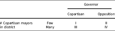
Thus, we focus on comparing a congressional candidate’s probability of winning across electoral districts that comprise several municipalities. As shown in Table 1, these districts vary along two dimensions: (i) the proportion of municipalities within the district that are governed by copartisan mayors; and (ii) the governor’s copartisan status. All other things equal, both factors should have a positive effect on the probability that a party captures a district: on the one hand, the governor may campaign or monitor mayors, thus inducing them to exert effort; on the other, the more mayors there are, the more likely it is that some of them are of good type, and thus will campaign regardless of the governor’s behavior. Yet this only holds as long as we consider the governor or the mayors in isolation; if players interact with each other, some may try to pass the responsibility for mobilizing voters to others, and thus increasing the number of copartisans in a district does not necessarily produce a corresponding increase in the party’s chances of carrying the district.

Table 1.

Four Possible Combinations of Copartisan Officials

In other words, we claim that having a copartisan governor will exert a dampening effect on the degree of mayoral mobilization in a district. The intuition behind this claim is the following. When there is no copartisan governor (quadrants II or IV in Table 1), only good mayors will exert effort. To the extent that the probability of having a good mayor is increasing on the number of mayors in a district, having many mayors will increase a party’s electoral performance in the district. When there is a copartisan governor, this logic continues to hold for good mayors, but now bad-quality mayors may also exert effort if conditions are right. Yet these conditions are very specific: bad-quality mayors never exert effort in three of the five equilibria derived above (selfless governor, headhunter, or jumping ship), and in another (mixed strategies) they exert effort only some of the time; only in the venal mayor equilibrium do bad-type mayors consistently exert effort on behalf of the party. And moving from the top to the bottom of Figure 1 shows that for a given reward size, the area for which the venal mayor equilibrium holds—that is, the range of combinations of reward size and opposition support—is decreasing on the number of mayors in a district. To put it differently, bad-quality mayors never have as many incentives to exert effort than when they are “alone” with the governor.

Such incentives are reinforced by the governor’s behavior. As Figure 1 shows, the governor never has incentives to campaign if k>k*, which does not depend on the number of mayors. Yet whether the governor campaigns or monitors does depend on the number of mayors in a district. Figure 1 indicates that when there is a single mayor, the governor always campaigns (as long as k>k*); as the number of mayors increases, however, the values of the parameters for which the governor campaigns decreases, because the governor prefers to monitor mayors in order to find a good one for promotion. Of course, this is good enough for the governor, and may be good for the party insofar as it fosters the promotion of good politicians in the long run; but in the current election, it means that the governor will campaign less, and thus the party’s probability of winning the district will be lower than could be the case.

In sum, having more copartisan officials in a district would be unquestionably good if such officials always exerted effort on behalf of their party, but the model shows that the simultaneous provision of effort by the governor and the mayors is both relatively rare and decreasing on the number of mayors in a district. This results from the combination of two mechanisms. On the one hand, mayors face a cooperation problem: the more numerous they are, the more likely it is that the party will win the district, but the less likely that any given mayor will be promoted; thus, unless the reward is very large, bad mayors prefer to coast rather than work for the party. On the other hand, the governor finds it less attractive to campaign but more rewarding to monitor mayors in order to identify a good one for promotion. That is, having more mayors increases the number of good types that always exert effort, but also discourages both the governor and bad-type mayors from campaigning, (partially) offsetting the benefits of having more good mayors.

Note that we do not claim that having a governor is “bad” for a party; on the contrary, we expect a congressional candidate to do better when there is a copartisan governor. Rather, our claim is that a copartisan governor should dampen the effect of having more copartisan mayors in a district. Formally, let the probability that party j captures district d depend on both the number of copartisan mayors in d, M _jd , and whether there is a copartisan governor (G _jd =1), such that

$$\Pr ({\rm Win}_{{jd}} {\equals}1\,\mid\,G_{{jd}} {\equals}1){\equals}\beta _{0} {\plus}\beta _{1} M_{{jd}} $$

$$\Pr ({\rm Win}_{{jd}} {\equals}1\,\mid\,G_{{jd}} {\equals}0){\equals}\gamma _{0} {\plus}\gamma _{1} M_{{jd}} $$

Our claim is that β ₀>γ ₀, which is an expectation for which little theoretical insight into political behavior is needed, but also that β ₁<γ ₁, which is not such an obvious claim. The latter difference corresponds to the dampening effect that follows from our formal argument.

Before considering the empirical evidence, we comment briefly on the plausibility of the assumptions behind our model. First, our argument applies more clearly to strong party organizations that are able to promote politicians within the party ranks. It would certainly be more difficult to see these dilemmas in parties that lack minimal control over nomination decisions. With this caveat in mind, the gist of our argument holds if we assume that the congressional candidate, rather than the governor, performs the task of monitoring. Even more so than with the governor, the congressional candidate would face a trade-off between campaigning and monitoring. We anticipate that the argument would hold as well if, more realistically, we allow for the possibility that the governor may monitor and/or reward several mayors. What matters in our model is the characterization of rewards (gubernatorial support) as limited, an assumption that is valid as long as the number of mayors that aspire to improve their careers is larger than the number of promotion opportunities within the party, which seems reasonable in most contexts.

Estimating the impact of copartisan mayors and governors

We examine our claims using data from congressional elections in Mexico between 2000 and 2012. Mexico provides an ideal scenario for examining these predictions. First, several Mexican states have electoral calendars that are not concurrent with national elections, which helps us distinguish the effect of mobilization in support of a copartisan candidate from the “reverse coattail” effect of mobilization to secure control of the mayor’s office; indeed, we restrict the analysis to states where local and federal elections take place in different years. Second, Mexican governors play an important role in promoting their copartisan’s future careers (Kerevel Reference Kerevel2015). Third, during the period under study the Mexican constitution barred all elected officials from seeking consecutive reelection at the end of their term. This ensures that any positive effect that governors and mayors exert on the probability of victory of their copartisans is a consequence of their effort on behalf of copartisan candidates, rather than an attempt to secure their own reelections. Similarly, the probability of winning the district cannot be attributed to an incumbent legislator’s advantage, because legislators are also limited to one term in office. Finally, most Mexican municipalities are nested within single-member districts, which in turn are nested within states. Specifically, the Mexican lower chamber is elected using a mixed-member system: 200 legislators are elected in five proportional-representation districts, the remaining 300 in single-member districts. We focus exclusively on the single-member constituencies, most of which comprise several municipalities.Footnote ¹³

Our study is based on a set of 461 district-elections throughout five federal elections scheduled triennially from 2000 to 2012. The number of municipalities per district ranges from 1 to 40, with a median of 9 and an average of 9.5. Each district-election yields two observations—one for the party that controls the governorship at the time of the election and one for the runner-up party in the previous gubernatorial election—which we separate into different sets to estimate two models—one for candidates with copartisan governors and the other for candidates without copartisan governors.Footnote ¹⁴ We follow this approach because even though Mexico has a three-party system at the national level, during the period under observation subnational competition was mostly bipartisan: in most states the Partido Revolucionario Institucional (PRI) competed against a single large opposition party, either the center-right Partido Acción Nacional (PAN) or the center-left Partido de la Revolución Democrática (PRD). For example, the PRI governed the state of Chihuahua between 1998 and 2016, having beaten PAN candidates in what were practically two-party races. Hence, districts in Chihuahua furnish two sets of observations: one set for PRI mayors and congressional candidates operating under a copartisan PRI governor, and one set for PAN mayors and congressional candidates that operate under an opposition (i.e., PRI) governor.

The outcome is an indicator of whether the congressional candidate carried district d and the parameter of interest is the effect of the proportion of copartisan mayors in the district (i.e., β ₁ and γ ₁). Many factors extraneous to our model have an effect on both mayoral behavior and a congressional candidate’s probability of victory; moreover, we cannot feasibly measure a host of factors within our model (size of reward, gubernatorial capacity) that would need to remain constant in order to verify the existence of a dampening effect. In short, we cannot claim that the assignment of proportion of copartisan mayors across districts is exogenous, which is an important limitation in our analysis.Footnote ¹⁵ We do control for observable confounders in our models: the party’s margin of victory in the municipality in the previous district-level race, the municipality’s poverty level, and a quadratic polynomial of the party’s normal vote share in the district.Footnote ¹⁶

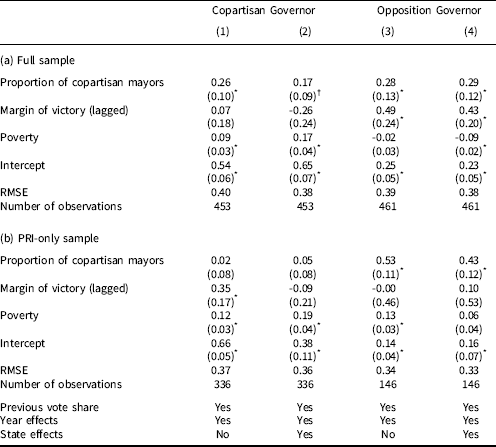
Table 2 displays linear probability estimates of how the proportion of copartisan mayors in a district affects the probability that the congressional candidate will win the district.Footnote ¹⁷ We report separate results for candidates with and without copartisan governors. Models 1 and 3 control for margin of victory, normal vote share, poverty, and year fixed effects; Models 2 and 4 add state fixed effects. In Panel (a), we consider results based on the full sample of districts and municipalities they contain, which include governors and mayors from the three main political parties. In line with expectations, comparing the intercept estimates in Models 1–2 against those in Models 3–4 confirms that, when the proportion of copartisan mayors in the district is nil, the probability that a congressional candidate will carry a district in a state with a copartisan governor is larger than the probability that she will win the election if the state is led by a non-copartisan governor. In addition, we find some evidence of a dampening effect, but this evidence is not entirely consistent with our claims. To see this, consider that the point estimate of the effect parameter of proportion of copartisan mayors is positive in districts with copartisan governors (Models 1–2), though the effect is only statistically significant at the 95% confidence level in Model 1, which excludes state-level fixed effects. In contrast, the positive estimates for the effect parameters of proportion of copartisan mayors in districts with non-copartisan governors (Models 3–4) are of larger magnitude and statistically significant at the 95% confidence level.

Table 2.

A Congressional Candidate’s Probability of Victory as a Function of Proportion of Copartisan Mayors

* p<0.05;^†p<0.10. OLS estimates. Standard errors clustered by state in parentheses.

The dampening effect we expect requires a difference-of-means test between the coefficients for proportion of copartisan mayors in Models 1 and 3 or Models 2 and 4, respectively. These tests indicate that the differences between the coefficients in Models 1–2 and 3–4 are not statistically significant, i.e., we cannot discard the possibility that the coefficients may in fact be equal. Nonetheless, a simple difference-of-coefficients test is inappropriate in this case because the samples are not independent, as the same district enters the first sample with a copartisan governor for one candidate and the second sample with an opposition governor for a second candidate. Thus, outcomes across samples are negatively correlated: a better performance for the governor’s party likely implies a worse performance for the runner-up’s, and vice versa.

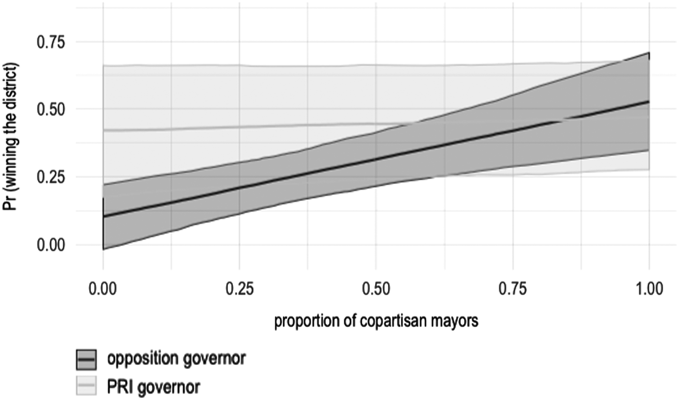
To break this dependence across samples, Panel (b) in Table 2 replicates the same four models, but limiting the analysis to PRI congressional candidates. As Mexico’s erstwhile hegemonic party, the PRI came in first or second place in almost all gubernatorial elections held between 2000 and 2012.Footnote ¹⁸ This ensures that the counterfactuals for districts in which the PRI was the runner-up in the previous gubernatorial election are districts in which the PRI controlled the governorship, and vice versa. Despite a considerable reduction in sample size, results in Table 2b are consistent with the expected dampening effect: when there is a PRI governor, the coefficient of proportion of copartisan mayors is essentially zero, while in opposition-governed states the estimated coefficient ranges between 0.43 (se=0.12) and 0.53 (se=0.11), and is statistically significant at conventional levels. Difference-of-means tests between the coefficients of Models 1–2 and 3–4 are also statistically significant. To illustrate this finding, Figure 2 shows the probability that the PRI will carry a district conditional on the existence of a copartisan or opposition governor and the proportion of the district’s population governed by copartisan mayors, while holding all other variables at their means: when there is a copartisan governor, the probability of winning is large, but it remains essentially flat as the proportion of copartisan mayors increase. But if the governor is not a priísta, increasing the proportion of copartisan mayors has a large effect on the probability that the PRI will win the district.

Figure 2.

Predicted probability (+95% CI) that the PRI will capture a district, conditional on proportion of copartisan mayors and copartisan governor, based on models reported in columns 2 and 4 of Table 2b.

Robustness checks

We check the robustness of the dampening effect in several ways. First, Table A8 in Appendix C shows that proportion of copartisan mayors has no effect on a congressional candidate’s vote share or margin of victory at the district level. This is not entirely surprising, as none of these races are strictly bipartisan. A party may carry a district even with a lower vote share, as long as the first loser in the previous election loses even more votes. Second, controlling for the number of municipalities in the district barely changes our estimates (see Table A10 in Appendix C). Third, it may be argued that the results reflect a “ceiling effect” rather than a dampening one. This is unlikely because most vote shares range between 0.35 and 0.55, leaving space for growth. Furthermore, a ceiling story predicts that any mayor would do his best to mobilize in favor of a copartisan candidate running for Congress, but the regression discontinuity estimates reported in Table A11 in Appendix C show a negative incumbency effect of mayors on copartisan congressional candidates. This seems puzzling at first sight, but keep in mind that this estimate represents an average treatment effect that pools all mayors together, regardless of how many copartisan mayors exist in their district. In contrast, our argument and analysis focus on groups of mayors, considering explicitly the proportion of municipalities controlled by copartisan mayors in any given district. Fourth, the dampening effect could result from the fact that the efforts of governors and mayors are partial substitutes: if the governor’s campaigning effort suffices to convince voters, the help of copartisan mayors will be superfluous. Against this interpretation, in Table A12 in Appendix C we report regression discontinuity estimates that show that PRI mayors exert a larger effect on turnout in the presence of a copartisan governor, but only if there are few copartisan mayors in the district.