INTRODUCTION
Nitrogen (N) is the main nutrient affecting crop growth and yield formation, but at the same time excessive N in relation to crop N requirements has substantial negative environmental effects (Sutton et al. Reference Sutton, Erisman, Leip, van Grinsven and Winiwarter2011). Effective N fertilizer management is therefore crucial for optimizing crop yields, maximizing farmer income and minimizing negative environmental impacts from reactive N flows. Climate change will directly and indirectly change crop N demand, N mineralization and leaching (Stuart et al. Reference Stuart, Gooddy, Bloomfield and Williams2011; Patil et al. Reference Patil, Lægdsmand, Olesen and Porter2012; Doltra et al. Reference Doltra, Laegsmand and Olesen2014). This will make management of the agricultural N cycle even more challenging in future than it is at present.
Crop models have been widely applied for optimizing N management in agriculture (Shaffer Reference Shaffer2002; Kersebaum et al. Reference Kersebaum, Lorenz, Reuter, Schwarz, Wegehenkel and Wendroth2005; Rahn et al. Reference Rahn, Zhang, Lillywhite, Ramos, Doltra, de Paz, Riley, Fink, Nendel, Thorup-Kristensen, Pedersen, Piro, Venezia, Firth, Schmutz, Rayns and Strohmeyer2010; Nendel et al. Reference Nendel, Venezia, Piro, Ren, Lillywhite and Rahn2013). They have been important means in estimating the effect of N fertilizer application rates and timing on both crop yield (Dobermann et al. Reference Dobermann, Dawe, Roetter and Cassman2000; Cassman et al. Reference Cassman, Dobermann, Walters and Yang2003; Nykänen et al. Reference Nykänen, Salo and Granstedt2009) and N leaching (Wolf et al. Reference Wolf, Hack-ten Broeke and Rötter2005; Cannavo et al. Reference Cannavo, Recous, Parnaudeau and Reau2008; Hyytiäinen et al. Reference Hyytiäinen, Niemi, Koikkalainen, Palosuo and Salo2011).
For Europe, four crop model inter-comparison studies were set up during 2007–2010 based on the need for evaluating performance of crop models against data from field experiments under current climate as a basis and first step for judging their utility for climate change impact assessments (Monteith Reference Monteith1981; Rötter et al. Reference Rötter, Carter, Olesen and Porter2011a ; Wheeler & von Braun Reference Wheeler and von Braun2013). These inter-comparisons were performed within the framework of COST action 734 seeking coverage of the most widely used and accessible crop simulation models: two of the comparisons were for winter wheat (Palosuo et al. Reference Palosuo, Kersebaum, Angulo, Hlavinka, Moriondo, Olesen, Patil, Ruget, Rumbaur, Takac, Trnka, Bindi, Caldag, Ewert, Ferrise, Mirschel, Saylan, Siska and Rötter2011) and spring barley (Rötter et al. Reference Rötter, Palosuo, Kersebaum, Angulo, Bindi, Ewert, Ferrise, Hlavinka, Moriondo, Nendel, Olesen, Patil, Ruget, Takac and Trnka2012) across multiple sites in Europe with limited calibration and one for heat and drought sensitivity of wheat and maize at two Austrian locations (Eitzinger et al. Reference Eitzinger, Thaler, Schmid, Strauss, Ferrise, Moriondo, Bindi, Palosuo, Rötter, Kersebaum, Olesen, Patil, Saylan, Çaldag and Çaylak2013). The fourth inter-comparison presented here was conducted using comprehensive barley data sets from one Finnish location and included a comparison of the capability of 11 different models to simulate yield response to varying N inputs.
The main objective of the current model inter-comparison study was to assess and compare the uncertainties and capability of different models in simulating spring barley yield responses to a range of N application rates from none to high (150 kg N/ha) when provided with a comprehensive data set for model calibration. Eleven crop models were run at the Jokioinen site in Finland for two growing seasons of spring barley for model calibration and one season for model testing.
MATERIAL AND METHODS
Models
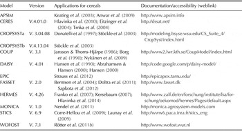
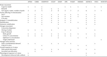
The 11 crop simulation models included in the inter-comparison were APSIM, CERES, CROPSYST, COUP, DAISY, EPIC, FASSET, HERMES, MONICA, STICS and WOFOST (Table 1). Models were first calibrated and then tested against different N fertilizer rates. Details about the models used can be obtained from the main references gathered by Rötter et al. (Reference Rötter, Palosuo, Kersebaum, Angulo, Bindi, Ewert, Ferrise, Hlavinka, Moriondo, Nendel, Olesen, Patil, Ruget, Takac and Trnka2012), except for APSIM (Probert et al. Reference Probert, Dimes, Keating, Dalal and Strong1998; Keating et al. Reference Keating, Carberry, Hammer, Probert, Robertson, Holzworth, Huth, Hargreaves, Meinke, Hochman, McLean, Verburg, Snow, Dimes, Silburn, Wang, Brown, Bristow, Asseng, Chapman, McCown, Freebairn and Smith2003), COUP (Jansson & Karlberg Reference Jansson and Karlberg2012) and EPIC (Williams Reference Williams and Singh1995). Table 2 provides a characterization of process descriptions on N dynamics for the various models. CROPSYST was operated by two separate teams using different model versions and calibration approaches. The results for these are presented as CROPSYST a and b.
Model version applied in the current study, references to papers with model descriptions and model web address

Modelling approaches applied in the current study regarding the major processes determining nitrogen (N) response on crop growth and nitrogen dynamics in soil
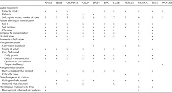
x denotes that approach was used in the model.
All models were dynamic and worked on a daily time step. Most of them used similar process descriptions of the N cycle. Below, some differences among models in simulating major processes are described. For more details of N processes, the reader is referred to Table 2 and for other biophysical processes, to Palosuo et al. (Reference Palosuo, Kersebaum, Angulo, Hlavinka, Moriondo, Olesen, Patil, Ruget, Rumbaur, Takac, Trnka, Bindi, Caldag, Ewert, Ferrise, Mirschel, Saylan, Siska and Rötter2011) and Rötter et al. (Reference Rötter, Palosuo, Kersebaum, Angulo, Bindi, Ewert, Ferrise, Hlavinka, Moriondo, Nendel, Olesen, Patil, Ruget, Takac and Trnka2012):
-
• N demand. Most of the models determined crop N demand according to the daily growth and the critical N concentration needed for accumulated biomass (Table 2). Some models applied an optimum N concentration curve (DAISY, HERMES, STICS) or factor (MONICA).
-
• N uptake. Most models took up soil N according to crop N demand, soil available N, soil moisture, root length distribution and N transport rates in soil (Table 2). CROPSYST did not provide grain N content. It evaluated N uptake in total aboveground biomass, but did not estimate the proportion of N in grains. WOFOST used the QUantitative Evaluation of the Fertility of Tropical Soils (QUEFTS) approach to estimate N supply from soil and N uptake by the crop during the growing season (Janssen et al. Reference Janssen, Guiking, van der Eijk, Smaling, Wolf and van Reuler1990).
-
• N stress. Most of the models estimated N stress from the difference or ratio between daily or cumulative N demand and crop N uptake (Table 2). Lack of N determined by N concentrations dropping below the critical concentration – lead in most models to depressed daily dry matter (DM) growth, reduced leaf area expansion (FASSET, STICS), decreased gross photosynthesis (DAISY), and to enhanced root biomass allocation in some of the models (e.g. COUP, FASSET). STICS also reduced grain number due to N stress at certain developmental stages.
-
• N mineralization from soil organic matter. Most of the models divided the soil organic matter pool into 2–7 interconnected (conceptual) sub-pools of different mineralization rates (Table 2). Some models calculated N mineralization from C turn-over (DAISY, FASSET, MONICA), while others calculated N mineralization directly, without any link to C dynamics (HERMES, STICS). Mineralization of soil organic matter was controlled at least by soil temperature and moisture. In addition, in some models soil clay content (MONICA, STICS, DAISY), soil oxygen concentration (MONICA) and soil calcium contents (STICS) were used as control variables for N mineralization.
-
• Vertical movement of water in soil. Eight out of 11 models used a simple capacity or tipping bucket approach for soil water balance (Table 2). COUP and DAISY applied the more detailed Richard's approach for soil water movement (Richards Reference Richards1931). CROPSYST users could select either of the approaches for soil water movement, and capacity approach was used by CROPSYSTa and Richard's approach by CROPSYSTb.
-
• Vertical movement of N in soil. N movement was based mostly on the convection–dispersion equation or complete mixing of the flowing solute with the resident solute (Table 2). FASSET used a solute leaching intermediate model (Addiscott & Whitmore Reference Addiscott and Whitmore1991), and STICS used a reservoir with variable mixing depths (Burns Reference Burns1974). WOFOST did not calculate N movement or leaching. HERMES and MONICA considered upward movement by capillary rise if a shallow groundwater table was present.
-
• Denitrification. N loss due to denitrification was modelled as a function of soil temperature and water content in all models except WOFOST that did not simulate processes of soil N dynamics. Ammonia volatilization was included in CROPSYST, DAISY, MONICA and STICS only.
Study site
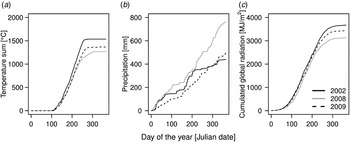
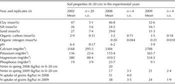
The model inter-comparison study was carried out using data from field experiments conducted in the years 2002, 2008 and 2009 at Jokioinen, southern Finland (60°42′N, 23°30′E 104 m a.s.l). In Jokioinen during 1980–2010, temperature sum (>5 °C base temperature) in May–September averaged 1244 °Cd and the precipitation sum 317 mm, which created typical conditions for spring barley production in a boreal climate. The experiments in 2002 and 2008 were conducted on the same field, while the experimental field in 2009 was located 5 km northeast of the former site. Both sites were c. 200 m from the river Loimijoki and their soil properties (Table 3) and crop rotation were considered similar enough to allow simulations with the same soil chemical and physical characteristics (Table 4). The soil type was sandy clay in the top layer (0–30 cm) and heavy clay below 30 cm. The soil was classified as Vertic Cambisol (Yli-Halla & Mokma Reference Yli-Halla and Mokma2001). Temperature (>5 °C), global radiation and precipitation sums from May to September in each growing season are presented in Fig. 1. In the growing season 2002, mean temperature (14·6 °C) was higher than the long-term average (13·1 °C, averaged over 1980–2010), while in 2008 and 2009 mean temperatures were 12·6 and 13·6 °C, respectively. Precipitation during the modelled growing seasons in May–September were lower than long-term average (317 mm, averaged over 1980–2010) amounting to 219, 288 and 246 mm, respectively, in 2002, 2008 and 2009. In 2008, there was a rain event of 47 mm on 7–8 August. For the cultivation of spring cereals in boreal climates it is known that climatic and soil conditions 2 months after sowing are crucial for crop yield establishment and small differences during early growth may have large implications for final yield (Håkansson et al. Reference Håkansson, Myrbeck and Etana2002; Pietola & Tanni Reference Pietola and Tanni2003). After snow melting, water flows to the sub-soil drainage system and soil dries to field capacity, and soil layers below 5 cm only start to dry after soil preparation and sowing. Groundwater level decreases from the depth of 30–40 cm after soil frost melting to below 2 m depth in the middle of the growing season.
(a) Temperature sum (>5 °C) (°C), (b) cumulated precipitation (mm) and (c) cumulated global radiation (MJ/m2) at Jokioinen in 2002, 2008 and 2009.

Detailed soil properties, soil inorganic nitrogen (N) in spring (Nmin) and grain N uptake of the unfertilized treatments in 2008 and 2009

Soil characteristics of the study site used in the modelling exercise

HC, hydraulic conductivity; N, nitrogen.
* mm water at field capacity (fc) and wilting point (wp) in specific root zone.
† Hydraulic conductivity including macropores.
The data from 2002 originated from a spatial soil mapping experiment (Farkas et al. Reference Farkas, Ristolainen and Alakukku2006), where soil physical conditions were measured and compared with crop growth from the 20 replicates. In 2008 and 2009, data were collected from a fertilizer experiment, with mineral N fertilizer rates from 0 to 150 kg N/ha at 30 kg N/ha intervals (designated as N0, N30 and so on up to N150). The experimental design was randomized complete blocks with four replicates in both years. Plot size was 25 × 3 m2 and yields were harvested from 50 m2 in 2008 and 35 m2 in 2009. Preceding crops were barley for 2008 and 2009, and spring wheat for 2002. Initial soil inorganic N content was measured from 0–30 cm soil layer and was 20–24 kg N/ha at the time of sowing. Previous measurements from a similar clay soil (Pietola et al. Reference Pietola, Tanni and Elonen1999; Pietola & Tanni Reference Pietola and Tanni2003) and sampling in spring 2009 provided information that the soil inorganic N in layer 30–90 cm was only 8–10 kg N/ha: this information was also provided for the modellers. Soil water content was slightly below field capacity (<40% vol.) at the time of sowing.
In the experimental years, compound nitrogen : phosphorus : potassium (NPK) fertilizer (17% N as ammonium nitrate) was placed between every second seed row at the time of sowing. Distance between seed rows was 12·5 cm. Spring barley cultivar Annabell (two-row) was used in all experimental years and the target seeding density was 500 plants/m2. In all experiments, the plots were kept weed-free and no interference from pests or diseases was observed. Management practices followed the best practices in the region and regulations of the Finnish Agri-environmental programme (Finnish Ministry of Agriculture and Forestry 2007).
Field observations
Each year, the leaf area index (LAI) was measured with a Sun Scan Canopy Analyser (Delta-T Devices, SS1, Cambridge, UK). In 2002 and 2008, LAI was measured four times in all treatments and in 2009 nine times in the N90 treatments and three times in all remaining treatments. Total above-ground biomass was sampled from all N treatments 41 days after sowing (DAS) in 2008 and 53 DAS in 2009. In 2009, nine sequential biomass measurements were taken from the N90 treatment. Biomass samples were collected from a 0·25 m2 square in each plot and stubble was cut to a height of 2 cm above ground level. Grain yields were measured from 35 to 50 m2 areas within each plot with a combine harvester and all grain yields were calculated as dry weight. To measure harvest index, total above-ground biomass samples were taken in 2009 at harvest from N90 treatments. Individual grain weight and grain N concentration were measured from all N treatments in 2008 and 2009. Grain N uptake was calculated from grain N concentration and grain yield. Soil water content was measured in 2002 and in 2009 with gypsum blocks and tensiometers from 25 to 40 cm in 2002 and from 10, 20 to 30 cm in 2009. In 2008, soil water content measurements with time-domain reflectrometry probes were available from a nearby field experiment on similar clay soil (46% clay and 25 g organic C/kg soil in 0–20 cm) from the depths of 0–30 cm and 0–60 cm. This experiment was conducted for comparing different soil management methods, and the soil water content measurements were used from conventional mouldboard ploughing as that was the soil management of the field used for model calibration in 2008. Barley was estimated to be suffering from water stress when plant available water capacity (field capacity – wilting point) was decreased to 30%, which would correspond to 27 and 33% of volumetric water contents in 0–30 and 0–90 cm, respectively.
Setup of model inter-comparison
Information available for modellers for calibration
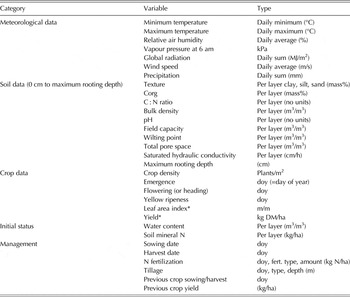
First, modellers were asked to calibrate their models for the experimental years 2002 and 2008. The data provided for this step (Table 5) included daily weather, crop management data (e.g. information on previous crop, tillage, sowing date and density, fertilization and harvest) and information on some basic soil properties (Table 4). Modellers were also provided with information on key phenological dates for spring barley during the growing periods. These included dates of sowing, emergence, flowering, yellow ripeness and harvest (Table 5). In addition, development of the LAI and the measured grain yield for the years 2002 and 2008 were provided for calibration. Calibration results of models for phenological dates, LAI and biomass development, grain yield and yield N uptake were gathered from the individual modellers for further analysis.
Input data provided to the models

DM, dry matter.
* Data not provided for the test year 2009.
Model testing
For the test year 2009, similar input data as for calibration years were delivered to the modellers, except for LAI and yield data. It was agreed that the crop phenology and soil parameters derived from the calibration were used in the testing exercise. After simulating crop growth for the test year, modellers provided their results on phenology, LAI and biomass development, yield and N uptake for analysis. After the first check of results, modellers were allowed to correct their results only if errors in inputs or other mistakes in the simulation setup were identified.
Methods for evaluating model performance and assessing uncertainties
For assessing and comparing model performance a set of statistical indicators was calculated in line with those reported by Palosuo et al. (Reference Palosuo, Kersebaum, Angulo, Hlavinka, Moriondo, Olesen, Patil, Ruget, Rumbaur, Takac, Trnka, Bindi, Caldag, Ewert, Ferrise, Mirschel, Saylan, Siska and Rötter2011) and Rötter et al. (Reference Rötter, Palosuo, Kersebaum, Angulo, Bindi, Ewert, Ferrise, Hlavinka, Moriondo, Nendel, Olesen, Patil, Ruget, Takac and Trnka2012). Grain DM yields and grain N content simulated by the various models and multi-model mean (MMM) were compared with observed values. Using multi-model ensembles has proved to provide robust estimates of growth and yield indicators (Palosuo et al. Reference Palosuo, Kersebaum, Angulo, Hlavinka, Moriondo, Olesen, Patil, Ruget, Rumbaur, Takac, Trnka, Bindi, Caldag, Ewert, Ferrise, Mirschel, Saylan, Siska and Rötter2011; Rötter et al. Reference Rötter, Palosuo, Kersebaum, Angulo, Bindi, Ewert, Ferrise, Hlavinka, Moriondo, Nendel, Olesen, Patil, Ruget, Takac and Trnka2012; Asseng et al. Reference Asseng, Ewert, Rosenzweig, Jones, Hatfield, Ruane, Boote, Thorburn, Rötter, Cammarano, Brisson, Basso, Martre, Aggarwal, Angulo, Bertuzzi, Biernath, Challinor, Doltra, Gayler, Goldberg, Grant, Heng, Hooker, Hunt, Ingwersen, Izaurralde, Kersebaum, Mueller, Naresh Kumar, Nendel, O'Leary, Olesen, Osborne, Palosuo, Priesack, Ripoche, Semenov, Shcherbak, Steduto, Stöckle, Stratonovitch, Streck, Supit, Tao, Travasso, Waha, Wallach, White, Williams and Wolf2013) and especially can provide better estimates than any individual model when multiple output variables are considered (Martre et al. Reference Martre, Wallach, Asseng, Ewert, Jones, Rötter, Boote, Ruane, Thorburn, Cammarano, Hatfield, Rosenzweig, Aggarwal, Angulo, Basso, Bertuzzi, Biernath, Challinor, Doltra, Gayler, Goldberg, Grant, Heng, Hooker, Hunt, Ingwersen, Izaurralde, Kersebaum, Müller, Naresh Kumar, Nendel, O'Leary, Olesen, Osborne, Palosuo, Priesack, Ripoche, Semenov, Shcherbak, Steduto, Stöckle, Stratonovitch, Streck, Supit, Tao, Travasso, Waha, White and Wolf2015).
The root mean square error (RMSE) was taken as a measure of relative average difference between the model estimates and measurements: it describes the average absolute deviations between the simulated and observed values.
 $${\rm RMSE}\, = \,\sqrt {\displaystyle{1 \over N}\sum\limits_{i = 1}^N {\left( {P_i - O_i} \right)^2}} $$
where N is the number of estimate–observation pairs, P i is the model prediction and O i is the observed value of the model i.
Mean bias error (MBE) was taken as an indicator of under- or over-estimation, i.e. the direction and magnitude of bias:
 $${\rm MBE} = N^{ - 1} \sum\limits_{i = 1}^N {\left( {P_i - O_i} \right)} $$
The index of agreement (IA) developed by Willmott (Reference Willmott1981) was used as a more general indicator of model efficiency.
 $${\rm IA} = 1 - \displaystyle{{N \times {\rm MSE}} \over {{\rm PE}}}$$
where
 ${\rm PE} = \sum\nolimits_{i = 1}^N {\left( {\left\vert {\dot P} \right\vert + \left\vert {\dot O} \right\vert} \right)^2} $
and where
 $\dot P = P_i - \overline O $
and
 $\dot O = O_i - \overline O $
, and
 $\overline O $
is the mean of the observed variable. Vertical bars indicate absolute values and MSE equals Eqn (1) without square root. The IA is the ratio of the sum of squared errors (N × MSE) and the largest potential error (PE) with respect to the mean of observed values. This parameter is sensitive to the model mean and to the peak values, and insensitive to low magnitude values (Willmott Reference Willmott1981). The IA can have values within the range [0, 1] and values closer to 1 indicate better simulation quality.
For the N fertilizer experiments, measurements from replicate plots (n = 4) were taken, allowing for an analysis of the uncertainties in observed LAI, yield and grain N uptake due to measurement errors and spatial variability in field conditions. Ranges and RMSE of simulated values were compared with standard deviations of observations.
Simulated yield responses to N were also analysed using the quadratic model that is commonly used to describe the relationship between fertilizer rates and yield responses (Schabenberger & Pierce Reference Schabenberger and Pierce2002):
 $$y\, = \,y_0 + aN + bN^{\rm 2} $$
where y is the grain yield, y 0 is the grain yield at N = 0, a and b are fitted constants, and N is the N fertilizer rate. The quadratic model was fitted to simulated grain yield of all crop models, MMM and observed data using the NLIN procedure of SAS software (SAS Institute Inc., Cary, NC, USA). The economically optimal N rate was calculated with 1€/kg N fertilizer cost and 0·15 €/kg DM price of barley grains, based roughly on N fertilizer and grain prices in Finland in 2000s, and then income was maximized by deducting fertilizer cost from the value of the barley yield. Maximizing Eqn (5) resulted in Eqn (6), which could be solved using only the fitted constants from Eqn (4).
 $$f\,(N) = 0.15 \times (y0 + aN + bN^{\rm 2} )-N\, \times \,{\rm 1}$$
 $$N\, = \displaystyle{{{\rm 1} - {\rm 0}{\rm {\cdot}15}a} \over {{\rm 0}{\rm {\cdot}15} \times {\rm 2}b}}$$
where f(N) is the gross profit (€/ha) the farmer earns due to N fertilizer.
RESULTS
Experimental years
The general weather conditions of the three seasons included in the current study were similar during the growing period for barley (Fig. 1). According to measured data from the sites and from the nearby field experiments (data not shown), soil moisture remained sufficient over all seasons in the 0–60 cm soil layer. However, measurements indicated dry soil (soil water content <30% of plant available water capacity) from 29 to 38 DAS in the uppermost (0–30 cm) soil layer in year 2002. In 2008 and 2009, the top layer dried <30% of plant available water capacity at 42 and 50 DAS, respectively. In the deeper (30–60 cm) soil layer, soil water contents decreased <30% of plant available water capacity around 75 DAS in 2002 and 2009 but at 55 DAS in 2008.
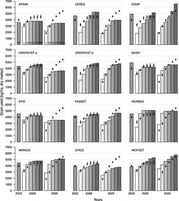
The observed maximum LAI of all N treatments (Fig. 6) and the LAI dynamics in N90 (data not shown) were similar in 2008 and 2009. Measured DM yields in 2002, 2008 and 2009 for the standard Finnish N rate (78 kg N/ha in 2002 and 90 kg N/ha in 2008 and 2009) were 4010 kg/ha (s.d. = 161 kg/ha, N = 20), 4430 kg/ha (s.d. = 305 kg/ha, N = 4) and 4560 kg/ha (s.d. = 109 kg/ha, N = 4), respectively. Twenty observation sites on the same field in 2002 showed a considerable variation (range 3390–4100 kg/ha). In 2008, measured grain yield without N fertilizer was considerably higher, 3200 kg/ha (s.d. = 268 kg/ha, N = 4) compared with non-fertilized yield of 2009 (1840 kg/ha, s.d. = 152 kg/ha, N = 4) or average yields in the non-fertilized controls of the Finnish field experiments at 2400 kg/ha (s.d. = 800 kg/ha, N = 60) (Valkama et al. Reference Valkama, Salo, Esala and Turtola2013). Yield response to N fertilizer was very different between 2008 and 2009, as in 2008 the N rate of 60 kg/ha led to 0·96 of maximum grain yield obtained with 150 kg N/ha, while in 2009 yield response to N fertilizer continued until 150 kg N/ha (Fig. 2).
Simulated (bars) and observed (dots) dry matter grain yield in 2002, 2008 and 2009. The bars on the observed yields show standard deviation.

Observed individual grain weight was clearly lower in 2008 (36 mg) than in 2002 (42 mg) and 2009 (47 mg) for treatments with standard N rates (78–90 kg/ha), which may have been the result of a shorter grain-filling period in 2002 and 2008 as compared with 2009. This was also found in data from farms of southern Finland where individual grain weight of cultivar Annabell was 37 mg in 2008 and 44 mg in 2009 (grain quality data of Finnish Food Safety Authority, unpublished). Field observations did not indicate any reasons (e.g. lodging or diseases) that would explain the difference in grain weights. The main observed difference between the growing seasons was the early and vigorous tillering after emergence in 2009 and a heavy rainfall event on 7–8 August 2008. In 2009, the low daily average temperature (7 °C lower than in 2008) 20–25 DAS, together with a 25 mm rainfall event (3–4 June) resulted in early and vigorous tillering. Field observations on 2 July 2009 counted 3–4 tillers in treatments with sufficient N rates (>60 kg/ha). In 2008 a heavy rainfall event caused soil water content to rise from 28 to 40% vol. in the 0–30 cm soil layer after 85 DAS, while in 2009, soil water content in 0–30 cm layer remained below 30% vol. until harvest.
Grain yield
Calibration
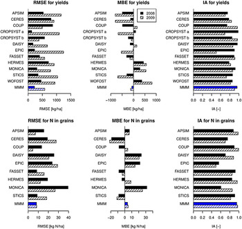
Grain yields were calibrated reasonably well in 2002 and 2008 (Figs 2 and 3). In 2002, simulated grain yields ranged between 3570 and 4920 kg DM/ha, i.e. –11 to +23% compared with an observed yield of 4000 kg/ha. In 2008, CROPSYSTa, DAISY, EPIC, FASSET, MONICA, STICS and WOFOST showed good performance with RMSE values lower than 500 kg/ha and IA values > 0·8 in calibration (Fig. 3). CERES, COUP and HERMES produced the highest RMSE values of 720–870 kg/ha in calibration and their IA values were still >0·7. APSIM, COUP and STICS under-estimated the grain yields, whereas HERMES, MONICA and WOFOST over-estimated yields (Fig. 3). In the 2008 experiment, standard deviation of observed grain yields in N treatments varied from 180 to 360 kg/ha, which means that the best model calibrations (CROPSYSTa, DAISY, EPIC, MONICA and STICS) were within the experimental error observed in the field. Multi-model mean produced RMSE values of 220 kg/ha and IA of 0·9 in 2008.
Statistical indicators of model performance for 2008 ( ) and 2009 (
 ). MMM shows the multi-model mean.

Testing against independent data set
For the test year 2009, the performance of models decreased compared with the calibration year 2008, as indicated by RMSE that approached 1000 kg/ha for several models (Fig. 3). In the group of well-calibrated models, CROPSYSTa, EPIC, STICS and WOFOST produced considerably higher RMSE for the test year. CROPSYSTb, DAISY and FASSET were able to retain their good performance with RMSE values <700 kg/ha and IA values still close to 0·9 for the test year.
In the yield observations within N treatments, standard deviation was low and varied from 70 to 180 kg/ha in 2009. Multi-model mean produced RMSE values of 540 kg/ha and IA value of 0·9 in 2009 (Fig. 3) showing that overall, model performances were not considerably weaker than in the calibration year 2008.
Yield response to Nitrogen
None of the models was able to reproduce the general pattern of observed grain yield fertilizer response of 2008 and 2009 simultaneously, which included a levelling off at medium N rate as in 2008 and a steep response beyond high N rate as in 2009. Observed grain DM yield response to N fertilizer in 2008 levelled off between N60 and N90 although the maximum yield of 4490 kg/ha (s.d. = 293 kg/ha) was recorded in the N150 treatment (Fig. 2). In the test year 2009, the observed grain yield response for N was considerably stronger and continued until N150 reaching 5420 kg/ha (s.d. = 107 kg/ha) of grain yield.
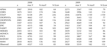
The fitted second degree polynomials showed that CERES, COUP and CROPSYSTb were calibrated to under-estimate grain yield without N fertilizer by >1000 kg/ha than was observed in 2008 (Table 6). The overall calibrated yield response to N in 2008 was best simulated by CROPSYSTa, DAISY, EPIC, MONICA, STICS, FASSET and WOFOST (Figs 2 and 3).
Second degree polynomials fitted for the model simulated, multi model mean (MMM) and observed grain dry matter yields in 2008 and 2009

a is yield without N fertilizer (kg DM/ha); max Y is the highest grain yield (kg DM/ha) obtained with the N rate; N maxY (kg N/ha); N Econ is the N rate (kg N/ha) to get the best economical result when the price ratio of 1 kg fertilizer to 1 kg grain is 6·67 (1/0·15), obtained by maximizing the differential of yield value (yield from second degree polynomial × grain price) and fertilizer cost.
The impacts of weather and management data provided on simulated yields were similar in 2008 and 2009 according to most models and they produced similar moderate N response curves for both years (Fig. 2 and Table 6). Based on these similar N response curves, DAISY, EPIC, HERMES, MONICA and WOFOST over-estimated the grain yield without N fertilizer by c. 1000 kg/ha or more (Fig. 3, Table 6). Despite using the same soil parameterization data and having similar weather conditions, APSIM, CERES, CROPSYSTa, DAISY, EPIC, MONICA and STICS estimated lower yield without N fertilizer in 2009 compared with 2008, as was also observed in the field experiment. However, the largest yield decrease among the models was only 700 kg/ha, while the actual yield decrease in the field was 1350 kg/ha.
Yield estimates of HERMES, MONICA and WOFOST were closest to the observed maximum yield of 5420 kg/ha (s.d. = 107 kg/ha), whereas COUP over-estimated maximum yield by 1130 kg/ha. COUP provided exceptional results as it was the only model that performed better in the test year than in calibration year 2008, and it showed a steep yield response to N in both years.
The majority of models simulated grain yield response to N fertilizer to level off at the same 90 kg N/ha N rate as in 2008 (Fig. 2, Table 6). However, COUP, STICS, FASSET and WOFOST estimated a higher yield response to N, levelling off only towards 120–150 kg N/ha in both 2008 and 2009. Economically optimum N rates were mostly lower than N rates giving the highest grain yields (biological optimum, Table 6). In 2009, yield response to N was both biologically and economically profitable until N150. FASSET and WOFOST succeeded in increasing their economically optimal N rates to N150 in 2009. The economical optimum of MMM was also increased from N90 in 2008 to N120 in 2009.
Nitrogen uptake
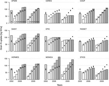
Information on N uptake in grain was not made available to the modellers in the calibration step. In the calibration year 2008, observed grain N uptake from the plots without N fertilizer averaged 51 kg N/ha (s.d. = 4 kg N/ha). The highest grain N uptake was 93 kg N/ha (s.d. = 6 kg N/ha) in the N150 treatment. In 2009, grain N uptake from the plots without N fertilizer averaged 25 kg N/ha (s.d. = 2 kg N/ha). The highest observed grain N uptake was 106 kg N/ha (s.d. = 1 kg N/ha) in N150 treatment.
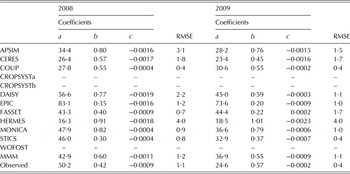
Models followed the pattern of increased N uptake in grain due to increased N fertilizer rates in both years (Fig. 4). The RMSE values of the models ranged from 10 to 40 kg N/ha in 2008 (Fig. 3) and from 5 to 30 kg N/ha in 2009, while RMSE of the MMM was 8 kg N/ha in both years. DAISY, EPIC and MONICA had a tendency to over-estimate the grain N uptake and CERES had a tendency to underestimate the grain N uptake. The IA values were close to 0·8 for all models except EPIC.
Measured nitrogen (N) in grain (dots) and model estimates (bars) in 2002, 2008 and 2009. CROPSYSTa, CROPSYSTb and WOFOST did not simulate grain N values. The bars on the observed N in grain show standard deviation.

All models, except EPIC, produced almost linear grain N uptake responses to N rate (Fig. 4), which were well described by the second-degree polynomials (Table 7). EPIC showed high and HERMES low grain N uptake of unfertilized barley in both years (Fig. 4 and Table 7). COUP and CERES simulated c. 25 kg N/ha uptake from unfertilized treatments, which under-estimated grain N uptake in 2008 but fitted well in 2009. STICS estimated best the crop N uptake in unfertilized barley, but STICS under-estimated N uptake in grain at the high N rates in 2009. MONICA and DAISY tended to over-estimate N in grains at high N rates.
Second degree polynomials to describe nitrogen (N) uptake (kg N/ha) in grains as function of fertilizer N rate (kg N/ha) (N in grains = a + b × N rate + c × (N rate)2)* for the model simulations, multi model mean (MMM) and observations in 2008 and 2009

Root mean square error (RMSE) shows the error between second degree polynomial equation and the modelled results.
* a, intercept; b, coefficient of the first degree term; c, coefficient of the second degree term.
Above-ground N uptake at maturity was reported by all models, except EPIC and WOFOST. On average, models allocated 0·68 of total above-ground N uptake to grains. The lowest proportion of N in grains from total above-ground N uptake, 0·56, was simulated by STICS and the highest, 0·79, by HERMES.
Soil water content
Similar to observations in 2002, CERES, DAISY, HERMES, MONICA, STICS and WOFOST estimated low soil water contents at 29–38 DAS (data not shown). In 2008, MONICA and STICS estimated a short period of water stress at 30 DAS in the 0–30 cm soil layer, which was not indicated by the measurements. Half of the models (CERES, CROPSYSTa, DAISY, EPIC, HERMES and MONICA) estimated, in line with observations that the uppermost (0–30 cm) soil water content decreased below 28% vol. (30% of plant available water left in soil) at 40 and 50 DAS in 2008 and 2009, respectively. For the 31–90 cm soil layer, all models estimated the soil water content higher than 33% vol. (30% of plant available water left in soil).
Crop phenology
Calibration results (2002 and 2008) for phenology (Fig. 5) did not match perfectly with the phenological data provided for calibration. The RMSE calculated on anthesis and maturity dates in 2002 and 2008 was 6–8 days for APSIM, CERES, CROPSYSTb, DAISY, FASSET, STICS and WOFOST but for COUP, CROPSYSTa, EPIC, HERMES and MONICA it was 10 days or more. Taking into account the uncertainties often related to observations of anthesis and, more generally, under partially N-stressed conditions, the results obtained by the models can be considered fairly satisfactory at this point. Model estimates for the length of growing period from sowing (growth stage (GS) 00 according to the BBCH scale; BBCH (Biologische Bundesanstallt Für Land-Und Forstwirtschaft) 1997) to physiological maturity (GS 90) were on average 93 and 100 days for 2002 and 2008, respectively, compared with the observed lengths of the growing period, 97 and 100 days. In particular, COUP, CROPSYSTa and EPIC showed fast phenological development (Fig. 5). Simulated emergence (GS 12) differed among the models only in APSIM, which estimated a 15-day longer period for emergence than the other models.
Comparison between observed and simulated periods from sowing to physiological maturity as bar lines. Observed (dotted lines) and simulated (dots) dates of emergence (growth stage (GS) 12), start of anthesis (GS 60) (completed anthesis –6 days) and physiological maturity (GS 90) in day of the year.

In the test year 2009, model estimates for the length of the growing season were on average 103 days, which is close to the observed length of the growing period, 102 days (Fig. 5). COUP, CROPSYSTa and EPIC were 5–10 days faster and DAISY, FASSET and STICS were 7 days slower in their development than observed for 2009.
The phenological development of MONICA and STICS reacted to low N supply by speeding up the development. In STICS this difference between unfertilized and N fertilized treatments was only one day, whereas MONICA estimated 11 days shorter growing period in 2008 and 9 days shorter in 2009 for the low-N treatments. In MONICA, anthesis began at the same time for all N treatments and physiological maturity was achieved faster with low N supply. While observed data showed no clear phenological response to N treatments, but differences of a few days may have gone unnoticed in the field observations.
Leaf area index, biomass and harvest index
Leaf area index
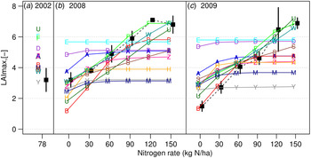
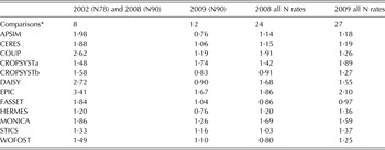
There were considerable differences between modelled and observed LAI (Fig. 6 and Table 8), even though the modellers were provided with observed LAI in 2002 and 2008 from all N treatments for calibration. In 2002, the observed maximum LAI was 3·7 (s.d. = 0·75) and in 2008 it increased with the increase in N rates from 3·2 (s.d. = 0·48) to 7·1 (s.d. = 0·07) (Fig. 6). The LAI responses to N fertilization during both calibration seasons were best estimated by HERMES (RMSE = 1·2) and STICS (RMSE = 1·3). COUP, DAISY, EPIC, FASSET and WOFOST tended to over-estimate the maximum LAI whereas CROPSYSTa and MONICA mostly under-estimated it (Fig. 6). The maximum LAI response to N in 2008 was modelled well by CROPSYSTb, FASSET and WOFOST with RMSE values <1·0 (Table 8).
Maximum leaf area index (LAI) of models and measurements in (a) 2002, (b) 2008 and (c) 2009. Models included are APSIM (A), CERES (B), COUP (U), CROPSYSTa (Y), CROPSYSTb (Z), DAISY (D), EPIC (E), FASSET (F), HERMES (H), MONICA (M), STICS (S) and WOFOST (W). Observations are marked with black squares and their standard deviation with black segment lines.

Model performance (root mean square error (RMSE) values) of estimated leaf area indices (LAIs) calculated based on data from two typical treatments of nitrogen (N) fertilization (78 or 90 kg N/ha) and for all treatments

* Number of comparisons between observations and modelling results.
In the test year 2009, observed maximum LAI increased from 1·5 (s.d. = 0·33) in the unfertilized treatment to 6·9 (s.d. = 0·35) in N150 treatment. Most models could not reproduce that but estimated similar maximum LAIs, between 4 and 5, as was observed in 2008 (Fig. 6). The models (COUP, FASSET and WOFOST) that simulated high maximum LAI, as was observed in 2008, fitted best to high LAI observations of 2009 (Fig. 6). The best estimates of the LAI curve of N90 in 2009 were simulated by APSIM, CROPSYSTb, DAISY and HERMES, all having RMSE < 1·0 (Table 8). FASSET estimated the steep LAI response to N rates best in the test year and its RMSE was 1·0 (Table 8).
Most models simulated similar maximum LAI responses to N for 2008 and 2009 and the majority were able to simulate an increase in maximum LAI with increasing N rates (Fig. 6).
The exceptions were EPIC, which estimated high LAI maxima with no response for N rate (RMSE in 2008 was 1·9 and in 2009 was 2·1), and APSIM, DAISY and MONICA, which estimated low maximum LAI and showed no or minimal response to increasing N rates.
Biomass
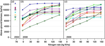
Modellers were not provided with the data on above-ground biomass dynamics. The simulated total above-ground biomass varied considerably among models (Fig. 7). Calibration at fertilizer N rates of 78 kg N/ha in 2002 and 90 kg N/ha in 2008 resulted in a wide range of estimates of total above-ground biomass at maturity, from 5970 kg/ha to 12380 kg DM/ha. APSIM provided generally the highest total above-ground biomass estimates and COUP the lowest.
Modelled total above-ground biomass at physiological maturity (growth stage (GS) 90) in (a) 2002, (b) 2008 and (c) 2009. Models included are APSIM (A), CERES (B), COUP (U), CROPSYSTa (Y), CROPSYSTb (Z), DAISY (D), EPIC (E), FASSET (F), HERMES (H), MONICA (M), STICS (S) and WOFOST (W).

In the test year, simulated total above-ground biomass at maturity at N rate of 90 kg N/ha averaged 8960 kg/ha (s.d. = 1673 kg/ha) across all models, and this was close to the observed total above-ground biomass of 7560 kg DM/ha (s.d. = 1476 kg/ha). There was a wide range between the models, from 5980 to 10950 kg/ha. The three lowest estimates were from COUP, EPIC and CROPSYSTa, and the three highest were from FASSET, DAISY and APSIM.
All models increased their total above-ground biomass with increasing N rates. In 2008, N rate from 0 kg/ha to 150 kg/ha increased total above-ground biomass 27 kg DM/kg N (s.d. = 11·5 kg DM/kg N) and in 2009 64 kg DM/kg N (s.d. = 10·4 kg DM/kg N) when averaged over all models.
Maximum root biomass estimates ranged from 500 kg/ha of CERES to 3220 kg/ha in EPIC (Fig. 8), while the maximum root biomass estimates were not available from APSIM, CROPSYSTa and STICS. Root biomass estimates of other models except for CROPSYSTb responded to N fertilization with increasing biomass with increasing N rate. Steepest responses were given by COUP, EPIC and FASSET (Fig. 8).
Modelled root biomass at physiological maturity (growth stage (GS) 90) in (a) 2002, (b) 2008 and (c) 2009. Models included are CERES (B), COUP (U), CROPSYSTb (Z), DAISY (D), EPIC (E), FASSET (F), HERMES (H), MONICA (M) and WOFOST (W).

Harvest index
In most models, harvest index (HI) estimates ranged from 0·4 to 0·6 (data not shown), which is plausible when compared with figures reported for spring cereals in Finland (Peltonen-Sainio et al. Reference Peltonen-Sainio, Muurinen, Rajala and Jauhiainen2008) or the observation of 0·6 in 2009 harvest of N90. The only models that were out of this range were COUP with HI as high as 0·7 and APSIM with low HI of 0·3. COUP, STICS and WOFOST were the only models that estimated a slight decrease in HI with increasing N rates.
DISCUSSION
Overall model performance in estimating yield response to Nitrogen
Previous model comparisons have shown that minimal calibration of crop models can lead to a high degree of uncertainty of yield estimates (Palosuo et al. Reference Palosuo, Kersebaum, Angulo, Hlavinka, Moriondo, Olesen, Patil, Ruget, Rumbaur, Takac, Trnka, Bindi, Caldag, Ewert, Ferrise, Mirschel, Saylan, Siska and Rötter2011; Rötter et al. Reference Rötter, Palosuo, Kersebaum, Angulo, Bindi, Ewert, Ferrise, Hlavinka, Moriondo, Nendel, Olesen, Patil, Ruget, Takac and Trnka2012; Asseng et al. Reference Asseng, Ewert, Rosenzweig, Jones, Hatfield, Ruane, Boote, Thorburn, Rötter, Cammarano, Brisson, Basso, Martre, Aggarwal, Angulo, Bertuzzi, Biernath, Challinor, Doltra, Gayler, Goldberg, Grant, Heng, Hooker, Hunt, Ingwersen, Izaurralde, Kersebaum, Mueller, Naresh Kumar, Nendel, O'Leary, Olesen, Osborne, Palosuo, Priesack, Ripoche, Semenov, Shcherbak, Steduto, Stöckle, Stratonovitch, Streck, Supit, Tao, Travasso, Waha, Wallach, White, Williams and Wolf2013). The current study shows that more detailed data provided for model calibration does not necessarily result in high accuracy of model simulations when the models are applied to new situations, in particular when simulations are done for sub-optimum management such as N-limited growth, and for environmental conditions that deviate strongly from the calibration conditions, as in the current study. The RMSE values of grain yield were three times higher in test year 2009 compared with calibration year 2008. Interesting topics for future research are how sensitive the model-estimated yield responses are to the selected calibration data and its quality, and to what extent model results can be extrapolated to new situations, beyond the environmental ‘data space’ of the calibration years.
It was decided to use years for model calibration and testing in chronological order, which is a typical set-up for modelling studies including model calibration and projections for future. The selected years most likely affected the simulated N responses as the yield response to N fertilizer was very different between the years. In further studies, it would be useful to avoid unnecessary restrictions dividing experimental years between calibration and testing. Furthermore, testing the sensitivity of the modelling results on different calibration and test years could also be a useful addition in future modelling studies.
Despite the problems of the individual models to maintain their good performance from calibration to test year, the MMM yield response to N matched well with observations; only three models had lower RMSE (380–580 kg/ha) in 2009 than MMM (590 kg/ha). The MMM relies on the assumption that results of a large group of models will converge close to the ‘true value’, mainly by error compensation, while the most accurate models might become scaled back to average (Knutti Reference Knutti2010; Asseng et al. Reference Asseng, Ewert, Rosenzweig, Jones, Hatfield, Ruane, Boote, Thorburn, Rötter, Cammarano, Brisson, Basso, Martre, Aggarwal, Angulo, Bertuzzi, Biernath, Challinor, Doltra, Gayler, Goldberg, Grant, Heng, Hooker, Hunt, Ingwersen, Izaurralde, Kersebaum, Mueller, Naresh Kumar, Nendel, O'Leary, Olesen, Osborne, Palosuo, Priesack, Ripoche, Semenov, Shcherbak, Steduto, Stöckle, Stratonovitch, Streck, Supit, Tao, Travasso, Waha, Wallach, White, Williams and Wolf2013; Carter Reference Carter2013: Martre et al. Reference Martre, Wallach, Asseng, Ewert, Jones, Rötter, Boote, Ruane, Thorburn, Cammarano, Hatfield, Rosenzweig, Aggarwal, Angulo, Basso, Bertuzzi, Biernath, Challinor, Doltra, Gayler, Goldberg, Grant, Heng, Hooker, Hunt, Ingwersen, Izaurralde, Kersebaum, Müller, Naresh Kumar, Nendel, O'Leary, Olesen, Osborne, Palosuo, Priesack, Ripoche, Semenov, Shcherbak, Steduto, Stöckle, Stratonovitch, Streck, Supit, Tao, Travasso, Waha, White and Wolf2015). The current results show that MMM cannot always effectively correct systematic errors in model simulations. For instance, as shown by Rötter et al. (Reference Rötter, Palosuo, Kersebaum, Angulo, Bindi, Ewert, Ferrise, Hlavinka, Moriondo, Nendel, Olesen, Patil, Ruget, Takac and Trnka2012) for a small ensemble (<10) of crop models, due to poor calibration an extreme outlier model can result in a less robust estimate by MMM. In such cases, using the multi-model median could provide a better estimate (Martre et al. Reference Martre, Wallach, Asseng, Ewert, Jones, Rötter, Boote, Ruane, Thorburn, Cammarano, Hatfield, Rosenzweig, Aggarwal, Angulo, Basso, Bertuzzi, Biernath, Challinor, Doltra, Gayler, Goldberg, Grant, Heng, Hooker, Hunt, Ingwersen, Izaurralde, Kersebaum, Müller, Naresh Kumar, Nendel, O'Leary, Olesen, Osborne, Palosuo, Priesack, Ripoche, Semenov, Shcherbak, Steduto, Stöckle, Stratonovitch, Streck, Supit, Tao, Travasso, Waha, White and Wolf2015). Yet, if all the models are (systematically) wrong, as seems to have occurred for estimating LAI in the unfertilized plot in 2009, then the multi-model median will not help. In 2009, all models clearly over-estimated maximum LAI for the N0 plot in 2009. According to the laws of light extinction of leaf canopies, light interception, resulting assimilation, etc., a maximum LAI of 1·5 can at most intercept 0·60 of the light of a canopy with max LAI of 3·0 (de Wit Reference de Wit1965; Goudriaan Reference Goudriaan1977). Hence, the much lower control yield in 2009 as compared with 2008 and 2002 was to be expected – but all models failed to reproduce observed values. This also clearly calls for in-depth studies to improve models in terms of simulating the dependence of leaf area development on temperature and N availability. Thus, in the current case, due to severe systematic errors in modelling LAI under cold temperatures and low N, the MMM was not able to represent the specific differences of the 2 years either.
Observed differences in yield responses to N between the seasons 2008 and 2009 were quite large even though soil data and weather conditions that were converted to model input did not show large differences. Reasons for these discrepancies could be related to the different ways the models apply to estimate maximum yield and soil N supply.
Maximum yield with optimal N was 20% higher in 2009 than in 2008 and most models under-estimated that response. None of the main factors that have been found to have negative effects on barley yields in Finland, such as early summer drought, excessive rain early in the season, high temperatures around heading or accelerated temperature sum accumulation rates during a period of 2 weeks before heading (Hakala et al. Reference Hakala, Jauhiainen, Himanen, Rötter, Salo and Kahiluoto2012), were markedly different in 2009 as compared with 2008. Yet there are a number of other adverse weather events that can have a considerable yield impact in a particular year (Van Oort et al. Reference Van Oort, Timmermans, Meinke and van Ittersum2012; Rötter et al. Reference Rötter, Höhn, Trnka, Fonzek, Carter and Kahiluoto2013).
After careful re-analysis of the weather data, one adverse weather event was found in the calibration year 2008 and one positive weather event in test year 2009 that can partly explain the difference in observed maximum yields between the 2 years. In 2008, there was heavy rainfall during the last phase of grain filling, which may have led to yield penalties. Although direct grain losses were not reported, the intensive rainfall event may have caused water-saturated soil conditions and interfered with grain filling. Modelled soil water contents increased in all models after heavy rainfall at the beginning of August, but soil water content increased above field capacity only in APSIM and COUP.
In 2009 the positive weather event that resulted in early and vigorous tillering was low daily average temperature after emergence. The observed number of tillers was clearly higher than the reported common value of 1·3 in two-row barley in Finland (Peltonen-Sainio et al. Reference Peltonen-Sainio, Jauhiainen, Rajala and Muurinen2009). Heads and grains of tillers developed early enough to produce sufficient individual grain size as can be seen from grain weight of 2009. Under northern conditions, grains on side tillers mature later but tillering enhances grain yield especially in two-row barley cultivars (Peltonen-Sainio et al. Reference Peltonen-Sainio, Jauhiainen, Rajala and Muurinen2009). The number of productive tillers has been noted to increase with moist conditions during early growth (Mäkelä & Muurinen Reference Mäkelä and Muurinen2012) and with high N rates and cool conditions delaying maturity (Peltonen-Sainio et al. Reference Peltonen-Sainio, Jauhiainen, Rajala and Muurinen2009). Enhanced tillering increased number of grains and growing conditions were sufficient to increase yield potential. Tillering is not explicitly included in process descriptions of any of the models and this effect was not covered by them indirectly either.
The avoidance or enhancement of stresses caused by drought, diseases, pests, nutrients (other than N), etc. is necessary when modelling N-limited growth. In the current study, disease and pest stresses were ruled out by excluding such years and treatments according to the observations. Considering soil water contents, water deficits cannot be ruled out with certainty. More exact measurements from plots with diverging N rates, to cover possible water shortages in high-yielding treatments, would have been useful to clarify this.
Models were calibrated against the relatively high yield of the N0 treatment in 2008. In 2009, unfertilized grain yield was 40% lower and grain N uptake was 26 N kg/ha lower compared with 2008. Soil characteristics provided to modellers for estimating soil N mineralization were few, including only initial soil C and N concentrations. Soil and weather input did not reveal any clear reason for differences in observed soil N supply between 2008 and 2009. Neither weather conditions in previous winters or pre-sowing in spring revealed any major differences. Detailed simulation results of most models showed that in 2009 soil water content in 0–30 cm at 40–60 DAS was lower than in 2008, which indicates a short period of possible water stress. Information on soil N mineralization was checked from three models: MONICA and STICS provided higher N mineralization in 2008 (63 and 60 kg N/ha) than in 2009 (49 and 40 kg/N ha) from sowing to harvest; COUP on the other hand, showed lower soil moisture content in 2009 than in 2008, but it did not affect the soil N mineralization simulated by the model. Observations of N leaching in a nearby field showed a small leaching event of 3 kg N/ha on 6 June 2009, which could also partly increase the difference of N supply between the years 2008 and 2009. Unknown effects of short water stress periods, leaching events and soil N mineralization are possible causes of different yield responses to N rate between calibration and test year.
Modelling nitrogen dynamics
It appears that the level of detail in process description of N dynamics in soil and plant was not a major factor affecting the different performance of the models. For example, WOFOST with its relatively simple approach using soil N supply estimates based on target yields did not show remarkably weaker performance in comparison with models with more detailed N processes and several soil organic matter pools such as COUP or EPIC. This raises the question of whether, more generally, the models considered in the current study are capable of predicting N processes sufficiently accurately without site-specific calibration as is assumed in many model applications. In the current study, model parameterizations were not compared as models differ widely in their process descriptions. However, an interesting continuation of the study would be to examine calibration effects on simulated responses of multiple models for soil N mineralization, LAI, N uptake, etc. and a wider range of conditions.
Barley yields for treatments without N fertilization varied in the current study and they generally seem to vary considerably across non-fertilized sites in Finland (Valkama et al. Reference Valkama, Salo, Esala and Turtola2013). The main parameters affecting N supply of unfertilized plots are N mineralization from crop residues and soil organic matter. Microbial turnover of C and N, and its interaction with the crop, has long been recognized as a key process for N supply (Kersebaum et al. Reference Kersebaum, Hecker, Mirschel, Wegehenkel, Kersebaum, Hecker, Mirschel and Wegehenkel2007). Simulation of soil N supply, however, requires adequate long-term information of the cultivation history of the site (Petersen et al. Reference Petersen, Schjønning, Olesen, Christensen and Christensen2013), since soil organic matter model pools cannot usually be measured directly.
According to Hay & Porter (Reference Hay and Porter2006) the main effects of N shortage are found in the plant canopy and expressed by lower shoot numbers, smaller leaves and faster leaf and shoot death. Indeed, field observations showed clear reduction in LAI caused by low N rates. One would thus assume that the models that perform best in their LAI estimations with all N rates, APSIM, CERES and FASSET, would also produce best estimates of DM yield. However, they did not perform better than other models. Furthermore models differed considerably in their evaluations of total above-ground and root biomasses. In future studies, the differences between the models in their total biomass accumulation and allocation should be studied closely.
Sources of uncertainty
The current study shows, like the few comparable studies (Diekkrüger et al. Reference Diekkrüger, Söndgerath, Kersebaum and McVoy1995), that the same exercise for the same model carried out by different teams can provide very different results. The two CROPSYST teams in the current study applied different model versions (e.g. using two fundamentally different soil water balance routines) and calibration approaches that yielded very different model estimates for yields and other variables. This further emphasizes the important role of calibration for the model results. Model inter-comparisons are thus comparisons of case-specific model realizations and their results cannot easily be generalized.
When calibrating yield response to N rate, the good calibration of unfertilized yield and its N uptake is essential in order to estimate soil N mineralization exactly. In calibration, grain yields of N0 differed from 1780 to 3540 kg/ha among the models, and their total above-ground N uptakes of N0 ranged from 30 to 90 kg/ha. On the other hand, it must be kept in mind that the need of detailed calibrations reduces the generality and possibilities to apply crop models. For instance, if one would force the model to reproduce yield at N0 accurately, this might completely distort its capability to reasonably estimate the yield response curve to increasing N rate. Smith et al. (Reference Smith, Smith, Powlson, McGill, Arah, Chertov, Coleman, Franko, Frolking, Jenkinson, Jensen, Kelly, Klein-Gunnewiek, Komarov, Li, Molina, Mueller, Parton, Thornley and Whitmore1997) stated that the level of site-specific calibration was one of the main reasons for differences of soil organic matter model performances. They also stated that before models can be used in a truly predictive manner their ability to predict soil organic carbon dynamics without site specific calibration should be improved. For modelling yield response to N fertilizers it would help to have the indigenous soil N supply capacity as an input, as used in Setiyono et al. (Reference Setiyono, Yang, Walters, Dobermann, Ferguson, Roberts, Lyon, Clay and Cassman2011), and then the weather impact on soil N mineralization and N loss processes should be dealt with by the model.
Although it is challenging to parameterize the size and kinetics of different soil organic N pools of the models (Ros et al. Reference Ros, Hanegraaf, Hoffland and van Riemsdijk2011; Dessureault-Rompré et al. Reference Dessureault-Rompré, Zebarth, Burton, Gregorich, Goyer, Georgallas and Grant2013), these would be needed in a detailed calibration. Measurement of soil N mineralization potential, which could show the availability from organic N under optimal conditions, is one measure that would support modelling of N mineralization. However, soil N dynamics and mineralization potential show high spatial variability even within uniformly managed fields (Baxter et al. Reference Baxter, Oliver and Gaunt2003; Kersebaum et al. Reference Kersebaum, Lorenz, Reuter, Schwarz, Wegehenkel and Wendroth2005) and data sets of the different seasons are not observed at exactly the same locations. Therefore, measurements of soil mineral N during the growing season under the different N treatments would have been very useful for both model calibration and testing. Additionally, data on N fluxes (atmospheric and leaching losses) would have been helpful to better quantify N availability for crop uptake. Since soil moisture and temperature greatly affect soil N mineralization, the models should be accurate in modelling soil water and temperature dynamics. In particular, the need for better understanding of soil moisture and temperature interactions has been raised due to the task of soil N modelling under different climate change scenarios (Guntinas et al. Reference Guntinas, Leiros, Trasar-Cepeda and Gil-Sotres2012; Novem Auyeung et al. Reference Novem Auyeung, Suseela and Dukes2013). A major challenge is therefore to develop robust procedures for parameterizing the models with the relatively sparse data available for soil input at larger scales. This cannot be addressed without properly designed and representative field experiments conducted over sufficient climatic and soil gradients.
To improve the predictive capacity of the models under a wide range of environmental conditions, there still seems to be a need for better understanding and description of the fundamental processes in the various crop-soil-atmosphere sub-systems (i.e. associated modules or routines). This was illustrated in the current study in particular for modelling leaf area development under colder temperatures and low N. When using crop models to project effect of different N fertilizer rates, coupling a crop model with various soil modules, soil N mineralization, soil water and temperature fluxes and crop growth is essential. Particularly, crop models tend to have completely different assumptions about N supply from soil that can lead to high uncertainty when soil N supply can provide a considerable share of crop N demand. In order to improve modelling of various soil processes and crop N uptake, very detailed experimental data sets from a wide range of climate and soil conditions would be needed. Therefore it is suggested that relevant institutes should organize field experiments on at least two comparable soil types (sand and clay) on different European climate conditions (north, south, west, eastern and central Europe) using one cultivar and the same N doses for at least three seasons. All field experiments should include detailed monitoring of soil water content, soil mineral N content and plant biomass accumulation in addition to yield and N uptake measurements. Finally, modellers should also put more emphasis on automatic calibration procedures to decrease the effect of human error on the calibration process.
The authors wish to acknowledge the financial assistance provided under the umbrella of COST action 734 ‘Impacts of Climate Change and Variability on European Agriculture (CLIVAGRI)’ and the work of individual researchers was funded by various bodies: T. Palosuo, T. Salo and R. Rötter, the strategic project MODAGS funded by MTT Agrifood Research Finland, and projects FACCE MACSUR and NORFASYS (decision nos. 268277 and 292944) funded by the Ministry of Agriculture and Forestry and the Academy of Finland, respectively; K. C. Kersebaum performed parts of the current study under the umbrella of FACCE MACSUR funded by the German Federal Office for Agriculture and Food and COST ES1106; C. Nendel was supported by ZALF in-house funds; J.E. Olesen and R.H. Patil, CRES funded by Danish Strategic Research Council; P. Hlavinka was supported by the Ministry of Education, Youth and Sports of CR within the National Sustainability Program I (NPU I), grant number LO1415; M. Trnka, Crop modelling as a tool for increasing the production potential and food security of the Czech Republic funded by National Agency for Agricultural Research (QJ1310123) and project LD 13030 – Water resources in the Czech Agriculture under the Climate Change conditions - CZECH-AGRIWAT; Mr Antti Ristolainen (2002) and Mr Petri Kapuinen (2008 and 2009) are acknowledged for providing data from their field experiments.