Introduction
Improvement in the production of mechanical engineering products is hampered without the use of new progressive technological processes that enhance the operational lifetime and reliability of components in the most severe operating conditions. In this regard, the methods for surface hardening by laser irradiation, electron and ion beams attract a lot of attention (Proskurovsky et al., Reference Proskurovsky, Rotshtein, Ozur, Ivanov and Markov2000; Bocharov et al., Reference Bocharov, Eletskii, Zakharenkov, Zilova, Sliva, Terentyev, Fedorovich and Churilov2018). The exposure of a high-intensity pulsed ion beam (HIPIB) at gigawatt power level with the energy density of 2–10 J/cm2 provides a rapid heating of the surface layer at a rate of 109 K/s, followed by a fast cooling at a speed of 108–1010 K/s (Bystriskii and Didenko, Reference Bystriskii and Didenko1989). Such treatment of an item makes it possible to obtain in the surface layers compositions and nanoscale structures that are inaccessible to any of the traditional metallurgical methods. As a result, the properties of materials are improved: hardness, strength, wear and corrosion resistance, etc.
The HIPIB composition determines the depth of a modified layer of a treated item and the specific energy release. Therefore, optimizing of the treatment procedure requires to control the composition and the quantitative ratio of the ions in the beam. In metals and alloys with a range of ions (ion energy of 200–300 keV) of <0.5 µm, the thermal front propagates toward the end of the pulse to a depth of 2–4 µm (Pushkarev et al., Reference Pushkarev, Isakova and Khailov2015а). Therefore, for metal products, the composition of HIPIB is not as important as the depth of propagation of the thermal front. However, for a study and optimization of the ion diode operation, it is important to know the composition of the ion beam.
A method for measuring the composition of an ion beam with the acceleration of ions in an electric field and their spatial separation by means of a magnetic field was first proposed by J. Tomson in 1913. In 1920, Aston designed a prototype of a modern magnetostatic mass spectrometer (Aston, Reference Aston1920). To detect ions with a large mass in a Thomson spectrometer, it was necessary to use a magnetic field with an induction of more than 1 T, which complicates the instrument and increases its dimensions and mass. Detailed information on the composition of the beam, the energy spread of ions in the Thomson spectrometer is obtained using the track diagnostics based on CR-39 plastics (Fleischer et al., Reference Fleischer, Price and Walker1965; Cartwright et al., Reference Cartwright, Shirk and Price1978). However, processing of the recording plates requires a lot of time and does not allow for a quick monitoring of the beam parameters. The use of photosensitive semiconductor matrices in the Thomson spectrometer (Kasuya et al., Reference Kasuya, Watanabe, Ido, Adachi, Nishigori, Ebine, Okayama, Funatsu, Sunami, Wu, Hotta and Miyamoto1999) (for recording the spatial separation of ions) is difficult due to destruction of the photosensitive elements in high-voltage sources of HIPIB with a large energy density.
To analyze the HIPIB composition, a phenomenon of spatial separation of different types of ions along the path from the diode to the recording device can be used. When accelerating in the anode–cathode (A–C) gap of the diode, ions of different mass and degree of ionization acquire the same energy, but different speeds. The idea of the time-of-flight mass analyzer belongs to Stephens, who proposed the design of the device in 1946 (Stephens, Reference Stephens1946). The first analyzer was constructed by Wiley and MacLaren (Reference Wiley and MacLaren1955). The advantages of time-of-flight mass analyzers include the high upper threshold of the detected ion mass, limited only by the decrease in the sensitivity of the ion detector. The composition of HIPIB is determined by a time-of-flight method using two ion current sensors placed at different distances downstream from the diode (Moskalev, Reference Moskalev1992). A more detailed review on the history of development of time-of-flight mass spectrometers from the moment of their invention to the present time can be found in Mamyrin (Reference Mamyrin2001).
The use of a high-speed recording device (an ion collector) and a wideband oscilloscope allows the ion beam to be monitored quickly using only one sensor installed at a sufficient distance from the diode. The purpose of this work is the development and testing of a high-resolution time-of-flight technique for operational control of HIPIB composition and the energy spectrum.
Ion beam composition measurement procedure
To analyze HIPIB composition, we used the time-of-flight diagnostics with a collimated Faraday cup (CFC) (Ghadikolaee and Ghadikolaee, Reference Ghadikolaee and Ghadikolaee2012) with magnetic cut-off as a recording device for ions. It was assumed that in the diode, different ions are accelerated synchronously during the accelerating voltage pulse; the concentration of the anode plasma does not limit the ion current density; in the ion drift path from the diode to the CFC, their velocity does not change. The density of the ion beam usually does not exceed 1012 cm−3, so the probability of ion collisions (and changes of their velocity) in the drift region is negligible.
The signal at the CFC is delayed due to the time required for ions to travel from the diode to the device. The delay is
 $${\rm \Delta} t = \displaystyle{D \over {v_{\rm i}}},$$
where D is the distance from the CFC to the diode, v i = const is the ion velocity in the drift region.
As an ion passes through the A–C gap, it acquires kinetic energy equal to
 $$E = \displaystyle{{m_{\rm i} \times v_{\rm i}^2} \over 2} = z \times U,$$
where m i and z are the mass and charge of an ion, respectively, and U is the accelerating voltage.
From Eqs. (1) and (2), we obtain an equation for calculating the arrival delay of ions to the CFC:
 $$\Delta t = D\left( {\displaystyle{{m_{\rm i}} \over {2zU}}} \right)^{1/2}.$$
In the space-charge limitation regime and in non-relativistic approximation, taking into account the plasma expansion across A–C gap, the ion current density in the diode is described by (Langmuir, Reference Langmuir1913)
 $$j(t) = \displaystyle{{4K{\rm \varepsilon} _0\surd (2z)} \over {9\surd m_{\rm i}}} \times \displaystyle{{U^{3/2}} \over {{(d_0 - vt)}^2}},$$
where d 0 is the initial A–C gap spacing, ε0 is the absolute permittivity, v is the plasma expansion velocity, and K is the ion current amplification coefficient.
Equations (3) and (4) were used to model the signal profile from the CFC. For each instant of the voltage applied to the diode (0.4 ns step), we calculated the current density of a certain type of ions and the delay in the arrival of these ions to the CFC. The calculated curves were compared with the experimental data. Such a technique allows for a more accurate determination of HIPIB composition than that described by Furman et al. (Reference Furman, Stepanov and Furman2007). The plasma expansion velocity (1.2–1.6 cm/μs) was determined from the diode impedance by a method described by Pushkarev et al. (Reference Pushkarev, Isakova and Khailov2014).
Time-of-flight diagnostic testing at different diodes
A barrel diode
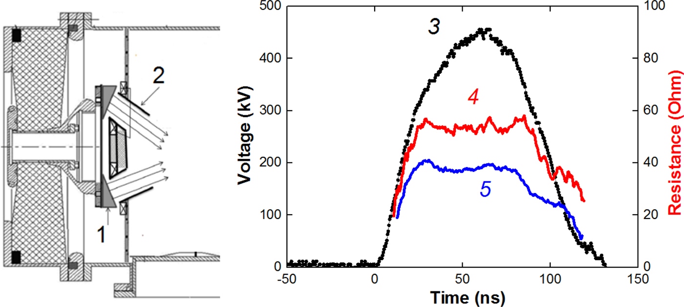
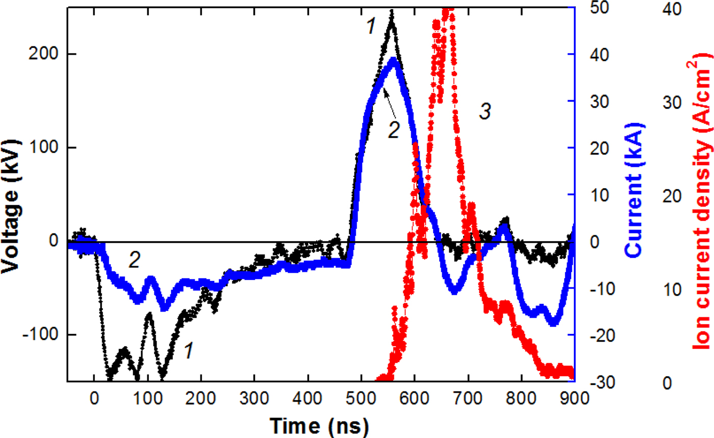
The time-of-flight diagnostics was used to analyze the composition of HIPIB formed by a focusing diode with a dielectric anode and radial external magnetic field (barrel diode) at the BIPPAB-450 accelerator (Xiao et al., Reference Xiao, Shen, Qu, Liu, Zhong, Zhang, Zhang, Yan, Zhang, Zhang and Le2015; Yu et al., Reference Yu, Liu, Shen, Isakova, Zhong, Zhang, Yan, Zhang, Zhang and Le2017). The accelerator consists of a capacitor storage, a pulsed transformer, and a double forming line (DFL). The output of the DFL is terminated with a step-up transformer, which increases the output of the generator by up to 35 Ω. Figure 1 shows a schematic drawing of the diode connection and characteristic waveforms of the accelerating voltage when operating on a resistive load of 38 or 53 Ω. When generating an ion beam, the diode impedance was matched to the output resistances of the transformer by changing the A–C gap spacing.
Diagram of the diode assembly of the BIPPAB-450 accelerator (1 – anode, 2 – cone cathode), waveforms of voltage (3) and calculated resistance of a load (4–53, 5–38 Ω).

The diode consists of an annular anode and two annular cathodes. The anode is made of a highly conductive material (aluminum) and has radii of 93 mm (external) and 70 mm (internal) and a surface area of 80 cm2. The working surface of the anode contains annular grooves, which are filled with polyethylene. The cathodes are made from stainless steel. The barrel design of the diode provides a closed electrons drift in the A–C gap (Humphries, Reference Humphries1990). The formation of the anode plasma occurs during the breakdown on the dielectric coating surface on the anode (B > B cr) or during ionization of the anode surface by accelerated electrons (B ~ B cr) (Pushkarev et al., Reference Pushkarev, Isakova and Khailov2015а). Background pressure in the vacuum chamber was 0.01–0.03 Pa.
The voltage at the output of the accelerator was measured using a voltage divider that was installed in the transition chamber between the step-up transformer and the diode. The current at the output was measured using a Rogowski coil. The ion current density was determined by a CFC with magnetic cut-off of electrons (B = 0.4 T). Electric signals from the sensors were recorded with a Tektronix 2024B oscilloscope (200 MHz, 5 × 10⁹ readings/s). The synchronization error of electrical signals did not exceed 1 ns. The calibration of the diagnostic equipment showed that it correctly reflects the operation of the accelerator in the short-circuit mode and when operating on a resistive load of 35–55 Ω (voltage 400–450 kV). The accuracy of measurement of voltage, total current of the diode, ion current density, and the frequency characteristics of the diagnostic equipment allows us to calculate the impedance of the diode and the parameters of the ion current with an error of not worse than ±10%.
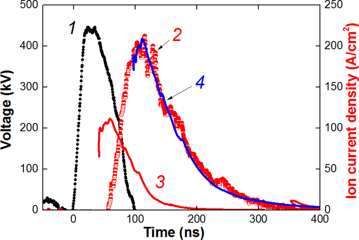
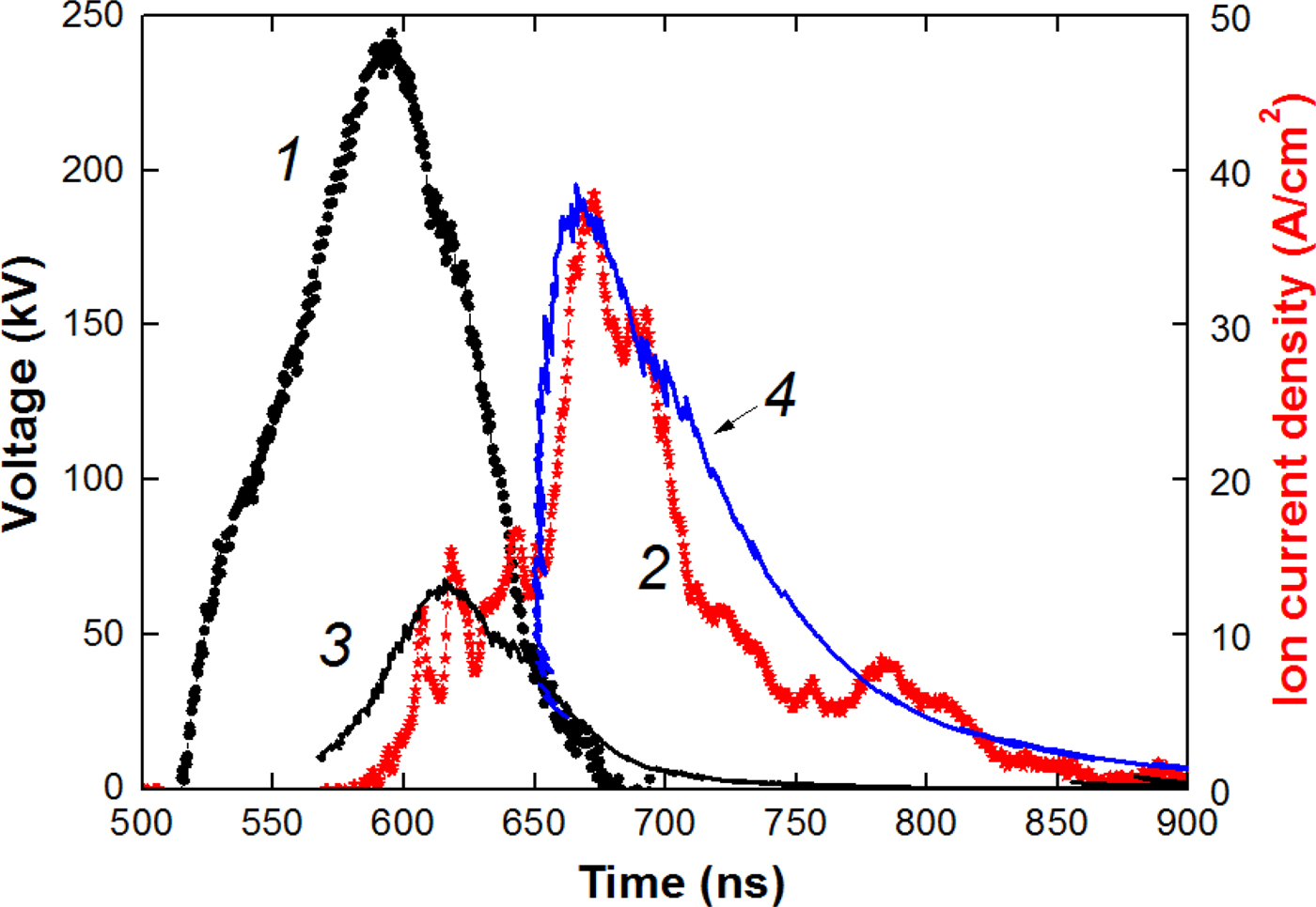
In the first set of experiments, the A–C gap spacing was 6.8 mm, the magnetic induction was 0.6 T at a critical magnetic induction of 0.30–0.32 T. It is found that the ion beam formed by the barrel diode at B > B cr is mainly composed of C+ carbon ions (see Fig. 2).
Waveforms of voltage (1) and ion current density (2, points). Curve 3 is the calculated current density of protons; curve 4 is the calculated current density of C+.
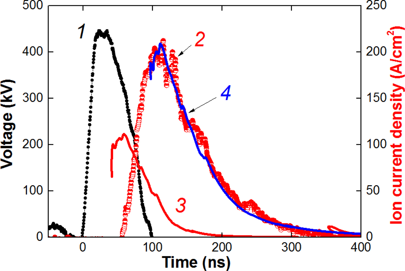
Measurement of the ion current density was carried out with the CFC, installed at a distance of 20 cm downstream from the diode, in the diode focus. Therefore, the ion current density calculated by Eq. (4) was increased (K = 6–10 for different regimes).
Time-of-flight diagnostics allows to determine the duration of anode plasma formation. Calculation of the proton current density was made for the beginning of the accelerating voltage pulse. However, the Faraday cup registered the appearance of the ion current only 10–15 ns after the plotted curve for protons (see Fig. 2). This delay corresponds to the duration of the formation of a continuous plasma layer on the anode.
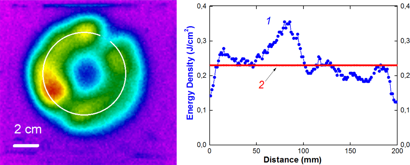
The correctness of the time-of-flight diagnostics for the barrel diode was verified with the thermal imaging diagnostics (Davis et al., Reference Davis, Bartsch, Olson, Rej and Waganaar1997; Isakova and Pushkarev, Reference Isakova and Pushkarev2018). The calculated HIPIB energy density is equal to the product of the accelerating voltage integral over the calculated ion current density (Eq. 4 at K = 1):
 $$\eqalign{q_{{\rm calc}}(t) & = \int {U(t)} \times J_{{\rm ion}}(t)dt \cr \quad & = \displaystyle{{4{\rm \varepsilon} _0\sqrt {2z}} \over {9\sqrt {m_{\rm i}}}} \int {\displaystyle{{U^{5/2}(t)dt} \over {{(d_0 - v \times t)}^2}}} ;\quad {\rm J/c}{\rm m}^2.} $$
Figure 3 shows the thermal pattern of the beam at the target and the distribution of the energy density. The 50 µm stainless steel target was placed 10 mm downstream from the cathode. Each infrared (IR) image was obtained for one accelerator shot.
Infrared image of the beam on the target, distribution of the beam energy density over the circle (1) and calculated energy density of C+ ions (2).

The IR image of the beam was recorded through an exit window located on the flange of the diode chamber. A calcium fluoride (CаF2) or BaF2 parallel-sided plate was used as a window. This window features incomplete transmission in the spectral range of the IR-camera (7–14 µm); therefore, readouts of thethermal imager that records the temperature through the window differ from the actual temperature on the target. The IR-diagnostic equipment was calibrated before the experiments (Isakova and Pushkarev, Reference Isakova and Pushkarev2018 and references therein).
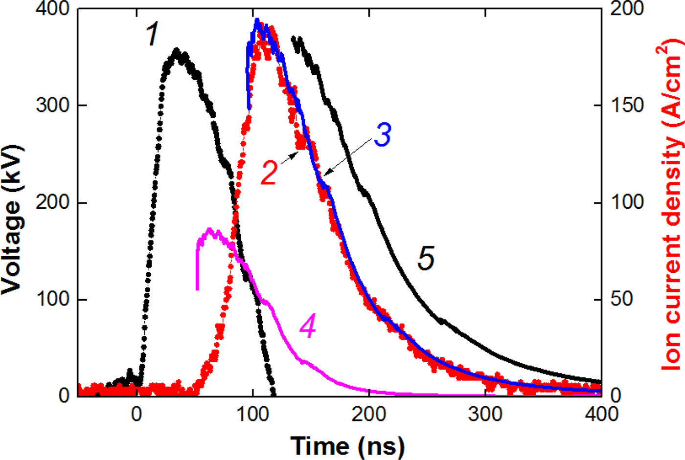
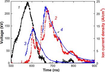
With a decrease in the magnetic induction in the A–C gap to a value close to the critical magnetic induction (0.34–0.37 T), the mechanism for the anode plasma formation and the composition of the ion beam changed. Figure 4 shows the results of time-of-flight diagnostics of HIPIB composition.
Waveforms of voltage (1) and ion current density (2, points). Curve 3 is the calculated current density of C2+ ions; curve 4 is the calculated current density for protons; curve 5 is the calculated current density of C+.

In this diode operation regime, in addition to an increase in the HIPIB energy density, we found an increase in the degree of ionization of carbon ions and a significant reduction in the delay time before formation of the anode plasma. In some experiments, we observed the appearance of triply ionized carbon ions. Therefore, in this mode, the formation of the anode plasma is not only due to the flashover of the anode surface coated with an insulator, but also due to the ionization of the surface material of the anode with accelerated electrons.
A low content of protons in the ion beam formed by a diode with a dielectric anode is associated with a degradation of the dielectric surface because of a prolonged operation of the diode (Zhu et al., Reference Zhu, Dong, Han, Xin and Lei2007). In the dielectric surface breakdown, the thermal decomposition of the organic coating of the anode and carbonization of the near-surface layer take place. The operating life of a diode with a dielectric coating does not exceed 300–400 pulses.
An ion diode with external magnetic insulation of electrons
Time-of-flight diagnostics was also tested at the TEMP-6 accelerator when operating in a single-pulse mode with a diode with a dielectric anode and external magnetic insulation of electrons (Xin et al., Reference Xin, Zhu and Lei2011; Zhu et al., Reference Zhu, Lei, Dong and Ma2003). The anode and cathode have a form of half cylinders to focus the HPIB. The radii of the anode and cathode were 15 and 14 cm, respectively; the slits with dimensions of 0.5 cm × 5 cm were cut out in the working part of the cathode; its transparency was 65%. A perforated polyethylene coating (holes with a diameter of 1 mm) with dimensions of 22 cm × 10 cm and a thickness of 3 mm was fixed on the working surface of the anode. To improve the generation and HIPIB-transport stability, a special cathode design was used. It was divided into two parts, one of which was placed near the front (working) side of the anode, while the other was placed near the back side. The magnetic field was created during the current flow (100 kA, 40 µs) from the external source through the rear electrode of the cathode. This magnetic field propagated into the working A–C gap, thus providing an induction of 0.4–0.8 Т. Owing to the skin effect on the cathode, the magnetic field did not penetrate into the HIPIB transport region, thus providing a forceless drift and efficient focusing of ions.
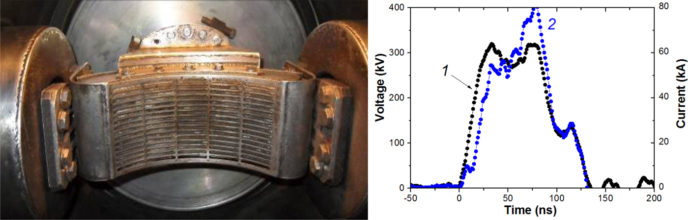
Figure 5 shows a picture of the diode and characteristic waveforms of voltage and current. In this ion diode design, an anode plasma is formed from the breakdown of the dielectric anode surface (B > B cr).
A photograph of a focusing strip diode with external magnetic insulation and an open electron drift. Waveforms of the accelerating voltage (1) and total diode current (2).

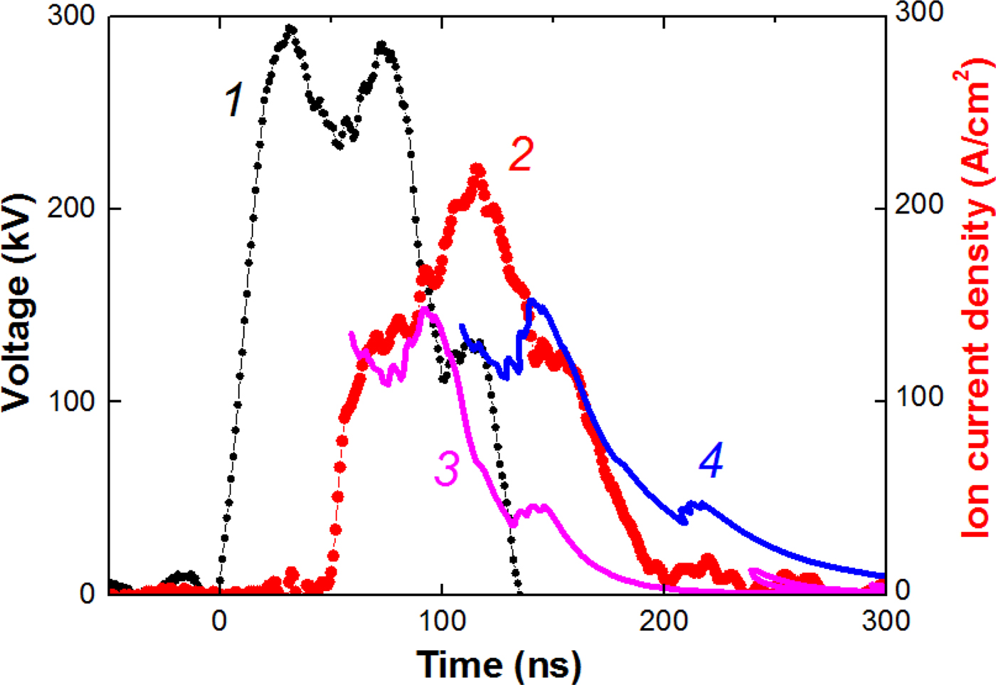
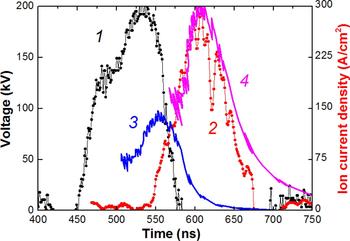
Figure 6 shows the results of time-of-flight diagnostics of HIPIB composition.
Waveforms of voltage (1), ion current density (2, points). Curve 3 is the calculated current density of protons; curve 4 is the calculated current density of C+ ions.

Measurement of the ion current density was carried with the CFC, located at a distance of 15 cm downstream from the diode, in the diode focus. Therefore, the calculated values of the ion current density were increased to account for the focusing of the beam, K H = 7 for protons and K C = 25 for C+ ions for the ion current density in Figure 6.
In the space-charge regime, the ion current density is [see Eq. (4)]:
 $$\displaystyle{{\,j_{\rm H}} \over {J_{\rm C}}} = \displaystyle{{\surd m_{\rm C}} \over {\surd m_{\rm H}}} = \surd 12.$$
Our investigations showed that for an ion beam formed by a dielectric diode with an external magnetic insulation, K C/K H = 3–4; therefore, the ion beam produced by a diode in that regime contains about 50% of protons and 50% of C+ ions.
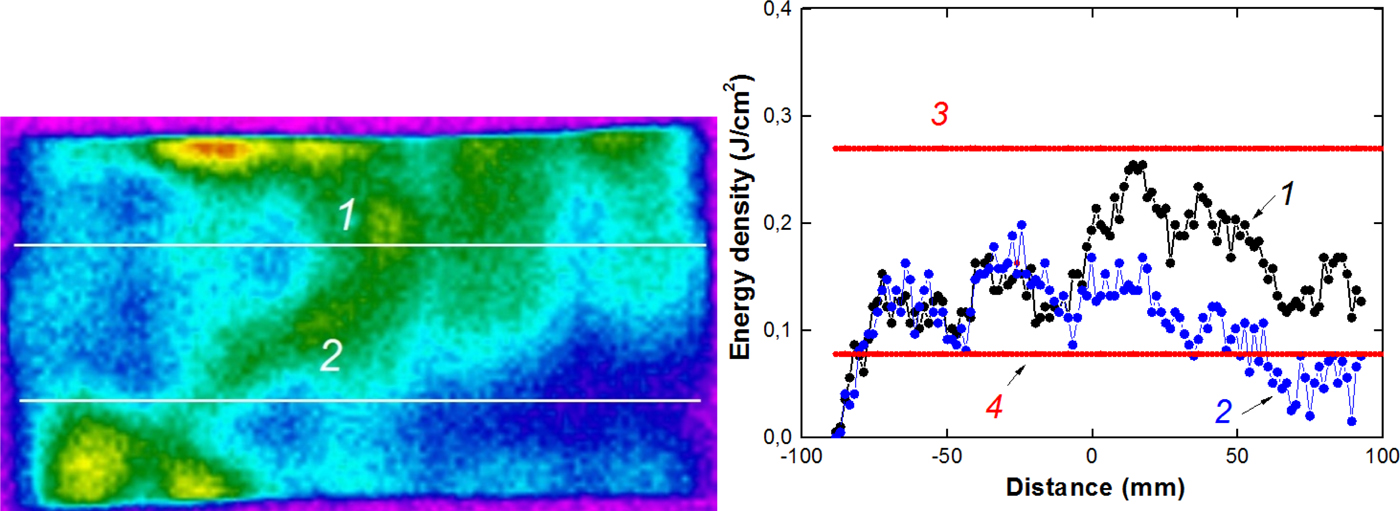
Figure 7 shows the results of thermal imaging diagnostics of an ion beam formed by an ion diode with a dielectric anode in the regime of external magnetic insulation (Zhu et al., Reference Zhu, Lei, Dong and Ma2003). A stainless steel foil of 0.1 mm thick for IR image capture was placed at the output of the cathode, before HIPIB focusing.
HIPIB thermal imprint and the energy density distribution in the upper (1) and lower (2) horizontal sections; the calculated energy density of protons (3) and C+ ions (4).

Figure 7 also shows the calculation of the energy density of an ion beam containing protons or C+ ions calculated from Eq. (5). The performed studies showed that the energy density of HIPIB generated by the diode in the regime of external magnetic insulation, as well as in the barrel diode agree with the calculations.
An ion diode with self-magnetic insulation of electrons
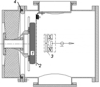
Studies on the HIPIB composition were carried out at the TEMP-4 M (Pushkarev et al., Reference Pushkarev, Isakova and Khailov2015a) accelerator set in the mode of double pulse formation: the first negative pulse (450 ns, 150–200 kV) followed the second positive (150 ns, 200–250 kV). The ion current density on the target is 20–300 A/cm2 for different diodes, the pulse repetition rate is 5–10 pulses/min. The accelerator consists of a capacitive storage (a pulsed voltage generator), a nanosecond pulse generator, and a vacuum diode with self-magnetic insulation of electrons. The nanosecond generator is a coaxial DFL with a liquid dielectric (water) and 4.9 Ω wave impedance. It contains the main and preliminary spark gaps. The block diagram of the diode assembly of the TEMP-4M accelerator is shown in Figure 8.
Schematic representation of the diode assembly: 1 – anode, 2 – cathode, 3 – CFC, 4 – Rogowski coil.

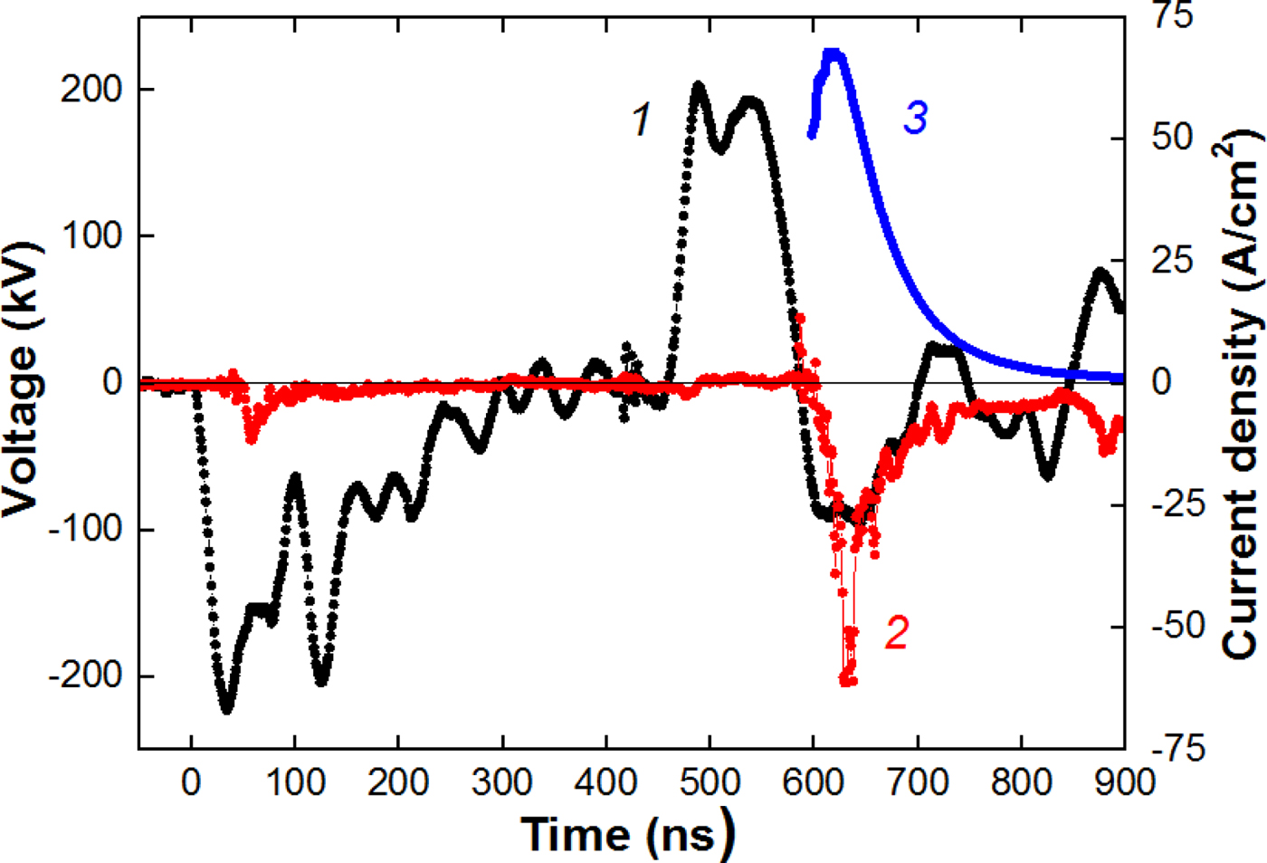
The experiments were performed with a flat diode measuring 20 cm × 4 cm. The anode is made of graphite, and the cathode is made of stainless steel with the slots of 4 mm wide and with an optical transparency of 70%. The A–C gap was selected from the condition of matching the diode impedance with the wave resistance of the DFL; it was 8–9 mm. The strip diode in the mode of self-magnetic insulation effectively works at a pressure of 0.1 Pa with a resource of more than 105 pulses. In the investigated diodes, an explosive electron emission (during the first pulse of negative polarity) is used to form plasma on the anode. Figure 9 shows typical waveforms characterizing the operation of a flat diode with self-magnetic insulation.
Waveforms of accelerating voltage (1), total diode current (2), and ion current density (3). A–C gap spacing of 8 mm; distance to CFC is 18 cm.

The diode current was measured by a Rogowski coil. The ion current density was measured by the CFC with magnetic cut-off of electrons (B = 0.4 T). The voltage at the anode was measured by a high-frequency high-voltage divider installed in front of the diode chamber. Figure 10 shows the waveforms of the accelerating voltage (second pulse) and the density of ion current generated by the planar diode with self-magnetic insulation. The distance from the diode to the CFC is 14 cm.
Waveforms of the accelerating voltage (1) and the ion current density (2, points). Curve 3 is the calculated current density of protons; curve 4 is the calculated current density of C+.

The ion current density was calculated taking into account the plasma erosion effect when the voltage polarity at the anode changes:
 $$j(t) = \displaystyle{{4K{\rm \varepsilon} _0\surd (2z)} \over {9\surd m_{\rm i}}} \times \displaystyle{{U^{3/2}} \over {{\left[ {d_0 - v\,(t - t_0)} \right]}^2}}\;, $$
where t 0 is the moment of polarity change at the anode (t 0 = 450 ns in Fig. 8).
The performed studies showed that HIPIB generated by a flat diode with self-magnetic insulation contains C+ ions (80–85%) and protons. The ion current density is 5–10 times higher than the calculation in Eq. (4). An increased efficiency of ion generation is typical for diodes with self-magnetic insulation (Pushkarev et al., Reference Pushkarev, Isakova and Khailov2015а). The amplification of the ion current density was taken into account in Figure 11 by adding the amplification coefficient K in Eq. (4), the value of which in the calculations was constant during the pulse.
Waveforms of voltage (1) and ion current density (2, points) formed by a flat diode. Curve 3 is the calculated current density of protons; curve 4 is the calculated current density of C+ ions. Distance to CFC is 17 cm.

With increasing the distance from the diode to the CFC, the ion current delay relative to the accelerating voltage increases. In this case, the experimental values of the ion current density and those calculated from (3) and (4) also agree well (see Fig. 11).
We observed that there is no change in the HIPIB composition (during its transport). It confirms the correctness of the time-of-flight technique for the beam compositing measurement.
The developed technique was also tested for a focusing diode with self-magnetic insulation (see Fig. 12). The distance to the CFC is 14 cm.
Voltage waveforms, second pulse (1), ion current density (2, points) in a focusing diode, calculated current density of protons (3) and C+ ions (4).

For the focusing diode, the main part of the ion beam is also composed of singly ionized carbon ions. The current density of C+ ions was calculated taking into account the focusing efficiency. In the used design of the focusing diode, the ion current density was 5–8 times higher than the current density in the flat diode; the ion concentration was (8–10) × 1012 cm−3.
Investigation of the energy distribution of ions
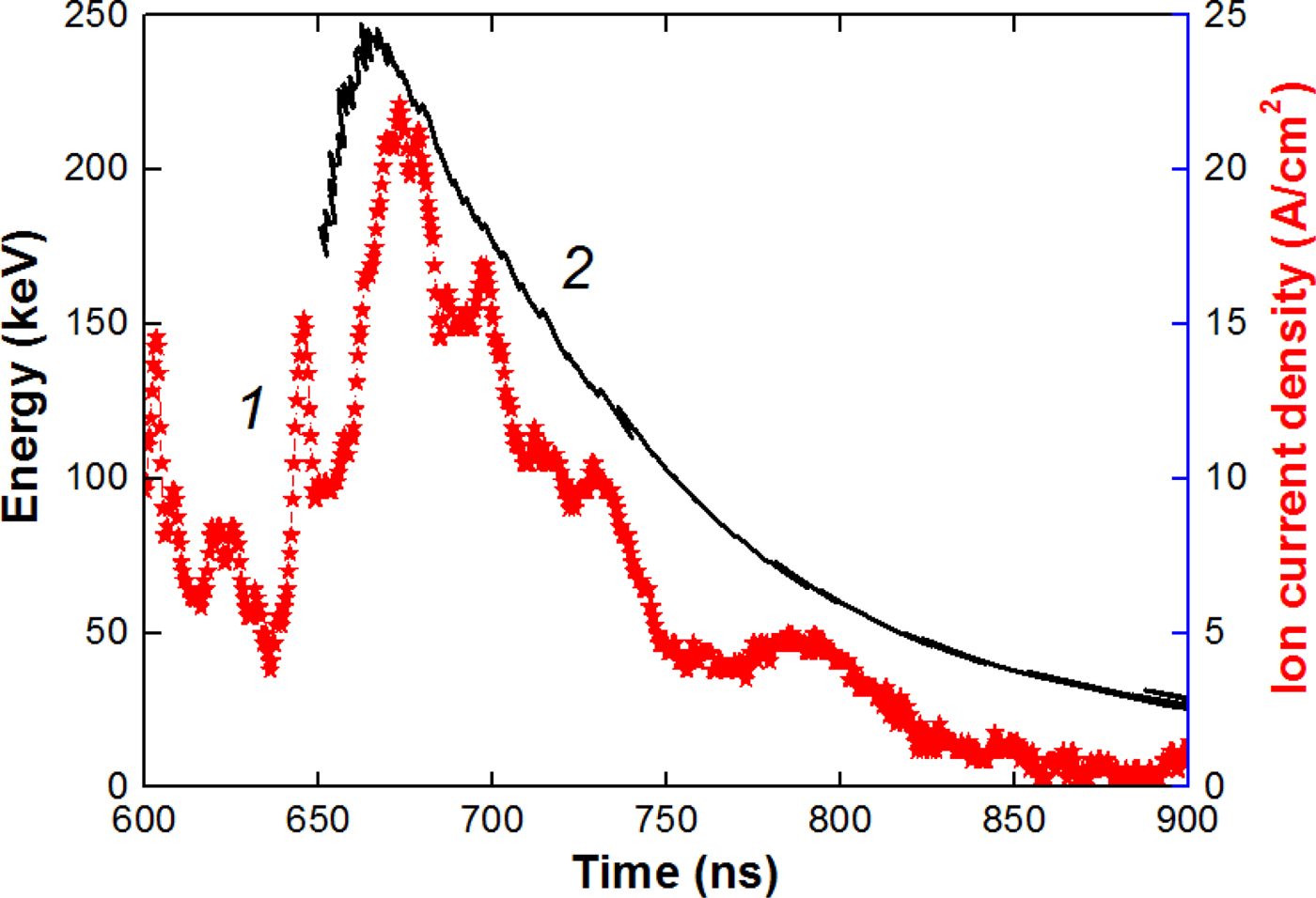
The energy spectrum of ions is one of the most important parameters of HIPIBs, which determines its absorption depth in a target. The developed technique allows for a quick measurement of the energy spectrum separately for each type of ions. In this case, for each value of the accelerating voltage recorded by the oscilloscope (0.4 ns step), we calculated the time delay from Eq. (3) and plotted a curve of the kinetic energy of a certain ion type synchronously with the signal from CFC. Figure 13 shows the calculated values for carbon ions generated by the flat diode (Fig. 8).
Waveforms of the ion current density (1) and the kinetic energy of C+ ions (2).

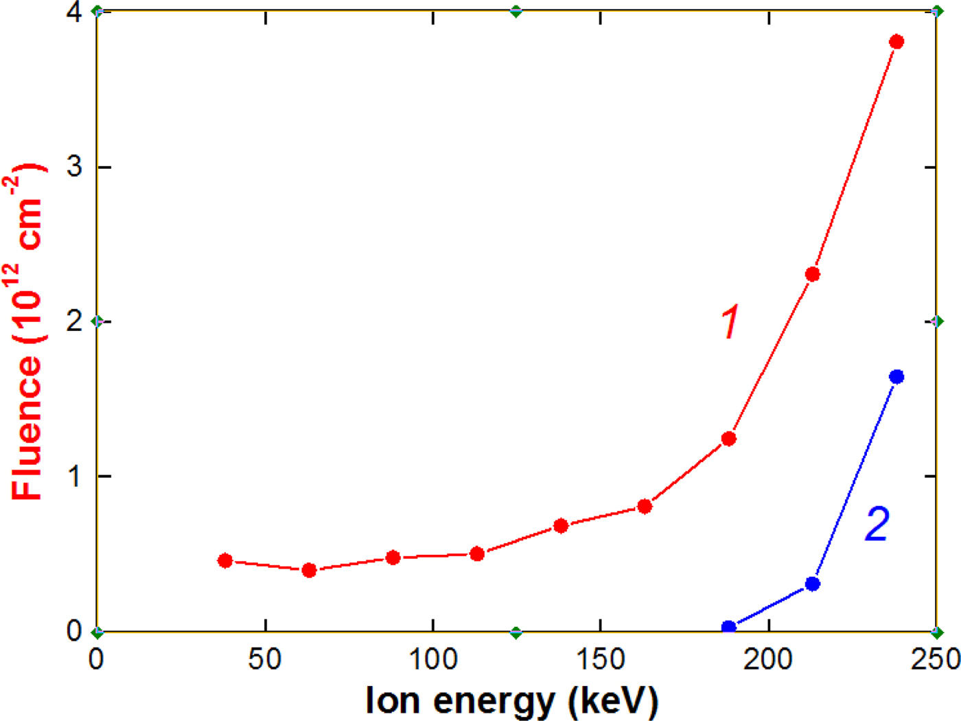
The obtained data make it possible to determine the energy distribution of ions. The energy spectrum of ions formed by the flat diode is shown in Figure 14.
The dependence of the fluence of C+ ions (1) and protons (2) formed by the planar diode on their energy.

The performed studies on the energy spectrum of ions formed by the planar diode with self-magnetic insulation showed that the main part of carbon and proton ions has a kinetic energy of more than 150 keV. The fraction of low-energy ions does not exceed 15–20%. The energy spectrum of an ion beam is determined by the shape of the accelerating voltage pulse. In the TEMP-4M accelerator, we use a Blumlein-nanosecond voltage pulse generator to form a voltage pulse of nanosecond duration. When the impedance of the Blumlein is matched with the load, a voltage pulse of a rectangular-like shape is applied to the load. In such a case, the content of low-energy ions in the beam is low.
Faraday cups
An essential element of the time-of-flight diagnostics is a detector that records ions and measures the ion current. The correctness of its operation largely determines the correctness of the entire diagnostics. To effectively transport and focus the HIPIB, it is necessary to ensure its ion space-charge compensation by low-energy electrons. Otherwise, due to Coulomb repulsion, the ion beam will be spilled.
For measuring the ion beam charge neutralization, we used a Faraday cup without magnetic field or voltage bias. This technique was used by Yatsui et al. (Reference Yatsui, Tokuchi, Tanaka, Ishizuka, Kawai, Sai, Masugata, Ito and Matsui1985). The diameter of the collector was 8 mm, and the diameter of the hole in the lid was 4 mm. The Faraday cup was located at a distance of 14 cm downstream from the diode, in the focus. The Faraday cup is made of a BNC connector. Typical waveforms are shown in Figure 15.
Waveforms of the accelerating voltage (1), neutralized beam current density (2), and calculated current density of С+ ions (3).

The registration time of the neutralized beam current density agrees with the ion current density registration time, which confirms the correctness of measurement of HIPIB space charge.
However, when measuring the ion current density with a Faraday cup, these thermal low-energy electrons must be removed from the beam. For this purpose, a transverse magnetic field (CFC with magnetic cut-off) or a biased electric field (CFC with electric bias) is used. In this section, we present a comparative analysis of the techniques for measuring the parameters of an ion beam with the help of a CFC with a magnetic cut-off and a CFC with an electric bias.
CFC with magnetic cut-off
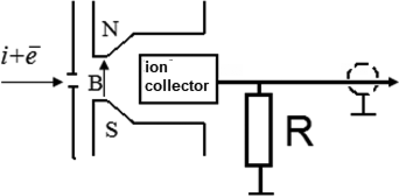
The Faraday cup is designed to measure the current density of charged particles. It is a collector for collecting the charge which is connected to a resistance, and has a collimating hole of a certain diameter, into which the investigated beam particles penetrate and hit the collector. Figure 16 shows a schematic illustration of the CFC structure.
Schematic illustration of the CFC with a transverse magnetic field.

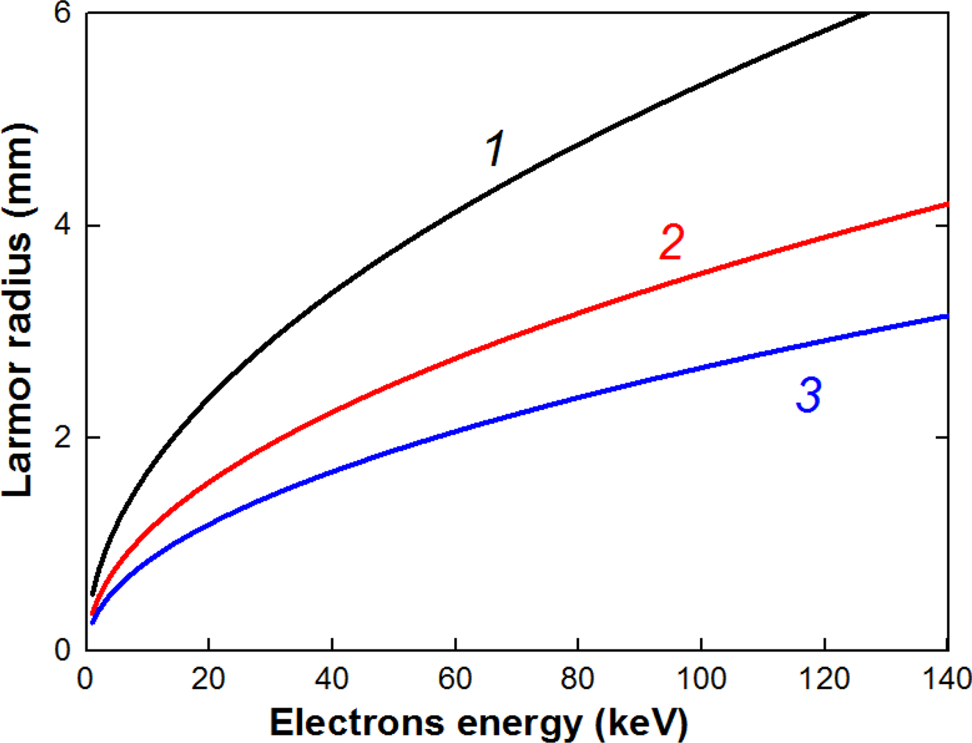
Low-energy electrons that compensate the space charge of the beam ions are deflected in a magnetic field under and do not reach the collector of the CFC. The radius of motion of the electrons in the magnetic field (Larmor radius) is:
 $$R_{\rm L} = \displaystyle{{m \times v} \over {e \times B}} = \displaystyle{{\sqrt {2mE}} \over {e \times B}},$$
where Е = e × U is the kinetic energy of an electron.
Figure 17 shows the dependence of the Larmor radius on the electron energy.
Dependence of the Larmor radius on the electron energy at magnetic induction 0.2 T (1), 0.3 T (2), and 0.4 T (3).

The energy of electrons that compensate the space charge of ions in the beam does not exceed 10 keV and the magnetic field created by a permanent magnet (0.2–0.3 T) is sufficient to prevent the electrons from entering the collector even with a small dimension of the CFC.
Previous studies (Pushkarev et al., Reference Pushkarev, Isakova and Khailov2015b) showed that the skin layer of a neutralized ion beam generated by a diode with an accelerating voltage of 200–300 keV and a current density of more than 100 A/cm2 is 2–3 mm. Therefore, the diameter of the collimating holes in the Faraday cup with magnetic cut-off can be 4–8 mm for effective removal of the low-energy electrons.
CFC with electric bias
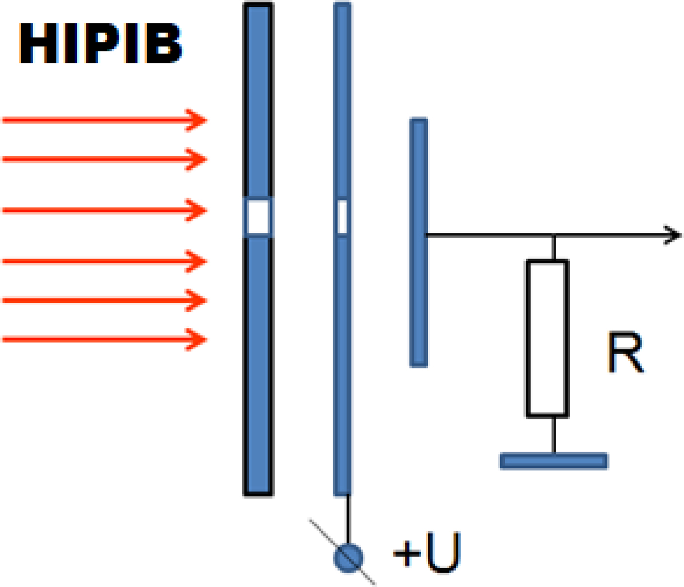
To remove low-energy electrons from the ion beam, a bias electric field in the CFC can also be used. It has an additional metal plate with a collimating hole, at which a voltage of 300–500 V is applied. The polarity of the voltage can be any. Figure 18 shows a schematic illustration of the CFC with electric bias.
Schematic illustration of the CFC with electric bias.

An ion beam, the ion charge in which is compensated by low-energy electrons, is a plasma object that effectively suppresses the penetration of an electric field into its volume. The distance covered by the action of an electric field in the plasma is determined by the Debye radius, which is (Reiser, Reference Reiser2008; Humphries, Reference Humphries1990)
 $$\lambda _{\rm D} = \sqrt {\displaystyle{{\varepsilon _0 \times k \times T} \over {n_{\rm e} \times e^2}}}, $$
where k is the Boltzmann constant and e is the electron charge.
For a HIPIB with singly ionized ions at full charge neutralization, n e = n i. Then the Debye radius, taking into account Eq. (8), is equal to:
 $$\lambda _{\rm D} = \sqrt {\displaystyle{{{\rm \varepsilon} _0kT \times e \times \sqrt {2U \times e}} \over {e^2 \times j \times \sqrt {m_{\rm i}}}}} = \sqrt {\displaystyle{{\sqrt 2 \times {\rm \varepsilon} _0kT} \over {\sqrt {e \times m_{\rm i}}}}} \times \displaystyle{{U^{1/4}} \over {\sqrt j}}. $$
The Debye radius for HIPIB consisting of C+ ions is:
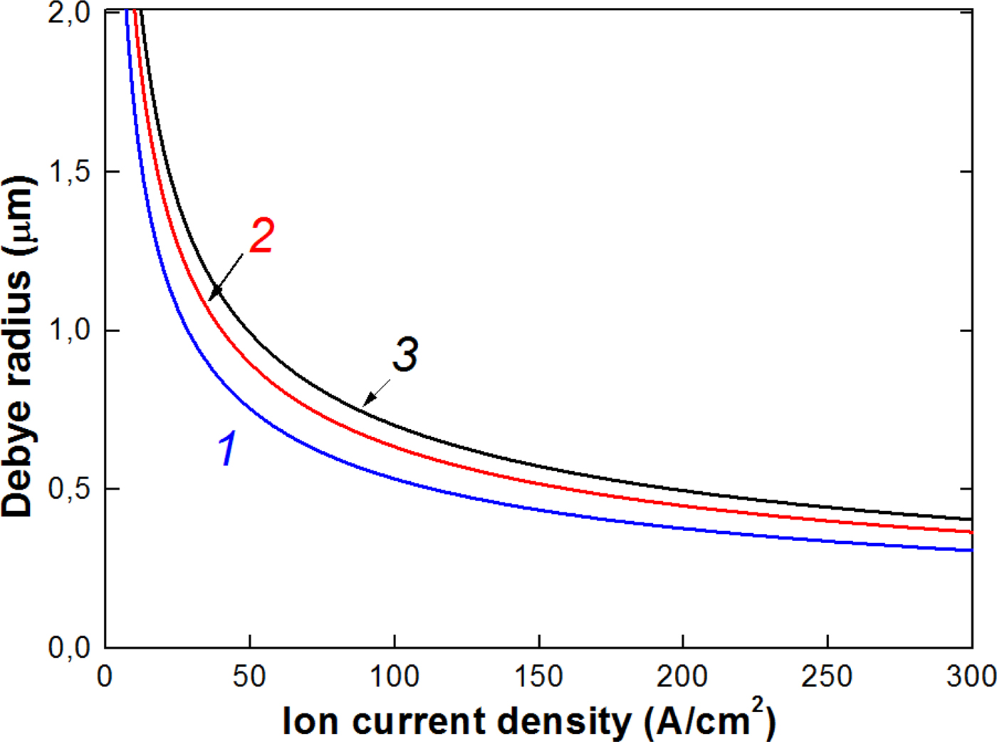
 $$\lambda _{\rm D} = 0.3\displaystyle{{U^{1/4}} \over {\sqrt j}}, \,\,{\rm \mu m,}$$
with the accelerating voltage in volts and ion current density in A/cm2.
Figure 19 shows the calculation of the Debye radius for typical HIPIB parameters.
Calculation of the Debye radius for low-energy electrons in HIPIB (T e = 300 K) at an accelerating voltage of 100 kV (1), 200 kV (2), and 300 kV (3).

When using a Faraday cup with electric bias, the HIPIB diameter should be several microns, which at a current density of 30–150 A/cm2 and a load resistance of 50 Ω provides a very weak signal. Therefore, in our experimental conditions, it is more promising to use a CFC with magnetic cut-off.
Conclusion
The developed time-of-flight diagnostics makes it possible to determine the main characteristics of HIPIBs: the composition of the beam (ion type and ionization rate), the absolute values of the ion current density, and the energy spectrum for each ion type with an accuracy of ±10%. The technique has been successfully tested on different ion accelerators, which form HIPIB of a complex composition at the energy level of 6–8 GW and the concentration of up to 2 × 1013 cm−3.
We performed a comparative analysis of two types of CFCs with magnetic cut-off and with electric bias. When using a Faraday cup with electric bias, the HIPIB diameter should be a few microns to remove electrons, which at a current density of 30–100 A/cm2 and a load resistance of 50 Ω provides a very weak signal. Therefore, it is more promising to use a CFC with magnetic cut-off of low-energy electrons.
Acknowledgments
Data analysis and interpretation of experimental results were supported by Russian Science Foundation via grant no. 17-79-10140. The authors would like to thank Dalian University of Technology, especially Professors X. P. Zhu and M. K. Lei for support in maintaining experimental set-up, and in performing some of the experiments.