

1. Introduction
Survival analysis is the study of the survival of a member and the variables that affect survival until the event of interest occurs. In our study the event of interest is death and we aim to investigate the impact of demographic factors such as age, marital status, employment status and self-reported health factors such as mobility, Activities of Daily Living (ADL) and Instrumental Activities of Daily Living (IADL) impairment and Noncommunicable Diseases (NCD) such as Cardiovascular Diseases (CVD) and lung diseases on the lives of the English population aged 50+. We consider ELSA which is a panel study of a representative cohort of individuals aged 50 or older living in private households in England and is conducted every two years since 2002. ELSA has been extensively studied by researchers in medical and social sciences. For example, Demakakos et al. (Reference Demakakos, Biddulph, Bobak and Marmot2016) study the relationship between wealth and all-cause and cause-specific mortality using Cox proportional regression analysis and find that wealth is strongly associated with CVD and other non-cancer mortality among people aged 50–64, whereas there is a weak relationship between wealth and cancer mortality. In another study, Demakakos et al. (Reference Demakakos, Biddulph, Oliveira, Tsakos and Marmot2018) investigate the relationship between self-perceptions of socio-economic status and all-cause and cause-specific mortality using Cox proportional regression hazard model and chained equations to impute missing values. Some studies use ELSA to consider the problem of disability and factors that affect disability among the elderly. For example, d'Orsi et al. (Reference d'Orsi, Xavier, Steptoe, Oliveira, Ramos, Orrell, Demakakos and Marmot2014) apply Generalized Estimating Equation (GEE) models with 2-year lagged Poisson regression to look at the impacts of socio-economic, demographic and lifestyle on IADL, its duration and speed of recovery. Potente and Monden (Reference Potente and Monden2016) use a multinomial logistic model to study the relationship between socio-economic status and disability before death in ELSA dataset. They look at the association between income, education, wealth and disability factors such as ADL, IADL and mobility impairment among deceased individuals. Steptoe and Zaninotto (Reference Steptoe and Zaninotto2020) study the relationship between socio-economic status, represented by wealth and physical capability, sight, hearing impairment, physiological function, cognitive performance, emotional well-being and social function using covariance and logistic regression analysis while controlling for age, gender, ethnicity, education and long-term health conditions. They find that lower wealth is associated with all these problems and hence will increase the rate of ageing. In both studies, among socio-economic indicators, the impact of wealth is more significant than education and income. Torres et al. (Reference Torres, Lima-Costa, Marmot and de Oliveira2016) consider the problem of wealth inequality and disability by taking into account depression and social support using multinomial logistic regressions. Guzman-Castillo et al. (Reference Guzman-Castillo, Ahmadi-Abhari, Bandosz, Capewell, Steptoe, Singh-Manoux, Kivimaki, Shipley, Brunner and O'Flaherty2017) predict the life expectancy with and without disability using Sullivan's index (Reference Sullivan1971). They use ELSA dataset and apply a discrete-time probabilistic Markov model to examine the individual and collective impacts of CVD, dementia, disability and other diseases on life expectancy. Some of the studies in social sciences consider the impact of social interaction and well-being on survival among people in old age. Davies et al. (Reference Davies, Maharani, Chandola, Todd and Pendleton2021) apply linear mixed models and Cox proportional hazard model to study the impact of social isolation and loneliness on frailty and use multiple imputations to impute missing data. [See, also Steptoe et al. (Reference Steptoe, Deaton and Stone2015); Khondoker et al. (Reference Khondoker, Rafnsson, Morris, Orrel and Steptoe2017); Rafnsson et al. (Reference Rafnsson, Orrell, d'Oris, Hogervorst and Steptoe2020) and the references therein]. There are comparative studies that combine ELSA with data from other countries. Aida et al. (Reference Aida, Cable, Zaninotto, Tsuboya, Tsakos, Matsuyama, Ito, Osaka, Kondo, Marmot and Watt2018) consider the impact of social and behavioral factors on survival among old-aged population in Japan and England. They fill in missing values using multiple imputation methods with chained equations and apply Laplace regression models to estimate the percentile of survival time and Cox proportional hazards for sensitivity analysis. Donati et al. (Reference Donati, Fongo, Cattelani and Chesani2019) use ELSA and The Irish Longitudinal Study of Ageing to predict the development of functional disability through deep and shallow artificial neural networks. They consider declining ADLs and IADLs between two consecutive waves as a measure of frailty among participants and apply Minimum Redundancy Maximum Relevance (MRMR) algorithm to select a subset of the most significant features. Kessler et al. (Reference Kessler, Thumë, Scholes, Marmot, Facchini, Nunes, Machado, Soares and Oliveira2020) focus on the comparison of risk factors such as physical inactivity, smoking, hypertension, diabetes and high BMI which are the causes of NCD among the population aged 60+ from ELSA and Bagé Cohort study of Ageing (SIGa-Bagé). They conclude that the level of these risks among the Brazilian population is higher than the English population. They ascribe their results to the quality of healthcare and economic situations in England. Stamate et al. (Reference Stamate, Musto, Ajnakina and Stahl2022) also apply machine learning algorithms to predict the development of dementia among participants. They consider patients' general health, mental health, life satisfaction, mobility, socio-economic status, etc and apply Cox proportional hazard model with Elastic Net regularization and a Random Forest algorithm where the best split is obtained by maximizing the survival difference between subsequent nodes. They removed rows with missing values at 51% or greater and apply K-nearest neighbors with K = 5 to impute the rest and use concordance measure c-statistics which is a generalization of the Receiver Operating Characteristic curve (ROC) and the area under curve (AUC) [Heagerty and Zheng (Reference Heagerty and Zheng2005)] to evaluate the performance of their models.
After reviewing the literature related to our dataset (ELSA), we look at the literature that considers time to event analysis. Cox (Reference Cox1972) introduces Cox regression models for the analysis of the effect of categorical and quantitative variables on survival in continuous time. In our case, the exact time of death and withdrawal, i.e. censored time is unknown and we only know the year of death or whether an interviewee has participated in the follow-up interview or not. Therefore, we need to carry out a discrete-time survival analysis. Thompson (Reference Thompson1977) considers the problem of ties and introduces a model based on the grouping of failure times. He applies a logistic model based on Cox's binary hazard model and uses a modified Newton–Raphson's method to estimate the likelihood equations. Friedman (Reference Friedman1982) considers a piecewise exponential model for the analysis of censored data with covariates and uses iterative numerical methods to find Maximum Likelihood (ML) estimates. Discrete-time survival analysis has been considered by Allison (Reference Allison1982) where he compares discrete-time and continuous-time survival models and shows that the likelihood function is similar to the function for binary responses in GLMs and therefore similar estimation methods can be applied. Discrete-time survival model in the context of job duration and unemployment has been considered for example, by Petersen (Reference Petersen1986), Ham and Rea (Reference Ham and Rea1987), and Singer and Willet (Reference Singer and Willet1993). Discrete-time frailty models also known as survival models with random effects can account for unobserved heterogeneity which cannot be described by existing covariates. Scheike and Jensen (Reference Scheike and Jensen1997) study the time to pregnancy and point out that random effects models can capture the heterogeneity due to biological variation. The likelihood function of random effects models involves numerical integrations and can be solved by numerical methods such as Laplace methods [Breslow and Clayton (Reference Breslow and Clayton1993)], Gauss–Hermite quadrature (GHQ), adaptive GHQ [Davidian and Giltinan (Reference Davidian and Giltinan2003); Bolker et al. (Reference Bolker, Brooks, Clark, Geange, Poulsen, Stevens and White2009)], and Markov Chain Monte Carlo methods [Fahrmeir and Knorr-Held (Reference Fahrmeir and Knorr-Held1997); Bolker et al. (Reference Bolker, Brooks, Clark, Geange, Poulsen, Stevens and White2009)]. Davidian and Giltinan (Reference Davidian and Giltinan2003) provide a review of mixed effects models and discuss different estimation methods and the supported software. Bolker et al. (Reference Bolker, Brooks, Clark, Geange, Poulsen, Stevens and White2009) consider GLMMs in the context of ecology and evolution and look at different inference methods for hypothesis testing and model selection. [See, also, Tutz and Schmid (Reference Tutz and Schmid2016) and the references therein for a detailed discussion of discrete-time survival models and their applications in R].
In our dataset, the maximum number of observations for each participant is 5 waves, i.e. 10 person-years. However, some participants may contribute to less than 5 waves due to death, permanent or temporary withdrawals. For example, some individuals may participate only in wave 1 and then re-join in wave 5 and that means we do not have any information in waves 2, 3 and 4. In these cases, we consider the withdrawal periods as missing records and apply Multivariate Imputation by Chained Equations (MICE) to impute these records. [See, for example, Lee and Carlin (Reference Lee and Carlin2010); Azur et al. (Reference Azur, Stuart, Frangakis and Leaf2011); van Buuren and Groothuis-Oudshoorn (Reference van Buuren and Groothuis-Oudshoorn2011); van Buuren (Reference van Buuren2018)].
Longitudinal study or panel study is a useful tool in order to study the developmental pattern of the same variables over a short or long period. It is often used in clinical psychology to study changes in behavior, thoughts and emotions and in economics to study consumer trends. In actuarial science, longitudinal data has been considered by Frees (Reference Frees2004), Antonio and Valdez (Reference Antonio and Valdez2012), Antonio and Zhang (Reference Antonio and Zhang2014) in the context of experience rating and credibility theory and by Renshaw and Haberman (Reference Renshaw and Haberman2000), Richayzen and Walsh (Reference Richayzen and Walsh2002), Li et al. (Reference Li, Shao and Sherris2017) and Hanewald et al. (Reference Hanewald, Li and Shao2019) in the context of mortality and disability trend.
In this study, we use ELSA dataset and perform a discrete-time survival analysis to examine the impact of demographic and self-reported health factors on the survival of the population aged 50+. We fit a random effects model to our imputed datasets. The predictability of our model will be examined in terms of time-dependent ROC and AUC. The rest of the paper is organized as follows: in Section 2 we explain ELSA dataset and the variables of our study. Section 3 discusses the models and algorithms we use to analyze our dataset. In Section 4 we discuss our results and Section 5 concludes.
2. Data and data preparation
The English Longitudinal Study of Ageing (ELSA) is a collection of economic, social, psychological, cognitive, health, biological and genetic data. The study commenced in 2002 and the sample has been followed up every 2 years. The first cohort was selected from respondents to the Health Survey for England (HSE) in 1998, 1999 and 2001 and included people born on or before February 29, 1952, i.e. aged 50 and older. The first ELSA wave was in 2002–2003. Wave 2 took place in 2004–2005, wave 3 in 2006–2007, wave 4 in 2008–2009 and wave 5 in 2010–2011. To make sure ELSA is designed to be representative of people aged 50 and over in England, in waves 3 and 4, a refreshment cohort of people just entering their 50 s was introduced. These new cohorts are called “Cohort 3” and “Cohort 4”. The cohort number was chosen to reflect the wave in which the new sample was introduced. There is no “Cohort 2” or “Cohort 5” as no new sample was issued at waves 2 and 5. In wave 2, an End of Life interview was conducted with the purpose of finding out about the health and socio-economic situations of people just before their death. End of Life interviews have been carried out at waves 2, 3, 4 and 6. [For more information on ELSA, sampling and interview process see, for example, Steptoe et al. (Reference Steptoe, Breeze, Banks and Nazroo2013); Blake et al. (Reference Blake, Bridges, Hussey and Mandalia2015)]. Table 1 shows the number of participants in each cohort and the number of deaths among “core members” reported in waves 2, 3, 4 and 6. Core members are age-eligible sample members who participated in the HSE and are interviewed in the first wave of ELSA when invited to join [Bridges et al. (Reference Bridges, Hussey and Blake2015)]. Here, we only focus on core members and do not consider their partners.
Number of core members and end of life interviews in each wave

NatCen: Technical Report (Wave 6).
1 New cohorts were only introduced in waves 3 and 4.
2 The number of end of life interviews of the core members.
3 In wave 2 one member aged below 50 has been removed.
In this study, we collected information about age, gender, marital status, employment status, self-rated physical and health conditions of core members from waves 1, 2, 3, 4 and 5 and retrieve information regarding their status from waves 2, 3, 4 and 6. The variables that we consider in our study are presented in Table 2. These variables are extracted from “core data” files that can be obtained from ELSA website after registration. The participants have been asked to fill in a questionnaire. The information provided is based on participants' self-assessment of their health conditions. Responses such as “refusal”, “don't know” and “schedule not applicable” are considered missing values. Our dependent variable is the status of the individuals that can be obtained from “eol” files for different waves and is coded 1 if death occurs and 0 otherwise. The age is a continuous variable which is limited to 90 to avoid disclosure. The age average ranges from 65.2 in wave 1 to 67.8 in wave 5. The gender is coded 1 for males and 2 for females. From wave 3, “civil partnership” has been added to the legal marital status. In our study, the marital status has two categories: “married” (being in a partnership) and “single” (no partnership including divorced and widowed). There are 8 categories of employment status. We combine “semi-retired”, “other”, “looking after home or family” and “unemployed” as “other”.
Dependent and independent variables of the study

The questions relating to health factors are different in different waves. We selected questions which are common among all waves. In wave 1 participants were asked to select the physical difficulties and diseases that they suffered, from a list and from wave 2 they were asked about the health conditions carried forward from the previous wave and the newly-diagnosed conditions. In other words, if a participant confirms a particular disease, this can be either the disease from the previous year or the newly-diagnosed disease. Therefore, for these variables, we consider “not applicable” as no experience of physical difficulty or disease. The variables mobility, ADL and IADL score are discrete. They represent the number of activities with which participants have difficulties or need help. For example, a score of “0” means that the participants have not reported difficulties in performing any activities related to mobility and a score of “10” means they have reported difficulties in performing all 10 activities. The scores for ADL and IADL are similarly defined. The remaining variables are dichotomous.
Figure 1 shows the number of times that a problem related to mobility, ADL and IADL has been reported. We observe that difficulties in performing physical activities, which are represented by green circles, are more frequent than difficulties in performing IADL, which are represented by red circles. Further, difficulty with “stooping” is the most reported problem and difficulty with “picking up a 5p coin” is the least reported problem among mobility impairment. Out of activities related to ADL, difficulty with “dressing” is the most reported problem and difficulty with “eating” is the least reported problem. The most reported problem under IADL is difficulty with “pushing or pulling large objects” and the least reported problem is difficulty with “taking medications”.
The number of times a problem has been reported.

Table 3 shows the “number of death”, “at risk”, i.e. the number of members exposed to risk and “hazard probability”, i.e. the probability of event occurrence in each interval. Figure 2 shows the baseline hazard function in our model which is the hazard function for the reference individual in the model (see Section 3).
Baseline hazard function: log (−log (1 − λ(t)) = γ 1T 1 + γ 2 T 2 + γ 3 T 3 + γ 4 T 4 + γ 5 T 5.

Number of deaths and at risk in each time interval

2.1. Missing values
Table 4 shows an example of the type of data and missing values that we are dealing with in our study in long format. In this table, we have 5 periods with repeated observations of variables such as V 1, V 2, … for individuals with ID numbers 1, 2, 3 and 4. Individual 1 participates in interviews within the periods [t 1, t 2), …, [t 4, t 5) and dies in the period [t 4, t 5). Individual 2 participates within the period [t 1, t 2) and [t 2, t 3) and withdraws in the period [t 2, t 3), i.e. right-censored. Individual 3 participates within the period [t 2, t 3) and dies in the same period. Therefore, we do not have any information about this individual for the period [t 1, t 2) except for age, gender and status assuming that in the period [t 1, t 2) the individual was 2 years younger and the gender is fixed. This individual is left-censored. Individual 4 participates within the periods [t 1, t 2) and [t 2, t 3), withdraws temporary in the period [t 3, t 4), rejoins the study in the period [t 4, t 5) and dies in that period. Therefore, the only information that we have from this individual in the period [t 3, t 4) is age, gender and status. In this study, all NAs are considered missing values.
An example of longitudinal data with missing values (long format). V 1, V 2, … are variables such as age, ADL score, etc.

We assume that missing values are independent of the occurrence of death, that is participants have not withdrawn from the study because they were more or less likely to die. Given that the interviews are conducted every two years, we expect each participant to be two years older in the follow-up interview, so the missing values of the variable age can be easily filled in. However, this means that the minimum age is now below 50 and the age is not capped at 90. The variable gender is “time-invariant” and complete. The next variable to consider is the employment status. We set all missing values as “retired” for participants aged 60 and above. To fill in the missing values of employment status and marital status we use Last Observation Carried Forward (LOCF) method. LOCF is a single imputation method in which the last observed record of an individual is used to fill in subsequent missing values. However, it is not recommended by the National Academy of Sciences for the imputation of missing values in clinical trials and/or without justificationsFootnote 1. Here we do not expect much changes in employment status and marital status among the elderly. After the implementation of LOCF, we still have two participants with missing values that we remove from our dataset. For other variables such as physical disability and diseases, we use multiple imputation methods. MICE, known as “fully conditional specification” or “sequential regression multiple imputation”, can handle different types of variables such as continuous, binary and categorical variables. In R package mice, we use the “predictive mean matching” (pmm) method for the imputation of mobility, ADL and IADL and “logistic regression” for the imputation of other variables. One of the advantages of pmm is that it always finds values that have been actually observed in the data, i.e. all imputed values are based on the possible observed values and this reduces the possibility of model misspecification and allows the algorithm to be used for any data types. The assumption underlying this method is that the distribution of the missing data is the same as the distribution of the observed data. Figure A3 in the Appendix compares the distribution of the imputed values of these 3 covariates with the distribution of the observed values. We explain pmm and logistic algorithms in Section 3.4. We create 5 complete datasets with 10 iterations. The number of iterations can be determined by inspecting the trace lines generated by the algorithm. In Figures A1 and A2 we cannot detect any trends as expected and therefore 10 iterations is reasonable [van Buuren and Groothuis-Oudshoorn (Reference van Buuren and Groothuis-Oudshoorn2011)]. MICE is computationally expensive for a large number of variables. Therefore, we consider a model with a very simple predictor matrix by setting all variables except status equal to zero [van Buuren (Reference van Buuren2018), page 300].
The 5 datasets are identical for the observed data but differ in the imputed values. We store these 5 complete datasets and perform our analysis on each dataset instead of combining the results using Rubin's rules. Table 5 shows the mean for mobility, ADL and IADL scores and the number of participants with a particular disease for 5 datasets after imputation, i.e. datasets I, II, III, IV and V.
Mean and frequency of the variables for 5 new datasets. 1: Mean.

3. Models
In this section, we look at discrete-time survival models, also known as time-to-event models. When we are working with survey data the information is not available at the exact point in time and we only know the period in which the event of interest occurs, which is usually every one year or in our case every two years. We can divide the underlying continuous-time process into intervals [0, a 1), [a 1, a 2), …, [a t−1, a t), [a t, ∞). Let T be a discrete-time random variable, where T = t means the event has happened in the interval [a t−1, a t). Censoring is common in survival analysis and right-censoring occurs when the participants are lost to follow up or when the study ends. For individual i, i = 1, …, n, let T i denote duration times and U i be right-censoring times. Let t = min (T i, U i) be the observed discrete time and δ i be the censoring indicator:

Let y it ∈ {0, 1} be the event indicator. We then have

In the following, we explain survival models and the estimation methods in GLM [McCullagh and Nelder (Reference McCullagh and Nelder1989)] and GLMM framework.
3.1. GLMs with time-varying covariates
Let xit = (x i1, …, x it)T be a vector of covariates and i = 1, 2, …, n be the sample size. For individual i, we then define the hazard function in discrete time by

which is the conditional probability that an event occurs at time t given that it has not already occurred and η it is the linear predictor, given by

In Equation (3), h(.) is a function, which is assumed to be strictly monotonically increasing with the inverse function g = h −1 which is known as the link function. Therefore, Equation (3) can also be written as

The function h(.) is selected such that the value of the discrete-time hazard is restricted to the interval [0, 1]. Common candidates are logistic, probit, Gompertz (clog-log), and Gumbel (log-log) link functions. Further, γ 0t is the intercept which may vary over time and is interpreted as a baseline hazard and γ is the vector of parameters. Thompson (Reference Thompson1977) shows that logistic and clog-log link functions give rise to similar results. In this study, we choose clog-log link function, where h(η) = 1 − exp ( − exp (η)). Hence, the hazard function is given by

which can also be written as

We can also define the discrete-time survival function by

which is the probability that death occurs after time t given the covariates. Hence the unconditional probability of death at time t, i.e. the probability that death occurs within the interval [a t−1, a t) is given by

Assuming that censoring is non-informative and does not depend on the parameters, the likelihood function for observation i is given by

Substituting (7) and (8) and taking the logarithm yields the log-likelihood function [Allison (Reference Allison1982); Singer and Willet (Reference Singer and Willet1993)]

which can be rewritten as

Equation (11) can be solved using numerical methods such as Iteratively Reweighted Least Squares (IRLS) in R. [See, McCullagh and Nelder (Reference McCullagh and Nelder1989)].
3.2. GLMMs
In this section, we explain random effects models. Let b i be a random intercept specific to individual i that follows a mixing distribution with density f(.). We define the discrete-time hazard function for individual i by

where $\eta ^{\prime}_{it}$ is the linear predictor given by

Similar to GLMs we define the survival probability in discrete-time by

Since our model only includes a random intercept, we call it the random intercept model. Estimation of parameters in GLMMs is not as straightforward as the GLMs. To estimate the parameters, we need to integrate the likelihood function over all possible values of the random effects, i.e.

To handle the integral, we need to use numerical integration methods. In this study, we use Gauss–Hermite quadrature which is a numerical method used by “glmer” in R package “lme4” to approximate the value of integrals of the following kind

The idea is that we can approximate an integral as a sum of polynomials, i.e.

where w i and x i are the weights and quadrature points, respectively. Parameters are chosen so that this approximation is exact for polynomials f(x) up to and including degree 2n − 1, where n is the number of points in the summation. Suppose n = 3, then we have 3 unknown w, 3 unknown x and polynomials with degrees up to and including 5, i.e. f(x) = 1, f(x) = x, …, f(x) = x 5. Therefore, we have 6 equations to find 6 unknowns. The values of w i and x i for different n can be obtained from Table 25.10 in Abramowitz and Stegun (Reference Abramowitz and Stegun1964).
3.3. Optimization
Parameter estimation in the above models is an optimization problem as we either need to maximize the likelihood function or minimize the negative likelihood function, i.e. min f(x), x ∈ R n. The common approach to solving such problems is to take a derivate of the objective function (here, the likelihood function). However, when the objective function is not smooth and/or is complicated, we can use gradient-free optimizers and numerical methods to find the optimum value. In Table A2 in the Appendix, we provide a comparison of some of the gradient-free algorithms in terms of the estimated parameters, convergence and the time taken until convergence. In the following, we briefly explain the optimizers in this table.
Nelder-Mead simplex algorithm
This is a direct search method, which means that it calculates the value of a function and compares it to its values at other points. It uses a simplex which is a shape consisting of n + 1 vertices in n dimensions, such as a triangle in 2 dimensions. To optimize a function in 2 dimensions, we need three arbitrary points and find the value of our function at those points, say, f(a) < f(b) < f(c) in this step a is the best point as our function takes the minimum value at a and c is the worst point. Then we reflect c through the centroid of a and b. If the new point is better than b, we replace the old c with our new c. If the new c is better than a, then we extend c even further. The algorithm takes different steps such as reflection, extension and contraction until it converges and the optimum point is obtained (Nelder and Mead (Reference Nelder and Mead1965).
Bound Optimization BY Quadratic Approximation (BOBYQA)
This is a trust region method, where a surrogate model is used. If f is a complicated function, we can use a simpler function like $\tilde{f}$ for optimization that approximates f well in the trust region. The common candidate for $\tilde {f}$
 is a quadratic function obtained by Taylor series, i.e.

where x k is the point at the kth iteration, $\nabla f$ is the gradient and H is the Hessian. This algorithm, does not require the exact calculation of the gradient and Hessian matrix, instead it uses interpolation equation $\hskip2.2pt\tilde {\hskip-2.2ptf}_k( x_i) = f( x_i)$
 for i = 1, 2, …, m to estimate the gradient and the Hessian matrix, where m is chosen from the interval [n + 2, (n + 1)(n + 2)/2]. We then minimize $\hskip2.2pt\tilde {\hskip-2.2ptf}$
 subject to a trust region with radius δ at each iteration

To determine the size of the δ at each iteration we define the ratio

where x* is the solution to the subproblem in each iteration. If r is greater than a threshold, say, 1 then, the trust region is increased, i.e. δ increases as the algorithm is moving in the right direction towards the optimum point, otherwise, the trust region is decreased. The algorithm terminates when the radius of the trust region is less than a given tolerance level [Powell (Reference Powell2009); Rios and Sahinidis (Reference Rios and Sahinidis2013)].
L-BFGS-B
This method is based on quasi-Newton optimization method. The idea is that as we can use Newton's method to find the roots of a function, we can also apply this method in order to find the roots of the gradient of a function, i.e.

Since H −1 does not always exist and it is computationally expensive, it can be replaced by another function which is an approximation to H. Therefore, Equation (15) in quasi-Newton algorithms can be written as

where B is an approximation to H. The algorithm starts with an arbitrary B, say, I an identity matrix and updates B until convergence. The difference between different classes of quasi-Newton methods such as Broyden-Fletcher-Goldfarb-Shanno (BFGS) and limited memory BFGS (L-BFGS-B) is on how B is determined. For example, L-BFGS-B is more suitable for large scale optimization problems with restricted memory [Liu and Nocedal (Reference Liu and Nocedal1989); Nash and Varadhan (Reference Nash and Varadhan2011)].
Other algorithms in Table A2 include nonlinear minimization with box constraints (nlminb) which is based on Newton optimization methods subject to a box constraint, alternative versions of Nelder-Mead and bobyqa which are provided via “nloptr” wrapper package.
3.4. Imputation algorithms
Let Y be a variable that contains the missing values. We denote the observed values by y obs and the missing values by y mis. Let also Xobs be a matrix of covariates for which y is observed and Xmis be a matrix of covariates for which y is missed. In this study, we use predictive mean matching and logistic regression to impute missing values.
Predictive mean matching
This method is based on Bayesian regression and we need to draw samples from the posterior distribution of the parameters. This is an important step in MICE algorithm to ensure uncertainty in the imputations [van Buuren (Reference van Buuren2018)].
Step 1 Let yobs ~ N(Xobsβ, σ 2I), where X is a matrix with n rows and k columns which represent the number of covariates. Here we assume β and σ 2 are both unknown. Suppose the prior distribution of β|σ 2 is given by
(17)$$\beta \vert \sigma^2 \sim N_k( 0,\; \sigma^2 {\bf V}_0) $$and the prior distribution of σ 2 by (18)$$\sigma^2 \sim {\rm Inv-Gamma}\left(a_0 = {\nu_0\over 2},\; b_0 = {1\over 2}\nu_0 s^2_0\right) = {\rm Scale-inv-}\chi^2( \nu_0,\; s^2_0) = \nu_0 s^2_0 \chi^{-2}_{\nu_0}.$$Then, the posterior distribution has the following form [see, for example, Box and Tiao (Reference Box and Tiao1973); Murphy (Reference Murphy2012)]$$\eqalign{\,p( \beta,\; \sigma^2 \vert {\bf X}_{obs},\; {\bf y}_{obs}) & \propto p( \beta \vert {\bf X}_{obs},\; {\bf y}_{obs},\; \sigma^2) p( \sigma^2 \vert {\bf X}_{obs},\; {\bf y}_{obs}) \cr & \propto N( \beta \vert \beta_n,\; \sigma^2 {\bf V}_n) {\rm Inv-Gamma}( a_n,\; b_n) ,\; }$$where
• $\beta _n = {\bf V}_n {\bf X}^{T}_{obs} {\bf y}_{obs}$
• ${\bf V}_n = ( {\bf X}^T_{obs} {\bf X}_{obs} + {\bf V}^{-1}_0) ^{-1}$
• a n = a 0 + n/2
• $b_n = b_0 + ( {\bf y}^T_{obs} {\bf y}_{obs} - \beta _n^{T} {\bf V}_n^{-1} \beta _n) /2$
.
Here, we only need the first two expressions. (See, Appendix A.2 for details).
Step 2 Let [Box and Tiao (Reference Box and Tiao1973)]
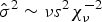
$$s^2 = ( {\bf y}_{obs} - \hat{{\bf y}}) ^{T} ( {\bf y}_{obs} - \hat{{\bf y}}) / \nu ,\; $$where $\hat {{\bf y}} = {\bf X}_{obs} \hat {\beta }$ is the vector of predicted values of y. Then from (18) we have $\hat {\sigma }^2 \sim \nu s^2 \chi ^{-2}_{\nu }$. Draw a random variable $g \sim \chi ^{2}_{\nu }$ with ν = n − k, where n is the number of rows with observed values and k is the number of covariates for which y is observed. Calculate $\hat {\sigma }^2 = s^2 / g$.Step 3 Draw k random values Z ~ N(0, 1).
Step 4 Calculate $\beta ^{\ast } = \hat {\beta } + \hat {\sigma } {\bf z}_1 {\bf V}^{1/2}$
.Step 5 Calculate y* = Xmisβ*.
Step 6 For each missing value of y*, find the closest predicted values, i.e. $\hat {y}$
.Step 7 Choose d values of $\hat {y}$
which are close to y* and randomly choose one of them. The values of d depend on the sample size. Small d may lead to repetition and large d may increase bias [van Buuren (Reference van Buuren2018)].Step 8 Find the corresponding observed value of $\hat {y}$
and set y mis = y obs.Example: Suppose ADL score for individual I is NA and the observed values of ADL, y, for individuals II, III, IV and V are 5, 6, 3 and 4, respectively. Using $\hat {\beta }$
we can estimate ADL, $\hat {y}$, for these individuals, say, 7, 5, 4 and 3, respectively. Then suppose using β*, we find y* = 6. The 3 closest $\hat {y}$ to 6 are 7, 5 and 4 with the corresponding observed values of y = 5, 6 and 3. The algorithm then selects one value from the observed values of y randomly to impute the missing ADL for individual I.












Inverting the matrix in Step 1 may not be numerically stable. MICE applies Cholesky decomposition for matrix inversion [Murphy (Reference Murphy2012); van Buuren (Reference van Buuren2018)].
Logistic regression
In this section, we explain imputation using logistic regression method.
Step 1 Consider the binary model:
$$p( y_{obs} = 1 \vert {\bf X}_{obs},\; \beta) = {1\over 1 + \exp( \hskip-2pt-\!\beta^{T} {\bf X}_{obs}) }.$$MICE uses Iterative Reweighted Least Squares (IRLS) to estimate β. Therefore, the negative log-likelihood function is given by(19)$$NLL\, \colon = l = - \sum_{i = 1}^n \left[y_{i, obs} \log p( x_{i, obs};\; \beta) + ( 1-y_{i, obs}) \log( 1 - p( x_{i, obs};\; \beta) ) \right].$$Taking the partial derivative with respect to β yields(20)$${\bf g} = {\partial l\over \partial \beta} = \sum_{i = 1}^n [ p( x_{i, obs};\; \beta) - y_{i, obs}] {\bf x}_{i, obs} = {\bf X}_{obs}^T ( {\bf p} - {\bf y}_{obs}) ,\; $$and the second partial derivate gives(21)$${\bf H} = {\partial^2 l\over \partial \beta \partial \beta^T} = \sum_{i = 1}^n p( x_{i, obs};\; \beta) [ 1 - p( x_{i, obs};\; \beta) ] {\bf x}_{i, obs} {\bf x}_{i, obs}^T = {\bf X}_{obs}^T {\bf W} {\bf X}_{obs},\; $$where ${\bf W} = {\rm diag}( p( x_{i, obs};\; \beta ) [ 1-p( x_{i, obs};\; \beta ) ] )$. Beginning with Newton–Raphson algorithm we have$$\beta_{new} = \beta_{old} - {\bf H}^{-1} {\bf g}. $$Substituting (20) and (21) yields(22)$$\beta_{new} = ( {\bf X}_{obs}^T {\bf W} {\bf X}_{obs}) ^{-1} {\bf X}_{obs}^T {\bf W} {\bf z},\; $$where z = Xβold + W−1 (y − p) (see Appendix A.3 for details.). Since each iteration solves the weighted least squares problem, i.e. (z − Xβ)TW (z − Xβ), this method is known as IRLS. [See, for example, Hastie et al. (Reference Hastie, Tibshirani and Friedman2009); Murphy (Reference Murphy2012)]Step 2 Calculate the estimated covariance matrix of $\hat {\beta }$
, i.e. V = H−1 = (XTWX)−1 where W is as defined in (21). Murphy (Reference Murphy2012)Step 3 Draw k random values Z ~ N(0, 1).
Step 4 Calculate $\beta ^{\ast } = \hat {\beta } + {\bf z}_1 {\bf V}^{1/2}$
.Step 5 Calculate the predicted probability based on missing values, i.e. p* = 1/[1 + exp (−Xmisβ*)].
Step 6 Draw random variates from the uniform distribution U(0, 1).
Step 7 Set imputations y mis = 1 if u ≤ p*, and y mis = 0 otherwise.






4. Results
In this section, we discuss the models that we fit to our datasets I, II, III, IV and V. In each dataset, we have 59, 265 observations and 14, 964 unique individuals. We then divide our datasets into 70% training set and 30% validation set (test set). We will use the test set in Section 4.1 to compare the predictive power of our fitted models. In our training set, we have 41, 543 observations and 10, 475 unique individuals. In order to select our variables, we first build a “full model” by incorporating all variables and fitting a GLM with a clog-log link function. The results based on training set I are provided in Table 6. The variables “time”, “gender”, “age”, “employment status”, “IADL”, “heart attack”, “diabetes”, “lung disease” and “cancer” are statistically significant at $0.1\%$ and marked with three asterisks, which indicate that these variables have a significant impact on the hazard probability of death. We then use these significant variables from the “full model” and build our reduced GLM. We can see a similar pattern in the “reduced model” with greater log-likelihood at the expense of losing 10 variables. We test the null hypothesis that all these variables are identical. The difference between deviances of the full model and the reduced model is 9.4 which is less than 5% critical value of a χ 2 distribution with 10 degrees of freedom and therefore we do not have sufficient evidence against our null hypothesis. We consider the variables of our reduced model and fit a random effects model (GLMM) to our training set I. As we discussed in Section 3.2 fitting GLMMs involve numerical optimization which is computationally expensive with the possibility of convergence issues. We apply the adaptive Gauss–Hermite quadrature [Kabaila and Ranathunga (Reference Kabaila and Ranathunga2019)] with 9 quadrature points, i.e. nAGQ = 9. The higher the quadrature points, the more exact the approximation is. However, this happens at the cost of speed. Also, according to Tutz and Schmid (Reference Tutz and Schmid2016) for simple models with random intercept, 8 to 15 quadrature points yield stable estimates. Since most of our variables are binary and the scale of age is different from other variables, we have convergence issues which can be resolved by scaling the variable age. This can be done by subtracting the column mean and dividing by the standard deviation. After that, we try several optimizers (see Table A2 in Appendix). As we can see, even after scaling age, we have convergence warnings for most of the optimizers. Bates et al. (Reference Bates, Mächler, Bolker and Walker2015) recommend “bobyqa”. We use this optimizer with the maximum number of function evaluations before termination of 100, 000. As we can see both Akaike Information Criterion (AIC) and Bayesian Information Criterion (BIC) have reduced. The random effect shows the individual-level effects, i.e. how much does an individual differ from the population? This variability is given by a variance of 1.346. The results of GLMM fitted to datasets II, III, IV and V are provided in Table A1 in Appendix. As we can see the estimated parameters and the information criteria for these datasets are reasonably close.
Coefficient and standard error estimates of models

+p < 0.1, *p < 0.05, **p < 0.01, ***p < 0.001.
1 Scaled.
To interpret the coefficients in a regression model with a clog-log link function, we note that −log (1 − x) ≈ x. Therefore, from Equation (6), λ(t|x) ≈ e η, where η is the linear predictor. Negative coefficients correspond to a negative effect on the hazard probability and positive coefficients correspond to a positive effect on the hazard probability. The variable “time” has a negative coefficient which means that as time passes we expect improvement in hazard probability, i.e. mortality. The coefficient of gender is negative which means that the probability of mortality for females is less than the probability of mortality for males. The coefficient of age is positive, which means that death is more likely as people get older.
Mortality trends
Figure 3 shows the probability of hazard for males (solid lines) and females (dashed lines) who are healthy, retired and in partnership. This figure is based on GLMM and each curve represents the probability of death for the average population at a particular age during 5 waves. We can observe that the probability of death decreases over these 5 waves, which suggests an improvement in mortality. From wave 1 to wave 2 which corresponds to the years 2002–2003, the curves are relatively flat. From wave 2 to 4, we can see a steeper downward slope. This period corresponds to the years 2003–2009. The steepest slope is in wave 5 which is during 2010–2011. This suggests a greater mortality improvement during these years. We can also observe that this improvement is more pronounced among males than females. The mortality improvement happens faster in older ages. This mortality trend is in agreement with Deaths Registered in England and Wales: 2013, Figure 1Footnote 2. We can see similar trends in terms of survival probability in Figures 4, 5 and 6. In these figures, which are also based on GLMM and average population, the green curve represents the survival probability for a healthy individual. Comparing the green curve of the plots in Figure 4, we can see a sharper negative slope in survival probability among males (left plot) than among females (right plot) before wave 4. After wave 4, the slope is less steep on the left plot than on the right plot compared with before wave 4. In other words, between waves 4 and 5, the improvement in mortality among males is more than the improvement in mortality among females.
Hazard probability for males (solid lines) and females (dashed lines), retired, in relationship, with no disease (population).

Adjusted survival probability for different ADL scores (solid line) and IADL scores (dashed line) for a male (left) and female (right) aged 65 in wave 1, retired, in relationship, with no disease (population).

Adjusted survival probability for different diseases for a male (left) and female (right) aged 65 in wave 1, retired, in relationship (population).

Adjusted survival probability for different IADL scores for a male, aged 65 in wave 1, retired, in relationship, individual (solid line) and average population (dashed line).

Socio-economic factors
Now, we consider the coefficient of “employment”, where the reference category is “employed”. Employment 3, 4 and 5 correspond to “permanently sick or disabled”, “retired” and “self-employed”, respectively. The positive coefficients, although not always statistically significant, suggest an increase in the risk of death for a retired, disabled and self-employed compared with an employed individual. Similar results have been found by Sorlie and Rogot (Reference Sorlie and Rogot1990) for the US population. They find that the mortality rate is particularly higher for those who are unable to work. In our study, we can see that the coefficient of employment 3 (permanently sick or disabled) is higher than the coefficient of other categories. In another study, Morris et al. (Reference Morris, Cook and Shaper1994) find that the risk of death for British men who are unemployed is much higher than for those who are employed. They even report a higher risk of mortality among people who retired early for reasons other than illness. The results for the relationship between mortality and self-employment are mixed. Our result shows that self-employed people have a higher probability of death. Toivanen et al. (Reference Toivanen, Griep, Mellner, Vinberg and Eloranta2016) find that mortality from CVDs and suicide is lower among self-employed in Sweden, whereas Gauffin and Dunlavy (Reference Gauffin and Dunlavy2021) find that poor health conditions are more common among self-employed than employed people in Sweden. Gonçalves and Martins (Reference Gonçalves and Martins2018) report a low mortality rate among self-employed in Portugal. We categorize “marital status” into two groups: singles which include divorced, widowed and not married categories and couples which include any form of partnership. The coefficient of marital status is negative, i.e. the risk of death for a single individual is less than the risk of death for a couple. Ebrahim et al. (Reference Ebrahim, Wannamethee, McCallum, Walker and Shaper1995) look at the relationship between marital status and mortality among British men and find that although the risk of mortality is higher among single men, divorced men are not at increased risk of mortality. Johnson et al. (Reference Johnson, Backlund, Sorlie and Loveless2000) show that the risk of mortality among single people aged 45 − 64 is higher than older American people. Rendall et al. (Reference Rendall, Weden, Faveault and Waldron2011) find that the survival probability among US married men is higher than the survival probability among married women, but they did not find mortality differences among never-married, divorced and widowed categories. In another study, Lindström and Rosvall (Reference Lindström and Rosvall2019) also point to mortality differences among married men and women. They show that the risk of mortality is higher among unmarried, divorced and widowed men, but there are no significant differences in mortality among women with different marital status in Sweden. Ramezankhani et al. (Reference Ramezankhani, Azizi and Hadaegh2019) study all-cause and cause-specific mortality for different marital status among Iranian population and find that marital benefit is different among men and women. Their results show that the risk of mortality among never-married men is higher than among never-married women.
Disability factors
We then consider the coefficients of factors related to disability: mobility, ADLs and IADLs. All these disability factors are significant and have a positive impact on mortality. This is in agreement with other studies that see disability factors as predictors of mortality. For example, Scott et al. (Reference Scott, Macera, Cornman and Sharpe1997) show that there is a direct relationship between mortality and disability factors among American population. Gobbens and van der Ploeng (Reference Gobbens and van der Ploeng2020) find similar results among Dutch population and Yang et al. (Reference Yang, Du, Liu, Lao, Sun and Tang2021) among Chinese population. In Figure 4 we compare survival probability for different levels of ADLs and IADLs between females and males by controlling age, marital and employment status factors. We can observe that the slope of survival curves is steeper for males (left plot) than for females (right plot), which indicates survival differences due to disability factors between males and females. This is in agreement with Pongiglione et al. (Reference Pongiglione, De Stavola, Kuper and Ploubidis2016) where they find a strong relationship between mortality and disability factors in ELSA participants and survival inequality among men and women. However, their findings are based on binary classifications of disability and they do not consider different levels of severity of disability. In another study, they point out that ordinal classifications of disability are more informative than binary classifications of disability [Pongiglione et al. (Reference Pongiglione, Ploubidis and De Stavola2017a)]. In Figure 4 we can also observe that IADLs contribute more to a decrease in survival probability than ADLs. Further, as IADL score increases, the survival probability falls faster. However, we can see that slope of the curves is less steep in the last wave which indicates an improvement in mortality due to disability during that period. Pongiglione et al. (Reference Pongiglione, Ploubidis and Stavola2017b) also look at disability trends between 2002–2012 by classifying disability into no disability, mild, moderate and severe groups and conclude that severe and moderate disability has improved among women, but moderate disability has increased and severe disability has been stable among men.
Disease trends
We expect all diseases to have a positive impact on the risk of death. However, in our full model, the coefficients of “angina” and “asthma” are negative, although not statistically significant and therefore they are not included in the reduced model and GLMM. The coefficient of “arthritis” is negative and significant at 5% which does not meet our expectations. However, this does not necessarily mean that arthritis has a negative effect on mortality. Table 7, shows the observed number and proportion of deaths and survivors for different diseases. For example, there are 288 cases that arthritis has been observed together with death and 14, 025 cases that arthritis has been reported without the occurrence of death. The proportion of reported arthritis without the occurrence of death is about $34\%$ which is considerably higher than other diseases. Mendy et al. (Reference Mendy, Park and Vieira2018) show that there is no relationship between self-reported arthritis and the risk of death. However, they find that knee arthritis is associated with a higher risk of CVDs and diabetes and therefore death. Similar results have been found by Turkiewicz et al. (Reference Turkiewicz, Kiadaliri and Englund2019) that arthritis does not lead to increased mortality, but knee and hip arthritis are associated with a higher risk of CVDs as a result of the inability to walk and/or be active. Figure 5 shows the adjusted survival probability for a male (left plot) and female (right plot) who is retired, in partnership, aged 65 in wave 1 and only suffers from one disease. The green curves show the survival probability for a healthy individual and the brown one shows the survival probability for an individual who only suffers from cancer. We can observe that the survival probability for some diseases is very close. In that case, one of the causes of death is shown by a dashed line. According to this figure, cancer contributes to a decrease in survival probability much more than other diseases. The second largest contribution to death is heart failure and the third one is Alzheimer's. This pattern is in line with UK government statistics for the leading causes of death amongst people aged 75 in 2007Footnote 3, where the largest proportion of death was reported to be due to cancer, chronic heart disease and dementia. In our full GLM, although the coefficient of dementia was positive, it was not statistically significant and therefore dementia was removed in our reduced GLM and GLMM. However, as we can see it is one of the causes of death that contributes to mortality among the old population even more than stroke, heart attack, lung disease and diabetes. In this figure, we can also observe that the survival probability for an individual with diabetes, illustrated by blue solid lines, and the survival probability for an individual who had a stroke attack, illustrated by pink dashed lines, is almost the same. In fact, the probability of death among diabetics is about $49.7\%$
 higher than healthy people and the probability of death among those who had a stroke attack is about $46\%$
 higher than those who did not have a stroke attack. Perhaps the reason that the probability of death for these two causes is so close is that according to research diabetics are exposed to a higher risk of death due to stroke. [See, for example, Hewitt et al. (Reference Hewitt, Guerra, del Carmen Fernändez-Moreno and Sierra2012); Lau et al. (Reference Lau, Lew, Borschmann, Thijs and Ekinci2019), and the references therein]. Similarly, we can observe that the survival probability for an individual with lung disease, illustrated by magenta solid lines, is very close to the survival probability for an individual who had a heart attack, illustrated by dark blue dashed lines. In fact, controlling for other factors, the hazard ratio for an individual with lung disease is 1.98 and for an individual with a heart attack is 2. Research shows that there is a relationship between lung diseases and CVDs and lung diseases can lead to a higher risk of mortality due to CVDs. [See, for example, Sin and Man (Reference Sin and Man2005); Carter et al. (Reference Carter, Lagan, Fortune, Bhatt, Vestbo, Niven, Chaudhuri, Schelbert, Potluri and Miller2019)]. Further, we can observe an improvement in mortality due to different causes of death in the last wave. This figure shows that cancer, followed by heart failure, is the leading cause of death which is in agreement with Deaths Registered in England and Wales: 2012 (see, Section 1)Footnote 4. The difference in survival probability among males and females can also be detected by looking at the slope of the curves.
The reported number and proportion of deaths for different diseases in training set. Disease (1), no diseases (0)

Population and individual effects
One of the advantages of GLMM is the ability of the model to consider observations belonging to nested or hierarchical subgroups within the population. In our study, the subgroups are individuals with unique id numbers who are repeatedly surveyed over the period 2002–2012. Therefore, when we investigate the impact of one factor on the survival probability of the population, we can also look at the variability of the impact of that factor for a unique individual over the same period. In other words, we consider the effects of factors both on population and individual levels. In this study, the repeated measures are therefore treated as random effects as there are some underlying factors which are unique to each individual that have not been considered by the model. Figure 6 compares the survival probability of a unique individual (solid lines) with a unique id number for different levels of disability due to IADL difficulties with an average population (dashed lines). In this figure, we controlled age, sex, employment and marital status. We can observe that the adjusted survival probability of this particular individual in healthy status is less than the adjusted survival probability of a healthy individual on average. The reason is that this particular individual may be subject to other factors such as financial problems or family health history which have not been considered by this model. On the other hand, we can see that all solid lines for different IADL scores are above the dashed lines, which indicates that the adjusted survival probability for this individual with different levels of disability is slightly higher than the adjusted survival probability for the average population with the same level of disability.
4.1. Discrimination measures
In this section, we look at the prediction accuracy of our 3 models: GLM, reduced GLM and GLMM based on the test set. For this, we use time-dependent ROC curves which are more suitable for follow-up studies than standard ROC curves. First, we explain standard ROC curves and then the time-dependent ROC curves.
Standard ROC curve
In classification problems, where we assign our observations to different classes such as death y = 1 and survival y = 0, we consider two types of error:
• False positive (Type I error): we predict that an individual will experience an event, say, death, but they did not. In other words, we estimate $\hat {y} = 1$
, but the truth is y = 0.• False negative (Type II error): we predict that an individual will be event-free and will survive, but they died. In other words, we estimate $\hat {y} = 0$
, but the truth is y = 1.


We can illustrate these two types of error in a matrix which is known as the confusion matrix [see, Table 8]:
Confusion matrix

The in-diagonal values are related to predictions that are correct and the off-diagonal values are related to incorrect predictions. Using the information from a confusion matrix, we can define the following measures:
∙ True positive rate: Tpr (sensitivity) = TP/(TP + FN)
∙ False positive rate: Fpr (type I error) = FP/(FP + TN)
∙ False negative rate: Fnr (type II error) = FN/(FN + TP)
∙ True negative rate: Tnr (specificity) = TN/(TN + FP)
The ROC curve plots Tpr against Fpr [Murphy (Reference Murphy2012)]. The more this curve is away from the 45° line, the better is our model at discriminating the positive (y = 1) and negative (y = 0) events. Another way to measure the predictability of the model is by looking at the area under the ROC curve, i.e. AUC. The larger AUC, the better the models at distinguishing between death and survival.
Time-dependent ROC curve
Let T i be the time of death and η be the linear predictor, which represents risk score and is defined in Equations (4) and (13) for GLM and GLMM, respectively. Further, let y be the death status as defined by (2). The idea is that at each time t, each individual is classified as a case, i.e. the individual dies or control, i.e. the individual survives and we would like to see what percentage of cases and controls can be discriminated by our models for different values of thresholds c. In this case, each individual who had the role of control at the earlier time, may contribute as a case at a later time [see, for example, Tutz and Schmid (Reference Tutz and Schmid2016); Kamarudin et al. (Reference Kamarudin, Cox and Kolamunnage-Dona2017)]. To plot the ROC curve, we need sensitivity and specificity rates. The time-dependent sensitivity is defined as

which is the probability that an individual who has died (T = t) is predicted to have the hazard probability η of greater than c, indicating that cases are correctly identified (TP). The time-dependent specificity is also defined by

which is the probability that an individual who has survived (T > t) is predicted to have the hazard probability η of less than or equal to c, indicating that controls are correctly identified (TN). These probabilities change as the value of threshold c changes. In a follow-up study, the status of the individuals changes over time and some observations may be censored before time t. Therefore to calculate sensitivity and specificity we need to apply the inverse probability of censoring weight (IPCW) in order to maintain consistency and to avoid bias. Let G(.) be the survival function of the censoring times U as defined in Section 3. Then we define

If G is large, then we can conclude that with high probability censoring occurs after time t, whereas if G is small, then censoring occurs before time t and hence the number of observations fully observed up to time t is only a small part of the whole sample. To allow for this under-represented group, we use the inverse probability of censoring as the weight [Tutz and Schmid (Reference Tutz and Schmid2016)]. Therefore, sensitivity is given by

where δ is defined in Equation (1), I is the indicator function and G can be obtained from the training data similar to S(t). The only difference is that this time, the event of interest is the censoring time rather than the time of death. Further, specificity is given by

We can plot the ROC curve for different points in time and compare the predictability of the models at different times. Similarly, we can define the time-dependent AUC by

where η i, η j, T i and T j are the predictors and survival times of independent observations i and j [Tutz and Schmid (Reference Tutz and Schmid2016)]. We can use package “discSurv” in R to plot Figures 7, 8 and 9 which show the ROC curves for GLM, reduced GLM and GLMM, respectively. From these figures, we can observe that at t = 1, 2 and 3, the predictive power of GLM is better than the other 2 models and at t = 4, the reduced model performs as good as the GLM. Further, we can see that the GLMM has the worst predictive power. In fact, we know that we can use GLMM to predict the survival probability of the existing individuals, but we cannot use this to estimate the survival probability of a new individual and in the case of a new individual, it only gives the estimated survival probability of the average population. In other words, for a new individual, it only takes into account population level and not individual levels. Figure 10 compares the AUC for all 3 models at t = 1, 2, 3 and 4. We can observe that at t = 1, 2 and 3, the AUC is only slightly above 0.5. However, as t increases, the predictive power of all models represented by AUC improves. From these figures, we can conclude that GLM and reduced GLM can discriminate death and survival better than GLMM and are better at generalization than GLMM.
ROC curve for GLM based on dataset I: AUC(t = 1)=0.572, AUC(t = 2) = 0.574, AUC(t = 3) = 0.574, AUC(t = 4) = 0.614.

ROC curve for reduced GLM based on dataset I: AUC(t=1)=0.569, AUC(t = 2) =0.571, AUC(t = 3) = 0.573, AUC(t = 4) = 0.614.

ROC curve for random effects model for the population average based on dataset I: AUC(t = 1) = 0.534, AUC(t = 2) = 0.554, AUC(t = 3) = 0.562, AUC(t = 4) = 0.605.

AUC for GLM, reduced GLM and GLMM at t = 1, 2, 3 and 4.

5. Conclusion
In this study, we applied survival analysis to the English Longitudinal Study of Ageing (ELSA). We looked at the impact of demographic and self-reported health conditions on the survival of the participants. We found that the survival probability for individuals who have difficulty in performing IADLs is less than the survival probability for individuals who have difficulty in performing ADLs. We also found that the survival probability for individuals with Alzheimer's disease is less than the survival probability for individuals with diabetes. Further, cancer was the deadliest of the disease that we considered in this study. We showed that a random effects model can distinguish between individual-level and population-level hazard probability. One of the problems with survey data is missing values and, in particular, temporary withdrawals of the participants. To address this issue we applied Last Observation Carried Forward (LOCF) method, which is a single imputation method, to fill in the missing values related to “employment status” and “marital status”. For the rest of our covariates, we used MICE, which is a multiple imputation method. We produced 5 datasets and applied our analysis to each dataset. We found that the results under all these 5 datasets are very close and therefore, we performed our analysis based on only one dataset. The results of this study about the survival probability and factors that affect the survival probability can be used in areas such as life insurance and health insurance.
Acknowledgements
I wish to thank the referees and the editors for valuable comments and suggestions that led to a substantial improvement of this article.
Appendix A: Appendix
A.1.
A.2. Posterior distribution of β and σ 2
Let Y ~ N(Xβ, σ 2 I); β|σ 2 ~ N k(0, σ 2 V 0) and σ 2 ~ Inv-Gamma$( a_0 = \nu _0/2,\; b_0 = \nu _0 s^2_0/2)$ . To find the posterior distribution of β and σ 2 we have

The first term is the likelihood function which is given by

First we consider the exponential term:

where $\hat {\beta } = ( X^T X) ^{-1} X^T y$ . The last term is equal to 0 since

Coefficient and standard error estimates of a random effects model based on datasets II, III, IV and V

Trace lines do not show any trends after 10 iterations.

Trace lines do not show any trends after 10 iterations.

Comparison of the distribution of the generated dataset (red curve) with the distribution of the observed dataset (blue curve).

Comparison of different optimizers

Substituting for $\hat {\beta }$ in the first term, we have

which is equal to 0 since [(X T X)−1]T X T X = [(X T X)T]−1 X T X = (X T X)−1 X T X = I. Then we consider the second term in Equation (A1) which is the prior density of β|σ 2 and is given by

and the third term in Equation (A1) is the prior density of σ 2 which is given by

Combining (A2), (A4) and (A5), posterior distribution is proportional to

Next, we consider the first two exponential terms. Using the result in (A3), we have

where in the last term we use the fact that

Our aim is to write (A7) in a quadratic form. Consider

Comparing the above expression with (A7), $\beta _n = \mu = S^{-1} ( X^T X \hat {\beta })$ and $V_n^{-1} = S = X^T X + V_0^{-1}$
 . Therefore, we can write (A7) as

Substituting in (A6), we have

which is the posterior distribution of (β, σ 2).
A.3. Gradient and Hessian matrix for a logistic regression
Consider x i = (x i1, …, x id)T. In Equation (20), we first consider the first logarithm

Taking the partial derivative with respect to β j gives

Then we take the second logarithm

Taking the partial derivative with respect to β j gives

Hence the gradient is given by

where X is a design matrix and is given by

Next we look at the Hessian matrix by taking the second partial derivative of l

where W is a diagonal matrix given by

We can now show that the application of Newton–Raphson method results in an equation which is the solution to a weighted least square problem.

which is the solution to the following problem



