1. Introduction
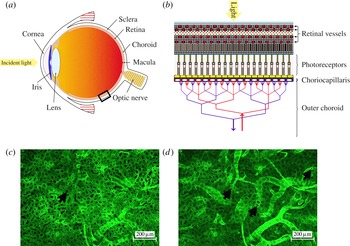
The conversion of photons into electro-chemical impulses transmitted to the brain is achieved by the eye through a set of elements organised with remarkable complexity. The cornea, the iris and the lens, located anteriorly, direct and scatter light towards the back of the eye (see figure 1
a). The retina, which contains the photoreceptors responsible for the conversion of light into electric impulses, the choroid, which is a highly vascularised layer of tissue, and the sclera are the three juxtaposing layers composing the back of the eye. The retina is supplied with metabolites by a dual circulatory system. The inner two-thirds of the tissue are nourished by the retinal vasculature. The outer third part of the tissue, which contains the photoreceptors, is solely supplied by the choroid. Most of the exchanges between the outer retina and the choroid occur at a
 $10{-}20~{\rm\mu}\text{m}$
thick layered network of capillaries located underneath the retina and called the choriocapillaris (see figure 1
b) (Hogan, Alvarado & Weddell Reference Hogan, Alvarado and Weddell1971). Metabolites diffuse from the choriocapillaris to the innermost parts of the outer retina through several layers of tissue amounting to up to
 $100~{\rm\mu}\text{m}$
in thickness (Curcio et al.
Reference Curcio, Messinger, Sloan, Mitra, McGwin and Spaide2011).
Diagram of a human eye (a) and schematic of the cellular arrangement of the choroid and retina (b) within the rectangular element highlighted in (a). Incident light is directed and scattered towards the back of the eye by the cornea, iris and lens. Photons are then converted into electro-chemical impulses sent to the brain by the photoreceptors, which are supplied in metabolites by the choroidal vasculature lying underneath the retina (b). Portions of human choroid were immunostained for blood vessel markers and imaged at different depths (c,d). The choriocapillaris, seen from the retinal side in (c), is composed of tightly organised capillaries separated by septae (arrow), which direct the blood flow. The underlying vessels from the outer choroid (d) travel parallel to the plane of the choriocapillaris, branch extensively, and ultimately insert into the choriocapillaris perpendicularly to its plane. Image (d) corresponds to a plane underneath the capillaries (some of which are still visible). Round openings can be observed at the connection between the vessels from the outer choroid and the capillaries (arrows).

Impairment of the blood flow at the choroidal level is thought to be involved in the onset and progression of age-related macular degeneration (AMD), the most prevalent cause of vision loss in the UK (Bunce, Xing & Wormald Reference Bunce, Xing and Wormald2010). Baseline choroidal circulatory parameters appear to be lower in AMD patients (Mendrinos & Pournaras Reference Mendrinos and Pournaras2009), and a pronounced reduction of the blood flow velocities in the large arteries supplying the choroid (Ciulla et al. Reference Ciulla, Harris, Chung, Danis, Kagemann, McNulty, Pratt and Martin1999), associated with longer choroidal filling patterns (Pauleikhoff et al. Reference Pauleikhoff, Spital, Radermacher, Brumm, Lommatzsh and Bird1999), is observed at earlier stages of AMD. This is likely to affect the ability of the choriocapillaris to clear debris, mostly through capillary filtration, and to lead to the accumulation of deposits characteristic of early AMD. In the later stages of AMD, part of the progression is caused by the development of a hypoxic environment in the outer retina (Aiello et al. Reference Aiello, Northrup, Keyt, Takagi and Iwamoto1995; Dorey et al. Reference Dorey, Aouididi, Reynaud, Dvorak and Brown1996; Inoue et al. Reference Inoue, Yanagi, Matsuura, Takahashi, Tamaki and Araie2007; Sheridan et al. Reference Sheridan, Pate, Hiscott, Wong, Pattwell and Kent2009), likely to involve impairment of its oxygen delivery system, which is normally at least partially maintained by the choriocapillaris blood flow (Stefansson, Geirsdottir & Sigurdsson Reference Stefansson, Geirsdottir and Sigurdsson2011). Although the chain of events involved in the onset and progression of AMD is unclear, this evidence suggests that part of this progression may have a fluid mechanical component, whose influence has yet to be assessed since similar work has not been previously undertaken.
The choriocapillaris is composed of closely organised capillaries separated by characteristic round or oval avascular septae made of collagen and rigid connective tissue (see figure 1
c) (Salzman Reference Salzman1912; Hogan & Feeney Reference Hogan and Feeney1961; Garron Reference Garron1963; Klien Reference Klien1966; Hogan et al.
Reference Hogan, Alvarado and Weddell1971; Torczynski & Tso Reference Torczynski and Tso1976; Fryczkowski & Sherman Reference Fryczkowski and Sherman1988; Fryczkowski, Sherman & Walker Reference Fryczkowski, Sherman and Walker1991). As in other tissues of the human body, the capillaries are composed of a single layer of endothelial cells enclosed by a basement membrane. However, choriocapillaris vessels are characteristically flat and wide. Their thickness varies between 10 and
 $20~{\rm\mu}\text{m}$
, while they measure between 10 and
 $60~{\rm\mu}\text{m}$
in width (Fryczkowski Reference Fryczkowski1994). The septae can be up to the size of a vessel in width (Yoneya, Tso & Shimizu Reference Yoneya, Tso and Shimizu1983; Fryczkowski, Grimson & Peiffer Reference Fryczkowski, Grimson and Peiffer1985; Fryczkowski et al.
Reference Fryczkowski, Sherman and Walker1991; Fryczkowski Reference Fryczkowski1994; Zang Reference Zang1994). The choriocapillaris is serviced by arterioles and venules running under the plane containing the capillaries and inserting into the capillary bed at approximately a right angle (Salzman Reference Salzman1912; Torczynski & Tso Reference Torczynski and Tso1976; Fryczkowski Reference Fryczkowski1994). Figure 1(d) was taken in the plane, in which these vessels join the capillaries. Round openings can be seen at the connection between the servicing vessels and the choriocapillaris.
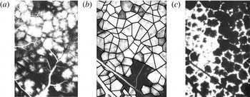
Angiograms performed on monkeys and humans have revealed that the choriocapillaris is functionally composed of a juxtaposition of independent vascular units called lobules, which can be seen in figure 2 (Hayreh Reference Hayreh1974a
, Reference Hayreh1975; Hirata et al.
Reference Hirata, Nishiwaki, Miura, Ieki, Honda, Yumikake, Sugino and Okazaki2004; Fujiwara, Iida & Kanda Reference Fujiwara, Iida and Kanda2007). Lobules typically measure
 $400{-}600~{\rm\mu}\text{m}$
in the macular area. Each lobule is filled independently by a central feeding arteriole (figure 2
a) and drained by a ring collecting venules circumferentially placed around the arteriole (figure 2
c) (Torczynski & Tso Reference Torczynski and Tso1976). Venular openings are shared by neighbouring lobules, and as a result lobules tessellate. The edges between lobules correspond to separatrices, where the residence time of the fluid element is long, rather than physical barriers between adjacent lobules. The boundaries between lobules can therefore be inferred from the regions in which the dye filling and draining times are prolonged, as illustrated in figure 2(b), where the edges were added as a series of connected black lines. The choriocapillaris lacks any active autoregulation (Bill Reference Bill1962; Friedman Reference Friedman1970; Armaly & Araki Reference Armaly and Araki1974; Gherezguiher, Okubo & Koss Reference Gherezguiher, Okubo and Koss1991), and the filling and draining patterns observed in figure 2 are solely determined by the differences in pressure between feeding and draining vessels (Flower, Fryczkowski & McLeod Reference Flower, Fryczkowski and McLeod1995).
Fluorescein angiogram of the choriocapillaris, taken with permission from Hayreh (Reference Hayreh1974b ) (the scale bars are missing from the original publication). The fluorescent dye injected in the general circulation begins to appear in the choriocapillaris in (a), revealing the lobular organisation. Each lobule is filled through the arteriolar opening located at its centre. The number of lobules illuminated is maximal a few seconds later, as shown in (b), where the boundary between lobules has been added as a series of connected black lines. The dye is then evacuated through the periphery of the lobules, as shown in (c).

The anatomical organisation of the choriocapillaris changes dramatically over the eye globe. The average capillary and septae diameter increases further from the macula (Salzman Reference Salzman1912; Hogan & Feeney Reference Hogan and Feeney1961; Garron Reference Garron1963; Klien Reference Klien1966; Hogan et al.
Reference Hogan, Alvarado and Weddell1971; Fryczkowski et al.
Reference Fryczkowski, Sherman and Walker1991). The fraction of the volume occupied by the capillaries over lobules – or vascular volume fraction – varies from 0.75 in the macula to 0.5 at the equator (Ramrattan et al.
Reference Ramrattan, van der Schaft, Mooy, de Bruijn, Mulder and de Jong1994; Spraul et al.
Reference Spraul, Lang, Grossniklaus and Lang1999, Reference Spraul, Lang, Lang and Grossniklaus2002). In ageing, the vascular volume fraction can fall to as little as 0.4 in the macular area (Ramrattan et al.
Reference Ramrattan, van der Schaft, Mooy, de Bruijn, Mulder and de Jong1994). The density of servicing vessels decreases steadily from the macula to the periphery (Amalric Reference Amalric1983; Fryczkowski et al.
Reference Fryczkowski, Sherman and Walker1991; Fryczkowski Reference Fryczkowski1994), while the average distance between these vessels increases. As a result, the average dimension of lobules increases from 400–
 $600~{\rm\mu}\text{m}$
close to the macula to
 $500{-}1100~{\rm\mu}\text{m}$
in the periphery (Yoneya & Tso Reference Yoneya and Tso1987; Fryczkowski et al.
Reference Fryczkowski, Sherman and Walker1991; Fryczkowski Reference Fryczkowski1994; Hirata et al.
Reference Hirata, Nishiwaki, Miura, Ieki, Honda, Yumikake, Sugino and Okazaki2004; Fujiwara et al.
Reference Fujiwara, Iida and Kanda2007).
The purpose of the present study is to describe the flow dynamics and the transport of corpuscles within the choriocapillaris as a first step towards understanding its physiology. Therefore, the diffusion of species through the capillary vessel walls and filtration is not investigated here. Blood consists of a suspension of corpuscles, among which erythrocytes, which account for 99 % of them, are the main agents for transporting oxygen. Since choriocapillaris vessels are less than
 $300~{\rm\mu}\text{m}$
in diameter, the blood flow is subject to the Farhæus effect, whereby the average velocity of erythrocytes is higher than that of the plasma (Fahraeus Reference Fahraeus1929). This effect is axisymmetric and can be averaged over the vessel cross-section.
Modelling of the blood flow in the choriocapillaris has to the best of our knowledge only been attempted once before, by Flower et al. (Reference Flower, von Kerczek, Zhu, Ernest, Eggleton and Topoleski2001), in order to determine the effect of photocoagulation on the blood flow in the choriocapillaris and in a choroidal neovascularisation, which is an area where new pathological vessels develop as a result of AMD. The choriocapillaris was modelled as an infinite thin porous layer of uniform thickness. The drag coefficient and the Darcy permeability of the porous layer were calculated using the theoretical solution for the viscous flow in a channel with periodic cross-bridging fibres developed by Tsay & Weinbaum (Reference Tsay and Weinbaum1991). However, the geographical variations in the choriocapillaris anatomy and the lobular nature of the choriocapillaris were not taken into account.
In this paper, the study of the blood flow is restricted to the elementary domains that lobules form. Lobules are modelled as tessellating polygonal prisms, whose axial height is much smaller than their width. The septae are modelled as cylinders of constant diameter placed with their axes parallel to the axis of the prism and spanning its height that are randomly placed in the domain according to a uniform probability distribution. The Reynolds number of the blood flow is of the order of
 $10^{-1}$
so that the flow is viscously dominated, and this approximation is applied. The flow is simplified by approximating the geometry as a thin parallel-walled gap or Hele-Shaw cell, where the height of the channel is much smaller than the diameter of the cylinders and the component of the blood flow perpendicular to the plates is neglected.
The slow flow of an incompressible viscous fluid around cylindrical bodies confined between two parallel plates has attracted considerable interest in a variety of fields. Hele-Shaw (Reference Hele-Shaw1898) was the first to observe that the streamlines of a viscous fluid flowing around cylindrical obstacles emulate the lines of forces around metallic cylinders placed in a dielectric medium in a magnetic field. This observation found mathematical ground with Stokes, who proved that the full Stokes flow equations describing the flow can be replaced by the potential flow equation everywhere except for within a boundary layer region at the cylinders. Thompson (Reference Thompson1968) later showed that this boundary layer has a width of
 $O(h)$
, where
 $h$
is the distance between the two parallel plates, and that within this boundary layer the perpendicular component of the fluid velocity cannot be neglected. Later, Balsa (Reference Balsa1998) showed that this boundary layer contains a streamwise vorticity generated at the cylinder and channel walls. The extensive application of Hele-Shaw flows in a variety of physiology-related problems led to further advances in their analysis, see for instance Lee & Fung (Reference Lee and Fung1969), Tsay & Weinbaum (Reference Tsay and Weinbaum1991), Zheng & Weinbaum (Reference Zheng and Weinbaum1994) and Wei et al. (Reference Wei, Waters, Liu and Grotberg2003). In most studies, the Hele-Shaw analysis is carried out under the assumption of uniform flows. In the present work, the flow is set by radial inlets and outlets and is as a result non-uniform. Radial flows have so far mostly been studied in the context of radial fingering in free boundaries (Richardson Reference Richardson1972; Paterson Reference Paterson1981).
In the present study, a two-dimensional analysis of the Hele-Shaw flow around cylindrical bodies is carried out within a bounded polygonal domain. The flow is driven by a single inlet with a prescribed radially outward flow and a zero-pressure boundary condition at the outlets, which are located at the vertices of the polygon. The pressure drop and the fluid particle residence time are the two diagnostic tools used in this model. The pressure drop characterises the perfusion of the vascular bed. The variations observed in the anatomy of the choriocapillaris and during angiography suggest that it varies significantly over the eye globe, and that it could therefore be a determinant of the local architecture of the capillary bed. The fluid particle residence time provides a metric of the transport of corpuscles in the choriocapillaris and of the homogeneity of this transport within lobules. It also describes the blood renewal rate and nutrient turnover time, which may be impaired in the pathogenesis of AMD. The concentration of arteriolar and venular openings, the average distance between arterioles and venules feeding and draining the capillary bed, and the vascular volume fraction are the three spatially varying characteristics of the choriocapillaris over the eye globe; therefore, the pressure drop and the residence time were calculated for a range of these parameters.
This paper is structured as follows. In § 2, the modelling assumptions for the rheology of blood and the flow geometry are described and justified. After defining the equations for the flow and the diagnostic tools, the pressure drop and residence time are defined and analysed. In § 3, an analytical solution for the equations describing the flow is calculated and asymptotic approximations are formulated when the cylinders are absent. In § 4, the effect of the cylinders on the pressure drop and residence time is investigated numerically and analytically.
2. Mathematical model
2.1. Modelling assumption and justification
2.1.1. Rheology of blood
Blood is composed of a plasma suspension of cells. Erythrocytes account for 99 % of these living cells and are therefore the main determinant of its mechanical properties. In capillaries of less than
 $300~{\rm\mu}\text{m}$
in diameter, erythrocytes deform and align with the flow, while a plasma layer forms along the capillary wall. This results in a reduction of frictional losses and of the volume percentage of erythrocytes in blood – or haematocrit – which causes a decrease of the effective blood viscosity (Fahraeus Reference Fahraeus1929). In these capillaries, blood displays Newtonian characteristics, and has a haematocrit-dependent viscosity (Replogle, Meiselman & Merrill Reference Replogle, Meiselman and Merrill1967; Pries et al.
Reference Pries, Secomb, Gessner, Sperandio, Gross and Gaehtgens1994). Here, blood is modelled as a Newtonian fluid. The blood viscosity is calculated with an empirical formula from the literature describing the linkage between viscosity and haematocrit (Pries et al.
Reference Pries, Secomb, Gessner, Sperandio, Gross and Gaehtgens1994). The haematocrit is taken to be the one of blood leaving lobules, measured as 15–20 % in rat choroidal venules (Braun, Dewhirst & Hatchell Reference Braun, Dewhirst and Hatchell1997). The blood density is taken to be constant and equal to
 ${\it\rho}=1040~\text{g}~\text{l}^{-1}$
.
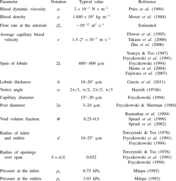
A list of physiological parameters along with typical values is provided in table 1.
List of physiological parameters characterising the geometry and fluid properties of a choriocapillaris lobule. When a range of values is given, the value used is marked with an asterisk. The flow rate at the arteriole was estimated from the average capillary blood velocity and the radius of the inlets. The vertex angle was approximated from angiography images.

2.1.2. Geometry
Functionally, choriocapillaris lobules form thin interfaces characterised by a span of
 $400{-}800~{\rm\mu}\text{m}$
and a thickness of
 $10{-}20~{\rm\mu}\text{m}$
; their aspect ratio is high, of the order of 0.01. As seen in figure 2, lobules are filled from the centre by an arteriole connected at a right angle relative to the plane of the capillaries and drained by a ring of collecting venules located at the vertices of the lobules and connected in a similar fashion. Each venule drains adjacent lobules so that lobular shapes tessellate. The shape of lobules is set by the distribution of draining venules around the arteriolar supply. The regularity of the edges observed in figure 2(b) suggests that the pressure at arterioles and venules is relatively stable over small clusters of lobules. The pressure at the outlets is taken to be the same. The flow at the inlets and outlets is assumed to be uniform and axisymmetric. This is an idealisation of the physiology, as the perfusion over lobules may not be uniform, and different regions may not receive the same supply of blood. The separation between lobules is formed by separatrices of the flow, on which the fluid residence time is long. These separatrices are approdimated by straight lines.
Anatomically, one of the most distinctive features of choriocapillaris vessels is their characteristic flatness; their width can be up to six times larger than their thickness. They form a highly redundant capillary bed, as a variety of paths can be taken to connect any two points. Functionally, however, blood can reach a particular point through one path only, which is determined by the pressure differences between feeding and draining vessels, and the position of the septae. As the void volume fraction, which is the volume fraction occupied by the septae within lobules – and is therefore equal to one minus the vascular volume fraction – is high, between 0.25 and 0.5, a continuum approach is implemented here.
As a result, choriocapillaris lobules are modelled as tessellating polygonal prisms supplied and drained by inlets and outlets connecting to their lower surface perpendicularly to the plane of the capillaries. The inlet is located inside the lobular domain, while the outlets are placed at the vertices of the prisms. The septae are modelled as cylinders of constant diameter
 $2a$
randomly distributed over lobules following a uniform distribution. These polygonal prisms can be decomposed into elementary tessellating triangular prisms with a source at their vertex and a sink at the remaining two vertices.
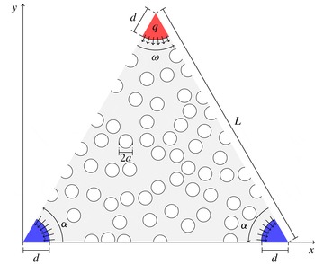
Here, the blood flow is investigated in two dimensions over these elementary triangular domains (see figure 3). The geometry is idealised by taking the triangles to be isosceles. Since they represent a portion of a polygon, the velocity is continuous over the triangle walls, and a non-flux condition is applied. The triangle is characterised by a vertex angle
 ${\it\omega}$
(when more convenient, the angle at the base
 ${\it\alpha}={\rm\pi}/2-{\it\omega}/2$
is used), and a side length
 $L$
. As a result of the variation in the lobular shapes over the choriocapillaris observed in figure 2,
 ${\it\omega}$
varies over the eye globe. The radius
 $d$
of the inlets and outlets is taken to be the same. The fraction of the lobular volume occupied by the cylinders is the void fraction
 ${\it\Phi}$
and is defined as
 $$\begin{eqnarray}{\it\Phi}=\frac{1}{\mathscr{A}_{t}}\mathop{\sum }_{i=1}^{N}\mathscr{A}_{i},\end{eqnarray}$$
where
 $\mathscr{A}_{i}$
is the area of each cylinder labelled
 $i=1,2,\dots ,N$
and
 $\mathscr{A}_{t}$
is the area of the triangle minus the area taken by the inlets and outlets,
 $\mathscr{A}_{t}=(L^{2}\sin 2{\it\alpha})/2-{\rm\pi}d^{2}/2=(L^{2}\sin {\it\omega})/2-{\rm\pi}d^{2}/2$
. In order to generate the cylinder array, a dart-throwing algorithm was implemented to create a Poisson-disk distribution with a preset minimal distance between cylinders.
The flow is studied in an isosceles triangle
 ${\it\Omega}$
characterised by a vertex angle
 ${\it\omega}$
and a side length
 $L$
. One inlet and two outlets are placed at its vertices. The choriocapillaris septae are modelled by cylinders of constant diameter
 $2a$
randomly distributed over the triangle. A prescribed area flux into the triangular domain
 $q$
is imposed at the inlet. A zero-pressure boundary condition is imposed at the outlets.

2.2. Defining equations
Blood is modelled as an incompressible Newtonian fluid with a uniform density and viscosity. The flow is described by the conservation of momentum and mass
 $$\begin{eqnarray}\displaystyle & {\it\rho}(\boldsymbol{u}\boldsymbol{\cdot }\boldsymbol{{\rm\nabla}})\boldsymbol{u}=-\boldsymbol{{\rm\nabla}}p+{\it\mu}{\rm\nabla}^{2}\boldsymbol{u}, & \displaystyle\end{eqnarray}$$
 $$\begin{eqnarray}\displaystyle & \boldsymbol{{\rm\nabla}}\boldsymbol{\cdot }\boldsymbol{u}=0, & \displaystyle\end{eqnarray}$$
 $$\begin{eqnarray}\boldsymbol{u}=\frac{Q}{{\rm\pi}d^{2}}\widehat{\boldsymbol{z}}\end{eqnarray}$$
at the inlet, which consists of a uniform inflow perpendicular to the plane of the triangular prism characterised by a flow rate entering the triangular domain
 $Q$
. Denoting by
 $\mathscr{Q}_{a}$
the flow rate at the arteriole supplying the lobule, which is assumed to be axisymmetric,
 $Q$
satisfies
 $$\begin{eqnarray}Q=\frac{{\it\omega}}{2{\rm\pi}}\mathscr{Q}_{a}.\end{eqnarray}$$
At the walls, since the triangular prism represents the element of symmetry of a lobule, the velocity is continuous over the boundary between adjacent triangles, and a slip condition is applied, i.e.
 $$\begin{eqnarray}\frac{\partial \boldsymbol{u}}{\partial n}\boldsymbol{\cdot }\hat{\boldsymbol{n}}=0,\end{eqnarray}$$
where
 $\hat{\boldsymbol{n}}$
is a unit vector perpendicular to the wall surface. The pressure at the outlets is constant, and for simplicity is taken to be zero. The boundary condition
 $\boldsymbol{u}=\mathbf{0}$
is imposed on the planes
 $z=0$
and
 $z=h$
and over the internal geometry.
From table 1, the blood velocity in the choriocapillaris is of the order of
 $2~\text{mm}~\text{s}^{-1}$
. The Reynolds number for the flow in the choriocapillaris is of the order of
 $\mathit{Re}\sim 0.1$
. The flow is characterised by
 $\mathit{Re}(h/2L)^{2}\sim 10^{-5}$
, which is significantly smaller than unity, so that a lubrication approximation can be applied to simplify the momentum equation (Reynolds Reference Reynolds1886), i.e.
 $$\begin{eqnarray}-\boldsymbol{{\rm\nabla}}_{h}p+{\it\mu}\frac{\partial ^{2}\boldsymbol{u}}{\partial z^{2}}=\mathbf{0},\end{eqnarray}$$
where
 $$\begin{eqnarray}\boldsymbol{{\rm\nabla}}_{h}=\left(\frac{\partial }{\partial x},\frac{\partial }{\partial y},0\right).\end{eqnarray}$$
Imposition of the continuity of mass (2.3) and the boundary conditions
 $\boldsymbol{u}=\mathbf{0}$
on
 $z=0$
and
 $z=h$
leads to
 $$\begin{eqnarray}{\rm\nabla}_{h}^{2}p=\mathbf{0}.\end{eqnarray}$$
On defining the average local velocity in the plane of the choriocapillaris as
 $$\begin{eqnarray}\boldsymbol{u}_{h}=\frac{1}{h}\int _{0}^{h}\boldsymbol{u}\,\text{d}z\cdot (1,1,0),\end{eqnarray}$$
the momentum equation reduces to
 $$\begin{eqnarray}\boldsymbol{u}_{h}=-\frac{h^{2}}{12{\it\mu}}\boldsymbol{{\rm\nabla}}_{h}p=-\frac{K}{{\it\mu}}\boldsymbol{{\rm\nabla}}_{h}p,\end{eqnarray}$$
where
 $K=h^{2}/12$
is the permeability characterising the flow between parallel plates. At the inlet, a radial source flow is imposed, and the velocity
 $\boldsymbol{u}_{h}$
satisfies
 $$\begin{eqnarray}\int _{-{\it\omega}/2}^{{\it\omega}/2}u_{h}d\,\text{d}{\it\theta}=q,\end{eqnarray}$$
where
 $$\begin{eqnarray}q=\frac{Q}{h}=\frac{{\it\omega}\mathscr{Q}_{a}}{2{\rm\pi}h}\end{eqnarray}$$
is the area flux into the triangular domain. As a result, the inlet boundary condition becomes
 $$\begin{eqnarray}\boldsymbol{u}_{h}=\frac{q}{{\it\omega}d}\hat{\boldsymbol{r}},\end{eqnarray}$$
where
 $\hat{\boldsymbol{r}}$
is the unit radial vector; on the outlets
 $p=0$
is applied. On the surface of the posts and on the upper and lower walls of the prism, the kinematic boundary condition is applied:
 $$\begin{eqnarray}\boldsymbol{u}_{h}\boldsymbol{\cdot }\hat{\boldsymbol{n}}=0,\end{eqnarray}$$
where
 $\hat{\boldsymbol{n}}$
is the normal to the surface of the walls or cylinders. At the side walls, the slip condition (2.6) becomes
 $$\begin{eqnarray}\frac{\partial \boldsymbol{u}_{h}}{\partial n}\boldsymbol{\cdot }\hat{\boldsymbol{n}}=0.\end{eqnarray}$$
Within a distance
 $O(h)$
of the edge of the cylinders, inlet and outlets, the flow is out of the plane of the choriocapillaris. The impact on the global flow is minimal.
All of the lengths are scaled relative to the triangle side length
 $L$
, and non-dimensional measures are written with a tilde. The ratio of the inlet radius to the lobule span is denoted
 $d/L={\it\delta}$
and is kept constant for all the calculations. The velocity
 $\boldsymbol{u}_{h}$
is made dimensionless with respect to the velocity of the emerging flow
 $\bar{U}=q/L$
and the pressure
 $p$
with respect to the characteristic viscous stress
 ${\it\mu}\bar{U}L/K$
. Denoting by
 $\tilde{\boldsymbol{u}}_{h}$
the non-dimensional average local velocity and by
 $\tilde{p}$
the non-dimensional pressure, the equations for the flow (2.9) and (2.11) become
 $$\begin{eqnarray}\displaystyle & \tilde{\boldsymbol{u}}_{h}=-\tilde{\boldsymbol{{\rm\nabla}}}_{h}~\tilde{p}, & \displaystyle\end{eqnarray}$$
 $$\begin{eqnarray}\displaystyle & \tilde{{\rm\nabla}}_{h}^{2}~\tilde{p}=0. & \displaystyle\end{eqnarray}$$
2.3. Diagnostic tools
The blood flow through the choriocapillaris is set by the pressure drop between inlets and outlets. It is defined here as an average over the inlet surface,
 $$\begin{eqnarray}{\rm\Delta}\tilde{p}=\frac{1}{\tilde{S}}\int _{\mathit{inlet}}\tilde{p}\,\text{d}\tilde{S},\end{eqnarray}$$
where
 $\tilde{S}$
denotes the inlet surface.
The residence or travel time describes the time spent by a fluid particle, released at the inlet, in the choriocapillaris lobule. Corpuscles are assumed to be symmetrically distributed over the cross-section of a lobule and to travel at the depth averaged velocity
 $\tilde{\boldsymbol{u}}_{h}$
. The residence time of a fluid particle released at an angle
 ${\it\theta}$
from the inlet surface and advected to an outlet by the velocity field
 $\tilde{\boldsymbol{u}}_{h}$
is
 $$\begin{eqnarray}{\rm\Delta}\tilde{T}({\it\theta})=\int _{\tilde{S}}\frac{\text{d}\tilde{s}}{|\tilde{\boldsymbol{u}}_{h}|},\end{eqnarray}$$
where the integral is taken along a streamline. As a result of the geometry, the domain contains a saddle point characterised by a zero shear stress at the separation point between the streamlines (Hunt et al.
Reference Hunt, Abell, Peterka and Woo1978). A stagnation streamline connects the inlet to the saddle point. On the stagnation streamline, the fluid particle residence time is infinite. It will be shown in § 3.2 that adjacent to the stagnation streamline, the residence time has a logarithmic dependence on the angle at the source
 ${\it\theta}$
, and that this singularity is integrable so that the average residence time, defined as
 $$\begin{eqnarray}\langle \tilde{T}\rangle =\frac{1}{{\it\omega}}\int _{-{\it\omega}/2}^{{\it\omega}/2}{\rm\Delta}\tilde{T}({\it\theta})\,\text{d}{\it\theta},\end{eqnarray}$$
is finite and can be estimated from the average of all the travel times of particles released on the inlet. In order to assess the magnitude of the residence time distribution, the root of the mean square of the residence time distribution, expressed as
 $$\begin{eqnarray}\langle \tilde{T}\rangle _{RMS}=\sqrt{\frac{1}{{\it\omega}}\int _{-{\it\omega}/2}^{{\it\omega}/2}({\rm\Delta}\tilde{T}({\it\theta})-\langle \tilde{T}\rangle )^{2}\,\text{d}{\it\theta}},\end{eqnarray}$$
is used.
3. Analytical results and approximate models for
 ${\it\Phi}=0$

The aim of this section is to characterise the dependence of the flow, pressure drop and residence time on the angle at the inlet
 ${\it\omega}$
for
 ${\it\Phi}=0$
. A conformal mapping is first described. The singularity in residence time in the vicinity of the stagnation streamline is then characterised. Asymptotic approximations are thereafter developed for both
 $|{\it\omega}|\ll 1$
and
 $|{\rm\pi}-{\it\omega}|\ll 1$
.
3.1. Analytical resolution by conformal mapping
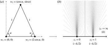
An analytical solution is sought by mapping the potential created by one source and two sinks located on the real axis onto a triangle (see figure 4). The following analysis is carried out on the complex plane, with the correspondence
 $w=(x,y)\rightarrow z=x+\text{i}y=r\text{e}^{\text{i}{\it\theta}}$
, where
 $r$
and
 ${\it\theta}$
are respectively the modulus and argument of
 $z$
. The conformal map of the upper half-complex-plane
 $D$
onto the isosceles triangle
 ${\it\Omega}$
is built by using the Schwartz–Christoffel formula:
 $$\begin{eqnarray}f(z)=a_{0}+a_{1}\int _{}^{z}({\it\zeta}-z_{1})^{({\it\alpha}/{\rm\pi})-1}({\it\zeta}-z_{2})^{({\it\alpha}/{\rm\pi})-1}\,\text{d}{\it\zeta},\end{eqnarray}$$
where
 $a_{0}$
and
 $a_{1}$
are two complex constants and the images of the points
 $z_{1}=0$
and
 $z_{2}=1$
are the triangle vertices
 $w_{1}=0$
and
 $w_{2}=2\cos {\it\alpha}$
(see figure 4). The third vertex
 $w_{3}$
is taken to be the image of infinity on the real axis
 $z_{3}\rightarrow \infty$
. The conformal map is
 $$\begin{eqnarray}f(z)=2\cos {\it\alpha}~\mathscr{I}\left(z,\frac{{\it\alpha}}{{\rm\pi}},\frac{{\it\alpha}}{{\rm\pi}}\right),\end{eqnarray}$$
where
 $\mathscr{I}$
is the regularised incomplete beta function (Nehari Reference Nehari1952). The map f is analytic on
 $D$
and admits an inverse function
 $g=f^{-1}$
, which maps the triangular domain
 ${\it\Omega}$
back onto the transformed plane
 $D$
. The inverse map
 $g$
is expressed as
 $$\begin{eqnarray}g(z)=\mathscr{I}^{-1}\left(\frac{z}{2\cos {\it\alpha}},\frac{{\it\alpha}}{{\rm\pi}},\frac{{\it\alpha}}{{\rm\pi}}\right),\end{eqnarray}$$
where
 $\mathscr{I}^{-1}$
is the inverse regularised incomplete beta function.
The Schwarz–Christoffel conformal map is calculated to transform the triangular domain in (a) into the half-plane in (b). In (b), the source of strength
 $k$
, sinks of strength
 $-k/2$
and representative streamlines are shown. (a) Real plane (
 ${\it\omega}$
), (b) transformed plane (D).

Since the pressure
 $\tilde{p}$
satisfies Laplace’s equation, it is harmonic on the triangular domains
 ${\it\Omega}$
and is the real part of a complex harmonic function
 ${\it\chi}$
:
 $$\begin{eqnarray}{\it\chi}(z)={\it\phi}(x,y)+\text{i}{\it\psi}(x,y)=-\tilde{p}(x,y)+\text{i}{\it\psi}(x,y),\end{eqnarray}$$
where
 ${\it\chi}$
is the complex pressure potential,
 ${\it\phi}$
is the velocity potential and
 ${\it\psi}$
is the streamfunction. The complex potential
 ${\it\chi}$
is calculated by conformally mapping the potential, denoted
 ${\it\chi}_{D}$
, created by the sources and sinks located at the images
 $z_{i}=g(w_{i})$
in
 $D$
onto
 ${\it\Omega}$
. The complex potential generated in
 $D$
by a fluid emerging at a rate per unit length
 $k$
by a source located at
 $z=z_{3}$
and disappearing at the two sinks of equal strength
 $k/2$
located at
 $z=0$
and
 $z=1$
is
 $$\begin{eqnarray}{\it\chi}_{D}(z)=k\log \frac{z-z_{3}}{\sqrt{z(z-1)}}.\end{eqnarray}$$
The complex potential in the real plane is therefore
 $$\begin{eqnarray}{\it\chi}(z)={\it\chi}_{D}(g(z))=k\log \frac{g(z)-z_{3}}{\sqrt{g(z)(g(z)-1)}},\end{eqnarray}$$
or, using the analytical expression of
 $g$
,
 $$\begin{eqnarray}{\it\chi}(z)=k\log \frac{\left(\mathscr{I}^{-1}\left(\displaystyle \frac{z}{2\cos {\it\alpha}},\frac{{\it\alpha}}{{\rm\pi}},\frac{{\it\alpha}}{{\rm\pi}}\right)-z_{3}\right)}{\sqrt{\mathscr{I}^{-1}\left(\displaystyle \frac{z}{2\cos {\it\alpha}},\frac{{\it\alpha}}{{\rm\pi}},\frac{{\it\alpha}}{{\rm\pi}}\right)\left(\mathscr{I}^{-1}\left(\displaystyle \frac{z}{2\cos {\it\alpha}},\frac{{\it\alpha}}{{\rm\pi}},\frac{{\it\alpha}}{{\rm\pi}}\right)-1\right)}}.\end{eqnarray}$$
The complex velocity is
 $$\begin{eqnarray}\displaystyle {\it\upsilon}(z) & = & \displaystyle \frac{\text{d}{\it\chi}}{\text{d}z}=-k\frac{{\it\beta}\left(\displaystyle \frac{{\it\alpha}}{{\rm\pi}},\frac{{\it\alpha}}{{\rm\pi}}\right)}{4\cos {\it\alpha}}\left\{(2z_{3}-1)\mathscr{I}^{-1}\left(\displaystyle \frac{z}{2\cos {\it\alpha}},\frac{{\it\alpha}}{{\rm\pi}},\frac{{\it\alpha}}{{\rm\pi}}\right)-z_{3}\right\}\nonumber\\ \displaystyle & & \displaystyle \times \,\left\{\left(\mathscr{I}^{-1}\!\left(\displaystyle \frac{z}{2\cos {\it\alpha}},\frac{{\it\alpha}}{{\rm\pi}},\frac{{\it\alpha}}{{\rm\pi}}\right)-z_{3}\right)\!\!\left[\left(1-\mathscr{I}^{-1}\left(\displaystyle \frac{z}{2\cos {\it\alpha}},\frac{{\it\alpha}}{{\rm\pi}},\frac{{\it\alpha}}{{\rm\pi}}\right)\!\right)\right.\right.\nonumber\\ \displaystyle & & \displaystyle \left.\left.\times \,\mathscr{I}^{-1}\!\left(\displaystyle \frac{z}{2\cos {\it\alpha}},\frac{{\it\alpha}}{{\rm\pi}},\frac{{\it\alpha}}{{\rm\pi}}\right)\right]^{{\it\alpha}/{\rm\pi}}\right\}^{-1},\end{eqnarray}$$
where
 ${\it\beta}$
is the beta function. Since
 $\mathscr{I}^{-1}$
is bounded on
 ${\it\Omega}$
for
 ${\it\delta}>0$
, the limit of
 ${\it\upsilon}$
when
 $z_{3}\rightarrow \infty$
can be calculated:
 $$\begin{eqnarray}{\it\upsilon}(z)=k\frac{{\it\beta}\left(\displaystyle \frac{{\it\alpha}}{{\rm\pi}},\frac{{\it\alpha}}{{\rm\pi}}\right)}{4\cos {\it\alpha}}\frac{2\mathscr{I}^{-1}\left(\displaystyle \frac{z}{2\cos {\it\alpha}},\frac{{\it\alpha}}{{\rm\pi}},\frac{{\it\alpha}}{{\rm\pi}}\right)-1}{\left[\left(1-\mathscr{I}^{-1}\left(\displaystyle \frac{z}{2\cos {\it\alpha}},\frac{{\it\alpha}}{{\rm\pi}},\frac{{\it\alpha}}{{\rm\pi}}\right)\right)\mathscr{I}^{-1}\left(\displaystyle \frac{z}{2\cos {\it\alpha}},\frac{{\it\alpha}}{{\rm\pi}},\frac{{\it\alpha}}{{\rm\pi}}\right)\right]^{{\it\alpha}/{\rm\pi}}}.\end{eqnarray}$$
The value of
 $k$
is determined by imposing the boundary condition at the inlet
 $$\begin{eqnarray}\displaystyle \int _{{\rm\pi}+{\it\alpha}}^{2{\rm\pi}-{\it\alpha}}|{\it\upsilon}(\text{e}^{\text{i}{\it\alpha}}+{\it\delta}\text{e}^{\text{i}{\it\theta}})|\,\text{d}{\it\theta}=\int _{{\rm\pi}+{\it\alpha}}^{2{\rm\pi}-{\it\alpha}}|\tilde{\boldsymbol{u}}_{h}|_{z=\text{e}^{\text{i}{\it\alpha}}+{\it\delta}\text{e}^{\text{i}{\it\theta}}}\,\text{d}{\it\theta}.\end{eqnarray}$$
The right-hand side of (3.10) can be rewritten as
 $$\begin{eqnarray}\displaystyle \int _{{\rm\pi}+{\it\alpha}}^{2{\rm\pi}-{\it\alpha}}|\tilde{\boldsymbol{u}}_{h}|\,\text{d}{\it\theta} & = & \displaystyle \frac{1}{{\it\omega}}\displaystyle \int _{{\rm\pi}+{\it\alpha}}^{2{\rm\pi}-{\it\alpha}}\left|\frac{1}{\cos {\it\alpha}+{\it\delta}\cos {\it\theta}+\text{i}(\sin {\it\alpha}+{\it\delta}\sin {\it\theta})}\right|\,\text{d}{\it\theta}\nonumber\\ \displaystyle & = & \displaystyle \frac{2}{{\it\omega}(1+{\it\delta})}\left(\mathscr{F}_{1}\left({\rm\pi}-{\it\alpha}\left|\frac{4{\it\delta}}{(1+{\it\delta})^{2}}\right.\right)-\mathscr{F}_{1}\left(\frac{{\rm\pi}}{2}\left|\frac{4{\it\delta}}{(1+{\it\delta})^{2}}\right.\right)\right),\qquad\end{eqnarray}$$
where
 $\mathscr{F}_{1}$
is the elliptic integral of the first kind (Abramowitz & Stegun Reference Abramowitz and Stegun1972). The value of
 $k$
is therefore
 $$\begin{eqnarray}\displaystyle k & = & \displaystyle \frac{8\cos {\it\alpha}}{{\it\beta}\left(\displaystyle \frac{{\it\alpha}}{{\rm\pi}},\frac{{\it\alpha}}{{\rm\pi}}\right){\it\omega}(1+{\it\delta})}\nonumber\\ \displaystyle & & \displaystyle \times \,\frac{\mathscr{F}_{1}\left(\displaystyle {\rm\pi}-{\it\alpha}\left|\frac{4{\it\delta}}{(1+{\it\delta})^{2}}\right.\right)-\mathscr{F}_{1}\left(\displaystyle \frac{{\rm\pi}}{2}\left|\frac{4{\it\delta}}{(1+{\it\delta})^{2}}\right.\right)}{\displaystyle \int _{{\rm\pi}+{\it\alpha}}^{2{\rm\pi}-{\it\alpha}}\left|\frac{\displaystyle 2\mathscr{I}^{-1}\left(\frac{\text{e}^{\text{i}{\it\alpha}}+{\it\delta}\text{e}^{\text{i}{\it\theta}}}{2\cos {\it\alpha}},\frac{{\it\alpha}}{{\rm\pi}},\frac{{\it\alpha}}{{\rm\pi}}\right)-1}{\displaystyle \left[\left(1-\mathscr{I}^{-1}\!\left(\frac{\text{e}^{\text{i}{\it\alpha}}+{\it\delta}\text{e}^{\text{i}{\it\theta}}}{2\cos {\it\alpha}},\frac{{\it\alpha}}{{\rm\pi}},\frac{{\it\alpha}}{{\rm\pi}}\right)\!\right)\!\mathscr{I}^{-1}\!\left(\displaystyle \frac{\text{e}^{\text{i}{\it\alpha}}+{\it\delta}\text{e}^{\text{i}{\it\theta}}}{2\cos {\it\alpha}},\frac{{\it\alpha}}{{\rm\pi}},\frac{{\it\alpha}}{{\rm\pi}}\right)\!\right]^{{\it\alpha}/{\rm\pi}}}\right|\,\text{d}{\it\theta}}.\nonumber\\ \displaystyle & & \displaystyle\end{eqnarray}$$
The pressure
 $-\tilde{p}$
over
 ${\it\Omega}$
is the real part of
 ${\it\chi}$
, and is expressed as
 $$\begin{eqnarray}\tilde{p}(x,y)=-k\log \left|\frac{\left(\mathscr{I}^{-1}\left(\displaystyle \frac{x+\text{i}y}{2\cos {\it\alpha}},\frac{{\it\alpha}}{{\rm\pi}},\frac{{\it\alpha}}{{\rm\pi}}\right)-z_{3}\right)}{\sqrt{\mathscr{I}^{-1}\left(\displaystyle \frac{x+\text{i}y}{2\cos {\it\alpha}},\frac{{\it\alpha}}{{\rm\pi}},\frac{{\it\alpha}}{{\rm\pi}}\right)\left(\mathscr{I}^{-1}\left(\displaystyle \frac{x+\text{i}y}{2\cos {\it\alpha}},\frac{{\it\alpha}}{{\rm\pi}},\frac{{\it\alpha}}{{\rm\pi}}\right)-1\right)}}\right|.\end{eqnarray}$$
The pressure drop is calculated by subtracting the average pressure over the inlet and over an outlet. The streamfunction
 ${\it\psi}$
is given by the argument of
 ${\it\chi}$
, so that the residence time over a streamline is expressed as
 $$\begin{eqnarray}\displaystyle {\rm\Delta}\tilde{T}({\it\theta}) & = & \displaystyle \frac{4\cos {\it\alpha}}{k{\it\beta}\left(\displaystyle \frac{{\it\alpha}}{{\rm\pi}},\frac{{\it\alpha}}{{\rm\pi}}\right)}\nonumber\\ \displaystyle & & \displaystyle \times \,\displaystyle \int _{{\it\psi}_{\tilde{S}}}^{}\frac{\left|\left(1-\mathscr{I}^{-1}\left(\displaystyle \frac{z}{2\cos {\it\alpha}},\frac{{\it\alpha}}{{\rm\pi}},\frac{{\it\alpha}}{{\rm\pi}}\right)\right)\mathscr{I}^{-1}\left(\displaystyle \frac{z}{2\cos {\it\alpha}},\frac{{\it\alpha}}{{\rm\pi}},\frac{{\it\alpha}}{{\rm\pi}}\right)\right|^{{\it\alpha}/{\rm\pi}}}{\left|2\mathscr{I}^{-1}\left(\displaystyle \frac{z}{2\cos {\it\alpha}},\frac{{\it\alpha}}{{\rm\pi}},\frac{{\it\alpha}}{{\rm\pi}}\right)-1\right|}\,\text{d}\tilde{s}.\qquad\end{eqnarray}$$
The complex potential
 ${\it\chi}$
and the complex velocity
 ${\it\upsilon}$
were calculated by numerically inverting the complex incomplete normalised beta function using the Newton method. The streamlines of the flow, the pressure field and the instant velocity field for two different values of
 ${\it\omega}$
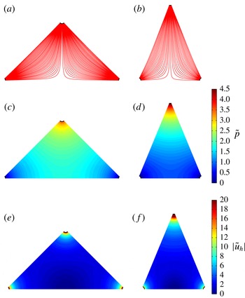
are plotted in figure 5(a–f). They show that the flow within the triangular domain forms a region of transition between a dominantly source flow at the inlet and dominantly sink flows near the outlets. In the vicinity of the stagnation point, the velocity profile becomes quasi-circular as the streamlines separate.
Streamlines of the flow (a,b), pressure field (c,d) and instant velocity profile (e,f) calculated using the conformal mapping solution for
 ${\it\omega}={\rm\pi}/2$
and
 ${\it\omega}={\rm\pi}/4$
respectively. The instant velocity was plotted over a reduced range of values.

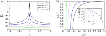
The residence time distribution, plotted in figure 6(a), displays a strong dependence on
 ${\it\omega}$
. When
 $|{\it\omega}/2-{\it\theta}|\ll 1$
, the flow is quasi-parallel, and the residence time distribution is quasi-uniform, as shown by the cumulative density function (c.d.f.) plotted in figure 6(b,c). As the distance from the wall increases, the flow path elongates (see figure 5
a,b). The velocity of the fluid particle decreases in the regions closest to the stagnation point, and the c.d.f. increases exponentially. As
 $|{\it\theta}|\rightarrow 0$
, the residence time diverges. The characterisation of this singularity is sought in the next section.
3.2. Asymptotic analysis of the residence time close to the stagnation point
As the fluid elements travelling along the longest streamlines approach the stagnation point located at
 $z=\cos {\it\alpha}$
, the instant velocity
 $|\tilde{\boldsymbol{u}}_{h}|\rightarrow 0$
, which results in the discontinuity in residence time observed in figure 6(a). This discontinuity can be analysed by performing an asymptotic analysis of the residence time close to the stagnation point. In this region the flow can be modelled by a stagnation point flow described by the complex potential
 ${\it\eta}$
and complex velocity
 ${\it\Upsilon}$
:
 $$\begin{eqnarray}{\it\eta}(z)={\it\gamma}(z-\cos {\it\alpha})^{2},\quad {\it\Upsilon}(z)=2{\it\gamma}(z-\cos {\it\alpha}),\end{eqnarray}$$
where
 ${\it\gamma}$
is a constant. The value of
 ${\it\gamma}$
can be calculated by considering the equipotentials of the instant velocity
 $|{\it\upsilon}|$
close to the stagnation point. If
 $|{\it\epsilon}|\ll 1$
is the distance from the stagnation point, and
 $S_{{\it\epsilon}}$
is the equipotential going through
 ${\it\epsilon}$
(see figure 7
a), then the value for
 ${\it\gamma}$
is
 $$\begin{eqnarray}{\it\gamma}=\frac{\displaystyle \int _{S_{{\it\epsilon}}}^{}|{\it\upsilon}(z)|\,\text{d}s}{2\displaystyle \int _{S_{{\it\epsilon}}}^{}|z-\cos {\it\alpha}|\,\text{d}s}.\end{eqnarray}$$
In the limit where
 $0<{\it\epsilon}\ll 1$
the equipotentials
 $S_{{\it\epsilon}}$
are circular, so that the value for
 ${\it\gamma}$
is
 $$\begin{eqnarray}{\it\gamma}=\frac{1}{2{\rm\pi}{\it\epsilon}}\displaystyle \int _{S_{{\it\epsilon}}}^{}|{\it\upsilon}(z)|\,\text{d}s.\end{eqnarray}$$
Since
 $|{\it\upsilon}|$
depends on
 ${\it\omega}$
,
 ${\it\gamma}$
is a function of the geometry. In the vicinity of the stagnation point it is more convenient to express the velocity using cylindrical coordinates
 $(r^{\prime },{\it\varphi})$
centred on the stagnation point (see figure 7
a). The following description assumes that
 ${\it\theta}\geqslant 0$
, although the case
 ${\it\theta}\leqslant 0$
is symmetrical. At a distance
 $r^{\prime }=O({\it\epsilon})$
from the stagnation point, the radial and angular velocities are respectively
 $$\begin{eqnarray}\tilde{u} _{r}=2{\it\gamma}\tilde{r}^{\prime }\cos 2{\it\varphi},\quad \tilde{u} _{{\it\varphi}}=-2{\it\gamma}\tilde{r}^{\prime }\sin 2{\it\varphi}.\end{eqnarray}$$
The residence time of the fluid elements in the vicinity of the stagnation point is
 $$\begin{eqnarray}{\rm\Delta}\tilde{T}=\frac{1}{2{\it\gamma}}\displaystyle \int _{{\it\psi}_{{\it\epsilon}}}^{}\frac{\text{d}\tilde{s}}{\tilde{r}^{\prime }}.\end{eqnarray}$$
The streamfunction for the flow,
 $$\begin{eqnarray}{\it\psi}(\tilde{r}^{\prime },{\it\varphi})={\it\gamma}\tilde{r}^{\prime 2}\sin 2{\it\varphi},\end{eqnarray}$$
is symmetric relative to the axis
 ${\it\varphi}={\rm\pi}/4$
. As a result, the two intersections of the streamline with the equipotential
 $S_{{\it\epsilon}}$
are
 $$\begin{eqnarray}\tilde{r}_{1}^{\prime }=\frac{{\it\epsilon}^{\prime }}{\sin \left(\displaystyle \frac{{\rm\pi}}{2}-{\it\varphi}\right)},\quad \tilde{r}_{2}^{\prime }=\frac{{\it\epsilon}^{\prime }}{\sin {\it\varphi}},\end{eqnarray}$$
Evolution of (a) the residence time as a function of the normalised angle at the inlet
 $\tilde{{\it\theta}}$
, (b) the c.d.f. and (c) the complementary c.d.f. calculated using the conformal mapping solution for increasing values of
 ${\it\omega}$
; (c) is plotted on a semi-logarithmic scale (
 $y$
axis).

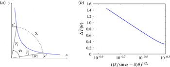
Sketch of the system of coordinates used for the asymptotic analysis of the residence time close to the stagnation point (a) and semi-logarithmic plot of the residence time as a function of the angle at the inlet (b) for
 ${\it\alpha}={\rm\pi}/3$
. As
 ${\it\theta}\rightarrow 0$
the residence time diverges logarithmically.

where
 ${\it\epsilon}^{\prime }$
is the distance to the
 $x$
and
 $y$
axes. The residence time is therefore
 $$\begin{eqnarray}\displaystyle {\rm\Delta}\tilde{T}({\it\varphi}) & = & \displaystyle -\frac{1}{2{\it\gamma}}\displaystyle \int _{\tilde{r}_{1}^{\prime }}^{\tilde{r}_{2}^{\prime }}\frac{\text{d}\tilde{r}^{\prime }}{\tilde{r}^{\prime }}=-\frac{1}{2{\it\gamma}}\left(\log \left(\frac{{\it\epsilon}^{\prime }}{\sin {\it\varphi}}\right)-\log \left(\frac{{\it\epsilon}^{\prime }}{\cos {\it\varphi}}\right)\right)\end{eqnarray}$$
 $$\begin{eqnarray}\displaystyle & = & \displaystyle \frac{1}{2{\it\gamma}}\log (\tan {\it\varphi}).\end{eqnarray}$$
The angle
 ${\it\varphi}$
and the angle at the inlet
 ${\it\theta}$
are linked by
 $$\begin{eqnarray}{\it\varphi}=\frac{{\rm\pi}}{2}-\arctan \left(\frac{{\it\delta}\sin {\it\theta}}{\sin {\it\alpha}-{\it\delta}\cos {\it\theta}}\right),\end{eqnarray}$$
where
 ${\it\delta}$
was taken to be strictly positive. The residence time can now be expressed as a function of
 ${\it\theta}$
; (3.23) becomes
 $$\begin{eqnarray}{\rm\Delta}\tilde{T}({\it\theta})=\frac{1}{2{\it\gamma}}\log \left(\frac{\sin {\it\alpha}-{\it\delta}\cos {\it\theta}}{{\it\delta}\sin {\it\theta}}\right).\end{eqnarray}$$
As the streamlines get closer to the stagnation point
 ${\it\theta}\rightarrow 0$
, and
 ${\rm\Delta}\tilde{T}$
is expressed as
 $$\begin{eqnarray}{\rm\Delta}\tilde{T}({\it\theta})=\frac{1}{2{\it\gamma}}\log \left(\frac{\sin {\it\alpha}}{{\it\delta}}-1\right)-\frac{1}{2{\it\gamma}}\log {\it\theta}-\frac{2{\it\delta}+\sin {\it\alpha}}{12{\it\gamma}({\it\delta}-\sin {\it\alpha})}{\it\theta}^{2}+O({\it\theta}^{3}).\end{eqnarray}$$
The singularity in residence time at the stagnation streamline is to the first order logarithmic in
 ${\it\theta}$
(see figure 7
b), and its amplitude is dependent on
 ${\it\alpha}$
and
 ${\it\delta}$
. The average residence time for
 $-{\it\xi}\leqslant {\it\theta}\leqslant {\it\xi}$
, where
 $0<{\it\xi}\ll 1$
, satisfies
 $$\begin{eqnarray}\langle \tilde{T}\rangle =\frac{1}{2{\it\omega}}\int _{-{\it\xi}}^{{\it\xi}}{\rm\Delta}\tilde{T}({\it\theta})\,\text{d}{\it\theta}\sim \frac{{\it\xi}}{2{\it\gamma}{\it\omega}}\log \left(\frac{\sin {\it\alpha}}{{\it\delta}}-1\right)-\frac{1}{4{\it\gamma}{\it\omega}}\int _{-{\it\xi}}^{{\it\xi}}\log |{\it\theta}|\,\text{d}{\it\theta}.\end{eqnarray}$$
The limit of the first term as
 ${\it\xi}\rightarrow 0$
is zero. Since
 $$\begin{eqnarray}\int _{-{\it\xi}}^{{\it\xi}}\log |{\it\theta}|\,\text{d}{\it\theta}=2{\it\xi}(\log {\it\xi}-1),\end{eqnarray}$$
the limit of the integral as
 ${\it\xi}\rightarrow 0$
is also zero. As a result, the singularity in residence time is integrable, and the average residence time is finite.
The impact of the heterogeneity in the residence time distribution on the bulk flow can be observed in figure 8, which shows the evolution of
 ${\rm\Delta}\tilde{p}$
,
 $\langle \tilde{T}\rangle$
and
 $\langle \tilde{T}\rangle _{RMS}$
with
 ${\it\omega}$
. The dispersion of the residence time distribution is introduced by the stagnation point, therefore
 $\langle \tilde{T}\rangle _{RMS}$
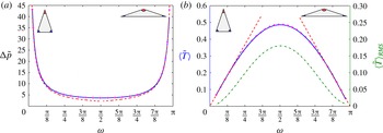
is a measure of the relative impact of the stagnation point on the bulk flow. The maximum in average residence time coincides with the minimum in pressure drop and with the maximum in
 $\langle \tilde{T}\rangle _{RMS}$
, obtained for
 ${\it\omega}={\rm\pi}/2$
(see § 4.3 for analytical proof). As
 $|{\rm\pi}/2-{\it\omega}|$
decreases, the impact of the stagnation point on the bulk flow increases. The next section describes the behaviour of
 ${\rm\Delta}\tilde{p}$
and
 $\langle \tilde{T}\rangle$
for small and large angles at the inlet.
Evolution of (a) the pressure drop and (b) the residence time and root of the mean square of the residence time (dash-dotted line) with the angle at the inlet
 ${\it\omega}$
calculated analytically by conformal mapping (solid line) and numerically using the FEM method (
 $+$
). The asymptotic expressions (3.32)–(3.34) are plotted as dashed lines. The minimum value of the pressure drop and the maximal value for the average residence time are obtained for
 ${\it\omega}={\rm\pi}/2$
.

3.3. Asymptotic approximation for narrow domains
For
 $|{\it\omega}|\ll 1$
and
 $|{\rm\pi}-{\it\omega}|\ll 1$
, the stagnation point has a weak impact on the global flow, and the residence time distribution is close to a uniform distribution. An asymptotic approximation for
 ${\rm\Delta}\tilde{p}$
and
 $\langle \tilde{T}\rangle$
can be calculated by approximating the pressure potential within
 ${\it\Omega}$
by the potential created by a source located at a unit distance from an outlet. The flow is dominated by a source flow, so that the radial velocity is approximately
 $$\begin{eqnarray}\tilde{u} _{r}\simeq \frac{1}{{\it\omega}\tilde{r}},\end{eqnarray}$$
where
 $\tilde{r}$
is the radial distance from the source, with
 ${\it\delta}\leqslant \tilde{r}\leqslant 1-{\it\delta}$
. Near the stagnation point this approximation is not valid since
 $|\tilde{\boldsymbol{u}}_{\boldsymbol{h}}|$
is greatly reduced and the residence time increases. Using (2.18) and the boundary condition
 $\tilde{p}=0$
at the outlet, the pressure potential is approximately
 $$\begin{eqnarray}\tilde{p}\simeq \frac{1}{{\it\omega}}\log \left(\frac{1-{\it\delta}}{\tilde{r}}\right),\end{eqnarray}$$
so that the pressure drop is expressed as
 $$\begin{eqnarray}{\rm\Delta}\tilde{p}\simeq \frac{1}{{\it\omega}}\log \frac{1-{\it\delta}}{{\it\delta}}.\end{eqnarray}$$
The residence time between the source and the outlet is
 $$\begin{eqnarray}{\rm\Delta}\tilde{T}\simeq \int _{{\it\delta}}^{1-{\it\delta}}\frac{\text{d}\tilde{r}}{\tilde{u} _{r}}=\frac{{\it\omega}}{2}((1-{\it\delta})^{2}-{\it\delta}^{2}),\end{eqnarray}$$
so that the average residence time is expressed as
 $$\begin{eqnarray}\langle \tilde{T}\rangle =\frac{1}{{\it\omega}}\int _{-{\it\omega}/2}^{{\it\omega}/2}{\rm\Delta}\tilde{T}\,\text{d}{\it\theta}\simeq \frac{{\it\omega}}{2}((1-{\it\delta})^{2}-{\it\delta}^{2}).\end{eqnarray}$$
When
 $|{\rm\pi}-{\it\omega}|\ll 1$
,
 $|{\it\alpha}|\ll 1$
, and the streamline pattern is similar to the case
 $|{\it\omega}|\ll 1$
, so that
 $$\begin{eqnarray}{\rm\Delta}\tilde{p}\simeq \frac{{\it\delta}}{2{\it\alpha}}\log \frac{1-{\it\delta}}{{\it\delta}},\quad \langle \tilde{T}\rangle \simeq {\it\alpha}((1-{\it\delta})^{2}-{\it\delta}^{2}).\end{eqnarray}$$
The asymptotic expressions for the dependence of the pressure drop and residence time for varying values of
 ${\it\omega}$
are plotted in figure 8(a,b). They give good predictions for small and wide angles at the source. Their accuracy decreases as the dispersion in residence time introduced by the stagnation point increases.
4. Influence of the void volume fraction on the pressure and residence time
The previous section described the dependence of the pressure drop and fluid residence time on the angle at the inlet
 ${\it\omega}$
. In this section, the effect of the void volume fraction
 ${\it\Phi}$
, which varies between 0.25 and 0.5 over the eye globe, is investigated numerically and analytically using Darwin’s (Reference Darwin1953) drift framework, which provides a means of quantifying fluid particle transport and dispersion within the bounded domain
 ${\it\Omega}$
. Initially considered within unbounded domains, Darwin’s (Reference Darwin1953) drift volume is defined as the fluid parcel, which keeps a constant mass, permanently displaced as a result of the progression of a material surface starting infinitely far from in front of a fixed body, and swept infinitely far past the body. This volume, denoted
 $D_{f}$
, satisfies
 $$\begin{eqnarray}D_{f}=\int _{A_{\infty }}X\,\text{d}A=C_{m}\mathscr{V},\end{eqnarray}$$
where
 $X$
is the fluid particle displacement,
 $\mathscr{V}$
is the body volume,
 $A_{\infty }$
spans the entire flow and
 $C_{m}$
is the added-mass coefficient;
 $C_{m}=1$
for a cylinder (Darwin Reference Darwin1953). Darwin’s (Reference Darwin1953) proposition was further investigated by Lighthill (Reference Lighthill1956), Yih (Reference Yih1985, Reference Yih1997), Benjamin (Reference Benjamin1986) and Eames, Belcher & Hunt (Reference Eames, Belcher and Hunt1994). If the flow is bounded, a return flow, or reflux, is also present. Eames, Hunt & Belcher (Reference Eames, Hunt and Belcher2004) showed that in a bounded rectangular channel, the fluid particle displacement field created by a distribution of fixed bodies placed in a uniform flow has two components: a local drift contribution
 $X_{d}$
close to the body, which decays rapidly away from the body, and a non-local reflux component
 $X_{r}$
, which decays slowly away from the body and depends on the far-field boundary conditions. Darwin’s (Reference Darwin1953) drift has to the best of our knowledge never been investigated in a diverging channel. The Darwin (Reference Darwin1953) drift framework is of interest here because the drift volume is a determinant of the longitudinal dispersivity induced by the cylinder array (Eames & Bush Reference Eames and Bush1999), and is therefore a measure of advective mixing. Furthermore, the average residence time
 $\langle \tilde{T}\rangle$
is related to the mean displacement
 $\bar{X}$
through (Lighthill Reference Lighthill1956)
 $$\begin{eqnarray}\langle \tilde{T}\rangle =\frac{1}{\bar{U}}+\frac{\bar{X}}{\bar{U}}.\end{eqnarray}$$
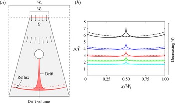
A schematic of the drift volume and reflux components in a diverging channel can be found in figure 9(a). Figure 9(b) shows the residence time, calculated numerically, for increasingly divergent channels and a single cylinder. The sharp increase in the residence time observed in the neighbourhood of
 $x/W_{i}=0$
is caused by the local drift contribution. As
 $|x/W_{i}|$
increases,
 $\langle \tilde{T}\rangle$
decreases below the value that it would take if the cylinder was absent (dashed lines). This is caused by the non-local reflux component. Figure 9(b) shows that as the divergence of the channel increases, the impact of both local and non-local reflux contributions on the residence time increases.
(a) Definition sketch of the drift volume in a diverging channel and (b) evolution of the residence time as a function of
 $x/W_{i}$
for decreasing values of
 $W_{i}$
. In (a), the dashed line corresponds to the flow profile in the absence of the cylinder. In (b), the dashed line corresponds to the residence time for the geometry described in (a) in the absence of the cylinder.

4.1. Numerical analysis
The pressure drop and the residence time were calculated over a range
 $0\leqslant {\it\Phi}\leqslant 0.62$
, where the upper limit is determined by the packing fraction. Once the maximal void fraction achievable was approximated through several simulations, random positions for the cylinders for the maximal void fraction were generated. The diameter of the cylinders was decrementally reduced to vary
 ${\it\Phi}$
.
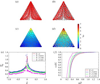
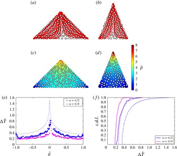
The cylinders have a local and a bulk effect on the pressure and residence time. A comparison between figures 5(c,d) and 11(c,d) and figure 10(c,d) shows that the cylinders lead to an overall increase in the pressure field. The pressure has a more homogeneous distribution over the triangles, with less abrupt variations. The fluid particle residence time decreases with
 ${\it\Phi}$
(figure 10
e,f). A stagnation point is located on the surface of each cylinder, which leads to a local divergence of the residence time (figures 10
e,f and 11
e,f). The missing values in the residence time distribution are due to the non-convergence of the streamline calculation for the fluid particles entering the vicinity of these stagnations points. They correspond to a local logarithmic divergence relative to the centre of the cylinder (Eames et al.
Reference Eames, Belcher and Hunt1994). The local singularities in the residence time are determined by the position of the cylinders. Therefore their distribution has an impact on the local behaviour of the residence time.
Streamlines of the flow (a,b), pressure field (c,d), residence time distribution (e) and c.d.f. ( f) for
 ${\it\omega}={\rm\pi}/3$
,
 ${\it\Phi}=0.13$
and
 ${\it\Phi}=0.3251$
. The residence time and c.d.f. for
 ${\it\Phi}=0$
and
 ${\it\Phi}=0.0332$
are also shown. The residence time was calculated for 1000 particles released at the inlet.

Streamlines of the flow (a,b), pressure field (c,d), residence time distribution (e) and c.d.f. (f) for (
 ${\it\omega}={\rm\pi}/2$
,
 ${\it\Phi}=0.2881$
) and (
 ${\it\omega}={\rm\pi}/4$
,
 ${\it\Phi}=0.2853$
). The dotted lines correspond to
 ${\rm\Delta}\tilde{T}$
and the c.d.f. when
 ${\it\Phi}=0$
. The residence time was calculated for 1000 particles released at the inlet.

Evolution of (a) the pressure drop
 ${\rm\Delta}\tilde{p}/{\rm\Delta}\tilde{p}({\it\Phi}=0)$
and (b) the residence time
 $\langle \tilde{T}\rangle /\langle \tilde{T}\rangle ({\it\Phi}=0)$
(calculated for 400 particles released at the inlet) with the void volume fraction
 ${\it\Phi}$
for a fixed distribution of cylinders for a range of
 ${\it\omega}$
. The approximate and analytical expressions obtained for
 ${\rm\Delta}\tilde{p}$
and
 $\langle \tilde{T}\rangle$
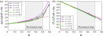
are plotted as dashed lines. The arrow under ‘Physiological range’ appears to be thicker in (a) than it is in (b).

The effect of the cylinders on the bulk flow is shown in figure 12. As
 ${\it\Phi}$
increases, the fraction of the fluid domain is reduced. As a result, the pressure drop increases (figure 12
a), and the bulk flow velocity increases, which leads to a decrease in the average residence time (figure 12
b). In the next section, an asymptotic expression for the evolution of
 ${\rm\Delta}\tilde{p}$
for small and wide angles at the inlet is sought.
4.2. Asymptotic analysis of the pressure drop for narrow domains
When
 $|{\it\omega}|\ll 1$
, the outlets are close and the stagnation point has a weak effect on the global flow. The flow within the triangles can be modelled as a diverging channel flow set by a uniform stream of velocity
 $\bar{U}$
at the inlet (see figure 9
a). The pressure is set to zero at the outlet. The case
 $|{\rm\pi}-{\it\omega}|\ll 1$
is symmetrical. The pressure drop can be calculated by considering the drop in velocity potential
 ${\it\phi}=-\tilde{p}$
between the inlet and the outlet of the diverging channel:
 $$\begin{eqnarray}{\rm\Delta}{\it\phi}=\frac{1}{\tilde{S}_{inlet}}\displaystyle \int _{\mathit{inlet}}^{}{\it\phi}\,\text{d}S=\frac{1}{\tilde{S}_{inlet}}\displaystyle \int _{\mathit{W}}^{}{\it\phi}n_{x}\,\text{d}S,\end{eqnarray}$$
where
 $W$
represents the boundaries of the diverging channel composed of the inlet, outlet and side walls. The second term in (4.3) can be calculated by considering the volume integral of
 $\boldsymbol{{\rm\nabla}}{\it\phi}$
over the volume of the channel deprived of the volume of the bodies. The volume integral can be decomposed as the sum of the contributions of the boundaries of the diverging channel
 $W$
and of the
 $N$
cylinders, labelled
 $i=1,2,\dots ,N$
,
 $$\begin{eqnarray}\displaystyle \int _{W}^{}{\it\phi}n_{x}\,\text{d}S=\displaystyle \int _{\mathscr{V}_{t}-\mathscr{V}_{c}}^{}\boldsymbol{{\rm\nabla}}{\it\phi}\,\text{d}V-\mathop{\sum }_{i=1}^{N}\displaystyle \int _{S_{i}}^{}{\it\phi}n_{x}\,\text{d}S_{i},\end{eqnarray}$$
where
 $\mathscr{V}_{t}$
is the volume of the channel,
 $\mathscr{V}_{c}$
is the total volume occupied by the cylinders and
 $S_{i}$
is the surface of the
 $i$
th body. The velocity near the body can be decomposed as a sum of the near-field and far-field contributions, i.e.
 $$\begin{eqnarray}{\it\phi}=\bar{U}_{L_{i}}(x-x_{i})+{\it\phi}_{i},\end{eqnarray}$$
where
 ${\it\phi}_{i}$
is the velocity potential created by the body and
 $\bar{U}_{L_{i}}$
is the mean velocity in the vicinity of the
 $i$
th body. Close to the cylinder, the far-field contribution of the velocity potential is
 $$\begin{eqnarray}\displaystyle \int _{S_{i}}^{}\bar{U}_{L_{i}}(x-x_{i})n_{x}\,\text{d}S_{i}=\bar{U}_{L_{i}}\mathscr{A}_{c},\end{eqnarray}$$
where
 $\mathscr{A}_{c}$
is the cross-section of the body. The near-field contribution
 ${\it\phi}_{i}$
includes the interaction between bodies, and is mathematically composed of an infinite number of dipoles within the body to satisfy the kinematic boundary condition (2.15). The associated dipole moment
 ${\it\mu}_{i}$
is determined by the added-mass tensor. Since the bodies are symmetrical about the mean flow, the far-field contribution is determined by the component of the dipole moment parallel to the mean flow,
 ${\it\mu}_{i}=-(1+C_{m})\mathscr{A}_{c}\bar{U}/2{\rm\pi}$
. The near-field contribution (Eames et al.
Reference Eames, Hunt and Belcher2004, appendix) is therefore
 $$\begin{eqnarray}\displaystyle \int _{S_{i}}^{}{\it\phi}_{i}n_{x}\,\text{d}S=\frac{1}{2}(1+C_{m})\mathscr{A}_{c}\bar{U}_{L_{i}}.\end{eqnarray}$$
Since
 $$\begin{eqnarray}\displaystyle \int _{\mathscr{V}_{t}-\mathscr{V}_{c}}^{}\boldsymbol{{\rm\nabla}}{\it\phi}\,\text{d}V=-\mathscr{A}_{t}\mathop{\sum }_{i=1}^{N}\bar{U}_{L_{i}},\end{eqnarray}$$
(4.4) becomes
 $$\begin{eqnarray}\displaystyle \int _{W}^{}{\it\phi}n_{x}\,\text{d}S=-\mathscr{A}_{t}\mathop{\sum }_{i=1}^{N}\bar{U}_{L_{i}}-\left(1+\frac{1}{2}(1+C_{m})\right)\mathscr{A}_{c}\mathop{\sum }_{i=1}^{N}\bar{U}_{L_{i}}.\end{eqnarray}$$
The mean velocity in the vicinity of the bodies is
 $\bar{U}_{L_{i}}=\bar{U}/N$
, so that (4.3) becomes
 $$\begin{eqnarray}{\rm\Delta}{\it\phi}=-\frac{\mathscr{A}_{t}\bar{U}}{\tilde{S}_{inlet}}\left(1+\left(1+\frac{1}{2}(1+C_{m})\right){\it\Phi}\right).\end{eqnarray}$$
Since
 ${\rm\Delta}{\it\phi}({\it\Phi}=0)=-\mathscr{A}_{t}\bar{U}/\tilde{S}_{inlet}$
, the pressure drop is
 $$\begin{eqnarray}\frac{{\rm\Delta}\tilde{p}}{{\rm\Delta}\tilde{p}({\it\Phi}=0)}=1+\frac{1}{2}(3+C_{m}){\it\Phi}.\end{eqnarray}$$
This shows that the average pressure drop in narrow domains depends on the shape of the avascular septae, which are characterised by the added-mass coefficient. The approximate expressions for the pressure drop are plotted in figure 12. As the void fraction increases the flow interactions between bodies cannot be neglected and the approximation stops being valid.
4.3. Analytical expression for the average residence time
The average residence time satisfies
 $$\begin{eqnarray}\langle \tilde{T}\rangle =\frac{1}{{\rm\Delta}{\it\psi}}\displaystyle \int _{{\it\psi}_{1}}^{{\it\psi}_{2}}{\rm\Delta}\tilde{T}\,\text{d}{\it\psi},\end{eqnarray}$$
where
 ${\rm\Delta}{\it\psi}={\it\psi}_{2}-{\it\psi}_{1}$
is the difference of the streamfunction
 ${\it\psi}$
over the inlet. As a result,
 $$\begin{eqnarray}\langle \tilde{T}\rangle =\frac{1}{{\rm\Delta}{\it\psi}}\displaystyle \int _{{\it\psi}_{1}}^{{\it\psi}_{2}}\displaystyle \int _{{\it\psi}_{\tilde{S}}}^{}\frac{1}{|\tilde{\boldsymbol{u}}_{h}|}\,\text{d}\tilde{s}\,\text{d}{\it\psi}=\frac{1}{{\rm\Delta}{\it\psi}}\displaystyle \int _{{\it\psi}_{1}}^{{\it\psi}_{2}}\displaystyle \int _{{\it\psi}_{\tilde{S}}}^{}\frac{1}{|\tilde{\boldsymbol{u}}_{h}|^{2}}\,\text{d}{\it\phi}\,\text{d}{\it\psi}=\frac{1}{{\rm\Delta}{\it\psi}}\displaystyle \int _{\mathscr{A}_{t}-\mathscr{A}_{c}}^{}\,\text{d}x\,\text{d}y.\end{eqnarray}$$
Since
 $$\begin{eqnarray}\displaystyle \int _{\mathscr{A}_{t}-\mathscr{A}_{c}}^{}\,\text{d}x\,\text{d}y=\mathscr{A}_{t}(1-{\it\Phi}),\end{eqnarray}$$
then
 $$\begin{eqnarray}\langle \tilde{T}\rangle =\frac{\mathscr{A}_{t}}{q}(1-{\it\Phi}),\end{eqnarray}$$
where
 $q={\rm\Delta}{\it\psi}$
is the area flux into the domain. This expression provides an analytical expression for
 $\langle \tilde{T}\rangle$
when
 ${\it\Phi}=0$
:
 $$\begin{eqnarray}\langle \tilde{T}\rangle ({\it\Phi}=0)=\left(\frac{\sin {\it\omega}}{2}-\frac{{\rm\pi}{\it\delta}^{2}}{2}\right).\end{eqnarray}$$
The residence time of the geometry deprived of the bodies is a function of the area of the flow domain and the area flux into the domain. This expression shows that the average residence time is maximum for
 ${\it\omega}={\rm\pi}/2$
, and is obtained when
 $\langle \tilde{T}\rangle _{RMS}$
is maximal (see figure 8
b). In the case where
 $|{\it\omega}|\ll 1$
, a first-order expansion of (4.16) yields
 $$\begin{eqnarray}\langle \tilde{T}\rangle ({\it\Phi}=0)=\frac{{\it\omega}}{2}\left(1-\frac{{\rm\pi}{\it\delta}^{2}}{{\it\omega}}\right)+O({\it\omega}^{3})=\frac{{\it\omega}}{2}\left(1-\frac{{\it\delta}^{2}}{\displaystyle 1-\frac{2{\it\alpha}}{{\rm\pi}}}\right)+O({\it\omega}^{3}).\end{eqnarray}$$
Since
 $|{\it\omega}|\ll 1$
,
 $|1-2{\it\alpha}/{\rm\pi}|\ll 1$
. An expansion to the first order brings
 $$\begin{eqnarray}\langle \tilde{T}\rangle ({\it\Phi}=0)=\frac{{\it\omega}}{2}(1-{\it\delta}^{2})+O({\it\omega}^{3}).\end{eqnarray}$$
For
 ${\it\delta}$
small,
 $|(1-{\it\delta})^{2}-1|\ll 1$
, so that to the first order expression (4.18) coincides with the asymptotic expression (3.33). Expression (3.34) can be obtained through a similar approach.
Equation (4.15) yields
 $$\begin{eqnarray}\frac{\langle \tilde{T}\rangle }{\langle \tilde{T}\rangle ({\it\Phi}=0)}=1-{\it\Phi}.\end{eqnarray}$$
This shows that the average residence time is independent of the mass coefficient
 $C_{m}$
, and is therefore independent of the shape of the avascular septae. It is dependent on their cross-sectional area, which blocks the flow and increases the average speed. No assumptions were made on
 ${\it\Phi}$
, so that (4.19) does not depend on
 ${\it\Phi}$
being small. This result is a generalisation of the relation obtained by Eames et al. (Reference Eames, Hunt and Belcher2004) for rectangular bounded flows.
Equation (4.19) gives a good fit for all values of
 ${\it\omega}$
and
 ${\it\Phi}$
(see figure 12
b). The divergence of
 $\langle \tilde{T}\rangle /\langle \tilde{T}\rangle ({\it\Phi}=0)$
from expression (4.19) is due to an increase in the number of failed streamline calculations with
 ${\it\Phi}$
. This is caused by the reduction of the space between cylinders as their diameter increases. For
 ${\it\Phi}$
approaching the packing fraction (which is a function of the area of the triangle), portions of the triangle become constricted. For
 $|{\it\omega}|\ll 1$
and
 $|{\rm\pi}-{\it\omega}|\ll 1$
, constriction occurs for smaller values of
 ${\it\Phi}$
, and results in the closure of significant portions of the flow domain.
5. Discussion and conclusion
This paper describes the first theoretical model for the blood flow and corpuscle transport in the choriocapillaris, a vascular bed located in the back of the eye and responsible for the metabolite supply to the photoreceptors. The model is based on direct observations of the human choriocapillaris and on an extensive literature search. It describes the flow within the boundaries of an elementary vascular unit reduced to a triangular portion. The choriocapillaris is composed of a juxtaposition of independent lobules of various shapes. Within each of these lobules the blood flow is largely passive, set by the pressure drop between feeding arterioles and draining venules and directed by avascular septae. This theoretical analysis sheds light on the interdependence of the pressure drop, the fluid residence time, the angle at the inlet and the void volume fraction. An analytical resolution of the equations for the flow was developed in the limit where the void fraction is small. The impact of the cylinders on the flow was characterised using a numerical study and a drift analysis.
This model represents an idealisation of the physiology of the capillary bed, and as such presents some limitations. Despite being justified by the high vascular fraction of the capillaries, the continuum approach deprives this analysis of some aspects of the interactions between blood and capillary vessel wall. Movements from the blood vessels to the tissue such as filtration and reabsorption were not modelled. Another important limitation pertains to the two-dimensional analysis of the residence time. The fluid residence time analysed here only provides a metric of the transport of corpuscles in a choriocapillaris lobule. The travel time and distribution of weakly diffusive tracer species depend critically on the three-dimensionality of the flow and the recirculating regions in the vicinity of the cylinders, which are a consequence of the low Reynolds number. Moreover, the cylinders represent a boundary between vasculature and tissue, and may as such involve diffusion across their surfaces. To alleviate these limitations, the full advection–diffusion equations need to be considered to fully describe the passive transport of solutes.
Despite these limitations, the approach described in this paper constitutes a first step towards understanding better the biology and physiology of the choriocapillaris and the metabolite delivery system to the photoreceptors. A strength of the model is that it is flexible enough to incorporate spatial variations in the choriocapillaris anatomy and physiology, and therefore to present possible functional explanations for some aspects of the morphology of this capillary bed.
Based on our assumptions, this analysis suggests that the pressure drop and residence time between inlets and outlets are set by the topology of the flow domain. Close to the triangle walls, the flow is a quasi-parallel flow characterised by a shorter and quasi-uniform residence time. The flow close to the stagnation point is characterised by a longer path and a prolonged residence time, diverging logarithmically with the distance to the stagnation streamline. The angle at the inlet sets the relative importance of each component on the pressure drop and average residence time. Although the choriocapillaris lacks autoregulation, evidence suggests that the blood flow within the arteries servicing it is vasoregulated (Condren et al.
Reference Condren, Kumar, Mettu, Liang, Zhao, Yue Tsai, Fariss and Wong2013). The mural cells involved in this regulation decrease in number and density as the primary arteries branch out and travel parallel to the plane of the choriocapillaris, which may result in a decreased regulation. Regardless of this regulation, our analysis shows that the blood pressure drop can be modulated by modifying the angle
 ${\it\omega}$
between arterioles and venules. This may explain the local variations in
 ${\it\omega}$
described in table 1.
The avascular septae have two effects on the flow. As a result of the reduction of the flow domain, the bulk flow velocity is increased, which results in a decrease of the average residence time. The septae also lead to a local increase in the residence time due to the stagnation region at the separation point of the streamlines on their surface. The analysis carried out within Darwin’s (Reference Darwin1953) drift framework led to the formulation of exact and approximate expressions for the pressure drop and average residence time. The pressure drop has a dependence on the shape of the septae, and increases quasi-linearly with the void fraction. The average residence time is independent of the shape of the septae, and decreases linearly with the void fraction. Our model suggests that the spatial variations in the void fraction over the eye globe may be a way of locally tuning the pressure drop and average blood travel time in lobules.
A major consequence of the topology of the choriocapillaris is the non-uniformity of the blood velocity and residence time over choriocapillaris lobules. This finding is supported by the results from Zhu et al. (Reference Zhu, Zheng, von Kerczek, Topoleski and Flower2006), who observed that the blood velocity in the choriocapillaris varied locally between 0.5 and
 $2.5~\text{mm}~\text{s}^{-1}$
. The heterogeneity in fluid residence time in the choriocapillaris has to the best of our knowledge never been emphasised. The heterogeneities described in this model could be partly responsible for the strong geographical variation in susceptibility observed in some eye pathologies such as AMD. In one of its forms, AMD is characterised by the accumulation of deposits called drusen in what appear to be singular regions of the eye. Friedman, Smith & Kuwabara (Reference Friedman, Smith and Kuwabara1963) suggested that there is a relationship between the location of drusen and the choriocapillaris. They also observed that drusen tend to appear close to venular openings, which in our model correspond to the regions with the longest residence time. This relationship has not been further explored quantitatively.
As a novel way of describing the linkage between choriocapillaris structure and function, this model may help in giving directions to the biological and clinical communities in the collection of anatomical and physiological data. At present, measurements are sparse and often inconsistent. Some of the parameters that were found to be critical in our analysis, such as
 ${\it\omega}$
, have simply never been investigated by anatomists or physiologists. While several in vivo measurements of the blood flow velocity in the human choriocapillaris are available in the literature and show a satisfying level of consistency, only one value for the pressure drop between an arteriolar and a venular opening was found (see table 1). The value was measured in the rabbit eye using a highly invasive micropuncture method, which was likely to have a non-negligible impact on the pressure balance within the circulation. Furthermore, the measurements were taken blindly over extended regions of the choriocapillaris (Mäepa Reference Mäepa1992). Using the commonly accepted value for the blood velocity in the human choriocapillaris and the pressure drop from Mäepa (Reference Mäepa1992), the choriocapillaris permeability is of the order of
 ${\it\mu}\mathscr{Q}_{a}/h{\rm\Delta}p\sim 10^{-14}~\text{m}^{2}$
. This value is much smaller than the one obtained with the parallel-plate approximation,
 $K=h^{2}/12\sim 10^{-11}~\text{m}^{2}$
. However, because of a lack of consistency in the data, its validity is questionable.
Our future work will focus on strengthening this approach by investigating the mass transport within lobules, and the mass exchanges between the choriocapillaris and the outer retina, using the three-dimensional solution of the Navier–Stokes and advection–diffusion equations.
Acknowledgements
The authors gratefully acknowledge the support from the Special Trustees of Moorfields Eye Hospital, London, the National Institute for Health Research (NIHR) Biomedical Research Centre at Moorfields Eye Hospital NHS Foundation Trust and UCL Institute of Ophthalmology, London and the University College London Impact Studentship Scheme.