1 Introduction
Quantum effects in plasmas have been addressed since at least the mid-1900s (Bohm & Pines Reference Bohm and Pines1950; Silin Reference Silin1958; Pines Reference Pines1961), and have also been a subject of renewed interest recently (Marklund et al. Reference Marklund, Brodin, Stenflo and Liu2008; Shukla & Eliasson Reference Shukla and Eliasson2011; Tyshetskiy, Vladimirov & Kompaneets Reference Tyshetskiy, Vladimirov and Kompaneets2011; Vladimirov & Tyshetskiy Reference Vladimirov and Tyshetskiy2011). The reason for this renewed interest is twofold: it is due to the increasing importance of plasma effects in certain quantum solid-state systems (Marklund et al. Reference Marklund, Brodin, Stenflo and Liu2008) on the one hand, and the increasing importance of quantum effects in dense plasmas in the laboratory (Glenzer et al. Reference Glenzer, Landen, Neumayer, Lee, Widmann, Pollaine, Wallace, Gregori, Höll and Bornath2007) and in astrophysics (Chabrier, Douchin & Potekhin Reference Chabrier, Douchin and Potekhin2002) on the other hand. As quantum effects generally occur at small scales, it is reasonable to first apply quantum mechanics to problems in kinetic plasma theory. Important topics which require kinetic physics include transport theory and the linear modes and stability properties of a plasma. This paper is concerned with the latter. Linear physics is also important because linear problems can often be solved analytically and are amenable to simple interpretation. For this reason, much of our understanding of complex processes in classical plasmas is founded upon knowledge of the linear properties, and it can be expected that this will hold true for quantum plasmas as well. Additionally, the comparative simplicity of non-relativistic quantum plasma physics serves as a useful baseline for more difficult problems in quantum plasma physics, such as relativistic quantum-electrodynamic (QED) plasmas with significance to fundamental theoretical physics and important astrophysical applications. It is therefore advantageous to understand the linear kinetic physics of non-relativistic quantum plasma waves.
The theory of linear waves in quantum plasmas has been studied alongside classical theory during the early development of plasma physics (Bohm & Pines Reference Bohm and Pines1950, Reference Bohm and Pines1953; Pines Reference Pines1961; Pines & Schrieffer Reference Pines and Schrieffer1962), as well as in more recent works (Bonitz et al. Reference Bonitz, Binder, Scott, Koch and Kremp1993, Reference Bonitz, Binder, Scott, Koch and Kremp1994; Haas, Manfredi & Goedert Reference Haas, Manfredi and Goedert2001; Haas, Bret & Shukla Reference Haas, Bret and Shukla2009; Eliasson & Shukla Reference Eliasson and Shukla2010; Melrose & Mushtaq Reference Melrose and Mushtaq2010a ). Studies of one-dimensional electrostatic waves in quantum plasmas have demonstrated unique effects due to quantum mechanics, including dependence of Landau damping rates on quantum effects (Krivitskii & Vladimirov Reference Krivitskii and Vladimirov1991; Melrose & Mushtaq Reference Melrose and Mushtaq2010a ; Rightley & Uzdensky Reference Rightley and Uzdensky2016) and the existence of entirely new modes that do not appear in classical plasmas (Krivitskii & Vladimirov Reference Krivitskii and Vladimirov1991). The introduction of a second, drifting population of particles broadens the parameter space by introducing a new density and temperature, and the separation velocity between the two populations. In classical plasmas, this introduces the possibility for growing unstable modes such as the Buneman, bump-on-tail, and ion-acoustic instabilities (Stix Reference Stix1992). The quantum counterparts of these streaming instabilities have been subject to a few isolated studies in the past decades, although so far no comprehensive systematic approach has yet been applied to kinetic quantum plasma instabilities. For instance, instabilities in one-dimensional quantum wires have been investigated by Bonitz et al. (Reference Bonitz, Binder, Scott, Koch and Kremp1993, Reference Bonitz, Binder, Scott, Koch and Kremp1994). Additionally, the Nyquist method has been applied to two-population quantum plasmas, and it has been demonstrated that a Penrose criterion does not exist for a quantum plasma (Haas et al. Reference Haas, Manfredi and Goedert2001). Thus, no general rule has been developed to show whether or not a two-population quantum plasma will be unstable. Furthermore, the existence of a second region of instability for sufficiently strong quantum effects has been demonstrated for a two-stream plasma by Haas et al. (Reference Haas, Bret and Shukla2009). Despite these interesting results, so far there has been no comprehensive mapping of the different instability types in quantum plasmas, in contrast to classical plasmas as discussed, for example, by Lapuerta & Ahedo (Reference Lapuerta and Ahedo2002). This is due in part to the difficulty of working with the Fermi–Dirac distribution function in the quantum kinetic theory, as noted by Krivitskii & Vladimirov (Reference Krivitskii and Vladimirov1991) and by Vladimirov & Tyshetskiy (Reference Vladimirov and Tyshetskiy2011).
The purpose of this paper is to explore quantum dynamical effects on linear electrostatic perturbations without the complexity of quantum statistics by utilising a number of simplified, analytically convenient distribution functions. We study a sequence of increasingly complex distribution functions in one- and two-population classical and quantum unmagnetised plasmas in order to look for regularities which may guide further study of more realistic Fermi–Dirac plasmas. We analyse the effects of quantum mechanics on the behaviour of linear perturbations in single-population plasmas and in plasmas consisting of two populations of electrons drifting relative to each other with a stationary neutralising ion background. After briefly describing the foundations of quantum kinetic theory in § 2, we examine the dispersion relation of waves in plasmas consisting of one electron population using several toy equilibrium Wigner distribution functions which allow the susceptibility to be integrated exactly (§ 3). Then, we consider potentially unstable plasmas with two electron populations in § 4. For each toy Wigner function we examine two cases: (i) the case of identical counter-drifting populations and (ii) the case of a main population with a zero-width drifting beam. We analyse and plot the dispersion relations, map the wavelengths and drift velocities that allow instabilities for different parameters of the distribution functions, and additionally map the growth rates and wavelengths of the fastest-growing modes. Each case is compared to the similar situation in a classical plasma in order to elucidate the differences due to quantum mechanics. Section 5 concerns the limitations and possible applications and extensions of this work. Finally, we draw conclusions as to the general effects of the shape of the Wigner function and of quantum recoil on streaming instabilities in § 6.
2 Formalism of non-relativistic quantum plasma physics
In this section a quantum kinetic theory based on Wigner functions is briefly reviewed in § 2.1. We then write down and discuss the longitudinal susceptibility for an unmagnetised collisionless plasma of arbitrary composition including the influence of quantum recoil and tunnelling in § 2.2. Subsequently, in § 2.3 we proceed to discuss the characteristic scales and important parameters of the system, and finally non-dimensionalise the susceptibility in preparation for the analysis that follows in § 3.
2.1 Quantum kinetic theory
In quantum mechanics, the state of a many-body system of particles may be described by its density operator
 $\hat{\unicode[STIX]{x1D70C}}$
. The time evolution of this operator under the influence of Hamiltonian
 ${\hat{H}}$
in the Heisenberg formalism is given by
 $\text{i}\hbar \unicode[STIX]{x2202}\hat{\unicode[STIX]{x1D70C}}/\unicode[STIX]{x2202}t=[{\hat{H}},\hat{\unicode[STIX]{x1D70C}}]$
.
This operator theory may be cast in an equivalent theory of functions in phase space
 $(\boldsymbol{x},\boldsymbol{p})$
by introducing the Wigner transformation
 $$\begin{eqnarray}\displaystyle W[\hat{A}]\equiv \int \text{d}^{3}\boldsymbol{y}\exp (-2\text{i}\boldsymbol{p}\boldsymbol{\cdot }\boldsymbol{y}/\hbar )\langle \boldsymbol{x}+\boldsymbol{y}|\hat{A}|\boldsymbol{x}-\boldsymbol{y}\rangle . & & \displaystyle\end{eqnarray}$$
The Wigner transformation of the density operator is the Wigner quasi-probability distribution function (Wigner Reference Wigner1932),
 $$\begin{eqnarray}\displaystyle f(\boldsymbol{x},\boldsymbol{p})\equiv W[\hat{\unicode[STIX]{x1D70C}}] & & \displaystyle\end{eqnarray}$$
and the Wigner transformation of the equation of motion of the density operator is the Moyal equation (Moyal Reference Moyal1949)
 $$\begin{eqnarray}\displaystyle \frac{\unicode[STIX]{x2202}f}{\unicode[STIX]{x2202}t}=-\frac{2}{\hbar }\left\{f(\boldsymbol{x},\boldsymbol{p})\sin \left[\frac{\hbar }{2}(\overleftarrow{\unicode[STIX]{x2202}_{\boldsymbol{x}}}\overrightarrow{\unicode[STIX]{x2202}_{\boldsymbol{p}}}-\overleftarrow{\unicode[STIX]{x2202}_{\boldsymbol{p}}}\overrightarrow{\unicode[STIX]{x2202}_{\boldsymbol{x}}})\right]H(\boldsymbol{x},\boldsymbol{p})\right\}, & & \displaystyle\end{eqnarray}$$
where the subscripts on the
 $\unicode[STIX]{x2202}$
operators indicate the relevant variable of differentiation, the arrows above the
 $\unicode[STIX]{x2202}$
operators indicate the function upon which they operate (
 $f$
on the left and
 $H$
on the right), and the
 $\sin$
function with operator argument is to be understood in terms of its Taylor expansion. The Wigner function plays the role of the classical distribution function in that its moments result in measurables such as the particle density, velocity and current. The Moyal equation thus plays the role of the Liouville equation and for a 1-particle Wigner function it plays the role of the Vlasov equation. Details of this theory have been reviewed by Liboff (Reference Liboff2003).
2.2 The quantum plasma longitudinal susceptibility
For easy comparison to wave phase velocities, we work in the
 $(\boldsymbol{x},\boldsymbol{v})$
phase space, where momentum is replaced with velocity through
 $\boldsymbol{v}=\boldsymbol{p}/m$
. The longitudinal susceptibility for a population
 $s$
drifting at velocity
 $\boldsymbol{U}_{s}$
with respect to a given reference frame in an unmagnetised plasma (Lindhard Reference Lindhard1954; Klimontovich & Silin Reference Klimontovich and Silin1960) is
 $$\begin{eqnarray}\displaystyle \unicode[STIX]{x1D712}_{s}(\unicode[STIX]{x1D714},\boldsymbol{k})=\frac{m_{s}\unicode[STIX]{x1D714}_{ps}^{2}}{2\hbar k^{2}}\int \text{d}^{3}\boldsymbol{v}\frac{F_{0s}(\boldsymbol{v}+\hbar \boldsymbol{k}/m_{s}-\boldsymbol{U}_{\boldsymbol{s}})-F_{0s}(\boldsymbol{v}-\hbar \boldsymbol{k}/m_{s}-\boldsymbol{U}_{\boldsymbol{s}})}{\unicode[STIX]{x1D714}-\boldsymbol{k}\boldsymbol{\cdot }\boldsymbol{v}}, & & \displaystyle\end{eqnarray}$$
where
 $F_{0s}(\boldsymbol{v})$
is the normalised background Wigner quasi-probability distribution function for species
 $s$
,
 $\unicode[STIX]{x1D714}_{ps}\equiv (4\unicode[STIX]{x03C0}n_{s}e^{2}/m_{s})^{1/2}$
is the population-specific plasma frequency.
For simplicity, we will assume modes parallel to
 $\boldsymbol{U}_{s}\boldsymbol{ : }\boldsymbol{k}\Vert \boldsymbol{U}_{s}$
. Modes propagating at angle
 $\unicode[STIX]{x1D703}$
with respect to
 $\boldsymbol{U}$
can be accounted for through the substitution
 $U\rightarrow U\cos \unicode[STIX]{x1D703}$
and a variable substitution in the integration over velocities perpendicular to
 $\boldsymbol{k}$
. For
 $\boldsymbol{k}\Vert \boldsymbol{U}_{s}$
, performing the integral over directions perpendicular to
 $\boldsymbol{k}$
and re-labelling
 $v$
as the parallel velocity component, one obtains
 $$\begin{eqnarray}\displaystyle \unicode[STIX]{x1D712}_{s}(\unicode[STIX]{x1D714},k)=\frac{m_{s}\unicode[STIX]{x1D714}_{ps}^{2}}{2\hbar k^{3}}\int _{C}\text{d}v\,\frac{f_{0s}(v+\hbar k/m_{s}-U_{s})-f_{0s}(v-\hbar k/m_{s}-U_{s})}{\unicode[STIX]{x1D714}/k-v}, & & \displaystyle\end{eqnarray}$$
where
 $f_{0s}(v)$
is now the reduced distribution function
 $$\begin{eqnarray}\displaystyle f_{0s}(v)=\int \text{d}^{2}v_{\bot }F_{0s}(\boldsymbol{v}), & & \displaystyle\end{eqnarray}$$
which is normalised to unity. The integral is performed along contour along the real-
 $v$
axis so as to pass below the pole at
 $v=\unicode[STIX]{x1D714}/k$
.
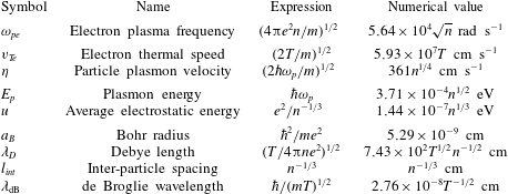
Table of relevant scales, with
 $T$
measured in eV and
 $n$
measured in
 $\text{cm}^{-3}$
.

For a multi-component plasma, we define the total plasma frequency
 $$\begin{eqnarray}\displaystyle \unicode[STIX]{x1D714}_{p}^{2}\equiv \mathop{\sum }_{s}\unicode[STIX]{x1D714}_{ps}^{2}=4\unicode[STIX]{x03C0}e^{2}n\mathop{\sum }_{s}\frac{{\tilde{n}}_{s}}{m_{s}}, & & \displaystyle\end{eqnarray}$$
where we have defined
 $$\begin{eqnarray}\displaystyle {\tilde{n}}_{s}\equiv \frac{n_{s}}{n}, & & \displaystyle\end{eqnarray}$$
to be the fraction of total particles in population
 $s$
, where
 $n$
is the total number density and
 $\sum _{s}{\tilde{n}}_{s}=1$
. At this point we assume that only electrons are mobile and that the ions form only a stationary neutralising background so that we can write
 $$\begin{eqnarray}\displaystyle m_{s}=m_{e}\equiv m. & & \displaystyle\end{eqnarray}$$
We then rewrite the susceptibility as
 $\unicode[STIX]{x1D712}_{s}={\tilde{n}}_{s}\tilde{\unicode[STIX]{x1D712}}_{s}$
where
 $$\begin{eqnarray}\displaystyle \tilde{\unicode[STIX]{x1D712}}_{s}(\unicode[STIX]{x1D714},k)=\frac{m\unicode[STIX]{x1D714}_{p}^{2}}{2\hbar k^{3}}\int _{-\infty }^{\infty }\text{d}v\frac{f_{0s}(v+\hbar k/m_{s}-U_{s})-f_{0s}(v-\hbar k/m_{s}-U_{s})}{\unicode[STIX]{x1D714}/k-v} & & \displaystyle\end{eqnarray}$$
is the susceptibility normalised to the total density. We then obtain the dispersion relation by solving the equation
 $$\begin{eqnarray}\displaystyle \unicode[STIX]{x1D716}(\unicode[STIX]{x1D714},k)\equiv 1+\mathop{\sum }_{s}\unicode[STIX]{x1D712}_{s}=0, & & \displaystyle\end{eqnarray}$$
where
 $\unicode[STIX]{x1D716}$
is the dielectric function, and write solutions of this equation as
 $\unicode[STIX]{x1D714}=\unicode[STIX]{x1D714}_{r}+\text{i}\unicode[STIX]{x1D6FE}$
.
2.3 Comments on parameters and scales
Before considering solutions of (2.11), we discuss the important scales involved in this study, the relevant parameter regimes, and the issue of non-dimensionalising the arguments and parameters of the dielectric function. The fundamental parameters that describe a one-component unmagnetised plasma are the total density
 $n$
and temperature
 $T$
. The density defines a length scale: the inter-particle spacing
 $n^{-1/3}$
, and the temperature determines the characteristic particle velocity
 ${\mathcal{V}}=(2T/m)^{1/2}$
. In addition the density determines the plasma frequency
 $\unicode[STIX]{x1D714}_{p}=(4\unicode[STIX]{x03C0}ne^{2}/m)^{1/2}$
, which in turn determines the plasmon energy
 $\unicode[STIX]{x1D716}_{p}=\hbar \unicode[STIX]{x1D714}_{p}$
. Another important velocity scale is the velocity of a particle with energy equal to the plasmon energy
 $\unicode[STIX]{x1D702}=(2\hbar \unicode[STIX]{x1D714}_{p}/m)^{1/2}$
, and an additional energy scale is the average electrostatic interaction energy
 $u=e^{2}/n^{-1/3}$
. Two final length scales that may be defined are the thermal de Broglie wavelength of the particles
 $\unicode[STIX]{x1D706}_{\text{dB}}=\hbar /(8\unicode[STIX]{x03C0}^{2}mT)^{1/2}$
and the Debye length
 $\unicode[STIX]{x1D706}_{D}={\mathcal{V}}/\unicode[STIX]{x1D714}_{p}=(T/4\unicode[STIX]{x03C0}ne^{2})^{1/2}$
. For Fermi–Dirac electrons, there additionally exists the Fermi energy
 $E_{F}=\hbar ^{2}(3\unicode[STIX]{x03C0}n)^{2/3}/2m$
and, as the characteristic velocity depends on the level of degeneracy, we define degeneracy-dependent speed and screening length
 $V_{\ast }$
and
 $\unicode[STIX]{x1D706}_{\ast }$
respectively, as in Rightley & Uzdensky (Reference Rightley and Uzdensky2016). These characteristic scales are summarised in table 1. From these scales we can define a number of dimensionless parameters, the values of which determine the relative importance of different processes in the plasma. Length scales can be compared to the inter-particle spacing by examining the number of particles in a cubic volume bounded by the relevant length:
 $\unicode[STIX]{x1D6E4}\equiv n\unicode[STIX]{x1D706}_{D}^{3}$
, which is the classical plasma parameter describing the relative importance of electrostatic interactions and
 $\unicode[STIX]{x1D6E9}\equiv n\unicode[STIX]{x1D706}_{\text{dB}}^{3}\propto (T/E_{F})^{-3/2}$
, which is a proxy for the level of degeneracy. We can also consider the ratio
 $\unicode[STIX]{x1D706}_{\text{dB}}/\unicode[STIX]{x1D706}_{D}$
which determines the relative importance of quantum effects for wave phenomena. We further create three dimensionless numbers using the three energy scales:
 $H\equiv \unicode[STIX]{x1D706}_{\text{dB}}/\unicode[STIX]{x1D706}_{\ast }=\hbar \unicode[STIX]{x1D714}_{p}/4\unicode[STIX]{x03C0}T$
,
 $N_{B}\equiv a_{B}n^{1/3}=(\hbar \unicode[STIX]{x1D714}_{p}/u)^{2}/4\unicode[STIX]{x03C0}$
and
 $u/T\propto \unicode[STIX]{x1D6E4}^{-2/3}$
. These dimensionless parameters are summarised in table 2.
It is computationally convenient to remove dimensions from the susceptibility. This task can be accomplished using two schemes. In both schemes a logical time scale is the plasma frequency
 $\unicode[STIX]{x1D714}_{p}$
. There are two ways, however, of introducing a velocity (and by proxy, length) scale: (i) use the characteristic particle velocity of the background distribution function
 ${\mathcal{V}}$
, and (ii) use the velocity
 $\unicode[STIX]{x1D702}$
, which is independent of the normalised distribution function. In scheme
 $1$
we introduce variables
 $\tilde{v}\equiv v/{\mathcal{V}}_{s}$
,
 $\unicode[STIX]{x1D6FA}\equiv \unicode[STIX]{x1D714}/\unicode[STIX]{x1D714}_{p}$
,
 $K\equiv k{\mathcal{V}}_{s}/\unicode[STIX]{x1D714}_{p}$
,
 $H\equiv \hbar \unicode[STIX]{x1D714}_{p}/m_{s}{\mathcal{V}}_{s}^{2}$
, and
 $U_{s}\equiv U_{s}/{\mathcal{V}}_{s}$
, where
 ${\mathcal{V}}_{s}/\unicode[STIX]{x1D714}_{p}$
defines a length scale
 $\unicode[STIX]{x1D706}_{s}$
which is the Debye length for the given distribution function, to obtain the following:
 $$\begin{eqnarray}\displaystyle \tilde{\unicode[STIX]{x1D712}}_{s}^{(1)}(K,\unicode[STIX]{x1D6FA})=\frac{{\mathcal{V}}_{s}}{2HK^{3}}{\tilde{n}}_{s}\int _{C}\text{d}\tilde{v}\,\frac{f_{0s}(\tilde{v}+HK-U_{s})-f_{0s}(\tilde{v}-HK-U_{s})}{\unicode[STIX]{x1D6FA}/K-\tilde{v}}. & & \displaystyle\end{eqnarray}$$
Here, quantum effects are due to the parameter
 $H$
, which is the ratio of the plasmon energy to the average energy of a plasma particle.
In scheme 2 we use dimensionless parameters
 $\tilde{v}\equiv v/\unicode[STIX]{x1D702}$
,
 $\unicode[STIX]{x1D6FA}\equiv \unicode[STIX]{x1D714}/\unicode[STIX]{x1D714}_{ps}$
,
 $K\equiv \unicode[STIX]{x1D702}k/\unicode[STIX]{x1D714}_{p}$
,
 $U_{s}\equiv U_{s}/\unicode[STIX]{x1D702}$
,
 ${\mathcal{V}}_{s}\equiv {\mathcal{V}}_{s}/\unicode[STIX]{x1D702}$
. This results in
 $$\begin{eqnarray}\displaystyle \tilde{\unicode[STIX]{x1D712}}_{s}^{(2)}(K,\unicode[STIX]{x1D6FA})=\frac{\unicode[STIX]{x1D702}}{2K^{3}}{\tilde{n}}_{s}\int _{C}\text{d}\tilde{v}\,\frac{f_{0s}(\tilde{v}+K-U_{s})-f_{0s}(\tilde{v}-K-U_{s})}{\unicode[STIX]{x1D6FA}/K-\tilde{v}}, & & \displaystyle\end{eqnarray}$$
where the quantum recoil effects have been subsumed into the dimensionless wavenumber
 $K$
. In the rest of this work we will utilise whichever scheme is most convenient for the given situation.
We can centre our frame of reference on the distribution’s peak through the transformation
 $\unicode[STIX]{x1D714}\rightarrow \unicode[STIX]{x1D714}+k\cdot U_{s}$
or, inversely, for a population centred on our frame of reference, we can transform with
 $\unicode[STIX]{x1D714}\rightarrow \unicode[STIX]{x1D714}-k\cdot U_{s}$
to obtain a drifting population. We will take advantage of this when we turn to systems of two populations drifting with respect to one another.
Table of dimensionless parameters, with
 $T$
measured in eV and
 $n$
measured in
 $\text{cm}^{-3}$
.

3 One-component plasmas
Before considering two-component plasmas and the possibility of instabilities in them, we analyse the case of a one-component plasma; that is, a plasma consisting of a single population of particles described by an equilibrium distribution function
 $f_{0}(v)$
, in the presence of a stationary neutralising background. This discussion will provide insight into the properties of the susceptibility equation (2.10), motivate certain distribution functions which should be considered and provide a baseline against which to compare the results for more complex plasmas.
For a distribution function that vanishes at
 $|v|\rightarrow \infty$
and that has a finite number of simple poles, the integral in (2.10) can be performed exactly using the residue theorem. Each pole in the distribution function contributes a term in the susceptibility with a pole at the same point in the complex
 $\unicode[STIX]{x1D714}/k$
plane, and this results in a complex root of the dielectric function
 $1+\sum _{s}\unicode[STIX]{x1D712}_{s}$
. For this reason, the analytic structure of the distribution function is the determining factor in the number of modes present.
3.1 Equilibrium distribution functions
In order to understand the influence of the quantum recoil on the susceptibility, it is useful to consider cases for which the susceptibility may be integrated analytically. There are several distribution functions for which this is possible. The most simple is the Dirac delta-function distribution,
 $$\begin{eqnarray}\displaystyle f_{\unicode[STIX]{x1D6FF}}(v)=\unicode[STIX]{x1D6FF}(v), & & \displaystyle\end{eqnarray}$$
which effectively models particles with zero velocity spread. Due to the absence of a finite width, classically the delta-function distribution does not allow for Landau damping as there is no possibility of particles moving in resonance with the wave phase speed, nor does it allow for wave dispersion as the sound speed is zero.
A slightly more realistic function is the Cauchy distribution with width
 ${\mathcal{V}}$
 $$\begin{eqnarray}\displaystyle f_{C}(v)=\frac{{\mathcal{V}}}{\unicode[STIX]{x03C0}(v^{2}+{\mathcal{V}}^{2})}=\frac{{\mathcal{V}}}{\unicode[STIX]{x03C0}(v-\text{i}{\mathcal{V}})(v+\text{i}{\mathcal{V}})}. & & \displaystyle\end{eqnarray}$$
For this and the related distributions we show the function in a simple form and in a form demonstrating the complex roots. This distribution has a finite width which allows for Landau damping. However,
 $f_{C}(v)$
does not have a finite second moment and hence still does not account for wave dispersion, as there is not a well-defined pressure and thus no well-defined sound speed.
In order to accommodate this effect, one can consider the squared Cauchy distribution
 $$\begin{eqnarray}\displaystyle f_{C2}(v)=\frac{2{\mathcal{V}}^{3}}{\unicode[STIX]{x03C0}(v^{2}+{\mathcal{V}}^{2})^{2}}=\frac{2{\mathcal{V}}^{3}}{\unicode[STIX]{x03C0}(v+\text{i}{\mathcal{V}})^{2}(v-\text{i}{\mathcal{V}})^{2}}, & & \displaystyle\end{eqnarray}$$
which can be used to define a finite pressure and for which the susceptibility may still be integrated analytically. The squared Cauchy distribution also has poles at
 $v=\pm \text{i}V$
, but unlike in the previous case the poles are of second order. However, the poles exist only at two points. In order to further elucidate the effect of the complex structure of the distribution function, we define an ‘inverse-quartic’ or
 $f_{4}(v)$
function
 $$\begin{eqnarray}\displaystyle f_{4}(v)=\frac{\sqrt{2}{\mathcal{V}}^{3}}{\unicode[STIX]{x03C0}(v^{4}+{\mathcal{V}}^{4})}=\frac{\sqrt{2}{\mathcal{V}}^{3}}{\unicode[STIX]{x03C0}\left(v-\displaystyle \frac{1-\text{i}}{\sqrt{2}}{\mathcal{V}}\right)\left(v+\displaystyle \frac{1-\text{i}}{\sqrt{2}}{\mathcal{V}}\right)\left(v-\displaystyle \frac{1+\text{i}}{\sqrt{2}}{\mathcal{V}}\right)\left(v+\displaystyle \frac{1+\text{i}}{\sqrt{2}}{\mathcal{V}}\right)}, & & \displaystyle \nonumber\\ \displaystyle & & \displaystyle\end{eqnarray}$$
which has a denominator of the same order as
 $f_{C2}$
but four simple poles instead of two second-order poles.
Continuing in this fashion, we can generalise to two different functions: the Cauchy to the power
 $J$
-function
 $$\begin{eqnarray}\displaystyle f_{CJ}(v)\propto \frac{1}{(v^{2}+{\mathcal{V}}^{2})^{J}}, & & \displaystyle\end{eqnarray}$$
which has two poles of order
 $J$
at
 $v=\pm \text{i}V$
. This function can be normalised for an arbitrary value of
 $J$
:
 $$\begin{eqnarray}\displaystyle f_{CJ}(v)=\frac{{\mathcal{V}}^{2J-1}\unicode[STIX]{x1D6E4}(J)}{\sqrt{\unicode[STIX]{x03C0}}\unicode[STIX]{x1D6E4}(J-\frac{1}{2})}\frac{1}{(v-\text{i}{\mathcal{V}})^{J}(v+\text{i}{\mathcal{V}})^{J}}. & & \displaystyle\end{eqnarray}$$
This is a special case of the ‘kappa distribution’ with integer power of
 $\unicode[STIX]{x1D705}$
. We can further generalise the Cauchy distribution with the inverse
 $J^{\prime }$
th function
 $$\begin{eqnarray}\displaystyle f_{J}(v)\propto \frac{1}{v^{J}+{\mathcal{V}}^{J}}, & & \displaystyle\end{eqnarray}$$
which has
 $J$
first-order poles at
 $v=(-1)^{j/J}$
with
 $1\leqslant j\leqslant J$
. This can also be normalised for an arbitrary
 $J$
value:
 $$\begin{eqnarray}\displaystyle f_{J}(v)=\frac{J{\mathcal{V}}^{J-1}}{(2\unicode[STIX]{x03C0})\csc \left(\displaystyle \frac{\unicode[STIX]{x03C0}}{J}\right)}\mathop{\prod }_{j=1}^{J}\frac{1}{v-{\mathcal{V}}(-1)^{(2j-1)/J}}. & & \displaystyle\end{eqnarray}$$
We will use the functions
 $f_{CJ}(v)$
and
 $f_{J}(v)$
in an attempt to describe both qualitative and quantitative effects of poles in the distribution function. A completely degenerate population of fermions follows the reduced totally degenerate Fermi–Dirac distribution function
 $$\begin{eqnarray}\displaystyle f_{D}(v)=\left\{\begin{array}{@{}ll@{}}{\mathcal{V}}_{F}^{-2}({\mathcal{V}}_{F}^{2}-v^{2})\quad & v\leqslant {\mathcal{V}}_{F}\\ 0\quad & v>{\mathcal{V}}_{F},\end{array}\right. & & \displaystyle\end{eqnarray}$$
where the parabolic shape is a result of
 $v$
being only the velocity component parallel to the wave vector. In this case, the characteristic velocity
 ${\mathcal{V}}_{F}\equiv \hbar (3\unicode[STIX]{x03C0}^{2}n)^{1/3}/m$
is the Fermi velocity (the speed of a particle with kinetic energy equal to the Fermi energy). The function (3.9) is not meromorphic due to the discontinuities at
 $v=\pm {\mathcal{V}}_{F}$
, and this strongly influences wave properties; the consequences of this are investigated in Krivitskii & Vladimirov (Reference Krivitskii and Vladimirov1991), Eliasson & Shukla (Reference Eliasson and Shukla2010), Vladimirov & Tyshetskiy (Reference Vladimirov and Tyshetskiy2011).
The totally degenerate Fermi–Dirac distribution is a limit of a more general arbitrarily degenerate Fermi–Dirac distribution
 $$\begin{eqnarray}\displaystyle f_{FD}(v)=\frac{1}{\sqrt{\unicode[STIX]{x03C0}}\text{Li}_{3/2}(-\text{e}^{\unicode[STIX]{x1D707}})}\frac{1}{{\mathcal{V}}}\text{Ln}(1+\text{e}^{-v^{2}/{\mathcal{V}}^{2}+\unicode[STIX]{x1D707}/T}), & & \displaystyle\end{eqnarray}$$
which is obtained by integrating the general Fermi–Dirac distribution over perpendicular velocities. In (3.10), Li is the polylogarithm and here
 ${\mathcal{V}}$
is the classical thermal velocity. The normalisation can be obtained by expanding in the classical limit
 $\unicode[STIX]{x1D707}/T\rightarrow -\infty$
, integrating term by term, and then re-summing to all orders in
 $\unicode[STIX]{x1D707}/T$
as performed by Melrose & Mushtaq (Reference Melrose and Mushtaq2010b
).
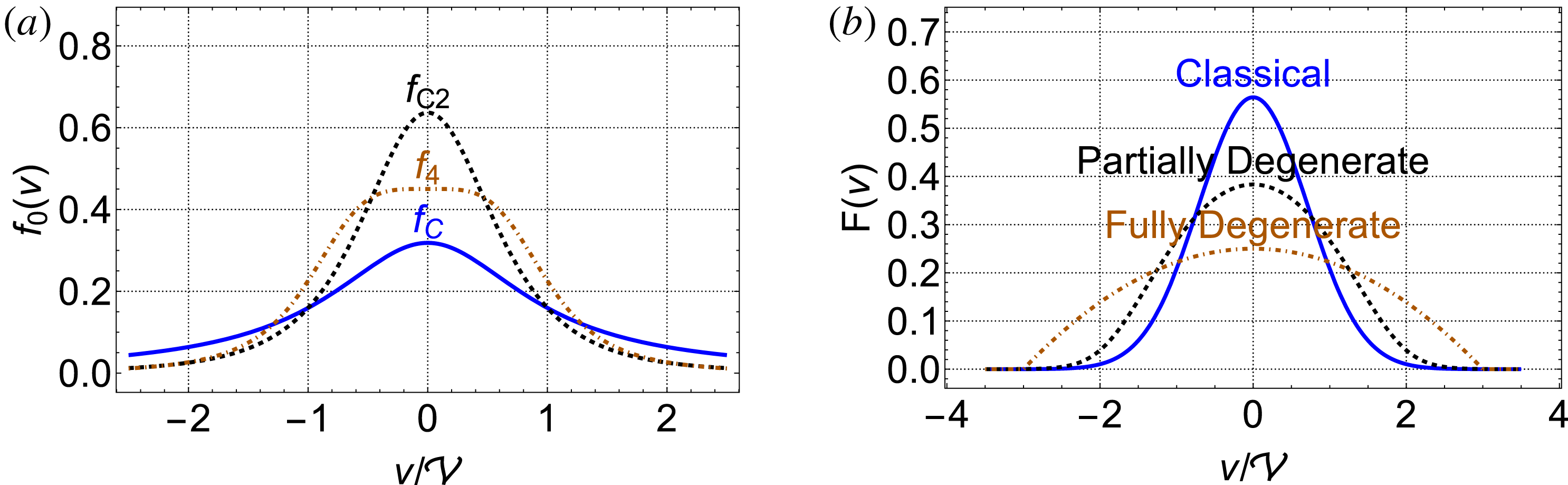
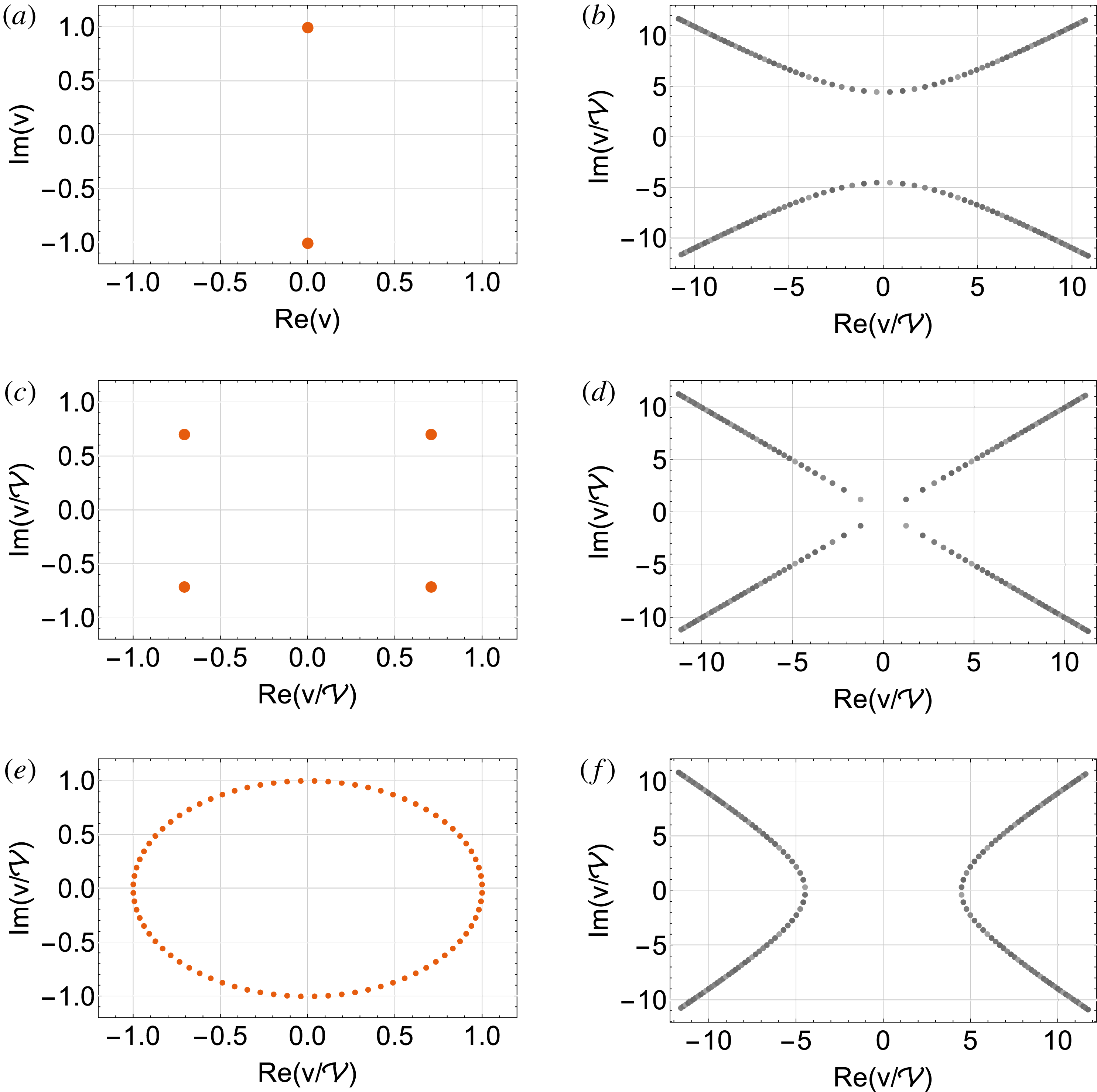
In order to better understand these distribution functions, they are plotted in figures 1(a) (Cauchy-type functions) and 1(b) (Fermi–Dirac-type functions). However, as it is necessary to evaluate these distribution functions with complex arguments, we also illustrate their structure in the complex
 $v$
plane in figure 2.
Distribution functions that are considered in this paper. Cauchy-type functions are shown in (a). The
 $f_{C2}$
function is steeper and narrower than the Cauchy function, and the
 $f_{N}$
function is broader and flatter on the top. Fermi–Dirac-type distribution functions are shown in (b), with degeneracy level ranging from classical Maxwellian to fully degenerate truncated distribution.

We now proceed to present the susceptibilities obtained by inserting the above distribution functions into (2.12). With the exception of the arbitrarily degenerate Fermi–Dirac distribution, the distributions have been chosen so that the integration of (2.12) can be carried out analytically by making use of the residue theorem. In the case of
 $f_{\unicode[STIX]{x1D6FF}}(v)$
the integration is trivial, and for
 $f_{D}$
it is carried out by standard methods with a well-defined result when the phase velocity is greater than the Fermi velocity. Smaller phase velocities result in complex logarithms for which the branch cuts must be considered carefully. The following susceptibilities are the result of these integrations:
 $$\begin{eqnarray}\displaystyle & \displaystyle \unicode[STIX]{x1D712}_{\unicode[STIX]{x1D6FF}}(\unicode[STIX]{x1D714},k)=\frac{\unicode[STIX]{x1D714}_{p}^{2}}{{k^{4}\hbar }^{2}/m^{2}-\unicode[STIX]{x1D714}^{2}}; & \displaystyle\end{eqnarray}$$
 $$\begin{eqnarray}\displaystyle & \displaystyle \unicode[STIX]{x1D712}_{C}(\unicode[STIX]{x1D714},k)=\frac{\unicode[STIX]{x1D714}_{p}^{2}}{(k{\mathcal{V}}-\text{i}\unicode[STIX]{x1D714})^{2}+{k^{4}\hbar }^{2}/m^{2}}; & \displaystyle\end{eqnarray}$$
 $$\begin{eqnarray}\displaystyle & \displaystyle \unicode[STIX]{x1D712}_{C2}(\unicode[STIX]{x1D714},k)=\frac{\unicode[STIX]{x1D714}_{p}^{2}({k^{4}\hbar }^{2}/m^{2}+3k^{2}{\mathcal{V}}^{2}-4\text{i}k{\mathcal{V}}\unicode[STIX]{x1D714}-\unicode[STIX]{x1D714}^{2})}{[(k{\mathcal{V}}-\text{i}\unicode[STIX]{x1D714})^{2}+{k^{4}\hbar }^{2}/m^{2}]^{2}}; & \displaystyle\end{eqnarray}$$
 $$\begin{eqnarray}\displaystyle \unicode[STIX]{x1D712}_{4}(\unicode[STIX]{x1D714},k) & = & \displaystyle \frac{\text{i}m^{2}\unicode[STIX]{x1D714}_{p}^{2}}{\sqrt{2}}\nonumber\\ \displaystyle & & \displaystyle \times \,[\,((-1)^{3/4}{k^{4}\hbar }^{2}+\sqrt[4]{-1}k^{2}m^{2}{\mathcal{V}}^{2}+2km^{2}{\mathcal{V}}\unicode[STIX]{x1D714}-(-1)^{3/4}m^{2}\unicode[STIX]{x1D714}^{2})^{-1}\nonumber\\ \displaystyle & & \displaystyle +\,(\sqrt[4]{-1}{k^{4}\hbar }^{2}+(-1)^{3/4}k^{2}m^{2}{\mathcal{V}}^{2}+2km^{2}{\mathcal{V}}\unicode[STIX]{x1D714}-\sqrt[4]{-1}m^{2}\unicode[STIX]{x1D714}^{2})^{-1}];\end{eqnarray}$$
 $$\begin{eqnarray}\displaystyle \unicode[STIX]{x1D712}_{CJ}(\unicode[STIX]{x1D714},k)=\unicode[STIX]{x03C0}\text{i}\frac{\unicode[STIX]{x1D714}_{p}^{2}}{k^{3}}\frac{{\mathcal{V}}^{2J-1}\unicode[STIX]{x1D6E4}(J)}{\sqrt{\unicode[STIX]{x03C0}}\unicode[STIX]{x1D6E4}\left(J-\displaystyle \frac{1}{2}\right)}\text{Res}\left[\frac{1}{(v^{2}+{\mathcal{V}}^{2})^{J}}\frac{1}{v-\unicode[STIX]{x1D714}/k},\text{i}{\mathcal{V}}\right]; & & \displaystyle\end{eqnarray}$$
 $$\begin{eqnarray}\displaystyle \unicode[STIX]{x1D712}_{J}(\unicode[STIX]{x1D714},k) & = & \displaystyle \mathop{\sum }_{j=1}^{J/2}(-\text{i})\sin \left(\frac{\unicode[STIX]{x03C0}}{J}\right)\nonumber\\ \displaystyle & & \displaystyle \times \left[(-1)^{(1-2j)/J}\left(\frac{{k^{4}\hbar }^{2}}{m^{2}\unicode[STIX]{x1D714}_{p}^{2}}-\frac{\unicode[STIX]{x1D714}^{2}}{\unicode[STIX]{x1D714}_{p}^{2}}\right)+\frac{k^{2}{\mathcal{V}}^{2}(-1)^{(2j+J-1)/J}}{\unicode[STIX]{x1D714}_{p}^{2}}-\frac{2k{\mathcal{V}}\unicode[STIX]{x1D714}}{\unicode[STIX]{x1D714}_{p}^{2}}\right]^{-1};\nonumber\\ \displaystyle & & \displaystyle\end{eqnarray}$$
and, in agreement with Krivitskii & Vladimirov (Reference Krivitskii and Vladimirov1991), Eliasson & Shukla (Reference Eliasson and Shukla2010), Vladimirov & Tyshetskiy (Reference Vladimirov and Tyshetskiy2011)
 $$\begin{eqnarray}\displaystyle & & \displaystyle \unicode[STIX]{x1D712}_{D}(\unicode[STIX]{x1D714},k)=\frac{3m}{8\hbar k{\mathcal{V}}}\left(\frac{\unicode[STIX]{x1D714}_{p}}{k{\mathcal{V}}}\right)^{2}\nonumber\\ \displaystyle & & \displaystyle \qquad \times \left[4\hbar k{\mathcal{V}}/m+(\unicode[STIX]{x1D714}/k-\hbar k/m+{\mathcal{V}})(\unicode[STIX]{x1D714}/k-\hbar k/m-{\mathcal{V}})\log \left(\frac{\hbar k/m-{\mathcal{V}}-\unicode[STIX]{x1D714}/k}{\hbar k/m+{\mathcal{V}}-\unicode[STIX]{x1D714}/k}\right)\right.\nonumber\\ \displaystyle & & \displaystyle \qquad -\left.(\unicode[STIX]{x1D714}/k+\hbar k/m-{\mathcal{V}})(\unicode[STIX]{x1D714}/k+\hbar k/m+{\mathcal{V}})\log \left(\frac{\hbar k/m+{\mathcal{V}}+\unicode[STIX]{x1D714}/k}{\hbar k/m-{\mathcal{V}}+\unicode[STIX]{x1D714}/k}\right)\right].\end{eqnarray}$$
3.2 Dispersion relations in single-population plasmas
Before proceeding to the case of multiple populations, we present the dispersion relation in single-population plasmas obtained from solving
 $$\begin{eqnarray}\displaystyle 0=1+\unicode[STIX]{x1D712}_{s}. & & \displaystyle\end{eqnarray}$$
For the delta-function we obtain
 $$\begin{eqnarray}\displaystyle \frac{\unicode[STIX]{x1D714}_{\unicode[STIX]{x1D6FF}}}{\unicode[STIX]{x1D714}_{p}}=\left\{\begin{array}{@{}l@{}}\displaystyle \pm \sqrt{1+\frac{{k^{4}\hbar }^{2}}{m^{2}\unicode[STIX]{x1D714}_{p}^{2}}}\quad \\ \displaystyle \pm \frac{k^{2}\hbar }{m\unicode[STIX]{x1D714}_{p}},\quad \end{array}\right. & & \displaystyle\end{eqnarray}$$
in agreement with Haas et al. (Reference Haas, Bret and Shukla2009). Note that there is indeed no Landau damping, but there is now wave dispersion which is due entirely to quantum dynamical effects. Additionally, the second pair of modes is called zero sound (see e.g. Krivitskii & Vladimirov (Reference Krivitskii and Vladimirov1991)) and is a purely quantum effect. Due to the lack of a characteristic particle velocity scale
 ${\mathcal{V}}$
, for plotting we non-dimensionalise according to the second scheme by introducing variables
 $\unicode[STIX]{x1D714}\equiv \unicode[STIX]{x1D714}/\unicode[STIX]{x1D714}_{p}$
,
 $k\equiv \sqrt{2\hbar /m\unicode[STIX]{x1D714}_{p}}k$
where we utilise the velocity scale
 $\unicode[STIX]{x1D702}\equiv \sqrt{2\hbar \unicode[STIX]{x1D714}_{p}/m}$
which is the speed of an electron with kinetic energy equal to the plasmon energy
 $\hbar \unicode[STIX]{x1D714}_{p}$
.
For the Cauchy distribution we obtain
 $$\begin{eqnarray}\displaystyle \frac{\unicode[STIX]{x1D714}_{C}}{\unicode[STIX]{x1D714}_{p}}=\left\{\begin{array}{@{}c@{}}\pm \sqrt{1+\displaystyle \frac{{k^{4}\hbar }^{2}}{m^{2}\unicode[STIX]{x1D714}_{p}^{2}}}-\displaystyle \frac{\text{i}k{\mathcal{V}}}{\unicode[STIX]{x1D714}_{p}}=\pm \sqrt{1+H^{2}K^{4}}-\text{i}K\\ \pm \displaystyle \frac{k^{2}\hbar }{m\unicode[STIX]{x1D714}_{p}}-\displaystyle \frac{\text{i}k{\mathcal{V}}}{\unicode[STIX]{x1D714}_{p}}=HK^{2}-\text{i}K\end{array}\right. & & \displaystyle\end{eqnarray}$$
in agreement with Haas et al. (Reference Haas, Manfredi and Goedert2001). There is now Landau damping, with the damping rate simply equal to the dimensionless wavenumber
 $K$
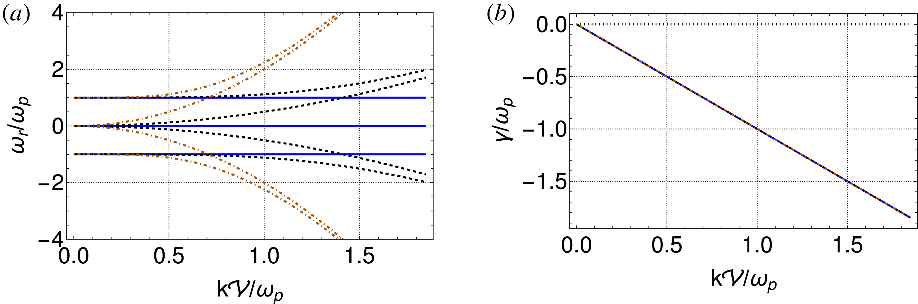
, but the real part of the frequency is the same as for the delta-function case. This dispersion relation is plotted in figure 3.
Poles of the distribution functions considered in this paper in the complex-velocity space. Panels on the left (red points) show poles of Cauchy-type distributions
 $(v^{J}+{\mathcal{V}}^{J})^{-1}$
for
 $J=2,4,80$
(a,c,e) and panels on the right (grey points) show poles of the Fermi–Dirac
 $f_{FD}(v)$
(3.10) for
 $\unicode[STIX]{x1D707}/T=-20,0,20$
(b,d,f).

For the more complicated distribution functions
 $\unicode[STIX]{x1D712}_{CJ}$
and
 $\unicode[STIX]{x1D712}_{J}$
, there is not an explicit algebraic solution for the frequency as the susceptibilities are all of greater than fourth order in
 $\unicode[STIX]{x1D714}$
. Instead, we examine the dielectric functions in the limits of large and small
 $K$
, and in the case of
 $\unicode[STIX]{x1D712}_{J}$
we can consider the case
 $J\gg 1$
. In the long-wavelength
 $K\ll 1$
limit, to fourth order, for the squared Cauchy distribution the regular plasmon mode is
 $$\begin{eqnarray}\displaystyle \unicode[STIX]{x1D6FA}_{C2}=1+\frac{3}{2}K^{2}-4\text{i}K^{3}+\left(\frac{H^{2}}{2}-\frac{105}{8}\right)K^{4}, & & \displaystyle\end{eqnarray}$$
and for the
 $J=4$
inverse-quartic distribution it is
 $$\begin{eqnarray}\displaystyle \unicode[STIX]{x1D6FA}_{4}=1+\frac{3}{2}K^{2}-2\sqrt{2}\text{i}K^{3}+\left(\frac{H^{2}}{2}-\frac{65}{8}\right)K^{4}. & & \displaystyle\end{eqnarray}$$
Note that for both of these cases the imaginary part now only appears to third order in
 $K$
, and that quantum effects only appear at fourth order, and only in the real part of the frequency. The exact, numerically computed dispersion relations are plotted in figures 4 (squared Cauchy) and 5 (inverse-quartic).
Dispersion relations are not shown for the cases with non-meromorphic distribution functions
 $f_{D}(v)$
and
 $f_{FD}(v)$
in (3.9) and (3.10) as the focus of this work is to ascertain the influence of individual poles in the complex distribution function, but they have been studied by Rightley & Uzdensky (Reference Rightley and Uzdensky2016). Additionally, further discussion of the distribution functions
 $f_{CJ}$
(3.6) and
 $f_{J}$
(3.8) is reserved for a future work.
Dispersion relation (3.20) for single-population plasma with Cauchy distribution function
 $f_{C}$
(3.2) for three values of
 $H$
:
 $H=0$
(solid, blue),
 $H=0.5$
(dashed, black) and
 $H=2$
(dot-dashed, orange). The quantum parameter
 $H$
causes dispersion in the real part (a) of the frequency but the damping rate
 $-\unicode[STIX]{x1D6FE}$
(b) is independent of
 $H$
and equal to
 $k{\mathcal{V}}/\unicode[STIX]{x1D714}_{p}$
.

Dispersion relation for single-population plasma with squared Cauchy or
 $f_{C2}$
distribution function (3.3) for three values of
 $H$
:
 $0$
(a,b),
 $0.5$
(c,d), and
 $2$
(e,f).

Dispersion relation for single-population plasma with inverse-quartic or
 $f_{4}$
distribution function (3.4) for three values of
 $H$
:
 $0$
(a,b),
 $0.5$
(c,d), and
 $2$
(e,f).

4 Dispersion relations for two-population plasmas
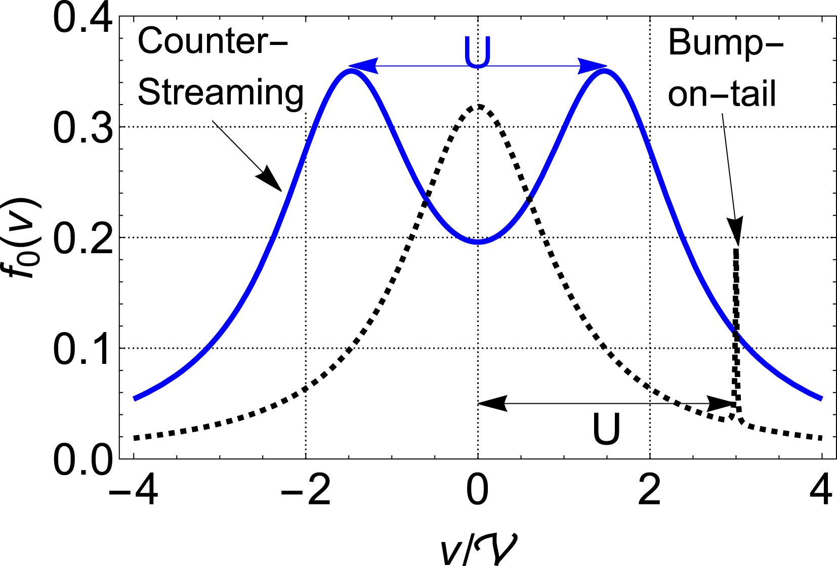
If two populations are present, we define one to be the primary population and one the secondary. The non-dimensional variables in § 2.3 are defined in terms of the primary population. In this paper, for each type of distribution function we consider two cases: Case 1 the symmetrical case: that of two identical counter-drifting populations and Case 2 the bump-on-tail case: that of a primary distribution and a drifting secondary delta-function beam. The issue of frame of reference should be addressed, as for multiple populations there is not necessarily a natural choice for this frame. In Case 1 we choose the centre-of-momentum frame, so that each population moves past the observer with speed
 $U/2$
in opposite directions, and in Case 2 we choose the reference frame of the primary (finite-width) population, with the low-density population streaming by at speed
 $U$
in the positive direction. The difference between Cases 1 and 2 is shown in figure 6.
The dielectric function for Case 1 is
 $$\begin{eqnarray}\displaystyle \unicode[STIX]{x1D716}_{1}=1+{\textstyle \frac{1}{2}}[\unicode[STIX]{x1D712}_{s}(\unicode[STIX]{x1D714}+kU/2,k)+\unicode[STIX]{x1D712}_{s}(\unicode[STIX]{x1D714}-kU/2,k)], & & \displaystyle\end{eqnarray}$$
with the factor
 $1/2$
ensuring the total density is equal to unity. The dielectric function for Case 2 is
 $$\begin{eqnarray}\displaystyle \unicode[STIX]{x1D716}_{2}=1+[(1-n)\unicode[STIX]{x1D712}_{s}(\unicode[STIX]{x1D714},k)+n\unicode[STIX]{x1D712}_{\unicode[STIX]{x1D6FF}}(\unicode[STIX]{x1D714}-kU,k)], & & \displaystyle\end{eqnarray}$$
where the quantity
 $n$
is the fraction of particles present in the beam.
Two-population distribution functions for symmetrical case (solid, blue) and for bump-on-tail case (dashed, black). The separation velocity between the two populations is denoted by
 $U$
.

As in the classical case, two-population plasmas may allow for unstable modes, at least for large enough velocity separations
 $U$
. For each distribution function and case, we will be mapping the boundaries of the region(s) of instability in the
 $(k,U)$
parameter space. We denote the critical value of drift velocity required for the onset of instability as
 $U_{\text{crit}}$
. If a configuration with given
 $U$
allows for an unstable mode, we name the maximum growth rate of this mode
 $\unicode[STIX]{x1D6FE}_{\max }(U)$
and the wavenumber at which this occurs
 $k_{\max }(U)$
. As will be seen, for fixed
 $U$
there exist up to three critical values of
 $k$
which define the boundaries (
 $\unicode[STIX]{x1D6FE}=0$
) of the unstable region, and we label these (in order of increasing value of
 $k$
)
 $k_{1}$
,
 $k_{2}$
and
 $k_{3}$
. In the classical case instability exists only for long enough wavelengths
 $k<k_{1}$
. In contrast, in the quantum case for large enough values of the quantum recoil parameter there are two instability windows
 $k<k_{1}$
and
 $k_{2}<k<k_{3}$
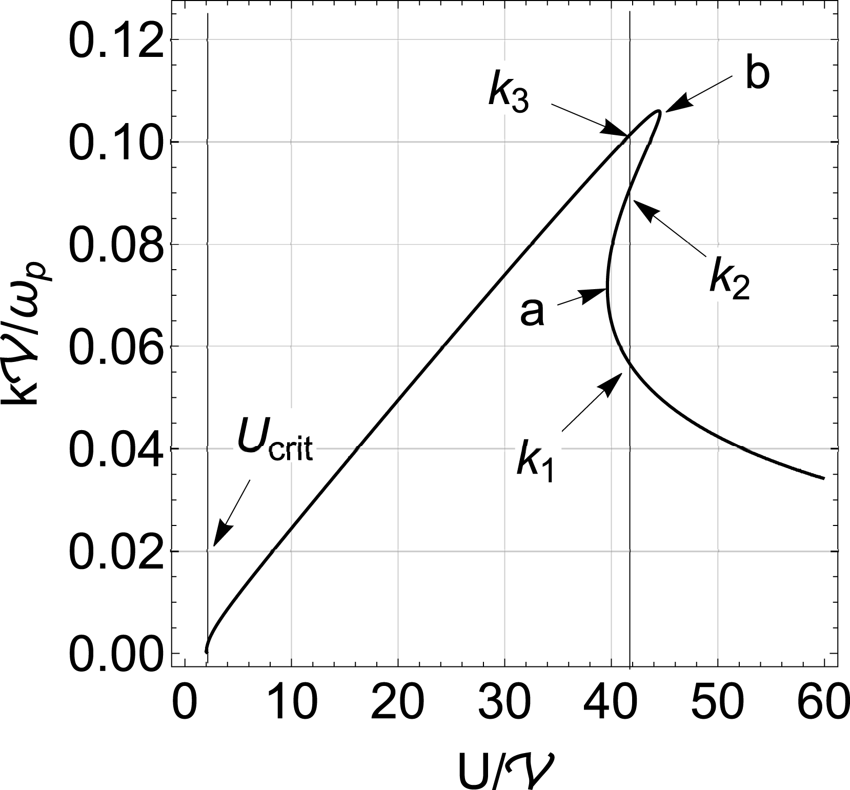
. In addition, there are two further special points denoted a and b that define the extent of the instability region. These points are demonstrated in figure 7.
Example boundary of instability region, for symmetrical counter-propagating Cauchy distributions with
 $H=150$
. The Cauchy distribution is used for illustration but the other distributions considered in this paper result in the same general features. The unstable region is under the curve. For given
 $U$
, instability exists for
 $0<k<k_{1}$
and
 $k_{2}<k<k_{3}$
. Point a refers to the drift speed
 $U_{a}$
beyond which the second region of instability defined by
 $k_{2}$
and
 $k_{3}$
ceases to exist when
 $k_{2}$
and
 $k_{3}$
merge. Point b refers to the minimum drift speed
 $U_{b}$
needed for the existence of the second region of instability, at which point
 $k_{1}$
and
 $k_{2}$
merge.
 $U_{\text{crit}}$
refers to the minimum drift speed required for the existence of any instability.

4.1 Delta-function distribution: most simple case
To begin, we consider a two-population plasma in which both populations have zero velocity spread; i.e. Dirac delta-function distributions. In Case 1 both populations are identical, and in Case 2 the populations have unequal total particle densities, with one beam being substantially less dense.
4.1.1 Case 1: symmetrically counter-propagating distributions
For Dirac delta-function distributions, in the centre-of-mass frame, utilising (3.11) we have
 $$\begin{eqnarray}\displaystyle \unicode[STIX]{x1D750}=1-\frac{1}{2}\left\{\frac{\unicode[STIX]{x1D714}_{p}^{2}}{(\unicode[STIX]{x1D714}-kU/2)^{2}-{k^{4}\hbar }^{2}/m^{2}}+\frac{\unicode[STIX]{x1D714}_{p}^{2}}{(\unicode[STIX]{x1D714}+kU/2)^{2}-{k^{4}\hbar }^{2}/m^{2}}\right\}. & & \displaystyle\end{eqnarray}$$
In this case the dispersion relation
 $\unicode[STIX]{x1D716}=0$
can be solved exactly and is
 $$\begin{eqnarray}\displaystyle \frac{\unicode[STIX]{x1D714}_{\pm \pm }}{\unicode[STIX]{x1D714}_{p}}=\frac{1}{2}\left\{\!\left(\frac{kU}{\unicode[STIX]{x1D714}_{p}}\right)\pm \sqrt{2+4\left(\frac{\unicode[STIX]{x1D702}k}{\unicode[STIX]{x1D714}_{p}}\right)^{4}\!+\left(\frac{kU}{\unicode[STIX]{x1D714}_{p}}\right)^{2}\!\pm 2\sqrt{1+2\left(\frac{kU}{\unicode[STIX]{x1D714}_{p}}\right)^{2}\left[2\left(\frac{\unicode[STIX]{x1D702}k}{\unicode[STIX]{x1D714}_{p}}\right)^{4}\!+1\right]}}\right\}. & & \displaystyle \nonumber\\ \displaystyle & & \displaystyle\end{eqnarray}$$
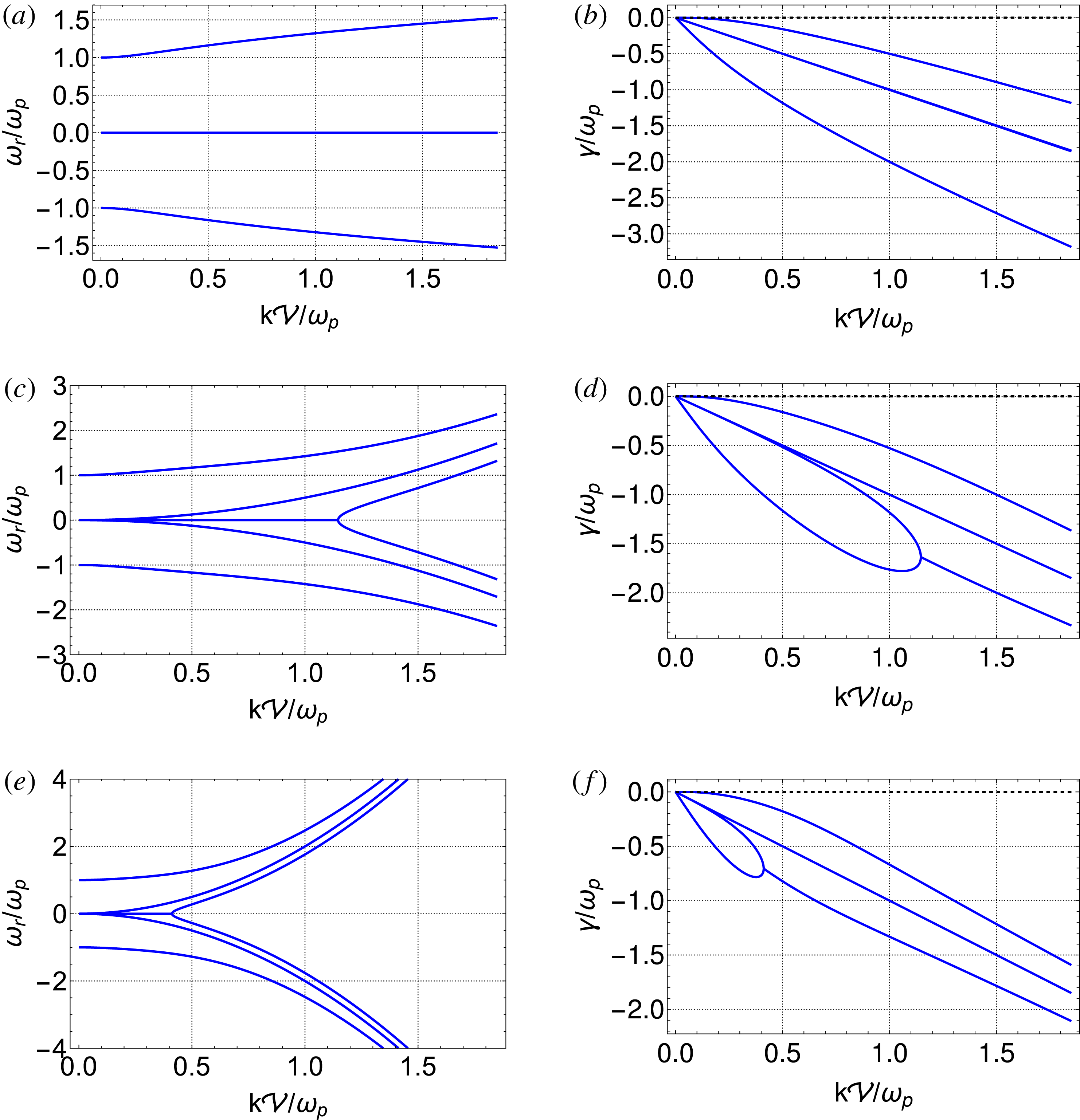
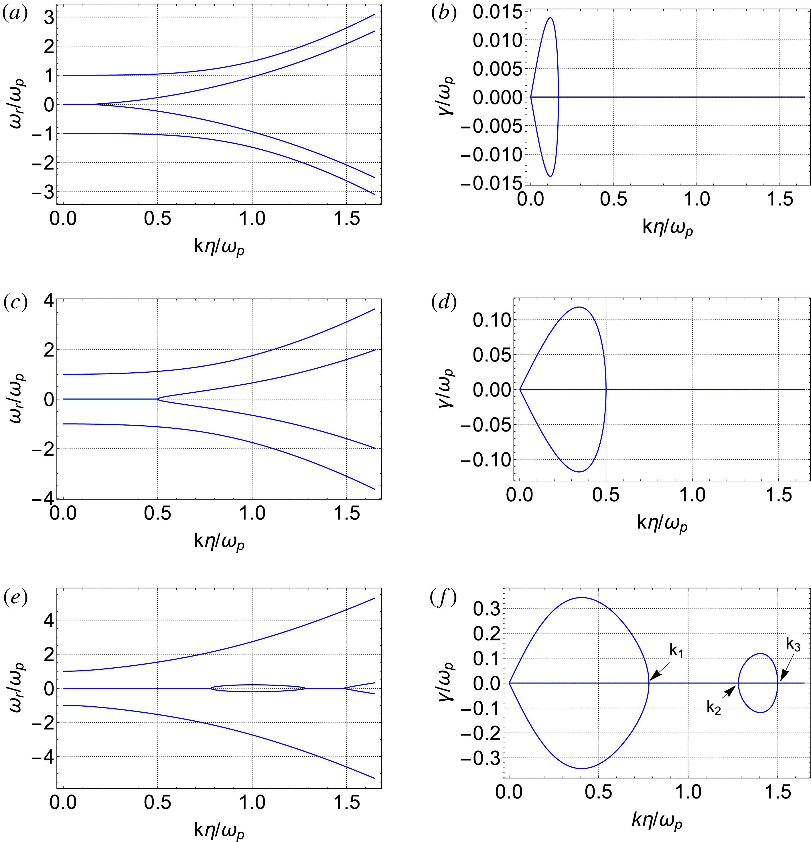
This solution is plotted in figure 8 using the second normalisation scheme from § 2.3. Expression (4.4) contains four branches: two pairs of two. Modes
 $\unicode[STIX]{x1D714}_{++}$
and
 $\unicode[STIX]{x1D714}_{-+}$
are purely real for all values of
 $U$
and become the regular plasmon modes when
 $U\rightarrow 0$
. Modes
 $\unicode[STIX]{x1D714}_{+-}$
and
 $\unicode[STIX]{x1D714}_{--}$
are purely imaginary for small enough values of
 $k$
for any
 $U$
and purely real for large
 $k$
, with mode
 $\unicode[STIX]{x1D714}_{+-}$
being positive and unstable and
 $\unicode[STIX]{x1D714}_{--}$
being negative and stable.
Dispersion relations for symmetrical counter-drifting delta-function distributions for three different values of the drift velocity
 $U$
relative to the characteristic quantum speed
 $\unicode[STIX]{x1D702}\equiv \sqrt{\hbar \unicode[STIX]{x1D714}_{p}/m_{e}}$
:
 $U=\unicode[STIX]{x1D702}/3$
(a,b),
 $U=\unicode[STIX]{x1D702}$
(c,d) and
 $U=3\unicode[STIX]{x1D702}$
(e,f). The second region of instability appears for
 $U=3\unicode[STIX]{x1D702}$
(f). This region corresponds with the crossing of modes in the plot of the real part of the frequency (e).

Focusing on the potentially unstable mode
 $\unicode[STIX]{x1D714}_{+-}$
, the values of
 $k$
for which the radical becomes zero,
 $$\begin{eqnarray}\displaystyle 2+4\left(\frac{\unicode[STIX]{x1D702}k}{\unicode[STIX]{x1D714}_{p}}\right)^{4}+\left(\frac{kU}{\unicode[STIX]{x1D714}_{p}}\right)^{2}=2\sqrt{1+2\left(\frac{kU}{\unicode[STIX]{x1D714}_{p}}\right)^{2}\left[2\left(\frac{\unicode[STIX]{x1D702}k}{\unicode[STIX]{x1D714}_{p}}\right)^{4}+1\right]}, & & \displaystyle\end{eqnarray}$$
are
 $$\begin{eqnarray}\displaystyle & \displaystyle k_{1}=\frac{2\unicode[STIX]{x1D714}_{p}}{U} & \displaystyle\end{eqnarray}$$
 $$\begin{eqnarray}\displaystyle & \displaystyle k_{2}=\frac{\unicode[STIX]{x1D714}_{p}}{2\sqrt{2}\unicode[STIX]{x1D702}}\sqrt{(U/\unicode[STIX]{x1D702})^{2}-\sqrt{(U/\unicode[STIX]{x1D702})^{4}-64}} & \displaystyle\end{eqnarray}$$
 $$\begin{eqnarray}\displaystyle & \displaystyle k_{3}=\frac{\unicode[STIX]{x1D714}_{p}}{2\sqrt{2}\unicode[STIX]{x1D702}}\sqrt{(U/\unicode[STIX]{x1D702})^{2}+\sqrt{(U/\unicode[STIX]{x1D702})^{4}-64}}. & \displaystyle\end{eqnarray}$$
The dependence of
 $k_{1}$
on
 $U$
shows that an instability exists for all non-zero values of
 $U$
, with the range of unstable wavelengths between
 $k=0$
and
 $k=k_{1}$
decreasing as
 $U$
increases. The additional region of instability exists for
 $U/\unicode[STIX]{x1D702}>\sqrt{8}$
. Referring to figure 7, this is point b, at which
 $U_{b}=\sqrt{8}\unicode[STIX]{x1D702}$
and
 $k_{b}\unicode[STIX]{x1D702}/\unicode[STIX]{x1D714}_{p}=(1/2\sqrt{2})U_{b}/\unicode[STIX]{x1D702}=1$
. The presence of the velocity
 $\unicode[STIX]{x1D702}$
means that this region is explicitly dependent on quantum phenomena. In the classical limit
 $\unicode[STIX]{x1D702}$
vanishes, and thus
 $k_{b}$
approaches infinity (the second region of instability exists only for shorter and shorter wavelengths and ultimately vanishes). For counter-streaming delta functions, point a moves out to infinity along a quantum ray of instability described by
 $k=U\unicode[STIX]{x1D714}_{p}/2\unicode[STIX]{x1D702}^{2}$
. In the limit
 $U\gg \unicode[STIX]{x1D702}$
, the region of instability is bounded by
 $k\unicode[STIX]{x1D702}/\unicode[STIX]{x1D714}_{p}<2\unicode[STIX]{x1D702}/U$
and
 $U/2\unicode[STIX]{x1D702}-4\unicode[STIX]{x1D702}^{3}/U^{3}<k\unicode[STIX]{x1D702}/\unicode[STIX]{x1D714}_{p}<U/2\unicode[STIX]{x1D702}$
. Furthermore, for
 $U\gg \unicode[STIX]{x1D702}$
the wavenumbers of maximum growth rate are
 $k_{\max }\unicode[STIX]{x1D702}/\unicode[STIX]{x1D714}_{p}=\sqrt{2}\unicode[STIX]{x1D702}/U$
with maximum growth rate
 $\unicode[STIX]{x1D714}_{p}(\sqrt{5}/2-1)^{1/2}$
, which is independent of
 $\hbar$
, and
 $k_{\max }\unicode[STIX]{x1D702}/\unicode[STIX]{x1D714}_{p}=U/2\unicode[STIX]{x1D702}-2\unicode[STIX]{x1D702}^{3}/U^{3}$
with maximum growth rate
 $\unicode[STIX]{x1D714}_{p}\unicode[STIX]{x1D702}^{2}/U^{2}$
, which is zero for
 $\hbar \rightarrow 0$
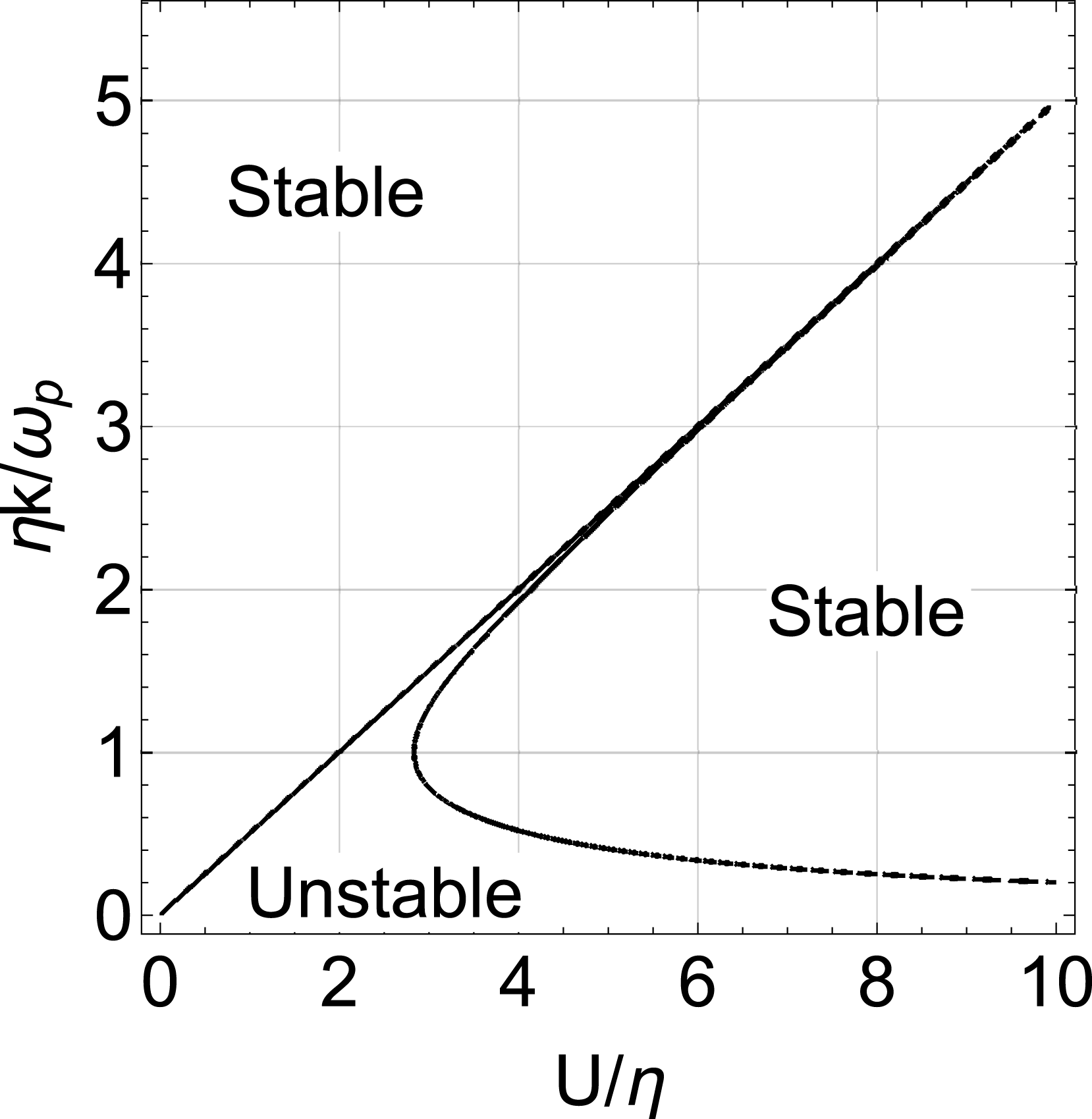
, as this second region of instability is a purely quantum effect. The region of instability is plotted in figure 9, in which one can see the
 $\propto 1/U$
and
 $\propto U$
dependence of
 $k_{1}$
and
 $k_{2},k_{3}$
, respectively.
Instability region for counter-propagating identical cold delta-function beams. The unstable region fills the region under the plotted curve.

Dispersion relations for asymmetrical counter-drifting delta-function distributions with
 $n=1/100$
with:
 $U=\unicode[STIX]{x1D702}/3$
(a,b),
 $U=\unicode[STIX]{x1D702}$
(c,d) and
 $U=3\unicode[STIX]{x1D702}$
(e,f). Again, the second region of instability exists near
 $k\approx 1.4$
for
 $U=3\unicode[STIX]{x1D702}$
(f). The effect of the decreased density of the second beam leads to a decrease in the values of
 $k_{1}$
, and the difference between
 $k_{2}$
and
 $k_{3}$
decreases.

4.1.2 Case 2: primary delta-function population with delta-function beam of arbitrary density
In Case 2 the two delta functions do not have equal density, the symmetry is broken and the general solution for the dispersion relation is quite complicated and there is little to be gained by looking at the full solution. Instead, here we focus on the small
 $k$
(long wavelength) limit of the dispersion relation, and on numerically obtained roots. The exact dispersion relation for this case is plotted in figure 10, where it is seen that both the first and second regions of instability are diminished in domain and range, and there is dispersion due to the Doppler shift into the frame of the primary beam. However, the behaviour is qualitatively similar to Case 1. In the limit
 $\unicode[STIX]{x1D702}k/\unicode[STIX]{x1D714}_{p}\ll 1$
the unstable root is
 $$\begin{eqnarray}\displaystyle \frac{\unicode[STIX]{x1D714}}{\unicode[STIX]{x1D714}_{p}}=\text{i}\frac{k\unicode[STIX]{x1D702}}{\unicode[STIX]{x1D714}_{p}}\frac{U}{\unicode[STIX]{x1D702}}(\sqrt{(3-n)n}+\text{i}n)+O(k^{2}), & & \displaystyle\end{eqnarray}$$
which is always unstable since
 $n$
is constrained to be less than 1. This is independent of
 $\hbar$
up to this order. For a weak beam (
 $n\ll 1$
) the growth rate is
 $$\begin{eqnarray}\displaystyle \frac{\unicode[STIX]{x1D6FE}}{\unicode[STIX]{x1D714}_{p}}\approx \frac{kU}{\unicode[STIX]{x1D714}_{p}}\sqrt{3n}, & & \displaystyle\end{eqnarray}$$
which is linear in
 $k$
and grows as the square root of
 $n$
.
There is an additional new behaviour when
 $n$
is sufficiently small. For
 $n$
smaller than approximately
 $1/500$
, a third window of unstable wavenumbers appears for certain values of
 $U$
. This behaviour is demonstrated in figure 11, where (b) shows the behaviour of
 $\unicode[STIX]{x1D6FE}$
as a function of
 $k$
for fixed
 $U$
. Further information can be gained from figure 12, where the region of instability is plotted as a function of
 $k$
and
 $U$
for fixed
 $n=1/1000$
. In this figure, it is seen that for smaller
 $n$
the region of instability curves towards smaller
 $U$
as
 $k$
increases, and then curves back and follows the behaviour of the
 $n=100$
case for sufficiently large
 $k$
. The critical value of
 $n$
for the onset of this phenomenon could not be determined in this work and remains an open question.
Dispersion relation for asymmetrical counter-drifting delta-function distributions with
 $n=1/1000$
and
 $U=3\unicode[STIX]{x1D702}$
. The third region of instability is seen in (b), and is associated with an additional crossing between modes in (a).

Instability region for counter-propagating asymmetrical cold delta-function beams, with
 $n=1/1000$
. The unstable region fills the region under the plotted curve, and demonstrates the existence of a third region of unstable values for
 $k$
when
 $U$
is between
 $2.2$
and
 $4$
. This is due to the curving backwards of the window of instability for intermediate values of
 $k$
as
 $n$
is diminished.

4.2 Cauchy distribution: most simple case with Landau damping
For the Cauchy distribution the resulting susceptibility is given by (3.12). In this and the following subsections we will employ our normalisation scheme 1 from § 2.3, and correspondingly will measure the separation velocity
 $U$
in units of the width
 ${\mathcal{V}}$
and encapsulate quantum effects in the parameter
 $H=\hbar \unicode[STIX]{x1D714}_{p}/m{\mathcal{V}}^{2}$
. The finite width of the Cauchy distribution allows for Landau damping, and we will see that, as in the single-population case discussed in § 3, the only modification to the dispersion relation is the addition of the Landau damping term. However, this reduces the region of instability by providing an additional negative component to the imaginary part of
 $\unicode[STIX]{x1D714}$
.
4.2.1 Case 1: symmetrically counter-propagating distributions
In Case 1 there is again a simple closed form solution for the dispersion relation,
 $$\begin{eqnarray}\displaystyle \unicode[STIX]{x1D6FA}=\pm {\textstyle \frac{1}{2}}\sqrt{2+4H^{2}K^{4}+U^{2}K^{2}\pm 2\sqrt{1+2K^{2}U^{2}(2H^{2}K^{4}+1)}}-\text{i}K. & & \displaystyle\end{eqnarray}$$
This is plotted in figure 13. Equation (4.11) is nearly identical to the dispersion relation (4.4) in the previously considered scenario, but with the additional term
 $-\text{i}k{\mathcal{V}}/\unicode[STIX]{x1D714}_{p}$
reflecting that every mode experiences Landau damping. The similarity to the delta-function case can be attributed to the lack of dispersion in a Cauchy plasma due to the lack of a finite pressure. Additionally, the second region of instability ceases to exist for large enough
 $U$
, terminating at point a (see figure 7). For large
 $U$
the instability boundary is defined by
 $$\begin{eqnarray}\displaystyle K_{1}\approx \frac{2}{U}-\frac{12}{U^{3}}+\frac{16H^{2}+44}{U^{5}}, & & \displaystyle\end{eqnarray}$$
where quantum effects appear at fourth order in
 ${\mathcal{V}}/U$
. The maximum growth rate occurs at
 $$\begin{eqnarray}\displaystyle K_{\max }\approx \frac{\sqrt{2}}{U}+\frac{\sqrt{3}}{U^{2}}-\frac{9}{2\sqrt{2}U^{3}}+\frac{3\sqrt{3}}{U^{4}}+\frac{256H^{2}-225}{16\sqrt{2}U^{5}}, & & \displaystyle\end{eqnarray}$$
with maximum growth rate
 $$\begin{eqnarray}\displaystyle \frac{\unicode[STIX]{x1D6FE}_{\max }}{\unicode[STIX]{x1D714}_{p}}\approx \frac{1}{2\sqrt{3}}-\frac{\sqrt{2}}{U}-\frac{3\sqrt{3}}{2U^{2}}+\frac{15}{2\sqrt{2}U^{3}}+\frac{(16H^{2}-63)}{4\sqrt{3}U^{4}}. & & \displaystyle\end{eqnarray}$$
It is apparent that quantum effects appear at fourth order in
 $U^{-1}$
.
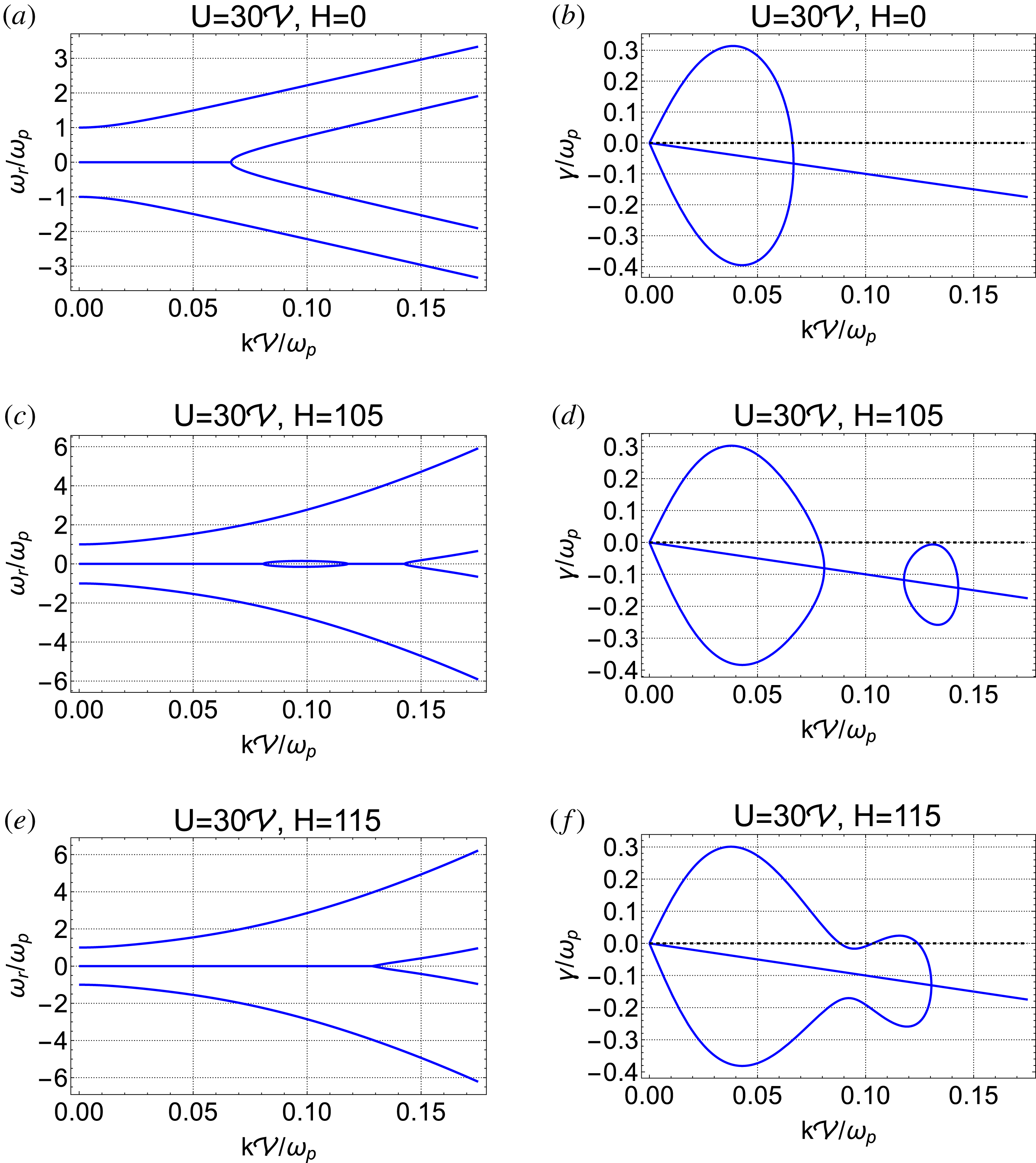
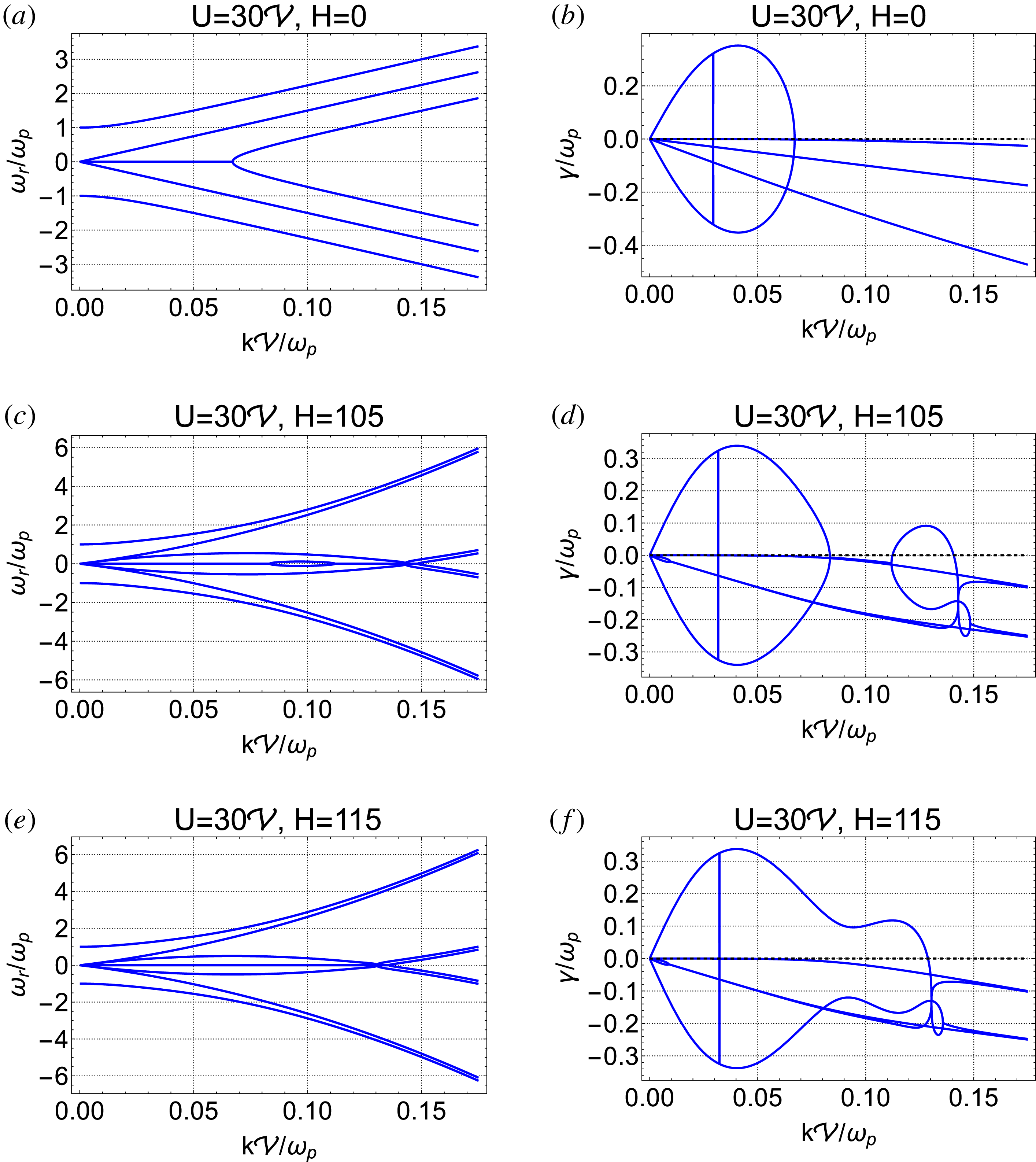
Dispersion relations for symmetrical counter-drifting Cauchy distribution functions (Case 1). The behaviour is similar to that of the delta-function distributions as seen in figure 8. The presence of Landau damping in the Cauchy distribution case decreases the maximum growth rates and diminishes the ranges of
 $k$
for which instability exists. The ‘bubble’ in (d) moves towards smaller
 $k$
as
 $H$
increases and is responsible for the second region of instability defined by
 $k_{2}$
and
 $k_{3}$
in figure 7. In (f) this ‘bubble’ merges with the primary instability region.

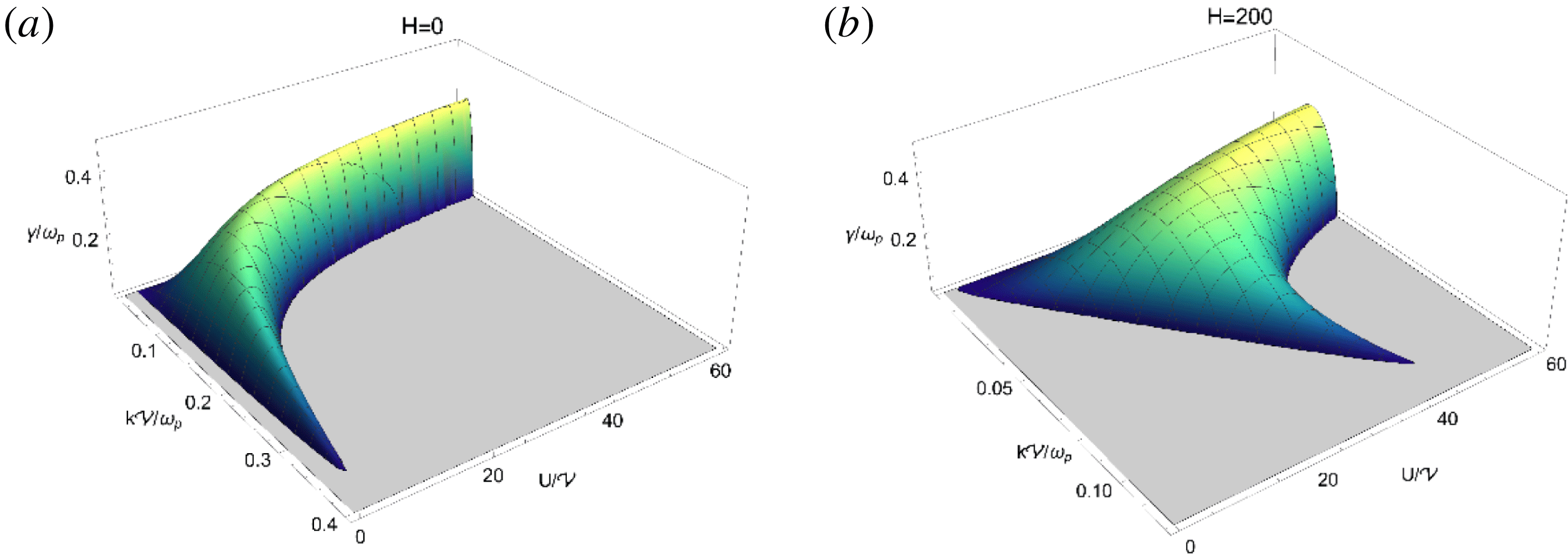
The boundary of the region of instability is shown in figure 15 and the growth rate in the unstable region is shown in figure 16, which demonstrate similar behaviour to the case of counter-drifting delta functions with the following difference. Importantly, the instability region does not extend to arbitrarily small
 $U$
or arbitrarily large
 $K$
. This shows that for finite-width distribution functions instability only occurs when the populations are separated by sufficiently large drift velocity. This is also shown by expanding for small
 $K$
. The boundary of the instability region for small
 $K$
is given by
 $$\begin{eqnarray}\displaystyle K_{1}\approx \frac{2\sqrt{U^{2}-4}(U^{2}+4)}{\sqrt{(U^{2}+4)^{4}-16H^{2}(U^{4}-24U^{2}+16)}}, & & \displaystyle\end{eqnarray}$$
with the classical limit
 $$\begin{eqnarray}\displaystyle K_{1}=\frac{2\sqrt{U^{2}-4}}{U^{2}+4} & & \displaystyle\end{eqnarray}$$
from which it can be shown that the instability exists only for
 $U>2$
in both the classical and quantum cases. In this regime the max growth rate is found at
 $$\begin{eqnarray}\displaystyle K_{\max }\approx \sqrt{\frac{2}{3}}\sqrt{\frac{(U-2)U}{4H^{2}+U^{4}}}, & & \displaystyle\end{eqnarray}$$
with growth rate
 $$\begin{eqnarray}\displaystyle \frac{\unicode[STIX]{x1D6FE}_{\max }}{\unicode[STIX]{x1D714}_{p}}\approx \frac{1}{3}\sqrt{\frac{2}{3}}(U-2)\sqrt{\frac{(U-2)U}{4H^{2}+U^{4}}}. & & \displaystyle\end{eqnarray}$$
Unfortunately, we are unable to obtain analytical expressions for the behaviour of the second region of instability, as there is no small parameter in this region, but it is apparent from the full solution obtained numerically in figure 15 that both
 $K_{a}$
and
 $K_{b}$
decrease with
 $H$
, and
 $U_{a}$
and
 $U_{b}$
increase with
 $H$
. This means the range from
 $K_{1}$
to
 $K_{2}$
decreases with
 $H$
, while the range of velocities
 $U_{b}-U_{a}$
increases with
 $H$
. The second region of instability appears for
 $H\sim 50$
. A determination of the precise critical value of
 $H$
could not be carried out in this work.
Dispersion relations for primary Cauchy distribution function population with low-density drifting beam with
 $n=1/100$
(Case 2). The modes are quantitatively altered from that of the symmetrical case in figure 13. However, the general behaviour is the same, with a region of instability for
 $k<k_{1}$
and a second, quantum, region of instability for
 $k_{2}<k<k_{3}$
for large enough
 $H$
.

Region of instability for the dispersion relation for Case 1 (counter-drifting Cauchy distributions), equation (4.11) for
 $H=0$
,
 $30$
,
 $75$
and
 $250$
(labelled in figure). The second region of instability emerges for
 $H\gtrsim 50$
, and its existence is thus reliant on sufficient strong quantum effects.

Dispersion relation for the imaginary part of the frequency with counter-streaming Cauchy distributions in Case 1, equation (4.11). The unstable region is shown, with
 $H=0$
(a) and
 $H=200$
(b).

4.2.2 Case 2: primary population with delta-function beam
Similarly to the delta-function beams, in Case 2 there is no simple solution for the dispersion relation. However, the asymptotic behaviour of
 $\unicode[STIX]{x1D714}$
can still be determined. In the small-
 $K$
limit the unstable mode is
 $$\begin{eqnarray}\displaystyle \unicode[STIX]{x1D714}\approx -kn(U+\text{i})+\text{i}k\sqrt{n}(U+\text{i})+kU+O(K^{2}), & & \displaystyle\end{eqnarray}$$
which is unstable for arbitrarily small values of
 $U$
. The numerically obtained dispersion relation for this asymmetrical case is plotted in figure 14. The distinction in comparison to Case 1 is more notable here than for the delta functions, in that the damping of the unstable mode for
 $K>K_{1}$
disappears. However, the existence of one region of instability for small
 $H$
and the appearance of a second window for sufficiently large
 $H$
remain as important features.
The behaviour of the modes shown in figure 14 differs from that in Case 1 in part due to the change in frame of reference, which Doppler shifts the real part of the frequency and accounts for the phase velocity of the unstable mode for
 $k<k_{1}$
being equal to the beam velocity. Additionally, the ‘bubble’ in the plot of
 $\unicode[STIX]{x1D6FE}$
in figure 13(d,f) is not present, but the second region of instability still exists. The ‘bubble’ instead is split by the difference in Landau damping rate between the two modes.
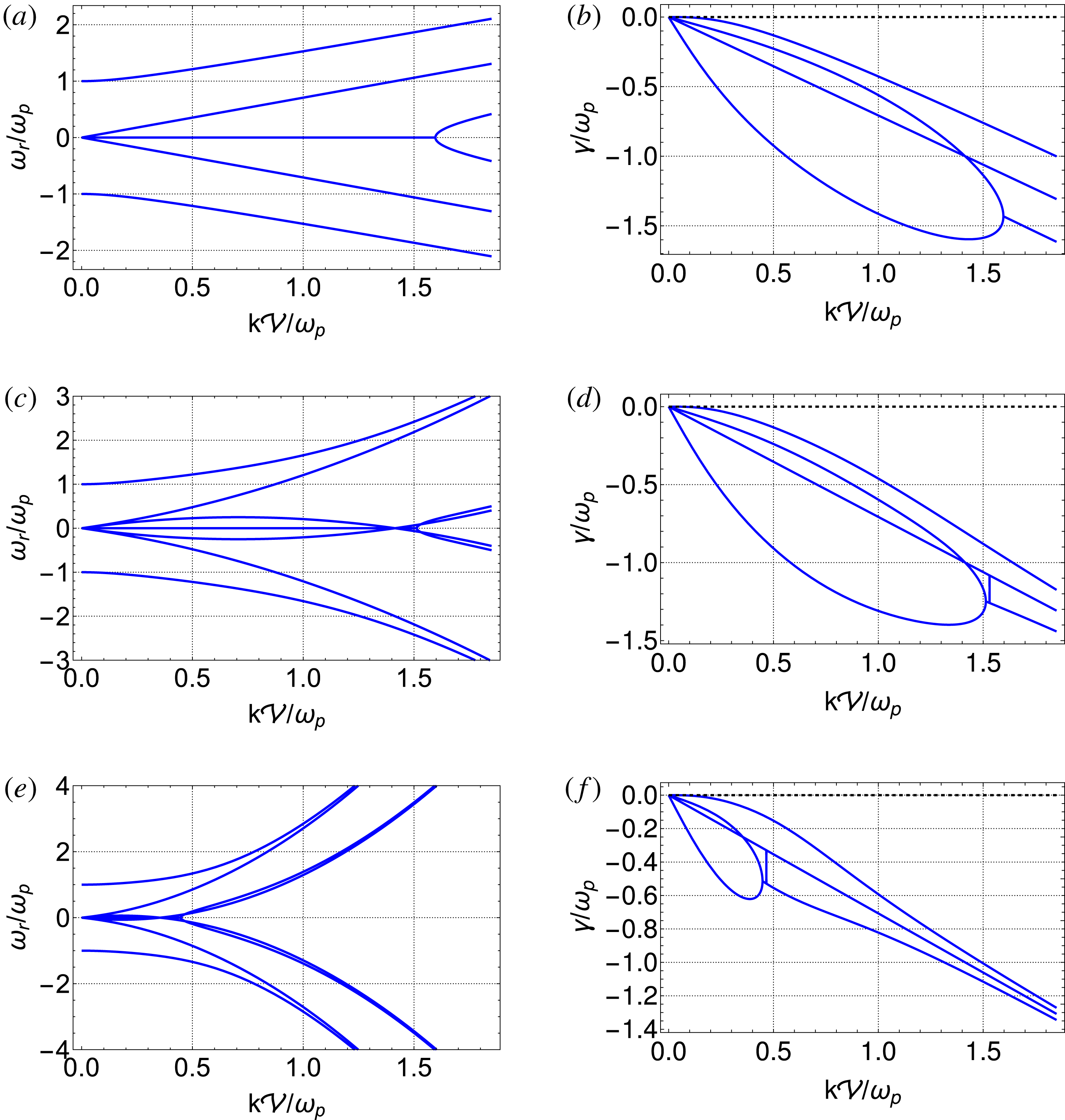
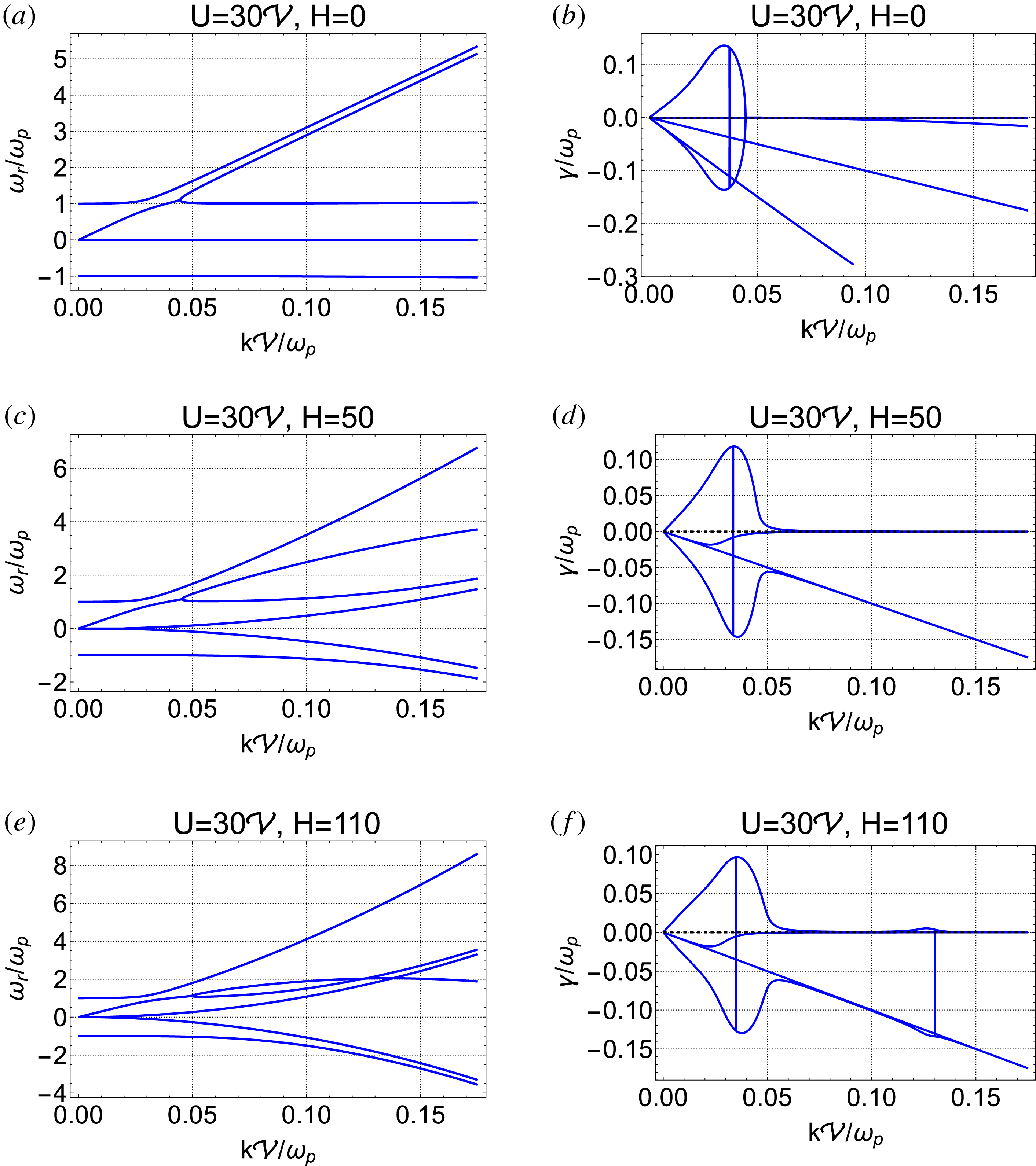
Exact dispersion relations for the symmetrical counter-drifting squared Cauchy distribution functions (Case 1). The behaviour is generally similar to that of the Cauchy distributions as seen in figure 13, with the existence of a pair of new modes which interact with the unstable mode at the point where the second region of instability terminates (i.e.
 $k_{3}$
).

Exact dispersion relations for primary squared Cauchy distributed population with low-density drifting beam with
 $n=1/100$
(Case 2). The asymptotic behaviour is different from Case 1 (figure 17) in that the plot of
 $\unicode[STIX]{x1D714}$
is Doppler shifted due to the change reference frames, and the unstable mode becomes an undamped plasma oscillation for large wavenumbers. This can be interpreted as a stationary oscillation in the beam, which explains the lack of Landau damping.

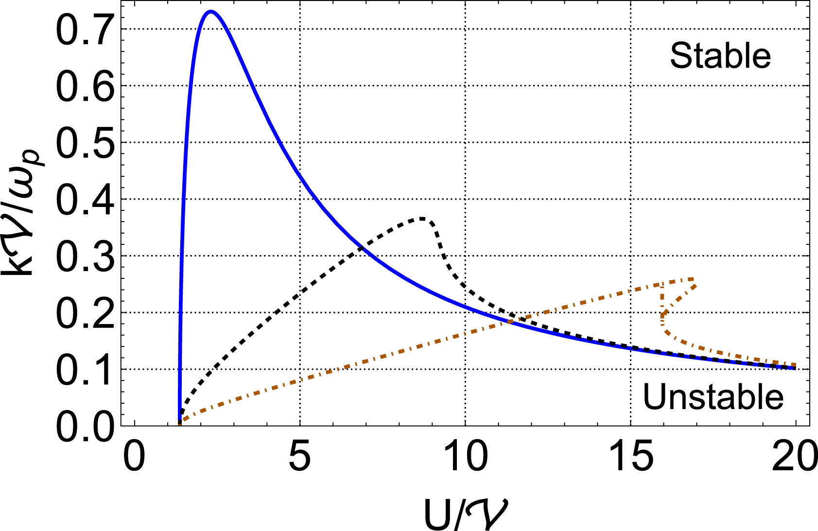
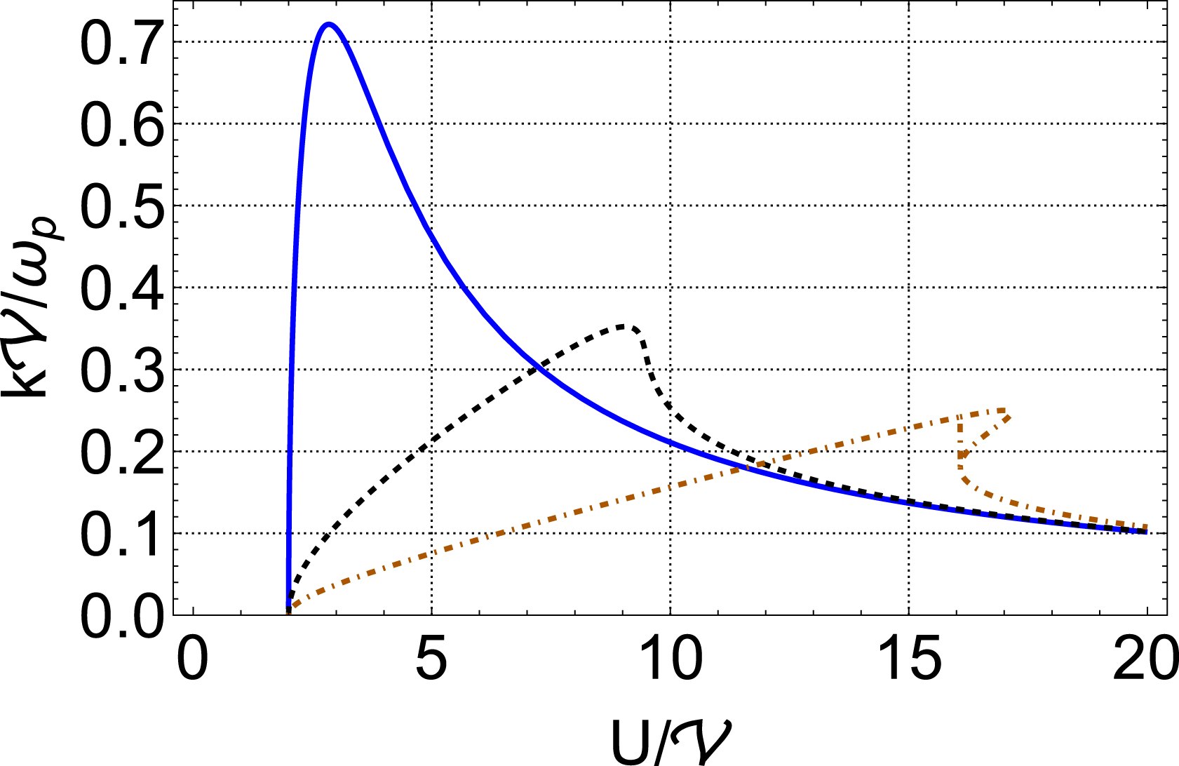
Region of instability for the dispersion relation for counter-streaming squared Cauchy distributions with
 $H=0$
, (blue solid),
 $H=10$
(black dashed) and
 $H=30$
(orange dot-dashed). The second region of instability is seen to emerge for smaller
 $H$
than for the counter-drifing Cauchy distributions.

4.3 Squared Cauchy distribution: case with classical dispersion
The primary physical difference between the squared Cauchy distribution and the Cauchy distribution is that it has a finite second moment. This means that there can be thermal dispersion of the electrostatic waves, which we do not see for the Cauchy case. Due to the presence of a velocity scale
 ${\mathcal{V}}$
associated with the distribution function, we utilise the first normalisation scheme discussed in § 2.3.
4.3.1 Case 1: symmetrically counter-propagating distributions
The dispersion relation for Case 1 can only be obtained analytically under approximations of
 $U\gg {\mathcal{V}}$
or
 $K\ll 1$
, but the roots of
 $\unicode[STIX]{x1D716}(\unicode[STIX]{x1D6FA},K)$
can be found numerically for any values of
 $K$
and
 $U$
. We first consider the case
 $U\gg {\mathcal{V}}$
in which case the dispersion relation is
 $$\begin{eqnarray}\displaystyle \unicode[STIX]{x1D6FA}\approx \frac{K\sqrt{K^{2}(U^{4}-16)-4(U^{2}+12^{2})}}{4\sqrt{3}}. & & \displaystyle\end{eqnarray}$$
In this limit, the region of instability is bounded by
 $$\begin{eqnarray}\displaystyle K_{1}\approx \frac{2}{U}+\frac{12}{U^{3}}+\frac{4(4H^{2}-69)}{U^{5}}+O(U^{-7}). & & \displaystyle\end{eqnarray}$$
The maximum growth occurs at
 $$\begin{eqnarray}\displaystyle K_{\max }\approx \frac{\sqrt{2}}{U}+\frac{6\sqrt{2}}{U^{3}}+\frac{2\sqrt{2}(4H^{2}-9)}{U^{5}}+O(U^{-7}), & & \displaystyle\end{eqnarray}$$
and is
 $$\begin{eqnarray}\displaystyle \frac{\unicode[STIX]{x1D6FE}}{\unicode[STIX]{x1D714}_{p}}\approx \frac{1}{2\sqrt{3}}+\frac{2\sqrt{3}}{U^{2}}+\frac{4H^{2}}{\sqrt{3}U^{4}}+O(U^{-6}). & & \displaystyle\end{eqnarray}$$
To lowest order, the maximum growth rate is purely classical and is independent of
 $U$
.
In the large-wavelength approximation,
 $K\ll 1$
, the boundary of the unstable region obeys the expression
 $$\begin{eqnarray}\displaystyle K_{1}\approx \frac{2(U^{2}+4)\sqrt{48-U^{2}(U^{2}+24)}}{\sqrt{16H^{2}(U^{6}+60U^{4}-720U^{2}+320)-(U^{2}+4)^{5}}}, & & \displaystyle\end{eqnarray}$$
with the classical limit
 $$\begin{eqnarray}\displaystyle K_{1}\approx \frac{2\sqrt{U^{4}+24U^{2}-48}}{(U^{2}+4)^{3/2}}, & & \displaystyle\end{eqnarray}$$
from which it can be shown that the instability exists only for
 $U>2(2\sqrt{3}-3)^{1/2}\approx 1.36$
in both the classical and quantum cases. Notably, this differs from the value in the Cauchy distribution case and, as will be seen, the inverse-quartic distribution case.
In the presentation of the full, numerically obtained, dispersion relation in figure 17, it can be seen that the imaginary part of the frequency becomes quite complicated. The mode crossings in the real part of the frequency coincide with dramatic ‘bubbles’ consisting of splitting modes in the graphs of
 $\unicode[STIX]{x1D6FE}$
. These bubbles produce the second region of instability defined by
 $K_{2}$
and
 $K_{3}$
, as seen in figure 17(f). As in the instance of Cauchy distributions,
 $K_{2}$
and
 $K_{3}$
do not have simple analytical representations, and despite the outwardly more complicated behaviour in this example, the essential characteristics defined by
 $K_{1}$
,
 $K_{2}$
, and
 $K_{3}$
remain. The region of instability for this case is shown in figure 19, and displays generally the same behaviour as in the case of the Cauchy distribution.
4.3.2 Case 2: primary population with delta-function beam
The unstable mode in this situation is
 $$\begin{eqnarray}\displaystyle \unicode[STIX]{x1D714}=K(-nU+\text{i}\sqrt{(3-n)nU^{2}-3n+3})+O(K^{2}), & & \displaystyle\end{eqnarray}$$
which is unstable for all
 $U$
. Again, this is purely classical to this level of accuracy. The dispersion relation for Case 2 is plotted in figure 18, from which the general similarities to the case with a primary Cauchy distribution are apparent. The primary difference is the dependence of the Landau damped modes on
 $K$
, and the sharp cutoff of the first region of instability at
 $K_{1}$
.
4.4 Inverse-quartic distribution: second case with classical dispersion
While the squared Cauchy susceptibility (3.13) contains terms due to the second-order poles in the distribution function, a similar case that we consider here is that of the inverse-quartic distribution function
 $$\begin{eqnarray}\displaystyle f_{4}(v)=\frac{\sqrt{2}{\mathcal{V}}^{3}}{\unicode[STIX]{x03C0}(v^{4}+{\mathcal{V}}^{4})}, & & \displaystyle\end{eqnarray}$$
which has four first-order poles, and which has a flatter top and steeper wings than the distribution functions (3.2) and (3.3).
4.4.1 Case 1: symmetrically counter-propagating distributions
The susceptibility equation (3.14) is of greater than fourth order in
 $k$
and the dispersion equation cannot be solved algebraically; instead we turn to approximations and numerical solutions. We again consider the cases
 $U\gg {\mathcal{V}}$
(separation is much greater than the thermal widths) or
 $k{\mathcal{V}}/\unicode[STIX]{x1D714}_{p}\ll 1$
(phase speed large compared to thermal speed). We additionally plot the numerically obtained solution for the full dispersion relation for three values of
 $U$
and
 $H$
in figure 20.
In the limit
 $U\gg {\mathcal{V}}$
, the dispersion relation is
 $$\begin{eqnarray}\displaystyle \unicode[STIX]{x1D6FA}=\frac{\sqrt{-16H^{2}K^{4}+K^{4}U^{4}-4K^{2}U^{2}-48K^{2}}}{4\sqrt{3}}. & & \displaystyle\end{eqnarray}$$
The long-wavelength instability region is bounded by
 $$\begin{eqnarray}\displaystyle K_{1}=\frac{2}{U}+\frac{12}{U^{3}}+\frac{16H^{2}-116}{U^{5}}+O(U^{-7}), & & \displaystyle\end{eqnarray}$$
the same as for the squared Cauchy distribution. The wavenumber of maximum growth rate is
 $$\begin{eqnarray}\displaystyle K_{\max }=\frac{\sqrt{2}}{U}+\frac{6\sqrt{2}}{U^{3}}+\frac{2\sqrt{2}(4H^{2}-9)}{U^{5}}+O(U^{-7}) & & \displaystyle\end{eqnarray}$$
and that maximum growth rate is
 $$\begin{eqnarray}\displaystyle \frac{\unicode[STIX]{x1D6FE}}{\unicode[STIX]{x1D714}_{p}}=\frac{1}{2\sqrt{3}}+\frac{2\sqrt{3}}{U^{2}}+\frac{4H^{2}}{\sqrt{3}U^{4}}+O(U^{-6}). & & \displaystyle\end{eqnarray}$$
Note that these are identical to the results of § 4.3. The asymptotic behaviour only differs beyond fifth order in
 $1/U$
. However, the detailed behaviour of the modes for moderate values of
 $U$
differs quantitatively. This is seen in the difference between the cases in figures 17 and 20, where the region of instability defined by
 $K_{1}$
is slightly larger for large
 $U$
in the present case, and the complicated mode crossing is not present in the
 $U=4{\mathcal{V}}$
and
 $H=1$
case, but re-appears for the
 $U=52{\mathcal{V}}$
case, which appears nearly identical to what is seen for the squared Cauchy distribution.
In the
 $K\ll 1$
limit, the instability boundary obeys
 $$\begin{eqnarray}\displaystyle K_{1} & {\approx} & \displaystyle 2(U^{4}+16)[(U-2)(U+2)(U^{4}+16U^{2}+16)]^{-1/2}\nonumber\\ \displaystyle & & \displaystyle \times \,[\,(U^{4}+16)^{4}-16H^{2} (U^{12}+40U^{10}-496U^{8}-2816U^{6}\nonumber\\ \displaystyle & & \displaystyle +\,7936U^{4}+10\,240U^{2}-4096)]^{-1/2},\end{eqnarray}$$
with the classical limit
 $$\begin{eqnarray}\displaystyle K_{1}\approx \frac{2\sqrt{(U-2)(U+2)(U^{4}+16U^{2}+16)}}{U^{4}+16}, & & \displaystyle\end{eqnarray}$$
from which it can be shown that instability exists for
 $U>2$
, which is the same as for the Cauchy case and greater than the squared Cauchy distribution.
4.4.2 Case 2: primary population with delta-function beam
The full dispersion relation for Case 2 is plotted in figure 21. The behaviour here is very similar to that with the squared Cauchy distribution. Note that the complex behaviour of the normal modes evidenced in figures 17 and 20 is not apparent for Case 2 in figures 18 and 21.
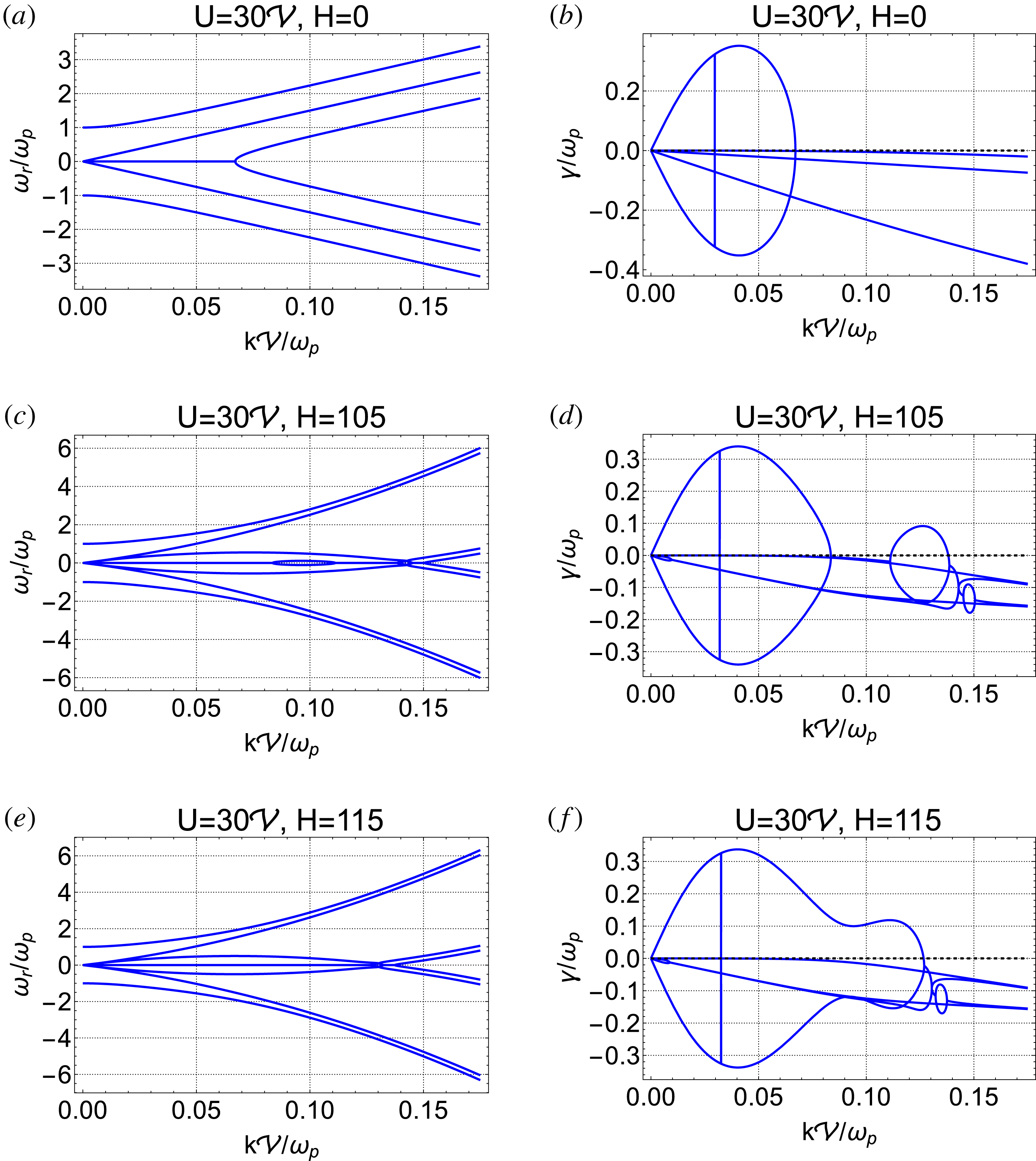
Exact dispersion relations for symmetrical counter-drifting inverse-quartic flat-top
 $\unicode[STIX]{x1D712}_{4}$
distribution functions (Case 1). The behaviour is generally similar to that of the Cauchy distributions as seen in figures 13 and 17, with the existence of a pair of new modes which interact with the unstable mode at the point where the second region of instability terminates (i.e.
 $k_{3}$
).

Exact dispersion relations for primary inverse-quartic flat-top
 $\unicode[STIX]{x1D712}_{4}$
distribution function population with low-density drifting beam with
 $n=1/100$
(Case 2). The behaviour is consistent with the general similarities with the dispersion relation of the squared Cauchy distribution in Case 1 and the one-population case.

Region of instability for counter-streaming inverse-quartic distributions with
 $H=0$
, (blue solid),
 $H=10$
(black dashed) and
 $H=30$
(orange dot-dashed). As in the squared Cauchy system, the second region of instability is seen to emerge for smaller
 $H$
than the Cauchy system. Aside from differing values of
 $U_{\text{crit}}$
, the figure is almost identical to the squared Cauchy instability region shown in figure 19.

5 Discussion
The phenomena studied in this paper overlap in part with other studies. delta-function and Cauchy distributions have been used to study quantum plasma instabilities by Haas et al. (Reference Haas, Bret and Shukla2009) and Haas et al. (Reference Haas, Manfredi and Goedert2001), respectively, while analysis of the two more complicated distribution functions (squared Cauchy and inverse quartic) in the context of quantum plasmas has not until now appeared in the literature, to the best of our knowledge. The dispersion relation derived by Haas et al. (Reference Haas, Bret and Shukla2009) agrees with that of this paper, including the existence of the second region of instability at larger wavenumbers
 $k$
. In Haas et al. (Reference Haas, Manfredi and Goedert2001) the solutions for the region of instability are in partial agreement with ours, but that paper does not explicitly solve for the dispersion relation and does not note the existence of the second region of instability, which we have shown is still present for the Cauchy distribution and its generalisations. Our paper is also relevant to the results in Bonitz et al. (Reference Bonitz, Binder, Scott, Koch and Kremp1993) in which streaming instabilities in degenerate Fermi–Dirac plasmas are considered, but no second region of instability is reported. The region of instability for this case is shown in figure 22.
The quantum longitudinal dielectric function used in this paper has been derived (Lindhard Reference Lindhard1954; Klimontovich & Silin Reference Klimontovich and Silin1960) under the assumptions of immobile ions, ideal non-interacting electrons, non-relativistic speeds, absence of a background magnetic field and spinless electrons. Despite these limitations, the resulting problem is rich in complexity and has revealed interesting new physics. However, these assumptions in principle may be relaxed in order to more obtain a more comprehensive understanding and extend the region of applicability. Several steps have already been taken to do this in the instance of single-population plasmas. The more realistic case of Fermi–Dirac electrons with an immobile ion background has been considered by Rightley & Uzdensky (Reference Rightley and Uzdensky2016). The introduction of ion motions through the inclusion of a classical ion susceptibility with arbitrarily degenerate quantum electrons has been carried out in the case by Melrose & Mushtaq (Reference Melrose and Mushtaq2010a ), under the assumptions of weak damping and long wavelength. The equation of motion for the Wigner function including an arbitrary magnetic field has been derived recently by Tyshetskiy et al. (Reference Tyshetskiy, Vladimirov and Kompaneets2011), and the dielectric tensor for a uniformly quantum plasma has been derived by other means by Canuto & Ventura (Reference Canuto and Ventura1972). Additionally, the filamentation instability in quantum plasmas has been analysed using a fluid approach by Bret (Reference Bret2007) and using a kinetic approach by Bret & Haas (Reference Bret and Haas2011). The quantum Weibel instability has been studied by Haas & Lazar (Reference Haas and Lazar2008) using a fluid approach, and a kinetic approach has been taken by Haas (Reference Haas2008). A framework for modelling waves in relativistic quantum plasmas has been derived by Melrose (Reference Melrose2013) and the quantum relativistic longitudinal dielectric function has been presented by Melrose & Mushtaq (Reference Melrose and Mushtaq2010a ), although only the non-relativistic limit is considered in the bulk of the work. Spin effects are of interest in sufficiently quantum plasmas, and their possibility has been considered in a quantum fluid or magnetohydrodynamic framework (Marklund & Brodin Reference Marklund and Brodin2007; Brodin & Marklund Reference Brodin and Marklund2008) but there has also been progress in spin kinetic theory (Marklund, Zamanian & Brodin Reference Marklund, Zamanian and Brodin2010; Andreev Reference Andreev2015, Reference Andreev2016; Iqbal & Andreev Reference Iqbal and Andreev2016; Andreev Reference Andreev2017). Certain kinetic and fluid spin models are reviewed by Brodin et al. (Reference Brodin, Marklund, Zamanian and Stefan2011). Nonlinear waves in quantum plasmas have mostly been studied as fluid phenomena (Shukla & Eliasson Reference Shukla and Eliasson2010), but the nonlinear regime of Landau damping has been investigated by Daligault (Reference Daligault2014), Brodin, Zamanian & Mendonca (Reference Brodin, Zamanian and Mendonca2015).
The results obtained in this paper are useful for the continued study of instabilities in quantum plasmas by building a knowledge base. Specifically, they provide a baseline for comparison of an in-progress detailed study of streaming instabilities in plasmas with arbitrarily degenerate Fermi–Dirac electrons employing numerical solutions of the dispersion relation. Additionally, further general insight into these phenomena can be gained by utilising the generalised Cauchy-type distribution functions mentioned in § 3.1. In this manner the influence of complex poles in the distribution function on the roots of the dielectric function can be systematically analysed. This is relevant because of the presence of branch cuts in the arbitrarily degenerate Fermi–Dirac distribution function, as discussed by Vladimirov & Tyshetskiy (Reference Vladimirov and Tyshetskiy2011).
Aside from the issue of obtaining a correct theoretical understanding of Landau damping and streaming instabilities in degenerate plasmas, the topic of quantum linear waves and instabilities is relevant to studies of warm dense matter, white dwarf interiors (Akbari-Moghanjoughi Reference Akbari-Moghanjoughi2013) and solid-state plasmas, in which the dielectric properties of the electrons are of importance. Furthermore, the quiescent X-ray emission of magnetars may be due to the dissipation of magnetospheric currents penetrating into the upper layers of the neutron star’s surface (Beloborodov & Thompson Reference Beloborodov and Thompson2007; Beloborodov Reference Beloborodov2009), where the current-carrying energetic electron–positron pairs deposit their energy into the layer by exciting Langmuir turbulence (Thompson & Beloborodov Reference Thompson and Beloborodov2005; Uzdensky & Rightley Reference Uzdensky and Rightley2014).
6 Conclusions
In summary, in this work we have used the established quantum longitudinal susceptibility to study the complex dispersion relation for electrostatic waves in plasmas consisting of one and two populations of electrons with uniform stationary ion background. We have considered four Wigner distribution functions that lend themselves to convenient analysis: the delta-function distribution, the Cauchy distribution, the squared Cauchy distribution and the inverse-quartic distribution. Other studies have established dispersion relations for instabilities in two-component plasmas with both components having either delta-function (Haas & Shukla Reference Haas and Shukla2009) or Cauchy (Haas et al. Reference Haas, Manfredi and Goedert2001) distributions, but have considered only the case of symmetrical counter-propagating electron populations with equal particle densities. This work extends these results by additionally considering the case of a primary electron population impinged upon by a delta-function beam of low density.
We have found that the normal mode structure in a given plasma becomes increasingly complex for more complicated distribution functions, but that for each distribution function considered, there is a normal plasmon mode, and a single unstable mode at small wavenumbers
 $k$
for two populations separated by sufficient drift velocity. However, unlike in the classical situation, there can exist a second region of instability for larger
 $k$
that is due entirely to quantum effects. This has been initially noted for the case of two counter-propagating cold beams by Haas et al. (Reference Haas, Bret and Shukla2009), and we have shown that this effect carries over to distribution functions with finite temperatures. Additionally, we have shown that the boundary of the region of instability at small
 $k$
for large drift velocity
 $U$
is affected by quantum effects at fifth order in
 ${\mathcal{V}}/U$
, where
 ${\mathcal{V}}$
is the thermal velocity. The results for the case with a cold beam penetrating a hot plasma with an analytically convenient distribution function are generally similar for the Cauchy, squared Cauchy, and inverse-quartic distribution functions. For each type of distribution function, the existence of one region of instability for small or zero quantum parameter
 $H$
, and of a second unstable window for sufficiently large
 $H$
, are preserved.
While our analysis accounts for the effects of quantum recoil, the analytically convenient distribution functions used in this paper do not account for quantum statistics. A more realistic description of quantum plasma instabilities would include a Fermi–Dirac (FD) background distribution function. The intent of this paper is to pave the way for studies of instabilities in FD plasmas, in which analytical results will be limited by the presence of branch cuts of the FD distribution function in complex-velocity space. For FD plasmas, it is therefore necessary to obtain the general dispersion relation using numerical methods, as has been performed for single-population plasmas in our previous work (Rightley & Uzdensky Reference Rightley and Uzdensky2016). This has been carried out in tandem with the present study, with results to be published in the near future. Ultimately, a complete understanding of Landau damping and streaming instabilities in degenerate electron plasmas will have applications to phenomena which are sensitive to the dielectric properties of the electrons in environments such as warm dense matter, dense astrophysical plasmas and solid-state plasmas. Furthermore, an understanding of nonlinear physics in these systems will be facilitated by a solid foundation in the linear theory. Finally, quantum effects introduce a rich complexity to the topic of linear waves and instabilities in plasmas, and have opened up new avenues of research in this direction.