During the 1920s Britain's rate of economic growth lagged behind that of many other countries in the world economy. Much of the historical literature has attempted to explain this outcome in terms of the macroeconomic policy regime resulting from the return to a fixed exchange rate at the prewar gold standard parity in 1925.1
Moggridge, British Monetary Policy; Broadberry, British Economy; and Temin, Lessons.
Despite some agreement on the magnitude of overvaluation in 1925 and a consensus that the overvaluation was greater in 1920, the absence of consistent data has resulted in the co-existence of a number of views that are clearly contradictory. For example, David Greasley and Les Oxley argue that the sterling real exchange rate became overvalued mainly during World War I.
2 Greasley and Oxley, “Discontinuities.”
Nicholas Dimsdale reports that the real effective exchange rate appreciated significantly over the period 1921–1925, whilst B. P. A. Andrews finds a real effective exchange rate peak in 1920, followed by a cycle of depreciation until 1922 and appreciation over 1922–1925.
3 Dimsdale, “British Monetary Policy.” Andrews, Exchange Rate Appreciation.
The absence of agreed data means that we cannot seriously evaluate how the exchange rate overvaluation affected aspects of the British economy during the 1920s.
The main study of Britain's real effective exchange rate during the 1920s is John Redmond's “The Sterling Overvaluation in 1925: A Multilateral Approach,” which evaluates the degree of overvaluation in 1925 relative to 1913 from a purchasing power parity perspective. There are four main problems with Redmond's study that we wish to address here. First, Redmond uses a variety of weights (derived from trade data for 1925, 1928, and 1929) and finds that the effective exchange rate indices are not sensitive to the weights used. However, the volatility of exchange rates and prices during the transwar period means that the choice of weights does matter over that period. To deal with this we work with trade weights from 1920 and 1925.4
We also considered 1913 and 1929 weights. However, the effect of large price and nominal exchange rate movements on the real effective exchange rate is likely to be better captured by using weights from the early 1920s.
Secondly, Redmond used arithmetic averaging to derive the effective exchange rate index. In light of modern conventional practice, we work with geometric averaging.
5 The use of geometric averaging also has the advantage that the choice of a reference base period is immaterial, as a given percentage change between any two dates has the same interpretation.
Thirdly, Redmond used consumer and wholesale price indices constructed by the League of Nations during the interwar period. There are some major discrepancies between the League of Nations consumer price data and more recent historical national price series, which reflect significant improvements in the construction of index numbers and more representative coverage and weighting systems for consumer price indices. We use more recent consumer price series to improve the reliability of the real effective exchange rate indices. Finally, although Redmond's country coverage is extensive, Germany is omitted from the effective exchange rate index. We show that the exclusion of Germany is not important for the period covered by Redmond (1924–1930) but is important to the time-profile of nominal and real exchange rate movements in the early 1920s.
6 The omission of Germany is also common to other work on Britain's effective exchange rate, including Andrews, Exchange Rate Appreciation; and Dimsdale, “British Monetary Policy.”
Although a number of studies have explicitly considered the pre-1924 period, improvements can be made to the existing indices. For example, Andrews reports an effective exchange rate against 11 of the major currencies, covering 11 countries until 1924 and 13 countries from 1925 (with the inclusion of Germany and Austria).7
Belgium, Canada, Czechoslovakia, France, India, Italy, Japan, Netherlands, Sweden, Switzerland, and the United States. In fact, Andrews (Exchange Rate Appreciation, pp. 392–402) notes that he was unable to find wholesale price data for Belgium, Czechoslovakia, and Switzerland for 1920. As a result the 1920 observation is an eight-country index.
Although this index has been used in discussions of the early 1920s the index is unsatisfactory in a number of ways.
8 Broadberry, British Economy.
First, the trade coverage is low, amounting to 49 percent of British trade in 1920 and an average of only 50 percent over the period 1920–1924.
9 Similar problems apply to Dimsdale's index based on an 11-country effective exchange rate using 1929 multilateral weights, excluding Germany. The countries selected by Dimsdale are Belgium, Canada, France, India (from 1921), Germany (from 1925), Italy, Japan, Netherlands, Switzerland, Sweden, and the United States.
Second, Andrews uses wholesale prices (mainly from League of Nations data) to derive a real effective exchange rate for this period. Given that consumer price indices display significant positive co-movement with GDP deflators it would be interesting to derive a consumer-price-based real exchange rate, relevant for analysing macroeconomic adjustment. Finally, the exclusion of Germany in the calculation produces a significant distortion to the time profile of the effective exchange rate index during the early 1920s.
NOMINAL EFFECTIVE EXCHANGE RATE IN THE 1920S
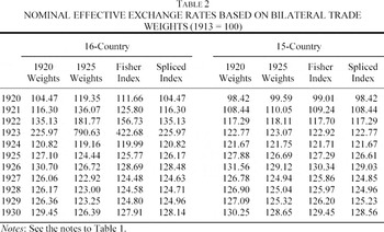
A number of nominal effective exchange rate (NEER) indices are constructed using bilateral trade weights for Britain's major trading partners and multilateral weights based on shares of world trade.10
The relative merits of bilateral and multilateral weights have been discussed extensively in the existing literature. For example, see Redmond “Sterling Overvaluation,” pp. 528–29. The multilateral weights used by the existing literature are taken from Maizels, Industrial Growth, chapter 8. These have the advantage of focusing on manufacturing exports but have the major disadvantage of being 1929 weights. In this study we have chosen to use shares of world trade, allowing us to derive weights relevant to the early 1920s. The sources for both sets of weights are reported in a longer version of this article available from the authors.
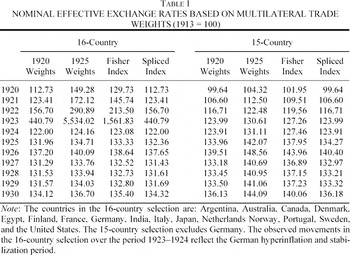
Exchange rates are expressed as the foreign price of domestic currency, with 1913 equal to 100. For the period 1920–1924 we use 1920 weights and for the period 1925–1930 we use 1925 weights. The series are spliced together in 1924 to create chain-indices for the NEER. To evaluate the sensitivity of results to the different methods that are used we also report the geometric average of the 1920 and 1925 weighted indices as a Fisher index number. To maintain comparability with the real effective exchange rate calculations reported later we calculated a NEER based on a comparable set of 16 countries.
11 Argentina, Australia, Canada, Denmark, Egypt, Finland, France, Germany, India, Italy, Japan, Netherlands Norway, Portugal, Sweden, and the United States. This group accounted for 68 percent of British trade in 1920 and 63 percent in 1925. Increasing the coverage to 21-country selection yields very similar magnitudes and patterns to the 16-country selection.
In order to make more direct comparisons with existing studies we also constructed a 15-country series, excluding Germany from the selection of countries.
The adoption of a floating exchange rate regime by Britain and many other countries after World War I resulted in a phase of nominal appreciation of the pound. The NEER reached unprecedented heights during 1923 (the observed movements over the period 1923–1924 reflect the German hyperinflation and stabilization period) and saw significant appreciation during the period 1919–1922. Clearly, the inclusion of Germany affects the level of nominal appreciation and, as a result, has to be considered when constructing the real exchange rate index. Andrews justifies the exclusion of Germany from existing effective exchange rate indices in the following terms:12
In fact, Austria stabilized in 1922.
… hyperinflation in Germany and Austria combined with extremely rapid depreciation of their exchange rates up to the end of 1923 makes their inclusion problematical. Moreover, the relevance of these exchange rates to the competitive position of the UK would be very limited. These currencies were frequently not used in international trade, and various countries developed different practices for alternative valuations of German and Austrian exports.
He notes that the League of Nations pointed out that in 1923 around 60–70 percent of German exports was paid for in foreign currency.13
Andrews, Exchange Rate Appreciation, pp. 45–46.
The decision to exclude Germany prior to 1924 clearly imposes a strong assumption about the role of the German currency in international trade. Although the League of Nations data suggest some care is needed in interpreting exchange rate movements in 1923, the problem is likely to be less in the early stages of German hyperinflation. Given the evidence that in this period German currency depreciation resulted in rapid export growth despite some slowing world income growth (particularly during the depression of 1920–1921) it seems inappropriate to exclude Germany from the effective exchange rate calculations of 1920–1922.
14 German exports (in constant prices) grew by 21 percent during 1920–1921 and by a further 38 percent during 1921–1922. The British trade data show that the share of Germany in British trade rose in every year during 1920–1923. Thus, the choice of 1920 weights to represent the period 1920–1924 is acting to moderate the extent of currency appreciation, implying that the spliced index offers a lower bound to the extent of overvaluation. Holtfrerich (German Inflation, pp. 279–300) provides further evidence on the importance of the German currency in international trade.
Even for 1923 it seems sensible not to exclude Germany; instead we provide a series of calculations to evaluate the sensitivity of the effective exchange rate to the exclusion of Germany.
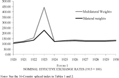
Tables 1 and 2 present NEER indices derived using multilateral and bilateral trade weights. Figure 1 illustrates the spliced indices. All the series yield similar patterns, suggesting that the NEER appreciated significantly over the period 1920–1922, appreciated even more so during 1922–1923, depreciated rapidly during 1923–1924, and appreciated again during 1925 and 1926. As would be expected, over the period 1920–1924 the magnitudes differ depending on the weighting system used. The general picture that emerges fits well with the financial and monetary history of the period, with the German hyperinflation and currency stabilization having a marked effect during the pre-1924 period.
FIGURE 1 NOMINAL EFFECTIVE EXCHANGE RATES (1913 = 100)
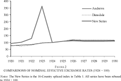
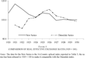
In Figure 2 the new NEER indices derived here are compared with the work of Andrews and Dimsdale by converting all the indices so that 1924 equals 100. The time-profile of exchange rate movements differs markedly within this period. The nominal appreciation of the sterling effective exchange rate was not smooth during the period 1920–1926, as implied in the calculations of Andrews and Dimsdale; instead, the period witnessed major shocks to the movement of the nominal effective exchange rate that are likely to have had implications for the time-profile of the real exchange rate, trade flows and other macroeconomic variables.15
The main reason for these differences is the exclusion of Germany. The 15-country effective exchange rate series reported in Table 1 (excluding Germany) displays very similar movements to the Andrews and Dimsdale series.
FIGURE 2 COMPARISONS OF NOMINAL EFFECTIVE EXCHANGE RATES (1924 = 100)
REAL EFFECTIVE EXCHANGE RATE
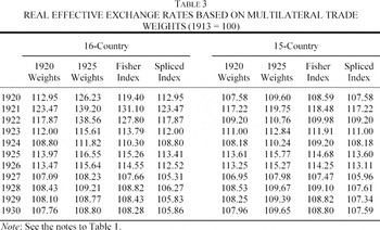
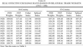
A number of real effective exchange rate (REER) indices are constructed using the same weights as were used for constructing the nominal effective exchange rate. Consumer prices have been used as deflators. Given the reliability of available price and exchange rate data for the United Kingdom and its main trading partners over the period 1920–1930 we produced a 16-country REER. Tables 3 and 4 present REER indices derived using multilateral and bilateral trade weights respectively. A very similar pattern is observed for the two series. The real exchange rate is above the 1913 PPP level in 1920 and appreciates further during 1920–1921. Although we observe a significant correction over the period 1921–1924, the real exchange rate remains over-valued in 1924 and appreciates further in 1924–1925.
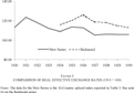
In light of the problems outlined previously, Figure 3 compares the new series with Redmond's index.16
To maintain comparability we used Redmond's retail price based measure of the British real effective rate based on multilateral trade weights for 16 countries and our multilateral series for 16 countries.
Redmond's series need to be revised in three significant ways: first, using consumer prices, the level of overvaluation in 1925 is much lower than that found by Redmond; second, the hike in the real exchange rate during 1926 is an artefact of the price data used by Redmond; and third, Redmond's indices display a large correction over 1926–1930 that is partly the result of serial correlation in the measurement error of the level of the real exchange rate in 1925 and 1926.
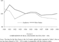
Figure 4 compares the new series with the Andrews index. To facilitate comparison the new series has been converted to the base level used by Andrews, 1924 equals 100. The two series depict a very different time-profile for the real exchange rate. As we have seen, Andrews's series fails to describe the nominal effective exchange rate movements during the period 1920–1924, and this has a clear effect on the movements of the real effective exchange rate. To facilitate comparison with Dimsdale's series we have converted our series to the base level used by Dimsdale, 1929 equals 100 (see
Figure 5).
FIGURE 3 COMPARISON OF REAL EFFECTIVE EXCHANGE RATES (1913 = 100)
FIGURE 4 COMPARISON OF REAL EXCHANGE RATES (1924 = 100)
FIGURE 5 COMPARISON OF REAL EFFECTIVE EXCHANGE RATES (1929 = 100)
Our new series follows a comparable path to Dimsdale's series during 1924–1930 but differs markedly during the pre-1924 period.
CONCLUSIONS AND IMPLICATIONS
The new data show that although the immediate run up to the return to gold during 1924–1925 resulted in an appreciation of the nominal and real effective exchange rates, the size of this shock was relatively minor compared to the movements before 1921.17
The 1924–1925 appreciation was partly the result of speculators pushing up the currency in the belief that the Act of Parliament suspending the gold standard was due to expire in 1925 and it was politically unlikely that the act would be extended beyond 1925. This resulted in a oneway bet for speculators, resulting in a Sterling appreciation (see Miller and Sutherland, “Speculative Anticipations”).
In terms of magnitudes, the main shock to the U.K. economy from exchange rate appreciation is to be found in the transwar period, not in 1925. In fact, the major correction of the real exchange rate after 1921 resulted in a short-term boost to British exports and the balance of trade.
The time profile of the new real exchange rate indices offers a way to reconcile some of the inconsistencies in the historical literature. Barry Eichengreen suggested that because British exports grew rapidly during 1920–1924, the overvalued exchange rate was not as important as traditionally assumed.18
Eichengreen, “Inter-War Economy.”
The evidence presented here suggests that we need to be careful in analyzing and decomposing both the
short-run and
long-run effects that can arise from exchange rate movements. Eichengreen's observation can be reconciled with the fact that during the years 1921–1924 exchange rate movements gave a significant
short-term boost to British exports; however, the large appreciation of the real EER observed over the transwar period may have had adverse long-term effects that need to be considered when evaluating the performance of the British interwar economy.
19 Solomou, Themes, suggests that the long-term movements of exports and imports in the 1920s are consistent with the idea that real exchange rate shocks resulted in trade hysteresis effects.
We find that the level of the real exchange rate was already high in 1920 (relative to the 1913 PPP level) and appreciated further in 1921. The initial level in 1920 suggests that Britain's exchange rate problems need to be seen as resulting from a sequence of adverse effects. First, the war period left an inflationary legacy needing adjustment. Secondly, a cluster of adverse nation-specific supply-side and demand-side shocks during 1919–1921 increased the required level of adjustment. The combination of supply-side shocks (mainly in the form of the hours of work reduction in 1919–1920) and demand-side shocks (in terms of the monetary policy stance to return to the 1913 gold parity) suggests that the problems faced by the British interwar economy are multi faceted.
Research for this article has been supported by a Research Grant from the ESRC (L138 25 1045). We would like to express our thanks to three anonymous referees of the JOURNAL, Cristiano Ristuccia, and Carl Holtfrerich for comments on an early version of this article. We would also like to thank Jan Klovland for providing us with price and exchange rate data on the Scandinavian economies. The usual disclaimer applies.