1. Introduction
Undulatory swimming, characterized by the generation of a travelling wave along the swimmer’s body or its propulsive cilia/fins, is one of the most widely adopted propulsion mechanisms across various length scales (Lauga & Powers Reference Lauga and Powers2009; Smits Reference Smits2019). This swimming mode is observed in a wide range of organisms, including microorganisms (e.g. Borrelia burgdorferi, Paramecium and Opalina), spermatozoa, millimetre-scale organisms (e.g. Caenorhabditis elegans, larva biting midges and ceratopogonid larvae), centimetre-scale worms (e.g. leeches), and high Reynolds number anguilliform swimmers (e.g. eels and marine snakes) and cartilaginous fishes (e.g. rays and skates). Understanding of the underlying physics of undulatory swimming is crucial for advancing our knowledge of biological locomotion and for designing biomimetic robots for different applications.
In his seminal work, Taylor (Reference Taylor1951) developed a model of a two-dimensional, infinite sheet propagating a transverse wave to study the swimming motion of microscopic organisms. Although the material points of the sheet undergo purely reciprocal motion, the combination of this motion with the propagation of the travelling wave over time results in non-reciprocal fluid movement, breaking time symmetry in Stokes flow, and enabling net movement at zero Reynolds number (
 $Re=0$
). Through a regular perturbation analysis of the small wave amplitude, Taylor showed that the propulsive velocity is
 $U=-c\varepsilon ^2/2$
, where
 $c$
is the wave speed, and
 $\varepsilon \ll 1$
is the wave amplitude normalized by the inverse of the wave number. The negative sign indicates that the swimming direction is opposite to the wave’s propagation. He later extended his analysis to a waving infinite cylinder, finding that it produces the same leading-order velocity as the waving sheet (Taylor Reference Taylor1952). Taylor’s swimming sheet model has since been applied widely to study undulatory motion under various conditions, including finite amplitude (Sauzade, Elfring & Lauga Reference Sauzade, Elfring and Lauga2011), near surfaces (Katz Reference Katz1974; Shack & Lardner Reference Shack and Lardner1974; Chrispell, Fauci & Shelley Reference Chrispell, Fauci and Shelley2013; Ives & Morozov Reference Ives and Morozov2017), in non-Newtonian fluids (Lauga Reference Lauga2007; Vélez-Cordero & Lauga Reference Vélez-Cordero and Lauga2013; Li & Ardekani Reference Li and Ardekani2015), in liquid crystals (Krieger et al. Reference Krieger, Spagnolie and Powers2014, Reference Krieger, Spagnolie and Powers2015; Soni Reference Soni2023), and in stratified fluids (Dandekar, Shaik & Ardekani Reference Dandekar, Shaik and Ardekani2019; Dandekar & Ardekani Reference Dandekar and Ardekani2020), as well as in studies of hydrodynamic interaction and synchronization (Elfring & Lauga Reference Elfring and Lauga2009, Reference Elfring and Lauga2011; Elfring, Pak & Lauga Reference Elfring, Pak and Lauga2010). All these works focus on the swimming motion in the low Reynolds number regime.
When considering fluid inertia, analysis of Taylor’s swimming sheet showed that at steady state, the swimming speed decreases monotonically with increasing
 $Re$
, approaching half the speed at
 $Re=0$
as the Reynolds number tends to infinity; see Reynolds (Reference Reynolds1965) and Tuck (Reference Tuck1968). Their studies also extended the model to include longitudinal waves, showing that at
 $Re=0$
, the swimming velocity has the same magnitude but an opposite direction compared to that of a transverse wave, and as
 $Re\to \infty$
, the speed approaches one and a half times the speed at
 $Re=0$
. Childress (Reference Childress2009) conducted a singular perturbation analysis of the swimming sheet in the limit of infinite Reynolds number, using matched asymptotic expansions for bulk and boundary layer regions. For a transverse wave, the analysis requires that the amplitude be small compared to the boundary layer thickness, and there is no solution in the inviscid limit due to the separation phenomenon. In contrast, the longitudinal wave does not require any additional assumption, and can be solved at arbitrary Reynolds numbers.
In the inviscid limit, undulatory swimming has also been studied through elongated-body theory and reactive force theory; for reviews, see Lighthill (Reference Lighthill1969) and Wu (Reference Wu2011). The swimming body is modelled as a finite, flexible ribbon plate oscillating in an inviscid fluid, resulting in a potential flow except for the vortex sheet generated on the body surface and free vortices shed from the trailing edge (Wu Reference Wu1961). Both theories predict that the mean thrust and mean power are positive when the swimming speed is lower than the wave speed. The hydrodynamic propulsive efficiency, defined as the ratio of effective power (mean thrust times mean velocity) to total power required for swimming, increases monotonically with the swimming speed (Lighthill Reference Lighthill1970; Wu Reference Wu1971b ). However, due to D’Alembert’s paradox of zero drag, the swimming speed can be estimated only by evaluating the swimmer’s viscous drag or by assessing the metabolic conversion of muscular power through oxygen consumption.
Most previous studies have focused on the steady motion of a waving sheet. However, transient motion and intermittent swimming are commonly observed in undulatory locomotion. The burst-and-coast swimming style, prevalent in many species of fish and other aquatic animals, is energetically more efficient than continuous undulatory swimming (Weihs Reference Weihs1974; Videler & Weihs Reference Videler and Weihs1982). At the microscopic scale, sperm cells of the sea urchin Tripneustes gratilla, when suspended in seawater with natural levels of
 $\mathrm{Ca}^{2+}$
, exhibit intermittent swimming, where flagellar beating is interrupted by irregular short quiescent periods (Gibbons & Gibbons Reference Gibbons and Gibbons1980). Similarly, C. elegans and several other nematode species display episodic swimming in liquid environments, characterized by regular alternations between active swimming and quiescence (Ghosh & Emmons Reference Ghosh and Emmons2008). Transient motion and rapid acceleration from rest are critical for swimmers during predator–prey interactions. For instance, Sagitta elegans utilizes prescribed undulatory kinematics to achieve rapid acceleration from rest (Jordan Reference Jordan1992). At high Reynolds numbers, the musky Esox employs two distinct strike strategies when attacking solitary prey: a typical start pattern, in which the fish accelerates by propagating a propulsive wave along its initially straight posture, and a more efficient pattern, where the body bends into a pre-strike S-shaped posture before initiating forward movement (Webb & Skadsen Reference Webb and Skadsen1980).
So far, there are limited studies on the transient motion of a waving sheet. Wu (Reference Wu1971a
) studied the motion of a two-dimensional flexible plate swimming at arbitrary unsteady speeds using linearized inviscid flow theory. At intermediate Reynolds numbers, Jordan (Reference Jordan1992) analysed the acceleration of S. elegans, and found that the swimmer generates much larger instantaneous hydrodynamic forces than the temporal average, highlighting the significance of unsteady effects in transient motion. Pak & Lauga (Reference Pak and Lauga2010) solved the unsteady Stokes equation for the transient motion of Taylor’s swimming sheet in the low Reynolds number regime. They derived explicit expressions for the swimming speed in the Laplace domain. The solutions in the time domain were derived analytically for massless sheets and longitudinal waves. For more complicated cases, numerical Laplace inversion is used to solve the speed evolution over time. Since flow convection is neglected in their analysis, the leading-order O(
 $\varepsilon$
) flow field affects the O(
 $\varepsilon ^2$
) field only through the velocity boundary condition. As we will demonstrate later, in the inertial regime, the O(
 $\varepsilon$
) field exerts two additional influences on the O(
 $\varepsilon ^2$
) swimming velocity due to flow convection and hydrodynamic force. Based on an unsteady squirmer model, Wang & Ardekani (Reference Wang and Ardekani2012) analytically studied the unsteady hydrodynamics of small organisms, such as Paramecium, which swims by generating a metachronal wave of cilia beating on its surface. Their analysis shows that unsteady inertia can significantly affect the velocity evolution for microswimmers with high cilia beating frequency, for which the product of Reynolds number and Strouhal number may be large. The Stouhal number is defined as
 $St=lU/T$
, where
 $1/T$
is the beating frequency, and
 $l$
and
 $U$
are the characteristic length and velocity of the swimmer. This condition
 $St\,Re\gt 1$
is compatible with Taylor’s waving sheet model, as its swimming speed is much smaller than the waving speed.
In this work, we investigate the transient motion of Taylor’s swimming sheet in the inertial regime, considering both transverse and longitudinal waves. The organization of this paper is as follows. Section 2 describes the mathematical model and governing equations. Section 3 discusses the procedures for the Laplace transform and asymptotic analysis of small wave amplitudes. Section 4 derives the analytical expression for the sheet velocity in the Laplace domain using the residue theorem. In § 5, the time history of the sheet velocity is calculated numerically in the time domain. Finally, conclusions are presented in § 6.
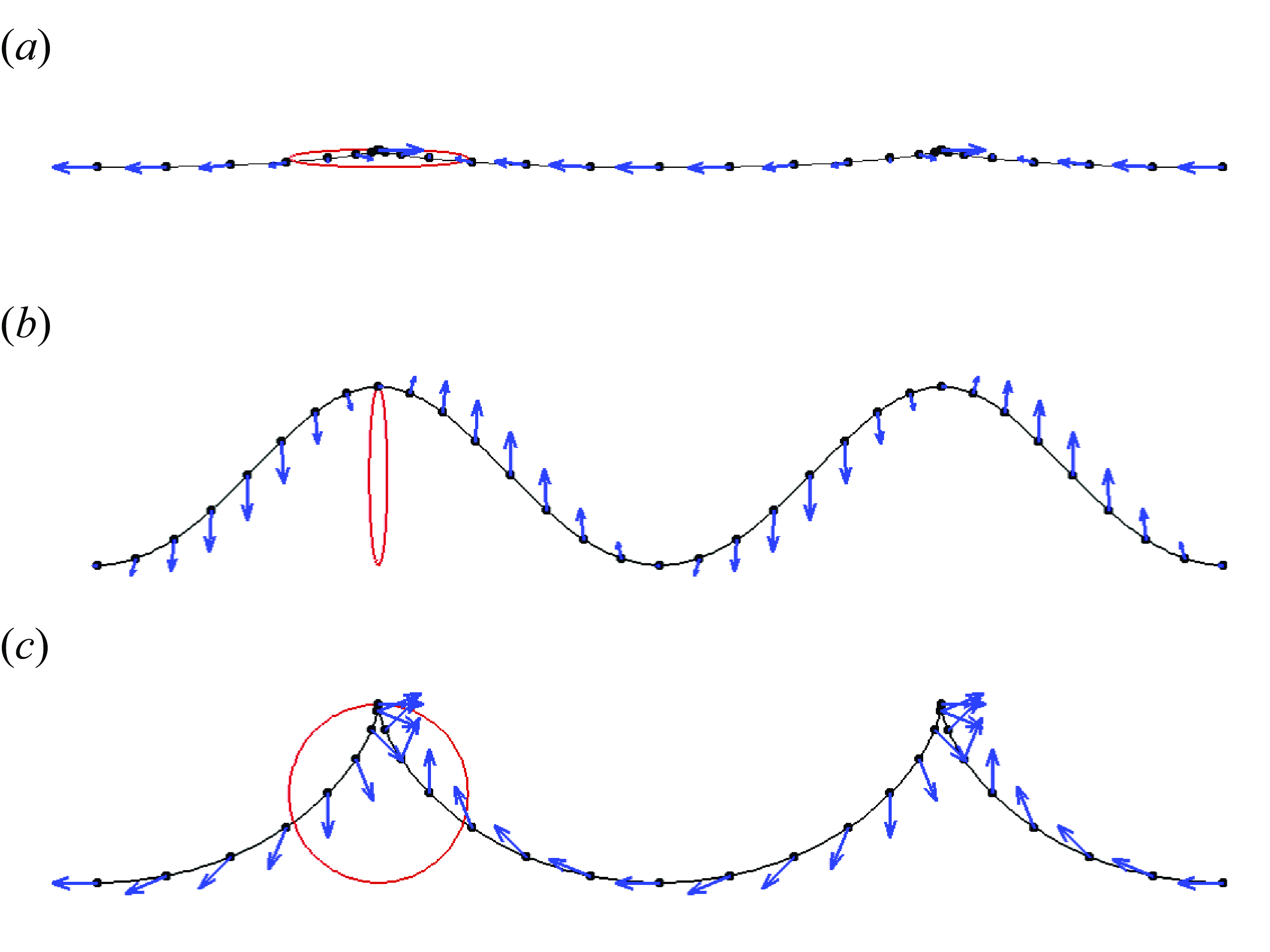
Schematic of the infinitely-long sheet of (a) longitudinal-dominant motion with
 $a=10b$
, (b) transverse-dominant motion with
 $a=0.1b$
, and (c) combined longitudinal and transverse motion with equal wave amplitudes
 $a=b$
and phase difference
 $\phi =0$
. Arrows indicate the instantaneous velocities on the sheet, while ellipses represent the trajectories of material points. The sheets are depicted with exaggerated amplitudes for clarity.

2. Swimmer model and governing equations
As shown in figure 1, we consider the swimming motion of an infinitely long, small-amplitude sheet in an incompressible fluid, driven by propagation of both longitudinal and transverse waves. In a non-inertial reference frame fixed on the sheet, the positions of the material points on the swimmer are
 \begin{align} x_s^*&=x^*+aA\left (\cos (kx^*-\omega t^*-\phi )\,f(t^*)+x^*_{0}(x^*)\,(1-f(t^*))\right ), \nonumber\\ y_s^*&=bA\left (\sin (kx^*-\omega t^*)\,f(t^*)+y^*_{0}(x^*)\,(1-f(t^*))\right ), \end{align}
where the dimensionless variables
 $a\geqslant 0$
and
 $b\geqslant 0$
represent the contributions of longitudinal and transverse motions, respectively,
 $A$
is the typical wave amplitude,
 $k$
is wavenumber,
 $\omega$
is frequency,
 $\phi$
is the phase difference between two motions,
 $x^*_{0}(x^*)$
and
 $y^*_{0}(x^*)$
represent the initial configurations of the sheet, and
 $f(t^*)$
is an arbitrary function of time that governs the acceleration of the swimmer, satisfying
 $f(t^*)=0$
for
 $t^*\leqslant 0$
, and
 $f(t^*)=1$
as
 $t^*\to \infty$
.
We non-dimensionalize the problem as follows:
 $1/k$
for length,
 $1/\omega$
for time,
 $\omega /k$
for velocity, and
 $\mu \omega$
for stress and pressure, where
 $\mu$
is the fluid viscosity. In complex functions, the dimensionless positions of the material points become
 \begin{align} x_s&=x+\varepsilon\, \delta x_s, \quad \delta x_s=a\mathrm{Re}\left (\mathrm{e}^{-\mathrm{i}(x-\phi )}\,f_e(t)+x_{0}(x)\,(1-f(t))\right ),\nonumber\\ y_s&=\varepsilon\, \delta y_s,\quad \delta y_s=-b\mathrm{Im}\left (\mathrm{e}^{-\mathrm{i}x}\,f_e(t)+y_{0}(x)\,(1-f(t))\right ), \end{align}
where
 $\mathrm{Re}(\cdot )$
and
 $\mathrm{Im}(\cdot )$
denote the real and imaginary parts, respectively,
 $\delta x_s$
and
 $\delta y_s$
are the displacements of material points on the sheet, and
 $f_e(t)=f(t)\,e^{it}$
is used for brevity. The dimensionless amplitude
 $\varepsilon =Ak\ll 1$
is the small parameter employed in the perturbation analysis. The initial position of the sheet can be expanded into a Fourier series:
 \begin{align} x_{0}=\sum _{n=1}^\infty A_n\mathrm{e}^{-\mathrm{i}(nx-\phi )}, \quad y_{0}=\sum _{n=1}^\infty B_n\mathrm{e}^{-\mathrm{i}nx}, \end{align}
where
 $A_n$
and
 $B_n$
are arbitrary complex constants. The corresponding velocity at the surface of the sheet is
 \begin{align} u_s&=\frac {\partial xs}{\partial t} =a\varepsilon \mathrm{Re}\left (\mathrm{e}^{-\mathrm{i}(x-\phi )}\,f^{\prime}_e(t)-x_{0}(x)\,f^{\prime}(t)\right ),\nonumber\\ v_s&=\frac {\partial ys}{\partial t} =-b\varepsilon \mathrm{Im}\left (\mathrm{e}^{-\mathrm{i}x}\,f^{\prime}_e(t)-y_{0}(x)\,f^{\prime}(t)\right ), \end{align}
where the prime denotes the time derivative,
 $f^{\prime}_e=(f^{\prime}+if)\,e^{it}$
. For the sheet’s initial configuration, we consider two scenarios: the swimmer starts from a fully relaxed state as a straight line, i.e.
 $A_n=B_n=0$
for all
 $n$
, or the swimmer starts with a body deformation that matches the subsequent waving motion, i.e.
 $A_1=B_1=1$
and
 $A_n=B_n=0$
for
 $n\geqslant 2$
. Both initial states, straight-line posture and pre-strike body deformation, are utilized by Esox when attacking prey (Webb & Skadsen Reference Webb and Skadsen1980). The time function governing the development of the propagating wave is
 \begin{align} f(t)=H(t)(1-e^{-t/T})^m, \end{align}
where
 $H(t)$
is the Heaviside step function. The characteristic time scale
 $T$
and the power index
 $m\geqslant 0$
determine the rate of wave development from the initial configuration. For the waving sheet starting from an initial straight-line state (
 $A_1=B_1=0$
),
 $m=0$
corresponds to an impulsive change in position and infinitely large sheet velocities,
 $m=1$
represents a continuous change in position with an impulsive change in velocity, and
 $m=2$
represents continuous changes in both position and velocity. For the sheet with initial body deformation (
 $A_1=B_1=1$
),
 $m=0$
reflects a continuous change in sheet position with an impulsive change in velocity, while
 $m=1$
represents continuous changes in both position and velocity. The cases of impulsive and exponential start have also been considered by Pak & Lauga (Reference Pak and Lauga2010) in studying the transient motion of a waving sheet at low Reynolds numbers. Alternative expressions, such as the inverse tangent function (Pak & Lauga Reference Pak and Lauga2010) or the error function (Jordan Reference Jordan1992), have been employed to model transient swimming. Nevertheless, it is reasonable to expect that these formulations would not affect the results qualitatively. In this work, we focus on the cases
 $m=0$
and 1.
The fluid flow generated by the sheet’s motion is governed by the two-dimensional incompressible Navier–Stokes equations. In terms of the streamfunction
 $\psi$
, the governing equation is expressed as
 \begin{equation} \frac {1}{Re}\nabla ^4\psi -\frac {\partial \nabla ^2\psi }{\partial t} =\frac {\partial \psi }{\partial y}\frac {\partial \nabla ^2\psi }{\partial x} -\frac {\partial \psi }{\partial x}\frac {\partial \nabla ^2\psi }{\partial y}, \end{equation}
where
 $Re=\rho \omega /\mu k^2$
is the Reynolds number, and
 $\rho$
is the fluid density. The fluid velocity and vorticity are determined by the streamfunction as
 $u=\partial \psi /\partial y,\ v=-\partial \psi /\partial x$
and
 $\omega =-\nabla ^2\psi$
, respectively. In contrast to the momentum equation, the above equation, which describes the evolution of vorticity in a two-dimensional field, is unaffected by the non-inertial forcing term.
The initial and boundary conditions are
 \begin{align} &\qquad\qquad\quad \psi |_{t=0}=0, \end{align}
 \begin{align} & \frac {\partial \psi }{\partial y}\left|_{(x_s, y_s)}=u_s, \quad \frac {\partial \psi }{\partial x}\right|_{(x_s, y_s)}=-v_s, \end{align}
 \begin{align} & \frac {\partial \psi }{\partial y}\left|_{y\to \infty }=-U(t), \quad \frac {\partial \psi }{\partial x}\right|_{y\to \infty }=0, \end{align}
where
 $U(t)$
is the swimming velocity of the sheet, determined by Newton’s second law,
 \begin{equation} Re\,M\,\frac {{\rm d}U}{{\rm d}t}=F_x, \end{equation}
where
 $M=hk\rho _s/\rho$
is the dimensionless mass of the sheet per unit length, with
 $h$
representing the half-thickness of the sheet, and
 $\rho _s$
and
 $\rho$
the densities of the sheet and fluid. The
 $x$
-averaged hydrodynamic force on the swimmer along the swimming direction is given by
 \begin{align} F_x&=\frac {1}{2\unicode{x03C0} }\int _0^{2\unicode{x03C0} }\left ((-p+\tau _{xx})n_x+\tau _{xy}n_y\right )|_{(x_s, y_s)}\sqrt {\left (\frac {\partial x_s}{\partial x}\right )^2+\left (\frac {\partial y_s}{\partial x}\right )^2}{\rm d}x \nonumber\\ &=\left.\left \langle -(-p+\tau _{xx})\frac {\partial y_s}{\partial x}+\tau _{xy}\frac {\partial x_s}{\partial x}\right \rangle \right|_{(x_s, y_s)}, \end{align}
where
 $\langle \cdot \rangle = {1}/{2\unicode{x03C0} }\int _0^{2\unicode{x03C0} }(\cdot )\,{\rm d}x$
denotes the
 $x$
-average. Here,
 $p$
,
 $\tau _{xx}$
and
 $\tau _{xy}$
represent the pressure and the two components of the viscous stress, while
 $n_x$
and
 $n_y$
are the
 $x$
- and
 $y$
-components of the unit normal vector on the sheet.
The three key dimensionless parameters,
 $1/T$
,
 $Re$
and
 $M$
, represent the contributions of unsteady inertia, convective fluid inertia and swimmer inertia, respectively. In our study, the acceleration rate
 $1/T$
is equivalent to the Strouhal number defined in Wang & Ardekani (Reference Wang and Ardekani2012). Unsteady inertia becomes significant for microswimmers when the production of Strouhal number and Reynolds number exceeds unity, as observed in organisms such
as Paramecium, where
 $1/T\sim 20$
and
 $Re\sim 0.1$
(Wang & Ardekani Reference Wang and Ardekani2012). At mesoscales, both swimmer and fluid inertia can be non-negligible. For example, some free-living marine nematodes, such as those in the families Ironidae and Thoracostomopsidae, have body length
 $5{-}10$
mm, diameter
 $0.1$
mm, and swimming speed
 $0.5\ \mathrm{mm}\ \mathrm{s}^{-1}$
(Smol & Coomans Reference Smol and Coomans2006), resulting in a swimming Reynolds number
 $Re\sim 2{-}5$
and dimensionless mass
 $M\sim 0.1$
. For even larger swimmers, such as S. elegans with body length
 $\sim 2$
cm, diameter
 $\sim 2$
mm and speed
 $\sim 6\ \mathrm{cm}\ \mathrm{s}^{-1}$
(Jordan Reference Jordan1992), and leeches with body length
 $\sim 10$
cm, diameter
 $\sim 1$
cm and speed
 $\sim 4\ \mathrm{cm}\ \mathrm{s}^{-1}$
, the corresponding Reynolds number is
 $Re\sim 10^3$
, and the dimensionless mass is
 $M\sim 0.1$
(Taylor Reference Taylor1952).
3. Asymptotic analysis for small wave amplitude
We perform regular perturbation expansions to solve (2.6). The streamfunction and the swimming velocity of the sheet are expressed as
 \begin{equation} \psi =\varepsilon \psi _1+\varepsilon ^2\psi _2+\cdots, \quad U=\varepsilon U_1+\varepsilon ^2U_2+\cdots, \end{equation}
where
 $\varepsilon \ll 1$
is the characteristic amplitude in dimensionless form. We substitute these expansions into (2.6), (2.7) and (2.9), then apply the Laplace transform as
 \begin{equation} \tilde {\psi }(x,y,s)=\mathcal L(\psi (x,y,t))=\int _0^\infty \psi (x,y,t)\,e^{-st}\,{\rm d}t, \end{equation}
where
 $\mathcal L(\cdot )$
represents the Laplace transform, a tilde indicates a transformed quantity, and
 $s$
is the Laplace variable. Unless otherwise specified, the transformed quantities are considered functions of
 $s$
.
We solve the O(
 $\varepsilon$
) and O(
 $\varepsilon ^2$
) equations sequentially. In the Laplace domain, the O(
 $\varepsilon$
) equation and the boundary conditions under a domain perturbation reduce to
 \begin{align} &\qquad\qquad\qquad\qquad \frac {1}{Re}\,\nabla ^4\tilde {\psi }_1-s\,\nabla ^2\tilde {\psi }_1=0, \end{align}
 \begin{align} & \left.\frac {\partial \tilde {\psi }_1}{\partial y}\right|_{y=0}=as\mathrm{Re} \left (\tilde f_e(s)\,\mathrm{e}^{-\mathrm{i}(x-\phi )}-\tilde f(s)\sum _{n=1}^\infty A_n\, \mathrm{e}^{-\mathrm{i}(nx-\phi )}\right ), \end{align}
 \begin{align} &\qquad \left.\frac {\partial \tilde {\psi }_1}{\partial x}\right|_{y=0}=bs\mathrm{Im} \left(\tilde f_e(s)\,\mathrm{e}^{-\mathrm{i}x}-\tilde f(s)\sum _{n=1}^\infty B_n\, \mathrm{e}^{-\mathrm{i}nx}\right), \end{align}
 \begin{align} &\qquad\qquad\quad \left.\frac {\partial \tilde {\psi }_1}{\partial y}\right|_{y\to \infty }=-\tilde {U}_1(t),\quad \frac {\partial \tilde {\psi }_1}{\partial x}|_{y\to \infty }=0, \end{align}
where the prefactor
 $s$
in the equations arises from the time derivative. Since the convection term is not involved, the above equation describes the effects of unsteady inertia at leading order. For
 $f(t)=H(t)(1-e^{-t/T})^m$
and
 $f_e(t)=f(t)\,e^{it}$
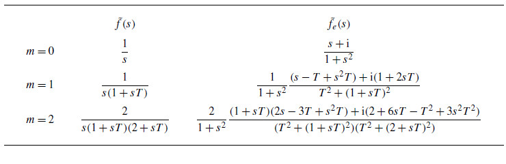
, the Laplace transforms are
 \begin{equation} \tilde f(s)=\frac {T\,\Gamma (m+1)\,\Gamma (sT)}{\Gamma (m+1+sT)},\quad \tilde f_e(s)=\frac {T\,\Gamma (m+1)\,\Gamma ((s-i)T)}{\Gamma (m+1+(s-i)T)}, \end{equation}
where
 $\Gamma (\cdot )$
is the gamma function. For integer values
 $m=0, 1, 2$
, the values of
 $\tilde f(s)$
and
 $\tilde f_e(s)$
are listed in table 1.
The values of
 $\tilde f(s)$
and
 $\tilde f_e(s)$
for different choices of the power index
 $m$
in the time function.

The solution that satisfies (3.3) is found to be
 \begin{align} &\tilde {\psi }_1(s)=s\mathrm{Re}\left(\big(a\,\mathrm{e}^{-\mathrm{i}(x-\phi )}+b\,\mathrm{e}^{-\mathrm{i}x}\big)\,\tilde f_e(s)\, \frac {e^{-y}-e^{-\sqrt {1+s\, Re}\,y}}{\sqrt {1+s\, Re}-1}+b\,\tilde f_e(s)\,e^{-(ix+y)}\right)\nonumber\\ &\!\!\quad{}-s\,\tilde f(s)\sum _{n=1}^\infty \mathrm{Re}\left(\big(aA_n\,\mathrm{e}^{-\mathrm{i}(nx-\phi )}\!+\!bB_n\,\mathrm{e}^{-\mathrm{i}nx}\big)\,\frac {e^{-ny}-e^{-\sqrt {n^2+s\, Re}\,y}}{\sqrt {n^2+s\, Re}-n} \!+\!\frac {b}{n}B_n\,e^{-n(ix+y)}\right)\nonumber\\ &\!\!\quad{}+\tilde {U}_1\left(\frac {e^{-\sqrt {s\,Re}\,y}}{\sqrt {s\,Re}}+y\right). \end{align}
The O(
 $\varepsilon$
) dynamical condition (2.8) for sheet swimming simplifies to
 \begin{equation} Re\,M\,\frac {dU_1}{dt}=\langle \tau _{1xy}|_{y=0}\rangle =\frac {1}{2\unicode{x03C0} }\int _0^{2\unicode{x03C0} }\left.\frac {\partial u_1}{\partial y}\right|_{y=0}\,{\rm d}x. \end{equation}
Note that the
 ${\partial v_1}/{\partial x}$
term in
 $\tau _{1xy}$
vanishes after taking the
 $x$
-average. In the Laplace domain, the dynamical condition becomes
 \begin{equation} Re\,Ms\tilde {U}_1=\frac {1}{2\unicode{x03C0} }\int _0^{2\unicode{x03C0} }\left.\frac {\partial ^2\tilde {\psi }_1}{\partial y^2}\right|_{y=0}\,{\rm d}x=\sqrt {s\,Re}\,\tilde {U}_1. \end{equation}
This leads to
 $\tilde {U}_1=0$
and therefore
 $U_1=0$
, indicating that there is no swimming motion at order
 $\varepsilon$
, as expected.
In the time domain, the O(
 $\varepsilon$
) streamfunction can be solved as
 \begin{equation} \begin{aligned} \psi _1(t)&=\mathrm{Re}\left (\big(a\,\mathrm{e}^{-\mathrm{i}(x-\phi )}+b\,\mathrm{e}^{-\mathrm{i}x}\big) f^{\prime}_e*G_1 +bf^{\prime}_e\,e^{-(ix+y)}\right )\\ &\quad{}-\sum _{n=1}^\infty \mathrm{Re}\left (aA_n\,\mathrm{e}^{-\mathrm{i}(nx-\phi )}+bB_n\,\mathrm{e}^{-\mathrm{i}nx}\right )f^{\prime}*G_n -f^{\prime}\sum _{n=1}^\infty \mathrm{Re}\left(\frac {b}{n}B_n\,e^{-n(ix+y)}\right), \end{aligned} \end{equation}
where
 \begin{align} G_n(t)&=\mathcal L^{-1}\left (\frac {e^{-ny}-e^{-\sqrt {n^2+Re\,s}\,y}}{\sqrt {n^2+Re\,s}-n}\right )\nonumber\\ &=\frac {e^{-ny}}{\sqrt {\unicode{x03C0}\, Re\,t}} \left (\exp\left({-\frac {n^2t}{Re}}\right) -\exp\left({-\frac {(2nt-Re\, y)^2}{4\,Re\,t}}\right)\right ) \nonumber\\&\quad +\frac {n\,e^{-ny}}{Re}\left (\mathrm{erf}\left(\sqrt {\frac {n^2t}{Re}}\right) -\mathrm{erf}\left(\frac {2nt-Re\, y}{2\sqrt {Re\,t}}\right)\right ), \end{align}
for
 $n=1,2,3,\ldots$
. Here, the symbol
 $*$
represents the time convolution, e.g.
 $f_1(t)*f_2(t)=\int _0^t f_1(t-\tau )\,f_2(\tau )\,{\rm d}\tau$
.
For the O(
 $\varepsilon ^2$
) terms, we solve for the
 $x$
-averaged equation for
 $\tilde \psi _2$
as follows:
 \begin{align} & \frac {1}{Re}\frac {\partial ^4\langle \tilde \psi _2\rangle }{\partial y^4} -s\frac {\partial ^2\langle \tilde \psi _2\rangle }{\partial y^2}=\tilde C_1^s(y), \quad \tilde C_1^s(y)=\mathcal L\left(\left\langle \frac {\partial \psi _1}{\partial y}\frac {\partial \nabla ^2\psi _1}{\partial x} -\frac {\partial \psi _1}{\partial x}\frac {\partial \nabla ^2\psi _1}{\partial y}\right\rangle \right), \end{align}
 \begin{align} &\qquad\quad \left.\frac {\partial \langle \tilde \psi _2\rangle }{\partial y}\right|_{y=0} =-\tilde U_1^s, \quad \tilde U_1^s=\mathcal L\left( \left.\left\langle \frac {\partial ^2\psi _1}{\partial x\,\partial y}\delta x_s +\frac {\partial ^2\psi _1}{\partial y^2}\delta y_s\right\rangle \right|_{y=0}\right), \end{align}
 \begin{align} &\qquad\qquad\qquad\qquad\qquad \left.\frac {\partial \langle \tilde \psi _2\rangle }{\partial y}\right|_{y\to \infty }=-\tilde U_2, \end{align}
where
 $\tilde C_1^s$
denotes the flow convection induced by the O(
 $\varepsilon$
) velocity field, and
 $\tilde U_1^s$
represents the ‘slip’ velocity on the sheet surface caused by the O(
 $\varepsilon$
) velocity.
For the dynamical condition, the O(
 $\varepsilon ^2$
)
 $x$
-average hydrodynamic force in the physical domain is
 \begin{equation} F_{2x}=\left.\left \langle \tau _{2xy}-(-p_1+\tau _{1xx})\frac {\partial \delta y_s}{\partial x}+\tau _{1xy}\frac {\partial \delta x_s}{\partial x}+\frac {\partial \tau _{1xy}}{\partial x}\delta x_s+\frac {\partial \tau _{1xy}}{\partial y}\delta y_s\right \rangle \right|_{y=0}, \end{equation}
where the sheet displacements
 $\delta x_s$
and
 $\delta y_s$
are defined in (2.2). On the right-hand side, the first term represents the O(
 $\varepsilon ^2$
) stress contribution, the second and third terms account for the O(
 $\varepsilon$
) stress contributions related to the orientation of the unit normal vector on the sheet surface, and the last two terms represent the O(
 $\varepsilon$
) stress contributions due to the displacement of the sheet from its equilibrium position at
 $x_s=x$
and
 $y_s=0$
. This equation can be simplified further. The third and fourth terms yield a zero net contribution when averaged over
 $x$
. By combining the second and last terms after partial integration, and applying the Navier–Stokes equation for
 $u_1$
, (3.11) becomes
 \begin{equation} F_{2x}=\left.\left \langle \tau _{2xy}+Re\,\frac {\partial ^2\psi _1}{\partial t\,\partial y}\,\delta y_s\right \rangle \right|_{y=0}. \end{equation}
Therefore, in the Laplace domain, the O(
 $\varepsilon ^2$
) dynamical condition for sheet swimming becomes
 \begin{equation} M\,Re\,s\tilde U_2=\left.\frac {\partial ^2\langle \tilde \psi _2\rangle }{\partial y^2}\right|_{y=0} +Re\,\tilde F_{1x}^s, \quad \tilde F_{1x}^s=\mathcal L\left (\left.\left\langle \frac {\partial ^2\psi _1}{\partial t\,\partial y}\delta y_s\right\rangle \right|_{y=0}\right ), \end{equation}
where the force contribution due to the O(
 $\varepsilon$
) flow field vanishes at
 $Re=0$
or for a pure longitudinal wave (
 $b=0$
). As will be demonstrated later, this term exists only for combined waves (
 $a\neq 0$
and
 $b\neq 0$
). Similar to
 $\tilde U_1^s$
, the forcing term
 $\tilde F_{1x}^s$
represents only the effects of unsteady inertia.
4. Sheet velocity in the Laplace domain
To solve (3.10) and (3.13), we first address the terms
 $\tilde C_1^s$
,
 $\tilde U_1^s$
and
 $\tilde F_{1x}^s$
on the right-hand side. The Laplace transform of the product of two functions can be transformed into the convolution of their respective Laplace transforms; for instance, the velocity
 $\tilde U_1^s$
in (3.10b
) can be written as
 \begin{equation} \begin{aligned} \tilde U_1^s=\frac {1}{2\unicode{x03C0} i} \int _{\alpha -i\infty }^{\alpha +i\infty }\underbrace {\left.\left \langle \frac {\partial ^2\tilde \psi _1(z)}{\partial x\,\partial y}\,\widetilde{\,\delta x\,}_s\,(s-z) +\frac {\partial ^2\tilde \psi _1(z)}{\partial y^2}\,\widetilde{\,\delta y\,}_s\,(s-z)\right \rangle \right|_{y=0}}_{u_1^s}\,{\rm d}z, \end{aligned} \end{equation}
where
 $\alpha$
is an arbitrary constant satisfying
 $0\lt \alpha \lt s$
for convergence. The ‘slip’ velocity represents the leading-order contribution of the unsteady inertia effect. Substituting (2.2) and (3.5), the integrand in the above equation is solved for the case
 $\mathcal I(A_1)=\mathcal I(B_1)=0$
and
 $A_n=B_n=0$
for
 $n\geqslant 2$
:
 \begin{equation} \begin{aligned} & u_1^s=\frac {a^2z}{2}\mathcal I\left (A_1\,\tilde f_e(z)\left(\frac {1}{s-z}-\tilde f(s-z)\right) +\tilde f_e^\dagger (s-z)\,\left(\tilde f_e(z)-A_1\,\tilde f(z)\right)\right )\\ &\quad{}+\frac {b^2z}{2}\mathcal I\left (\! B_1\,\tilde f_{R}(z)\left(\frac {1}{s-z}-\tilde f(s-z)\right) +\tilde f_e^\dagger (s-z)\,\left(\tilde f_R(z)-B_1\sqrt {1+Re\,z}\,\tilde f(z)\right)\!\right )\!, \end{aligned} \end{equation}
for which
 $z$
is temporally viewed as real,
 $\tilde f_e^\dagger$
is the complex conjugate of
 $\tilde f_e$
, and
 \begin{equation} \tilde f_{R}(z)=\sqrt {1+Re\,z}\,\tilde f_e(z)+\frac {a}{b}\left(1+\sqrt {1+Re\,z}\right)(\tilde f_e(z)-A_1\,\tilde f(z))\,e^{i\phi }. \end{equation}
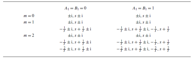
Positions of the poles in complex plane for equation (4.2) with different values of
 $A_1, B_1$
and
 $m$
.


The integral in (4.1) is performed along a vertical line
 $\mathcal R(z)=\alpha$
, which must lie entirely within the region of convergence of
 $\widetilde {\delta x}_s(s-z),\ \widetilde{\,\delta y\,}_s(s-z)$
and
 $\tilde \psi _1(z)$
(Doetsch Reference Doetsch2012). To evaluate this complex integral, we apply Cauchy’s residue theorem. Its integrand contains poles inherited from
 $\tilde f$
and
 $\tilde f_e$
, as well as a branch point at
 $s=-1/Re$
, caused by the square root term in
 $\tilde \psi _1$
. Table 2 lists the locations of the poles for (4.2) with different values of
 $A_1, B_1$
and
 $m$
. Figure 2(a) illustrates the complete set of poles and the branch cut in the complex plane for this function. As
 $m$
increases, new poles are introduced at
 $z=s+ ({m}/{T})+li$
and
 $z=- ({m}/{T})+li$
, where
 $l=-1, 0, 1$
. The pair of poles on the real axis (
 $l=0$
) results from the condition of the initial position (
 $A_1=B_1=1$
) of the waving sheet. The integration is performed along a vertical line within the strip region
 $0\lt \mathcal R(z)\lt s$
to ensure convergence. This integral equals the integral along an infinitely large half-circle of radius
 $R$
, minus the sum of the residues inside the closed loop. Consequently, the term on the right-hand side of (3.10b
) in real form is found to be, for
 $m=0$
,
 \begin{equation} \begin{aligned} \tilde U_1^s&=\frac {a^2-b^2(r_1^++sr_1^-)-ab\left ((1+r_1^++sr_1^-)\cos \phi +(s(1+r_1^+)-r_1^-)\sin \phi \right )}{2s}\\ &\quad{}+\frac {B_1b^2r_1^-+A_1ab\left (r_1^-\cos \phi +(1+r_1^+)\sin \phi \right )}{2} +\left(\frac {1}{4}+\frac {\sqrt {Re\, R}}{\sqrt {2}\,\unicode{x03C0} }\right)\!(1-A_1)ab\sin \phi, \end{aligned} \end{equation}
where the following substitutions are made for brevity:
 \begin{align} &r_1^\pm =\frac {1}{\sqrt {2}}\sqrt {\left ((1+Re\ s)^2+Re^2\right )^{1/2}\pm (1+Re\ s)},\nonumber\\ &r_2^\pm =\frac {1}{\sqrt {2}}\sqrt {\left (r_T^4+Re^2\right )^{1/2}\pm r_T^2},\quad r_T=\sqrt {1+Re\,(s+T^{-1})}. \end{align}
The last term in (4.4) results from the integral along the half-circle at infinity, and diverges as
 $\sqrt {R}$
for a coupled longitudinal and transverse waving motion when
 $A_1\neq 1$
, where
 $R$
is the radius of the half-circle.
For
 $m=1$
, the integral along the infinite half-circle vanishes, and the velocity
 $\tilde U_1^s$
is
 \begin{equation} \begin{aligned} \tilde U_1^s&=\frac {2a^2-b^2T^A_1-ab((T^A_1+2)\cos \phi +T^A_2\sin \phi )}{2s(1+Ts)(2+Ts)} +\frac {A_1B_1ab}{2(2+Ts)}(r_T+1)\sin \phi \\ &\quad{}+\frac {A_1a^2T_2-B_1b^2r_TT_1-B_1ab(T_1\cos \phi +T_3\sin \phi )(r_T+1)} {2(T^2+(1+Ts)^2)(T^2+(2+Ts)^2)}\\ &\quad{}+\frac {B_1b^2T^B_1-A_1ab\,Re\left (g_1(1-r_1^+, r_1^-)\cos \phi -g_1(r_1^-, r_1^+-1)\sin \phi \right )} {2(T^2+(1+Ts)^2)(r_1^{-2}+(1-r_1^+)^2)}\\ &\quad{}-\frac {B_1b^2T^B_2-A_1ab\,Re\left (g_2(1-r_2^+, r_2^-)\cos \phi -g_2(r_2^-, r_2^+-1)\sin \phi \right )} {2(T^2+(2+Ts)^2)(r_2^{-2}+(1-r_2^+)^2)}, \end{aligned} \end{equation}
for which the coefficients are
 \begin{align} &T_1=T(1+Ts)(3+2Ts),\quad T_2=T(2+Ts)(3+2Ts),\nonumber\\ &T_3=(1+Ts)^2(2+Ts)-T^2(1+Ts),\nonumber\\ &T^A_1=(2+Ts)(r_1^+ +sr_1^-) -Ts(r_2^+ +sr_2^-) -sr_2^-,\nonumber\\ &T^A_2=(2+Ts)(sr_1^+ -r_1^-) -Ts(sr_2^+ -r_2^-) -s(r_2^+-1),\nonumber\\ &T^B_1=\left ((1-r_1^+)^2+r_1^{-2}\right )T-Re\,\left (1-r_1^++(s(1+Ts)+T)r_1^-\right ),\nonumber\\ &T^B_2=\left ((1-r_2^+)^2+r_2^{-2}\right )T-Re\,\left (1-r_2^++((s+T^{-1})(2+Ts)+T)r_2^-\right ), \end{align}
and the two functions
 $g_1(x, y)$
and
 $g_2(x, y)$
are defined as
 \begin{equation} g_1(x, y)=x+(s(1+Ts)+T)y, \quad g_2(x, y)=x+((s+T^{-1})(2+Ts)+T)y. \end{equation}
Similarly, we can calculate the force term
 $\tilde F_{1x}^s$
in (3.13). It turns out that its integrand has exactly the same poles as that of
 $\tilde U_1^s$
, but it has no branch points. Therefore, the integral along the vertical line can be calculated using either the right or left half-circle loops. For
 $m=0$
,
 \begin{equation} \tilde F_{1x}^s=\frac {ab\left ((2-A_1)s\cos \phi -(2-(1-A_1)s^2)\sin \phi \right )}{4s}- \frac {(1-A_1)abR\sin \phi }{2\unicode{x03C0} }, \end{equation}
which diverges linearly as the radius
 $R$
of the half-circle approaches infinity.
For
 $m=1$
, the force is
 \begin{equation} \begin{aligned} \tilde F_{1x}^s&=ab\frac {2Ts\cos \phi -(2T+s)\sin \phi }{2Ts(1+Ts)(2+Ts)} +\frac {A_1ab}{2T}\frac {(1+Ts)^{-1}(-T_1\cos \phi +T_3\sin \phi )}{(T^2+(1+Ts)^2)(T^2+(2+Ts)^2)}\\ &\quad{}+\frac {B_1ab}{2T}\left (\frac {(1+Ts)(T_1\cos \phi +T_3\sin \phi )}{(T^2+(1+Ts)^2)(T^2+(2+Ts)^2)}-\frac {\sin \phi }{2}\right )-\frac {A_1B_1abs\sin \phi }{4(2+Ts)}, \end{aligned} \end{equation}
where
 $T_1$
and
 $T_3$
are defined in (4.7). The result shows that only a sheet exhibiting both longitudinal and transverse waves contributes to the force from the O(
 $\varepsilon$
) flow to the O(
 $\varepsilon ^2$
) sheet velocity.
For the convection term, rather than calculating
 $\tilde C_1^s$
, we directly solve (3.10a
) to obtain the
 $x$
-averaged velocity field:
 \begin{equation} \begin{aligned} \frac {\partial \langle \tilde \psi _2\rangle }{\partial y} &=\frac {\sqrt {Re}}{\sqrt {s}}\int _0^y\!\int _0^{y^{\prime}}\sinh (\sqrt {Re\,s}\,(y^{\prime}-y^{\prime\prime}))\,\tilde C_1^s(y^{\prime\prime})\,{\rm d}y^{\prime\prime}\,{\rm d}y^{\prime}+C_1\,e^{-\sqrt {Re\,s}\,y}\\&\quad +C_2\,e^{\sqrt {Re\,s}\,y}+C_3. \end{aligned} \end{equation}
Using the boundary and dynamical conditions (3.10b
), (3.10c
) and (3.13), we can solve for the constants
 $C_1, C_2, C_3$
and determine the swimming velocity of the sheet in the Laplace domain. The order of integration for the Laplace transform and the
 $x$
-average can be freely interchanged with the integrals over
 $y^{\prime}$
and
 $y^{\prime\prime}$
since their intervals are independent. Similar to the terms
 $\tilde U_1^s$
and
 $\tilde F_{1x}^s$
, the term
 $\tilde C_1^s$
can also be expressed as a convolution integral. After rearranging the integrals and performing the integrations over
 $x$
,
 $y^{\prime}$
and
 $y^{\prime\prime}$
, the sheet velocity in the Laplace space can be solved:
 \begin{equation} \begin{aligned} \tilde U_2=\frac {1}{2\unicode{x03C0} i}\int _{\alpha -i\infty }^{\alpha +i\infty }\frac {(R_s+1)(R_z+1)(h_1-h_2)} {(M\,Re\,s+\sqrt {Re\,s})z}\,{\rm d}z +\frac {\sqrt {Re\,s}\,\tilde U_1^s+Re\,\tilde F_{1x}^s}{M\,Re\,s+\sqrt {Re\,s}}, \end{aligned} \end{equation}
where
 $0\lt \alpha \lt s$
,
 \begin{align} h_1&=\frac {a^2+b^2+2ab\cos \phi } {R_z+R_s+\sqrt {Re\,s}}\frac {P_1}{P},\nonumber\\ h_2&=\frac {a^2+b^2R_z+ab(1+R_z)\cos \phi }{1+R_s+\sqrt {Re\,s}}\frac {P_1}{P} +\frac {ab(1-R_z)\sin \phi }{1+R_s+\sqrt {Re\,s}}\frac {P_2}{P}, \end{align}
and
 $R_z=\sqrt {1+Re\,z}$
and
 $R_s=\sqrt {1+Re\,(s-z)}$
are used for brevity, and
 $P_1, P_2, P$
are polynomials of
 $z$
. For the cases
 $m=0$
and
 $A_1=B_1=0$
,
 \begin{align} P_1=z(s-z)(s-2z),\quad P_2=z(s-z)(1+sz-z^2),\quad P=2(1+z^2)(1+(s-z)^2), \end{align}
for
 $m=0$
and
 $A_1=B_1=1$
,
 \begin{align} P_1=s-2z,\quad P_2=1+sz-z^2,\quad P=2(1+z^2)(1+(s-z)^2), \end{align}
for
 $m=1$
and
 $A_1=B_1=0$
,
 \begin{align} P_1&=z(s-z)(s-2z)(1+Ts+2T^2+2z(s-z)T^2),\nonumber\\ P_2&=z(s-z)\left (1+Ts+T^2-T^2s^2+z(s-z)(1+Ts+6T^2+z(s-z)T^2)\right ),\nonumber\\ P&=P_0\equiv 2(1+z^2)(1+(s-z)^2)(T^2+(1+Tz)^2)(T^2+(1+Ts-Tz)^2), \end{align}
and for
 $m=1$
and
 $A_1=B_1=1$
,
 \begin{align} P_1&=(s-2z)\left ((1+Ts)(1+2Ts)\left(1+T^2\right)\right .\nonumber\\&\quad +\left . 2z(s-z)T^2\left(2+3Ts-T^2+3z(s-z)T^2\right)\right ),\nonumber\\ P_2&=\left(1+T^2\right)\left(1+T^2+3Ts(1+Ts)\right)\nonumber\\&\quad{}+z(s-z)\left(1+3T(T+s)+2T^2s^2+9T^3s-6T^4\right)\nonumber\\ &\quad{}+z^2(s-z)^2T^2\left(5+6Ts+9T^2+4z(s-z)T^2\right),\nonumber\\ P&=P_0(1+Tz)(1+Ts-Tz). \end{align}
At
 $Re=0$
, the velocity of an impulsive longitudinal wave (
 $m=0,\ a=1,\ b=0$
) reduces to
 \begin{equation} \tilde U_2=\frac {a^2}{2s(1+M\sqrt {Re\,s})}, \end{equation}
which recovers the previous result for the Stokes regime (Pak & Lauga Reference Pak and Lauga2010). For the case
 $m=1$
, our results differ from those of Pak & Lauga (Reference Pak and Lauga2010). The discrepancy arises because their analysis considered a waving sheet with a different acceleration:
 $x_s=x+a\varepsilon \cos (x-\omega (t)\,t-\phi )$
and
 $y_s=b\sin (x-\omega (t))$
, where the frequency
 $\omega (t)$
starts from zero and eventually reaches the steady-state value. However, this condition can be treated analytically only under an additional assumption,
 $Re\to 0$
.
The three terms in (4.12) represent the three effects contributing to the O(
 $\varepsilon ^2$
) swimming velocity of the waving sheet: the convection of the O(
 $\varepsilon$
) flow field, the ‘slip’ velocity at the sheet’s equilibrium position, and the force contribution due to the coupling between longitudinal and transverse waving motions. The last two terms of
 $\tilde U_1^s$
and
 $\tilde F_{1x}^s$
are provided in (4.4), (4.6), (4.9) and (4.10) for cases
 $m=0$
and
 $m=1$
. For the first term, its integrand shares the same poles as those for
 $\tilde U_1^s$
and
 $\tilde F_{1x}^s$
, along with two branch points at
 $z=-{1}/{Re}$
and
 $z=s+{1}/{Re}$
, determined by the conditions
 $R_z=R_s=0$
. As illustrated in figure 2(b), the integral along the vertical line
 $0\lt \mathcal R(z)\lt s$
can be transformed into an integral along a keyhole contour, subtracting the enclosed residues. Depending on the relative values of
 $Re$
and
 $T/m$
, where
 $m=1,2,3,\ldots$
, the integrals along the positive real axis may need to circumvent the poles at
 $z=s+{m}/{T}$
. We can also apply the residue theorem to compute the first term in (4.12). It is straightforward to verify that the integrals along the infinite half-circle vanish for all cases except for
 $m=0$
and
 $A_1\neq 0$
, and that all integrals around the branch points also vanish. However, the expressions for the residue sum and the integrals along the real axis are too lengthy to display here. In the next section, we will numerically calculate the integral and then perform an inverse Laplace transform to find the velocity of the waving sheet.
5. Transient motion of the waving sheet
Before addressing the transient velocity, we first recall the steady-state velocity of a sheet with both longitudinal and transverse waves (Tuck Reference Tuck1968; Childress Reference Childress1981):
 \begin{equation} U_2|_{t\to \infty }=\frac {1}{4F}\left (a^2(3F-1)-b^2(1+F)-2ab(1+F)\cos \phi \right ), \!\!\!\quad F=\sqrt {\frac {1+\sqrt {1+Re^2}}{2}}. \end{equation}
The positive terms associated with
 $a^2$
and the negative terms associated with
 $b^2$
indicate motion along and opposite to the direction of the propagating waves, respectively. It is also worth mentioning that the steady ‘slip’ velocity induced by the first-order fluid flow is
 \begin{equation} U_1^s|_{t\to \infty }=\frac {1}{2}(a^2-b^2F+ab(\sqrt {F^2-1}\sin \phi -(F+1)\cos \phi )). \end{equation}
The two equations (5.1) and (5.2) show that although the inertia effect increases the ‘slip’ velocity of a transverse waving sheet, the sheet velocity decreases with increasing
 $Re$
due to fluid convection (Tuck Reference Tuck1968). In contrast, the fluid inertia increases the velocity of a longitudinal waving sheet. Fluid convection always induces a sheet velocity in the direction of the wave propagation. Similar effects persist during the transient swimming of the undulatory sheet.
The transient velocity of the waving sheet can be determined by applying the inverse Laplace transform to (4.12). In the time domain, the velocity is written as
 \begin{equation} \begin{aligned} U_2&=\frac {1}{2\unicode{x03C0} i}\mathcal L^{-1}\left (\int _{\alpha -i\infty }^{\alpha +i\infty }\frac {(R_s+1)(R_z+1)(h_1-h_2)} {(M\,Re\,s+\sqrt {Re\,s})z}\,{\rm d}z\right )\\ &\quad{}+\left (\frac {1}{M\sqrt {\unicode{x03C0}\, Re\,t}}-\frac {\exp({t}/{M^2\,Re})}{M^2\,Re}\,\mathrm{erfc}\left (\frac {\sqrt {t}}{M\,\sqrt {Re}}\right )\right )*U_1^s \\ &\quad{}+\frac {\exp({t}/{M^2\,Re})}{M}\,\mathrm{erfc}\left (\frac {\sqrt {t}}{M\,\sqrt {Re}}\right )*F_{1x}, \end{aligned} \end{equation}
where
 $\text{erfc}(\cdot)$
is the complementary error function,
 $*$
donates the time convolution, and
 $U_1^s$
and
 $F_{1x}$
are the inverse Laplace transforms of
 $\tilde U_1^s$
and
 $\tilde F_{1x}$
(see 3.10b
and 3.13), and can be calculated directly from
 $\psi _1$
in (3.8). The last two terms in the above equation indicate the time convolution contributions of the ‘slip’ velocity and the hydrodynamic force, both of which also involve the convolution of the first-order flow field. However, the first term, which describes the convection contribution, cannot be expressed as a convolution term due to the presence of the sinh function. The above equation demonstrates that the convolutional contribution of the ‘slip’ velocity and forcing term is independent of the specific formulation of the wave amplitude.
Our analysis can retrieve the steady-state velocity of the sheet by applying the Tauberian theorem (Mathias & Zimmerman Reference Mathias and Zimmerman2003) to (4.12):
 \begin{equation} U_2|_{t\to \infty }=\lim _{s\to 0}s\tilde U_2. \end{equation}
On the other hand, the sheet velocity during the initial phase of the transient motion satisfies
 \begin{equation} U_2|_{t\to 0}=\lim _{s\to \infty }s\tilde U_2. \end{equation}
Further decomposition of the velocity contribution reveals that the initial acceleration of the sheet is primarily governed by the ‘slip’ velocity. This relation will be used to analyse the scaling of the sheet velocity for
 $t\ll 1$
.
Influence of the Reynolds number
 $Re$
and the sheet mass
 $M$
on the time evolution of the swimming velocity for (a,b) pure longitudinal (
 $a=1,\ b=0$
) and (c,d) pure transverse (
 $a=0,\ b=1$
) waves,
 $A_1=B_1=1$
. In (b) and (d), plots are log-log plots of the velocity as a function of the rescaled time.

Either (4.12) or (5.3) can be used to determine the transient velocity. In this work, we numerically calculate the integral in (4.12) and perform a Laplace inversion to convert a complex function of the symbolic variable
 $s$
into a real function over a specified time range, using the method developed by Valsa & Brančik (Reference Valsa and Brančik1998). Figure 3 illustrates the influence of the Reynolds number
 $Re$
and sheet mass
 $M$
on the motion of the pure longitudinal (
 $a=1,\ b=0,\ A_1=1$
) and transverse (
 $a=0,\ b=1,\ B_1=1$
) waves with initial body deformation during an impulsive start (
 $m=0$
). Increasing
 $Re$
and
 $M$
, which enhance the inertia of fluid and swimmer, extends the time period for the sheet to reach its steady-state velocity. For the longitudinal wave, the swimming velocity increases from zero and monotonically approaches the steady state. In contrast, the impulsive start of a transverse wave results in an infinite instantaneous velocity at
 $t=0$
, indicating the singular behaviour of this motion. When the inertia of the sheet exceeds that of the fluid (
 $M\gt Re$
), the transverse waving sheet exhibits a velocity overshoot and may even undergo transient backward swimming along the wave direction. By comparing the three contributions of
 $U_2$
at
 $Re=10^{-2}$
, we find that the ‘slip’ velocity
 $U_1^s$
dominates the sheet velocity. This suggests that the faster acceleration of the fluid induces a temporary negative flow near the sheet surface, leading to the velocity overshoot. At early acceleration stages, the velocity of the sheet scales as
 $U_2\sim t^{1/2}/(M\,Re^{1/2})$
for longitudinal waves and
 $U_2\sim -t^{-1/2}/(M^2\,Re^{1/2})$
for transverse waves, indicating an effect related to momentum diffusion. We compare the three contributions to
 $U_2$
, and find that the early-stage of velocity evolution is dominated by the ‘slip’ velocity
 $U_1^s$
(figure not shown here). For a longitudinal wave, its impulsive initiation generates a constant ‘slip’ velocity
 $U_1^s=0.5$
. The viscous diffusion of the momentum, which in (5.3) is represented as a temporal convolution of
 $U_1^s$
with the
 $1/(M\sqrt {\unicode{x03C0}\, Re\, t})$
term, results in the
 $\sim t^{1/2}$
scaling. In comparison, an impulsive transverse wave generates an infinitely large ‘slip’ velocity, and its diffusion leads to the
 $\sim t^{-1/2}$
scaling.
Influence of (a,b) the acceleration time
 $T$
, (c,d) sheet mass
 $M$
, and (e,f) Reynolds number
 $Re$
on the time evolution of the sheet swimming velocity. Solid and dotted lines represent the waves without (
 $A_1=B_1=0$
) and with (
 $A_1=B_1=1$
) initial body deformation, respectively. The left-hand figures show the results for pure longitudinal (
 $a=1,\ b=0$
) and pure transverse (
 $a=0,\ b=1$
) waves, and the right-hand figures show the results for combined waves of equal amplitudes
 $a=b=1$
and two different phase angles,
 $\phi =0$
and
 $\phi =\unicode{x03C0}$
. In each plot, the unspecified parameters are set to
 $T=1$
,
 $M=1$
and
 $Re=1$
.

For the waving sheets with
 $m=1$
, figure 4 shows their swimming velocities depending on the Reynolds number
 $Re$
, sheet mass
 $M$
, and acceleration time
 $T$
. In figure 4(a), the start-up time for the sheet to begin swimming from zero velocity is approximately linearly proportional to the acceleration time
 $T$
. The longitudinal wave exhibits a monotonic acceleration, while the transverse wave with small
 $T$
can experience a transient velocity overshoot that temporarily exceeds the steady-state velocity. This effect becomes more pronounced as
 $T$
decreases. As
 $T$
approaches zero, the velocity evolution of longitudinal waves approaches that of a swimmer with
 $m=0$
. In comparison, for transverse waves, the velocity does not converge to the
 $m=0$
result as
 $T \to 0$
, highlighting the singular nature of the impulsive start-up in transverse waves. Figure 4(a) also displays the quasi-steady velocity, calculated using (5.1) with the instantaneous wave amplitude from (2.2). As
 $T\to \infty$
, the quasi-steady solutions converge to the unsteady results, indicating that slower acceleration of the waving sheet leads to a more gradual variation in the flow field. The swimmers with an initial body deformation (
 $A_1=1$
or
 $B_1=1$
) experience velocity oscillations at large
 $T$
, due to the persistent variation of the wave amplitude caused by the initial body deformation. In figure 4(c), the swimming velocities approach limit profiles as the sheet mass
 $M$
approaches 0, indicating the influences of the added mass of the fluid and the time history effect, even for massless swimmers. Compared to
 $T$
and
 $M$
, the Reynolds number
 $Re$
has a relatively weaker influence on the start-up time of swimming, particularly for transverse waves (see figure 4
e). These results suggest that acceleration performance of undulatory swimmers with transverse waves is better than those with longitudinal waves, and the size of the swimmers is less significant.
The combined longitudinal and transverse waves exhibit qualitatively similar results to the single-mode waves. Figures 4(b,d,f) show the velocity histories of swimming sheets with equal waving amplitudes,
 $a=b=1$
. Depending on the phase difference, the sheet may eventually swim against (
 $\phi =0$
) or along (
 $\phi =\unicode{x03C0}$
) the wave propagation direction. Interestingly, sheets of small
 $T$
and
 $M$
may initially swim against the wave direction before eventually swimming along it. This indicates that at early times, the motion of the sheet is dominated by the transverse wave.
Dependence of the start-up time
 $T_{0.5}$
, at which the sheet velocity reaches half of its steady-state value, on (a) the acceleration time
 $T$
and (b) the Reynolds number
 $Re$
and sheet mass
 $M$
(inset).

Figure 5 quantifies the influence of the swimming parameters
 $T, M, Re$
on the start-up time
 $T_{0.5}$
, defined as the time at which the sheet reaches half of its steady-state velocity. Under relatively strong inertial effect (
 $T, Re, M\gtrsim 1$
), the start-up time generally scales as
 $T_{0.5}\sim T\,Re\,M^2$
, aligning with the time dependence of the velocity contributions from
 $U_{1s}$
and
 $F_{1x}$
in (5.3). The relationships
 $\sqrt {T_{0.5}}\sim M$
and
 $T_{0.5}\sim Re$
suggest that the inertias of sheet and fluid exert diffusive and advective influences on the surrounding fluid, respectively. Compared to longitudinal waves, the transverse waving sheet exhibits a much smaller
 $T_{0.5}$
, which is approximately independent of
 $Re$
. This effect indicates that the ‘slip’ velocity of the transverse wave arises primarily from local flow effects, likely caused by the alternating vortices along the swimmer due to the sheet’s lateral undulation. For
 $T, Re, M\lesssim 1$
, the start-up time reaches a plateau, except for the transverse wave, where it continues to follow the linear scaling
 $T_{0,5}\sim T$
. These findings may help to explain why transverse undulatory swimmers are more commonly found in nature than longitudinal undulatory swimmers.
Scalings of sheet velocity with respect to the rescaled times
 $t^*$
for (a) pure longitudinal (
 $a=1,\ b=0$
) and pure transverse (
 $a=0,\ b=1$
) waves, and (b) combined longitudinal and transverse waves of equal amplitudes (
 $a=b=1$
) and phase differences
 $\phi =0$
and
 $\unicode{x03C0}$
. Line colours are the same as those in figure 4.

To further evaluate the early-time behaviour of the waving sheets, we replot the velocities as functions of rescaled time in figure 6. Swimmers of the same type follow the same velocity scaling determined by the parameters
 $T, M, Re$
, and the initial body configuration
 $A_1, B_1$
. In figure 6(a), the early-time velocity scalings are as follows:
 $U_2\sim t^{*5/2}$
with
 $t^*=t/(\sqrt {Re}\,MT^2)^{2/5}$
for longitudinal waves without body deformation (
 $a=1,\ b=0,\ A_1=0$
);
 $U_2\sim t^{*3/2}$
with
 $t^*=t/(\sqrt {Re}\,MT)^{2/3}$
for longitudinal waves with body deformation (
 $a=1,\ b=0,\ A_1=1$
);
 $U_2\sim -t^{*2}$
with
 $t^*=t/(MT^2)^{1/2}$
for transverse waves without body deformation (
 $a=0,\ b=1,\ B_1=0$
);
 $U_2\sim -t^{*}$
with
 $t^*=t/(MT)$
for transverse waves with body deformation (
 $a=0,\ b=1,\ B_1=1$
). These scalings can be derived by the convolution of the diffusive term
 $1/(M\sqrt {\unicode{x03C0}\, Re\, t})$
and the ‘slip’ velocity, which as
 $t\to 0$
or
 $s\to \infty$
, scales as
 $U_1^s\sim t^2$
and
 $\sim t$
for longitudinal waves without and with initial body deformation, respectively, and
 $U_1^s\sim t^{3/2}$
and
 $\sim t^{1/2}$
for transverse waves. These scalings are likely related to the specific pattern of the wave amplitude growth. Nevertheless, as indicated by the results of Pak & Lauga (Reference Pak and Lauga2010), the quantitative results should remain the same for other formulations of wave amplitude. From a stationary state of zero velocity, the acceleration of the transverse wave is faster than the longitudinal wave by a factor
 $t^{1/2}$
. Additionally, initial body deformation further reduces the velocity scaling by a factor
 $t$
. In figure 6(b), the combined waves follow the same scalings as the pure transverse waves.
6. Conclusion
In this work, we investigate the transient motion of Taylor’s sheet composed of combined longitudinal and transverse waves in the inertial regime. For theoretical analysis, we consider a swimmer with a fixed wave frequency, and the wave amplitude increases from zero with different acceleration time scales. We find that the swimming velocity of the sheet comprises three contributions: the ‘slip’ velocity induced by the first-order flow field at the sheet’s equilibrium surface, the convection of the first-order flow field, and a force contribution that exists only for combined longitudinal and transverse waves. The ‘slip’ velocity and the forcing term account for the leading-order unsteady inertial effects, and the convection term represents the convective inertial effect, while the swimmer inertia primarily influences the swimming velocity by directly changing the swimmer’s acceleration. These three terms can be expressed as convolutions of two complex functions in the Laplace domain, which can then be solved using Cauchy’s residue theorem. In the complex domain, the three terms exhibit identical distributions of singular poles, determined by the acceleration time and the initial configuration of the waving sheet.
We derive the analytical solution for the sheet velocity in the Laplace domain, and compute it numerically in the time domain. For impulsively started swimming sheets, the velocity of a longitudinal wave monotonically increases with time, initially scaling as
 $U_2\sim t^{1/2}/(M\,Re^{1/2})$
, and gradually saturates to its steady-state value. In contrast, a transverse wave exhibits an instantaneous infinite velocity at
 $t=0$
due to singular start-up behaviour, and subsequently decays as
 $U_2\sim -t^{-1/2}/(M^2\,Re^{1/2})$
. The sheet velocity of a transverse wave exhibits a stronger dependence on the sheet mass
 $M$
because the lateral motion of material points induces larger regions of fluid displacement.
For more realistic swimmers with non-impulsive start, the singular behaviour is eliminated. We find that the start-up time
 $T_{0.5}$
, defined as the time at which the sheet reaches half of its steady-state velocity, follows different scalings depending on the swimming parameters. Under relatively weak inertial effect (
 $T, M, Re\lesssim 1$
),
 $T_{0.5}\sim 1$
and
 $\sim T$
for longitudinal and transverse waves, respectively, while under relatively strong inertial effect (
 $T, M, Re\gtrsim 1$
),
 $T_{0.5}\sim TM^2\,Re$
and
 $\sim TM^2$
for longitudinal and transverse waves, respectively. During the early stage of sheet acceleration, the sheet velocity is dominated by the ‘slip’ velocity, leading to different scalings in the swimming velocity depending on the waveform and the initial configuration. For a longitudinal wave, the velocity scales as
 $U_2\sim t^{5/2}/(\sqrt {Re}\,MT^2)$
without initial body deformation, and
 $U_2\sim t^{3/2}/(\sqrt {Re}\,MT)$
with deformation. For a transverse wave, the velocity scales as
 $U_2\sim -t^2/(MT^2)$
without deformation, and
 $U_2\sim -t/(MT)$
with deformation. For a swimmer initially at rest, its velocity increases monotonically over time when subjected to a propagating longitudinal wave. In comparison, a transverse wave can induce a velocity overshoot and reduce the acceleration time, which is advantageous for fast swimming. In this regard, undulatory swimmers using transverse waves demonstrate superior acceleration performance compared to those using longitudinal waves.
Acknowledgements
This work is supported by the Natural Science Foundation of Shanghai (grant no. 23ZR1430800) and the Natural Science Foundation of China (grant nos 12372264, 12102258).
Declaration of interests
The author reports no conflict of interest.