



1. Introduction
The global transition towards sustainable energy is based on the premise that renewable technology will become the primary electricity source in the near future. Cross-flow vertical-axis turbines (VATs) have witnessed a resurgence in research interest for wind and hydrokinetic energy conversion due to their structural simplicity, omnidirectionality, and suitability for close-packed arrays (Strom et al. Reference Strom, Polagye and Brunton2022). However, the hydrodynamic performance of these lift-type machines is inherently governed by complex, unsteady fluid dynamics. Unlike conventional aerofoils in sinusoidal motion, the blades of such VATs experience simultaneous variations in effective angles of attack and local flow field, compounded by intricate blade–vortex interactions (BVIs) (Wang et al. Reference Wang, Zhang and Li2018; Zhong et al. Reference Zhong, Shen, Wang and Li2020). These phenomena, particularly dynamic stall and tip vortex shedding (Hau et al. Reference Hau, Lin, Ingham and Pourkashanian2020), remain critical yet challenging factors that dictate both power generation efficiency and commercial feasibility (Zhao et al. Reference Zhao, Wang, Wang, Shen, Liu and Chen2022).
Research into VAT wake characteristics has spanned several decades, leveraging advanced experimental diagnostics (Bachant & Wosnik Reference Bachant and Wosnik2015; Kinzel et al. Reference Kinzel, Araya and Dabiri2015; Buchner et al. Reference Buchner, Soria, Honnery and Smits2018), ranging from hot-wire anemometry (Bergeles et al. Reference Bergeles, Michos and Athanassiadis1991; Peng et al. Reference Peng, Lam and Lee2016) and Pitot tubes (Battisti et al. Reference Battisti, Zanne, Dell’Anna, Dossena, Persico and Paradiso2011) to high-resolution particle image velocimetry (PIV) (Tescione et al. Reference Tescione, Ragni, He, Ferreira and Bussel2014; Rolin & Porté-Agel Reference Rolin and Porté-Agel2015; Eboibi et al. Reference Eboibi, Danao and Howell2016; Posa et al. Reference Posa, Parker, Leftwich and Balaras2016; Hohman et al. Reference Hohman, Martinelli and Smits2018) and magnetic resonance velocimetry (MRV) (Ryan et al. Reference Ryan, Coletti, Elkins, Dabiri and Eaton2016). Coupled with high-fidelity numerical simulations (Scheurich & Brown Reference Scheurich and Brown2013; Nini et al. Reference Nini, Motta, Bindolino and Guardone2014; Zhao et al. Reference Zhao, Creech, Borthwick, Venugopal and Nishino2020a ), these studies have successfully characterised mean wake topologies, time-averaged turbulence statistics and the mechanisms of wake recovery driven by vertical advection (Strom et al. Reference Strom, Polagye and Brunton2022). It is well-established that VAT wakes exhibit distinct asymmetry and faster recovery rates (Rolin & Porté-Agel Reference Rolin and Porté-Agel2015; Araya et al. Reference Araya, Colonius and Dabiri2017; Hohman et al. Reference Hohman, Martinelli and Smits2018; Strom et al. Reference Strom, Polagye and Brunton2022) than horizontal-axis turbines (HATs), an advantage that facilitates efficient energy conversion in dense turbine clusters. Although these methodologies have provided invaluable insights into wake geometry and spatial variability (Kinzel et al. Reference Kinzel, Mulligan and Dabiri2012, Reference Kinzel, Araya and Dabiri2015; Boudreau & Dumas Reference Boudreau and Dumas2017; Dave et al. Reference Dave, Strom, Snortland, Williams, Polagye and Franck2021), they primarily offer a static or quasi-steady perspective on a fundamentally transient process. Consequently, the causal links between ephemeral flow events (e.g. specific vortex interaction) and integral performance metrics remain obscured, hindering the development of physics-inspired control strategies.
To resolve such transient processes, modal decomposition techniques have emerged as powerful tools for extracting coherent characteristics and vortical structures from turbulent flows. In turbine fluid dynamics, proper orthogonal decomposition (POD) has been widely used to identify energy-dominant modes for both wind and tidal turbine wakes (Cillis et al. Reference Cillis, Cherubini, Semeraro, Leonardi and Palma2020, Reference Cillis, Cherubini, Semeraro, Leonardi and Palma2021; Sekar et al. Reference Sekar, van Dooren, Rott and Kühn2022). Meanwhile, dynamic mode decomposition (DMD) has proven effective in isolating characteristic frequencies and growth rates associated with flow instability (Hu et al. Reference Hu, Hickel and Oudheusden2021; Yang et al. Reference Yang, Zhang, Reiter, Lohse, Shishkina and Linkmann2022; Salehi & Nilsson Reference Salehi and Nilsson2024; Tanaka & Nakao Reference Tanaka and Nakao2026). To date, however, the application of these decomposition techniques to VATs has been limited to descriptive analysis (Dai et al. Reference Dai, Xu, Zhang and Stevens2022; Peters et al. Reference Peters, Silva and Ekaterinaris2023; Xu et al. Reference Xu, Li, Yang, Hou, Mao and Carmo2026), with few studies leveraging the synergistic output of both methods to establish a direct, quantitative link between the spatiotemporal evolution of specific vortical structures and integral turbine performance metrics.
Despite the wealth of experimental and numerical insights into VAT wake topologies, a significant knowledge gap exists regarding the quantitative mapping between transient vortex evolution and global energy extraction efficiency. Conventional analyses have predominantly relied on time-averaged statistics, which often fail to capture the high-dimensional, nonlinear coupling between wake-induced instabilities and rotor performance. Specifically, the spectral alignment (or mismatch) between dynamic stall vortex shedding and the blade passing frequency (BPF) remains a critical yet under-explored driver of power fluctuations. Without a rigorous mathematical framework to bridge these instantaneous flow features with global performance metrics, the transition from qualitative flow-field diagnosis to proactive turbine optimisation remains fundamentally constrained.
To address this challenge, we introduce a novel diagnostic framework that synergistically couples high-fidelity numerical simulations with advanced modal analysis. A two-way coupled numerical turbine model, which we developed in previous studies (Zhao et al. Reference Zhao, Creech, Borthwick and Nishino2018; Zhao Reference Zhao2020; Zhao et al. Reference Zhao, Creech, Borthwick, Venugopal and Nishino2020a
, Reference Zhao, Creech, Li, Venugopal and Borthwick2023, Reference Zhao, Li, Creech, Borthwick, Salter, Venugopal and Chen2025), is used to simulate the flow through an offshore vertical-axis tidal turbine, to estimate its power generation and to resolve the three-dimensional dynamic response of a tidal VAT in unsteady flow. The core innovation lies in the synergistic application of POD to extract the dominant energy-containing structures and DMD to isolate their characteristic frequencies (Strouhal number
 $\textit{St}$
) within the transient wake of the turbine. This dual decomposition technique uniquely allows us to dissect the spatio-temporal evolution of coherent vortices linked to dynamic stall. We then elucidate the causal pathway from specific vortex shedding events (identified through POD/DMD modes) to global power output. By integrating these modal insights with symbolic regression (SR), we derive, for the first time, an explicit mathematical expression for the power coefficient
 $C_{\!P}$
in terms of flow-feature descriptors. This research not only clarifies the energy cascade path from large-scale harvesting to turbulent dissipation, but also provides a robust predictive foundation for the real-time diagnostics and optimised control of next-generation tidal energy conversion systems.
2. Methodology
In this study, a coupled numerical simulation technology is developed to capture the three-dimensional dynamic response of a VAT, with the aim of enhancing the reliability and accuracy of predictions of turbine behaviour in an unsteady flow field. Modal decomposition techniques are subsequently applied to resolve the vortex evolution process and wake characteristics, enabling the extraction of key flow parameters. This paper thus establishes a systematic methodology linking flow structures to turbine hydrodynamic performance, based on the integration of high-fidelity simulation and advanced modal analysis.
2.1. Numerical model
To capture accurately the multi-scale turbulent structures and non-linear energy cascade in the VAT wake, we resolve the three-dimensional unsteady flow using the large eddy simulation (LES) framework within OpenFOAM. To simulate flow past a VAT with an arbitrary number of blades we use an efficient, parallelised, two-way coupled VAT model, scaling to thousands of computing cores (Zhao Reference Zhao2020; Zhao et al. Reference Zhao, Creech, Borthwick, Venugopal and Nishino2020a , Reference Zhao, Creech, Borthwick, Nishino and Venugopalb ). Our WATTES-V model (Zhao et al. Reference Zhao, Creech, Li, Venugopal and Borthwick2023, Reference Zhao, Li, Creech, Borthwick, Salter, Venugopal and Chen2025), developed from the WATTES model for horizontal axis turbines (Creech et al. Reference Creech, Borthwick and Ingram2017), is used to implement the actuator line method (ALM) within the OpenFOAM open-source computational fluid dynamics (CFD) framework. Following earlier momentum codes proposed by Bachant (Reference Bachant2016a ,Reference Bachant b ) and Bachant et al. (Reference Bachant, Goude and Wosnik2018), our model is able to predict the dynamic response of the device to the flow field. Herein, we briefly outline the mathematical formulation for a vertical-axis rotor, and later apply the formulation to predict the turbine performance and the vorticity distribution near the rotor.
To represent the hydrodynamic interaction between the turbine blades and the incoming flow within WATTES-V, the ALM (Troldborg Reference Troldborg2008) creates a distribution of body forces along a set of line segments representing the blades of a turbine. For each turbine rotor, only grid points found within the hollow cylindrical volume
 $V$
traced out by the rotating blades are considered. The lift and drag force components are calculated from local flow conditions at each grid cell i, and weighted by a two-dimensional Gaussian regularisation kernel
 $\eta _{i}$
(Creech et al. Reference Creech, Borthwick and Ingram2017):
 \begin{equation} F_{L}=\sum _{i=1}^{N} \eta _{i} {f_{L}}_{i}=\frac {1}{2} \rho \sum _{i=1}^{N} \eta _{i} {C_{L}}_{i} {{u}_{{rel}}}_{i}^2 {c}_{i} ,\end{equation}
 \begin{equation} F_{D}=\sum _{i=1}^{N}\eta _{i}{f_{D}}_{i}=\frac {1}{2} \rho \sum _{i=1}^{N} \eta _{i} {C_{D}}_{i} {{u}_{{rel}}}_{i}^2 {c}_{i} ,\end{equation}
 \begin{equation} \eta _{i}=\frac {1}{2{\pi }{\sigma }^2} \exp\left(-\frac {{d_i}^2}{2 {\sigma ^2}}\right)\!, \end{equation}
where
 $N$
is the number of blades,
 ${f_L}_i$
and
 ${f_D}_i$
are point-wise lift and drag force components per unit span,
 ${C_L}_i$
and
 ${C_D}_i$
are lift and drag coefficients,
 $\rho$
is fluid density,
 ${u_{{rel}}}_i$
is the magnitude of relative velocity of the fluid to the blade and
 $c$
is the blade chord length (which varies along the blade span). The lift and drag force components acting on the blade exert an equal and opposite reaction on the flow. We select two-dimensional
 $\eta _i$
to avoid inconsistency near the tip region (Troldborg Reference Troldborg2008), where the standard deviation
 $\sigma$
determines the kernel width, and
 $d_i$
is the distance from the
 $ith$
vertical actuator line.
These blade forces are translated into their axial and azimuthal components, further transformed into body force components, and passed back to OpenFOAM as momentum sources in the Navier–Stokes momentum equation at each time step:
 \begin{equation} \frac {{\rm D}u}{{\rm D}t} = -\frac {1}{\rho } \boldsymbol{\nabla }\!{p} + \nu {\nabla} ^2{u} + \frac {1}{\rho }{F} \end{equation}
in which
 $u$
is the velocity field vector,
 $p$
is pressure,
 $\nu$
is fluid kinematic viscosity and
 $F$
is the body force vector exerted on the fluid.
The net torque acting on the fluid is obtained, from which the resistive torques turning the generator and blades are calculated. A generator efficiency model (Creech et al. Reference Creech, Borthwick and Ingram2017) then computes the power output of the turbine from:
 \begin{equation} P_{\textit{real}}= E_{d}E_{g}P_{\textit{ideal}}, \end{equation}
where
 $P_{\textit{real}}$
is actual power,
 $E_{d}$
is drive-train efficiency,
 $E_{g}$
is generator-and-power conversion efficiency and
 $P_{\textit{ideal}}$
is instantaneous power output of the turbine.
2.2. Proper orthogonal decomposition
We use POD (Lumley Reference Lumley1967) to identify energetically relevant flow features and their time evolution, thus exposing coherent structures in the turbulent flow field (Lumley Reference Lumley1970). Dominant, recurring patterns in the flow data are revealed as spatial modes, with corresponding temporal coefficients indicating the dynamic behaviour of coherent spatial patterns associated with the modes. This enables the characteristic physical time scales to be extracted (Fouest et al. Reference Fouest, Fernex and Mulleners2023). Herein, the flow field is decomposed to highlight both the rotational and strain-dominated regions (Menon & Mittal Reference Menon and Mittal2021), that is
 \begin{equation} \boldsymbol{v}(\xi ,t_i) = \bar {\boldsymbol{v}}+\boldsymbol{v}'(\xi ,t_i) \end{equation}
where
 $\boldsymbol{v}$
is the instantaneous flow field in terms of the wake velocity field or the vorticity field,
 $\xi$
denotes a spatial location in the flow field,
 $t_i$
is time. The instantaneous flow field is assumed to comprise the linear superposition of the time-averaged
 $\bar {\boldsymbol{v}}$
and the fluctuating
 $\boldsymbol{v}'(\xi ,t_i)$
velocity fields. Here, we consider the
 $i$
th snapshot of a total number
 $M$
of snapshots. POD decomposes the time-dependent velocity or vorticity-fluctuating quantity into a sum of orthonormal spatial modes
 $ \phi _n(\xi )$
and a sequence of temporal coefficients
 $a_n(t_i)$
such that
 \begin{equation} \boldsymbol{v}'(\xi ,t_i)=\sum _{n=1}^{N} \phi _n(\xi ) a_n(t_i) \end{equation}
where
 $N$
is the total number of flow-field decomposition modes.
The energy
 $E$
associated with mode
 $\phi _n(\xi )$
can be expressed as
 \begin{equation} \begin{aligned} E &=\sum _{n=1}^{N} \Big (\boldsymbol{v}(\xi ,t_i)^{\textrm{T}} \phi _n \Big)^{\textrm{T}} \Big(\boldsymbol{v}(\xi ,t_i)^{\textrm{T}} \boldsymbol{\cdot }\phi _n \Big) \\ &= \phi _n^{\textrm{T}} \left (\sum _{n=1}^{N} \boldsymbol{v}(\xi ,t_i) \boldsymbol{v}(\xi ,t_i)^{\textrm{T}} \right ) \phi _n \\ &= \phi _n^{\textrm{T}} \boldsymbol{C} \phi _n ,\end{aligned} \end{equation}
where
 $\boldsymbol{C}$
is the covariance matrix of flow field
 $\boldsymbol{v}$
. This algorithm aims to separate out flow structures with maximum energy, and so the solution for
 $\phi _n$
is transformed into the following optimisation problem:
 \begin{equation} \begin{aligned} \begin{cases} \hat {\phi }_n(\xi ) = \arg \max \left (\phi _n^{\textrm{T}} \boldsymbol{C} \phi _n\right ) \\[5pt] \phi _n^{\textrm{T}} \phi _n = 1 \end{cases} \Rightarrow \boldsymbol{C} \phi _n = \lambda _n \phi _n .\end{aligned} \end{equation}
The constant
 $\lambda _n$
is the
 $n$
th eigenvalue of
 $\boldsymbol{C}$
, indicating the contribution of each mode
 $n$
to the total energy of the stacked flow fields and arranged in descending order. Here
 $\phi _n$
is the corresponding eigenmode associated with
 $\lambda _n$
.
2.3. Dynamic modal decomposition
DMD (Schmid Reference Schmid2010) is a data-driven modal analysis approach which directly extracts flow field dynamics information from measurements or predictions. DMD combines the advantages of POD and the discrete Fourier transform (Rowley et al. Reference Rowley, Mezíc, Bacheri, Schlatter and Henningson2009) to identify spatiotemporal coherent structures from time-series data. It has been applied to the analysis of complex flow phenomena, prediction of evolving flow fields and the establishment of low-order dynamic models (Wang et al. Reference Wang, Zhao, Liu and Li2025). In implementing DMD, the snapshots are approximated as a linear dynamical system with a sufficiently small sampling time
 $\Delta t$
, such that
 \begin{equation} \boldsymbol{v}(\xi ,t_{i+1}) = \boldsymbol{A} \boldsymbol{v}(\xi ,t_i), \end{equation}
where
 $\boldsymbol{A}$
is the linear operator. The flow field
 $\boldsymbol{v}$
is then decomposed as
 \begin{equation} \boldsymbol{v}(\xi ,t_i) =\sum _{k=1}^{N} \boldsymbol{\varLambda }_k \mathrm{e}^{\mu _k t_i} ,\end{equation}
where
 $k$
refers to a given mode and
 $\boldsymbol{\varLambda }_k$
represents the matrix of eigenvectors. The eigenvalues
 $\mu _k$
are usually complex numbers, such that
 $\mu _k = \alpha _k + j \beta _k$
, where
 $\alpha _k$
is the growth rate and
 $\beta _k$
is the imaginary part associated with the frequency. Here,
 \begin{equation} \begin{aligned} \alpha _k & = \frac {1}{\Delta t} \ln |\mu _k|, \\[3pt] f_k & = \frac {\beta _k \Delta t}{2\pi } = \frac {1}{\Delta t} \arg (\mu _k), \end{aligned} \end{equation}
where
 $f_k$
is the frequency of the
 $k$
th mode.
The algorithm is divided into two snapshot matrices
 $\boldsymbol{v}_1^{M-1}$
and
 $\boldsymbol{v}_2^M$
constructed of spatial and temporal flow components as follows:
 \begin{equation} \begin{aligned} \boldsymbol{v}_1^{M-1} &= \left [ \boldsymbol{v}(\xi , t_1), \boldsymbol{v}(\xi , t_2), {\cdots} , \boldsymbol{v}(\xi , t_{M-1}) \right ] \!,\\[3pt] \boldsymbol{v}_2^M &= \left [ \boldsymbol{v}(\xi , t_2), \boldsymbol{v}(\xi , t_3), {\cdots} , \boldsymbol{v}(\xi , t_M) \right ]\!, \end{aligned} \end{equation}
where both matrices
 $\in \mathbb{R}^{N \times (M-1)}$
. The best-fit linear operator that maps
 $\boldsymbol{v}_1^{M-1}$
onto
 $\boldsymbol{v}_2^M$
is given by
 $\boldsymbol{A}$
, satisfying the approximate relationship
 \begin{equation} \boldsymbol{v}_2^M \approx \boldsymbol{A} \boldsymbol{v}_1^{M-1} . \end{equation}
The matrix
 $\boldsymbol{A}$
is empirically approximated using the pseudo-inverse of
 $\boldsymbol{v}_1^{M-1}$
, which is computed by taking the singular value decomposition (SVD) of
 $\boldsymbol{v}_1^{M-1} = \boldsymbol{U} \boldsymbol{\varSigma } \boldsymbol{V}^{\textrm{T}}$
and inverting each of the matrices
 $\boldsymbol{U}$
,
 $\boldsymbol{\varSigma }$
and
 $\boldsymbol{V}^{\textrm{T}}$
,
 \begin{equation} \boldsymbol{A} = \boldsymbol{v}_2^M \boldsymbol{V} \boldsymbol{\varSigma }^{-1} \boldsymbol{U}^{\textrm{T}}, \end{equation}
where
 $\boldsymbol{\varSigma }$
is a diagonal matrix, and
 $\boldsymbol{U}$
and
 $\boldsymbol{V}$
are unitary matrices each of whose conjugate transpose is its inverse. The leading DMD modes are determined from the projection of
 $\boldsymbol{A}$
, and are given by the first
 ${k}$
columns of
 $\boldsymbol{U}$
, denoted
 $\boldsymbol{U}_k$
. The reduction operator is thus given by
 \begin{equation} \tilde {\boldsymbol{A}} = \boldsymbol{U}_k^{\textrm{T}} \boldsymbol{v}_2^M \boldsymbol{V}_k \boldsymbol{\varSigma }_k^{-1} . \end{equation}
The matrices
 $\boldsymbol{A}$
and
 $\tilde {\boldsymbol{A}}$
have the same eigenvalues. The spectrum of
 $\boldsymbol{A}$
is then computed to derive the eigen-decomposition of
 $\tilde {\boldsymbol{A}}$
, which is the projection of the high-dimensional operator
 $\boldsymbol{A}$
onto the dominant mode subspace
 \begin{equation} \tilde {\boldsymbol{A}} \boldsymbol{W} = \boldsymbol{W} \boldsymbol{\varLambda }, \end{equation}
where
 $\boldsymbol{W}$
contains the eigenvectors of
 $\tilde {\boldsymbol{A}}$
and
 $\boldsymbol{\varLambda }$
contains the eigenvalues. The high-dimensional eigenvectors
 $\boldsymbol{\varPhi }$
of the matrix
 $\boldsymbol{A}$
are finally computed from the low-dimensional eigenvectors
 $\boldsymbol{W}$
using the exact DMD algorithm,
 \begin{equation} \boldsymbol{\varPhi } = \boldsymbol{v}_2^M \boldsymbol{V}_k \boldsymbol{\varSigma }_k^{-1} \boldsymbol{W} . \end{equation}
3. Turbine parametrisation
The turbine is parametrised in accordance with a three-bladed, vertical-axis, tidal-turbine model that was previously tested in the University of New Hampshire (UNH) tow tank: a
 $36\,\mathrm{m}$
long facility with a
 $3.66\,\mathrm{m}$
wide
 $\times$
 $2.44\,\mathrm{m}$
deep cross section (Bachant & Wosnik Reference Bachant and Wosnik2015, Reference Bachant and Wosnik2016). The turbine parametrisation corresponds to the UNH Reference Vertical Axis Turbine (RVAT) whose three blades had NACA0020 profiles with a
 $0.14\,\mathrm{m}$
chord, and were mounted at mid-chord of the turbine axis. The turbine was
 $1.0\,\mathrm{m}$
high and
 $1.0\,\mathrm{m}$
diameter, with relatively high solidity
 $ {N c}/{\pi D} = 0.13$
. Table 1 lists the turbine model parameters, taken from Bachant & Wosnik (Reference Bachant and Wosnik2016).
VAT model parameters based on the UNH-RVAT experimental turbine configuration.

Table 1. Long description
A table listing turbine model parameters. The table has six rows and three columns. The columns are labeled Property, Symbol, and Value (Dimension). The rows list the following properties: Number of blades with symbol N_bl and value 3, Turbine diameter with symbol D and value 1.0 meters, Blade length with symbol L and value 1.0 meters, Aerofoil type with symbol blank and value NACA 0020, Chord with symbol c and value 0.14 meters, Blade pitch with symbol beta_p and value 0 degrees, Freestream flow speed with symbol u_0 and value 1.0 meters per second, Fluid density with symbol rho and value 1000 kilograms per cubic meter, Local Reynolds number with symbol Re_c and value 2.7 times 10 to the power of 5.
Photograph showing the physical turbine model installed in the University of New Hampshire tow tank (courtesy of Bachant & Wosnik Reference Bachant and Wosnik2015).

Figure 1. Long description
A physical turbine model is installed in a water tank for testing. The model is positioned horizontally above a green-tinted water surface. The turbine blades are visible, and the setup includes various support structures and equipment around the tank. The environment appears to be an indoor laboratory setting with additional machinery and safety barriers in the background.
The experimental data used herein were collected by an acoustic Doppler velocimeter (ADV), mounted by means of a streamlined strut to a two-dimensional stepper motor-driven traversing system (Bachant & Wosnik Reference Bachant and Wosnik2015), as shown in figure 1. Our numerical VAT model (Zhao et al. Reference Zhao, Creech, Borthwick, Venugopal and Nishino2020a , Reference Zhao, Creech, Li, Venugopal and Borthwick2023, Reference Zhao, Li, Creech, Borthwick, Salter, Venugopal and Chen2025) incorporates the rotor shaft and support struts, with turbulence closure achieved using a LES formulation with the Smagorinsky model in OpenFOAM. The resulting WATTES-V model was then validated by comparing the predicted power coefficients of the tidal turbine for different azimuthal angles and tip speed ratios (TSRs) against the previous experimental data. This also enabled us to investigate the evolution of the wake behind the turbine for fixed TSRs.
4. Results and discussion
Figure 2 shows a plan view of the three-dimensional computational domain used to model flow past the UNH-RVAT. The domain is
 $7.97\,\mathrm{m}$
long in the incident flow direction, and has cross-sectional dimensions of
 $3.66\,\mathrm{m}$
laterally by
 $2.44\,\mathrm{m}$
vertically. The turbine is located
 $1.52\,\mathrm{m}$
downstream of the inlet, at mid elevation of the tunnel. Figure 2 shows a mesh slice in the
 $x{-}y$
plane, generated using the blockMesh and snappyHexMesh utilities in OpenFOAM. Initial and boundary conditions are selected to approximate those in the physical tow tank test section (Bachant & Wosnik Reference Bachant and Wosnik2016). The inflow velocity is fixed at
 $1.0 \, \mathrm{m\,s}^{-1}$
. Lateral and bottom walls of the computational domain are represented by no-slip boundaries moving at a fixed downstream velocity of
 $1.0\,\mathrm{m\,s}^{-1}$
. A slip condition is set as an upper lid to simulate very approximately the water free surface in the tow tank. A zero-pressure gradient condition is applied at the inlet and a fixed pressure condition prescribed at the outlet. Zero gradients are applied for the remaining flow variables at the entry and exit boundaries. The simulations were performed using the pimpleFoam solver with merged PISO-SIMPLE algorithm.
Computational mesh and boundary conditions for the numerical model of the UNH-RVAT three-bladed vertical-axis tidal turbine.

4.1. Sensitivity to spatial and temporal resolution
Sensitivity studies concerning spatial and temporal resolutions examined the effect of discretisation on the turbine mean power coefficient for a TSR of
 $1.9$
. Figure 3(a) shows the effect on the power coefficient of increasing mesh refinement in the
 $x$
-direction with a fixed cell aspect ratio and mesh topology. The relative errors between the results obtained using the last four finest meshes are below
 $1.0\,\%$
, indicating that the power coefficient prediction exhibits low sensitivity to further mesh refinement at the present high resolution with 163 cells in the
 $x$
-direction (Roache Reference Roache1994). The spatial mesh resolution is hitherto set to
 $163$
cells in the stream-wise
 $x$
-direction, with about
 $27$
cells covering a single blade chord (where the error between the finest mesh and the mesh employed is about
 $0.8\,\%$
), leading to a total number of
 $6.11 \times 10^5$
cells in the three-dimensional simulation. Furthermore, the resolved turbulent kinetic energy accounts for
 $92.31\,\%$
of the total turbulent kinetic energy, confirming that the subgrid-scale contribution is negligible and turbulence is properly resolved by the present grid (Pope Reference Pope2000). Figure 3(b) displays the time-step resolution test data, evaluated on the three-dimensional grid with
 $163$
cells in the
 $x$
-direction. The relative error is below
 $0.1\,\%$
, indicating low sensitivity to temporal resolution. A time step of
 $ \Delta t = 0.023 \, \text{s}$
is therefore employed, corresponding to
 $72$
time steps per revolution. In all these sensitivity tests, the Courant–Friedrichs–Lewy (CFL) number (Bakhvalov Reference Bakhvalov2001) is below
 $0.47$
. Each simulation lasted at least
 $30$
blade revolutions, with periodic stationarity reached after 25 revolutions when the difference in the maximum turbine power coefficient between successive revolutions was less than
 $0.1\,\%$
.
Resolution sensitivity of the VAT model: (a) spatial resolution with
 $72$
time steps per revolution, where the resolved turbulent kinetic energy accounts for
 $92.31\,\%$
of the total; and (b) temporal resolution using a mesh with 163 cells in the
 $x$
-direction.

Variation in WATTES-V predicted and experimental (Bachant & Wosnik Reference Bachant and Wosnik2015, Reference Bachant and Wosnik2016) power coefficients with TSR for the UNH-RVAT considered herein.

4.2. Validation and verification
Figure 4 shows the power coefficient performance curves as functions of the TSR, obtained from the towing tank measurements (Bachant & Wosnik Reference Bachant and Wosnik2015, Reference Bachant and Wosnik2016) and predictions by the dynamic WATTES-V model (Zhao et al. Reference Zhao, Creech, Borthwick, Venugopal and Nishino2020a
, Reference Zhao, Creech, Li, Venugopal and Borthwick2023, Reference Zhao, Li, Creech, Borthwick, Salter, Venugopal and Chen2025). The power coefficients predicted by the WATTES-V model closely match the experimental data, with a maximum relative error of
 $6.1\,\%$
. The peak in the performance profile of
 $C_{\!P} = 0.2683$
at
 $\text{TSR} = 1.9$
predicted by the WATTES-V model is slightly higher than that measured experimentally (
 $C_{\!P} = 0.2571$
at
 $\text{TSR} = 1.9$
).
Figure 5 displays the dependence of the mean rotor drag coefficient
 $C_D$
on the TSRs. It can be seen that the WATTES-V predicted drag coefficient curve slightly overshoots the experimental curve (Bachant & Wosnik Reference Bachant and Wosnik2016). The relative error is less than
 $5.8\,\%$
indicating generally good agreement. The discrepancy is likely caused by the torque-control system of the WATTES-V model, where the rotor is driven dynamically by the incoming flow. In practice, a turbine with torque-control system settles down when energy losses due to drag and the generator are balanced by energy extracted from the fluid through lift. The static input foil coefficient data (given in tabulated form) are derived from an assumption of two-dimensional flow over the blade without considering changes in local Reynolds number. The lift and drag force components are calculated from local flow conditions at each grid cell, and weighted by a two-dimensional Gaussian regularisation kernel. Here, the use of a two-dimensional Gaussian rather than a three-dimensional Gaussian kernel avoids inconsistency in the force distribution near the tip region.
Variation in WATTES-V predicted and experimental (Bachant & Wosnik Reference Bachant and Wosnik2016) drag coefficients with TSR for the UNH-RVAT considered herein.

Snapshot of vorticity iso-surfaces, coloured according to
 $z$
-component, in the vicinity of the three-bladed vertical-axis tidal turbine.

Figure 6 presents an instantaneous snapshot of the three-dimensional vorticity iso-surfaces coloured by the
 $z$
-component of vorticity in the vicinity of this three-bladed vertical-axis tidal turbine. In the immediate rotor region, coherent spanwise-aligned columnar structures of predominantly positive vorticity are observed, extending across the full blade span and reflecting the organised circulatory motion associated with blade passage. The spanwise coherence of these structures suggests that blade-generated vorticity dominates over azimuthal perturbations in the near-wake. Further downstream, these organised structures undergo a rapid transition to fragmented, three-dimensional vortical elements of both signs and reduced magnitude, consistent with the growth of vortex instabilities and nonlinear vortex–vortex interactions that promote energy transfer to smaller scales. In the far wake, the vortical field becomes increasingly disorganised, with irregularly distributed structures of diminished intensity, indicative of progressive wake turbulisation.
Near-wake flow in the vicinity of the three-bladed vertical-axis tidal turbine at
 $\text{TSR} = 1.9$
: slices through the mean velocity field (a) in
 $x$
–
 $y$
plane at
 $z/H = 0$
and (b)
 $y$
–
 $z$
plane at
 $x/D = 1$
; and (c) the mean stream-wise velocity component of horizontal profiles at mid-elevation.

Figure 7 presents the time-averaged velocity magnitude field in the near wake of the three-bladed vertical-axis tidal turbine operating at a TSR of
 $\text{TSR} = 1.9$
, shown as planar slices through the
 $x$
–
 $y$
plane at
 $z/H = 0$
and
 $y$
–
 $z$
plane at
 $x/D = 1$
, together with horizontal profiles of the normalised mean streamwise velocity component
 $U/U_0$
at mid-elevation for successive downstream positions. In the mid-span horizontal plane (shown as figure 7
a), a pronounced and spatially elongated velocity deficit region is observed to develop immediately downstream of the rotor, with the deficit core extending to approximately
 $x/D = 4$
–
 $5$
before significant recovery is evident. A narrow region of comparatively elevated velocity is apparent along the centreline immediately behind the rotor, flanked by well-defined lateral shear layers on both sides of the wake, reflecting the momentum exchange between the low-momentum wake and the surrounding free-stream flow. The cross-sectional structure of the wake at
 $x/D = 1$
, shown in figure 7(b), reveals two vertically elongated, symmetric deficit lobes disposed about
 $y/D = 0$
, confined within approximately
 $|z/D| \leq 0.5$
, consistent with the spanwise extent of the rotor blades and indicative of limited vertical wake diffusion at this downstream location. The normalised streamwise velocity profiles at mid-elevation (shown as figure 7
c) corroborate these observations, demonstrating a deep, double-trough velocity deficit at
 $x = 1D$
, with a pronounced lateral asymmetry that persists through successive downstream stations. A marginal velocity excess above the free-stream value (
 $U/U_0 \gt 1$
) is observed at the lateral wake boundaries across all measured stations, attributable to flow acceleration around the rotor periphery. Progressive wake recovery is evident with increasing downstream distance, though the profiles at
 $x = 6D$
indicate that full free-stream velocity recovery has not yet been attained within the measurement domain.
5. Wake dynamic analysis
Modal decomposition is performed at a TSR of
 $1.9$
because it represents the optimal operating condition at which the power coefficient
 $C_{\!P}$
reaches its maximum value of approximately
 $0.27$
. Analysis of the flow field at this peak performance state is critical for elucidating the fundamental fluid dynamics that govern efficient energy extraction. By applying modal decomposition at the
 $C_{\!P}$
peak, the dominant energetic modes in the near wake responsible for optimal power conversion can be isolated and identified. This provides a high-fidelity baseline for characterising the interaction between blade-scale vortex dynamics and far-wake recovery, ultimately facilitating a deeper understanding of the physical mechanisms that constrain the performance limits of vertical-axis tidal turbines.
5.1. POD results
Figure 8 shows the results of the POD modal analysis of the predicted velocity field in the vicinity of UNH-RVAT, which exhibit distinct low-dimensional dynamics. The first two POD modes capture over
 $60\,\%$
of the total fluctuating energy, and the cumulative energy of the first nine modes reaches approximately
 $90\,\%$
, indicating that large-scale coherent structures dominate the evolution of energy within the wake. Regarding the visualisation in figure 8(b), each POD mode is normalised by its
 $L_2$
norm, i.e.
 $\tilde {\phi }_n(\xi ) = \phi _n(\xi ) / \|\phi _n\|_{L_2}$
, such that the colour scale represents the relative spatial distribution rather than the absolute modal amplitude. Unless stated otherwise, all subsequent relevant modal flow fields in this paper are plotted using the same normalisation. Therefore, higher-order modes (from Mode 4 to Mode 9) with much smaller energy fractions can still exhibit visually large spatial regions and significant velocity magnitudes. This is physically consistent because the POD modal energy
 $E_n = \lambda _n / \sum \lambda _i$
depends on the eigenvalue
 $\lambda _n$
(variance of the temporal coefficient), not on the amplitude of the spatial mode
 $\phi _n(\xi )$
itself. These higher-order modes capture localised coherent structures, such as wake skewness and shear layer instabilities, that possess substantial spatial scales but contribute weakly to the overall fluctuating energy budget. Mode 1 represents specifically the time-averaged velocity deficit and the subsequent recovery process downstream of the rotor. Mode 2 and Mode 3 form a typical modal pair with energy degeneracy; their spatial phase shift suggests the presence of periodic vortex shedding and travelling waves. The asymmetric spatial distributions observed in Mode 4 and higher-order modes reveal the mechanisms of wake skewness and shear layer instability inherent to VAT operations.
POD modal analysis of UNH-RVAT turbine wake data on the velocity field at
 $\text{TSR}=1.9$
: (a) energy distribution and cumulative energy; (b) visualisation of the first nine POD modes.

Figure 9 presents the results from POD analysis of the vorticity field in the vicinity of the UNH-RVAT. The vorticity modes are characterised by high spatial coherence and low-dimensional evolutionary features. The first two POD modes each account for more than
 $30\,\%$
of the fluctuating energy; the cumulative energy of the first nine modes is over
 $85\,\%$
. This confirms that large-scale discrete vortex structures dominate the transport of energy fluctuations. Mode 1 and Mode 2 exhibit alternating positive and negative vortex cores, forming a typical energy-degenerate modal pair that captures the periodic vortex shedding and associated Kármán-like vortex street induced by blade rotation. Mode 3 and Mode 4 reveal symmetry-breaking and wake skewness, which result from the inherent aerodynamic asymmetry between the upstream and downstream strokes of the turbine. As the modal order increases, from Mode 5 to Mode 9, the vortex scales diminish and extend further into the far-field, characterising shear layer instability and the nonlinear breakdown of large-scale vortices into small-scale turbulence.
POD modal analysis of UNH-RVAT turbine wake data on the vorticity field at
 $\text{TSR}=1.9$
: (a) energy distribution and cumulative energy; (b) visualisation of the first nine POD modes.

The foregoing pair of POD results indicates there is a high degree of dynamical consistency between the velocity and vorticity fields, alongside certain distinct physical nuances. In terms of energy distribution, the vorticity field exhibits a slightly lower energy concentration than the velocity field, reflecting heightened sensitivity to small-scale shear layer fluctuations. Mode 1 identifies the primary wake region in both fields; however, whereas the velocity mode emphasises recovery from the velocity deficit, the vorticity mode more precisely delineates the spatial boundaries of the shear layers. The dominance of Mode 2 and Mode 3 in both analyses, characterised by overlapping frequency features, confirms that large-scale coherent structures, specifically discrete vortex shedding, serve as the unified driver of the flow pulsations. The vorticity field notably provides richer spatial details in the higher-order modes (i.e. Mode 5 to Mode 9), and so is demonstrably superior at capturing vortex breakdown and secondary instabilities than the velocity field. The energy distribution indicates that both fields have a pronounced low-dimensional character. The first two velocity modes capture over
 $60\,\%$
of the fluctuation energy, while the cumulative energy of the first 10 vorticity modes reaches approximately
 $85\,\%$
. This confirms that the VAT wake is a dynamic system dominated by large-scale coherent structures rather than stochastic turbulence. The foregoing multifidelity comparative approach not only validates the reliability of our numerical simulations, but also clarifies our understanding of the complete energy cascade path: from the mean flow to large-scale coherent structures and ultimately to fine-scale turbulent dissipation.
The POD analyses of the velocity field (figure 8) and the vorticity field (figure 9) reveal that Mode 1 captures the largest energy fraction; however, its spatial topology corresponds to a steady-state quasi-background flow in accordance with mean convection in the wake. Meanwhile, Mode 2 dominates the dynamic energy components and exhibits periodic spatially coherent structures that are highly synchronised with the blade rotation. The spatial distributions show that Mode 2 and Mode 3 are geometrically similar yet phase-orthogonal (approximately a
 $90^\circ$
shift), collectively forming a modal pair that characterises the vortex shedding process. Due to their superior dynamic energy, sinusoidal temporal response, and precise alignment with the BPF, the temporal coefficients of Mode 2 yield an exceptionally high signal-to-noise ratio. Mode 2 is thus selected as the primary subject for subsequent analyses concerning temporal coefficient evolution, cross-correlation, Lissajous-type behaviour and power spectral density. This enables us to obtain the most effective characterisation of the unsteady wake dynamics of the vertical axis turbine. The higher-order modes (Mode 4 and above) are excluded from the primary analysis due to their association with rapid energy decay and interference from small-scale turbulent fluctuations.
Comparison between velocity and vorticity results from POD Mode 2 analysis: (a) time-domain coefficients; (b) cross-correlation; (c) quasi-Lissajous figure; and (d) power spectra.

Figure 10(a) presents the temporal coefficient dynamics obtained using POD analysis for Mode 2 behaviour. The evolution of the temporal coefficients explicitly displays the transition of the flow field from the initial startup conditions to a dynamically steady state. During the early stage of the simulation (0–5 s), the amplitudes of the modal coefficients for both the velocity and vorticity fields exhibit linear growth, reflecting the formation and intensification of coherent wake structures. Beyond
 $6\,\text{s}$
, the signals transition into steady-state oscillations of constant amplitude, signifying that the flow dynamics have reached a stable limit-cycle equilibrium. A high degree of frequency synchronisation and a constant phase shift are observed between the velocity (blue solid line) and vorticity (red dashed line) coefficients; such cross-field consistency provides robust evidence that Mode 2 serves as the primary physical component which captures the periodic vortex shedding and the BPF. The coefficients then exhibit exceptional sinusoidal purity, effectively filtering out the stochastic turbulent noise prevalent in higher-order modes. This high signal-to-integrity ratio establishes a rigorous foundation for subsequent high-precision investigations, including cross-correlation analysis (figure 10
b) and the evolution of the phase portrait into a quasi-Lissajous figure whose eventual trajectory is denoted by red dots (figure 10
c).
The quasi-Lissajous phase portrait shown in figure 10(c) visualises the dynamical relationship between the two dominant POD modal coordinates: the normalised velocity mode amplitude (horizontal axis) and the normalised vorticity mode amplitude (vertical axis). Unlike the classical Lissajous curve that superposes two harmonic signals with different frequencies (Lissajous Reference Lissajous1857), this plot traces the trajectory of the system’s state in reduced-order modal space over time. Each point corresponds to a specific time instant, with colour indicating the temporal evolution from the initial transient (dark blue) to the established limit cycle (dark red). The spiral structure emerging from the origin indicates transient energy growth followed by periodic orbital motion, characteristic of a Hopf bifurcation in the wake dynamics (Holmes et al. Reference Holmes, Lumley, Berkooz and Rowley2012). The radial expansion and contraction cycles reflect energy exchange between the velocity and vorticity fields, while the angular progression encodes the phase relationship between these two modal components. When the trajectory forms a closed orbit (denoted by red dots), the system has reached a limit cycle corresponding to sustained vortex shedding; deviations from circularity indicate modal energy redistribution due to nonlinear interactions (Rowley & Dawson Reference Rowley and Dawson2017; Taira et al. Reference Taira, Brunton, Dawson, Rowley, Colonius, McKeon, Schmidt, Gordeyev, Theofilis and Ukeiley2017).
The coherence between velocity and vorticity fluctuations shown in figure 10(d) is quantitatively confirmed by examining the cross-correlation of their respective temporal coefficients. The peak correlation coefficient near
 $\text{time lag} = 0$
and the well-defined Lissajous orbit demonstrate a synchronised energy transfer mechanism between the velocity deficit and vortex shedding structures. The maximum cross-correlation coefficient between the velocity and vorticity time series is
 $0.9894$
(approaching unity), at which point the resulting Lissajous orbits exhibit stable limit-cycle behaviour (shown in figure 10
c), quantitatively validating the periodic stability of the wake vortex dynamics. The close-to-elliptic trajectory of the quasi-Lissajous figure confirms that Mode 2 is the fundamental harmonic of the periodic wake oscillation.
A snapshot POD method based on SVD was employed to decouple the spatiotemporal evolution of the turbine wake into deterministic spatial topologies
 $\phi _i$
and corresponding time-varying coefficients
 $a_i(t)$
. These parameters represent the dynamic evolution of coherent structures. Their spatial distributions indicate that whereas velocity Mode 1 characterises the mean deficit recovery, vorticity Modes 1 and 2 accurately capture the periodic vortex shedding topologies (shown in figure 9). The consistency between dominant modes in both fields elucidates the coupled spatio-temporal evolution of momentum exchange and vorticity transport. The temporal evolution of the dominant coherent structures was then quantified by performing a fast Fourier transform (FFT) on the POD temporal coefficients
 $a_i(t)$
. The resulting power spectra reveal a sharp peak at
 $\textit{St} = 1.8292$
, which perfectly aligns with the BPF of
 $1.8144\, \text{Hz}$
. This synchronisation confirms that the above modal structures are physical manifestations of periodic vortex shedding and blade–wake interactions. Compared with its velocity counterpart, the vorticity POD provides superior resolution of shear layer instabilities and vortex breakdown in higher-order modes. Our multifield comparative approach has therefore established a comprehensive, multiscale physical framework, ranging from large-scale energy harvesting to fine-scale turbulent dissipation, that offers critical theoretical support for wake prediction models and active flow control strategies for VATs.
DMD of the velocity field in the wake of the turbine at
 $\text{TSR}=1.9$
: (a) energy distribution and cumulative energy; (b) visualisation of the first nine DMD modes.

5.2. DMD results
Figure 11 shows the results from DMD of the velocity field near the verified UNH-RVAT, characterised by prominent low-dimensional coherent structures. The first 10 modes contribute nearly
 $50\,\%$
of the cumulative modal energy, suggesting that the flow dynamics are dominated by a limited number of large-scale energetic vortices. This concentration of energy confirms the feasibility of constructing a high-fidelity reduced-order model (ROM) for the wake. Mode 1 represents the time-averaged velocity deficit field, where the deep-blue low-velocity core clarifies the intensity of fluid-energy extraction and the onset of wake recovery. Modes 2/3 and Modes 8/9 appear as distinct spatially orthogonal conjugate pairs. By extracting the spatial wavelength
 $\varLambda$
of these modes, the dominant vortex shedding frequency and the Strouhal number (
 $\textit{St}$
) can be determined, which directly relate to the periodic fluid-dynamic loading and turbine efficiency. The asymmetric shear layer structures exhibited in Mode 4 to Mode 7 correspond to the unsteady stall characteristics induced by the inherent azimuthal loading imbalance between the upstream and downstream zones. A quantitative mapping between flow topological evolution and fluctuations in torque and thrust coefficients can be established by extracting key characteristic parameters, including the modal frequency
 $f$
, energy fraction
 $\lambda$
and decay rate
 $\sigma$
. These insights provide a robust parametric foundation for the fatigue analysis of turbine structures and the optimisation of turbine array layouts.
DMD of the vorticity field in the wake of the turbine at
 $\text{TSR}=1.9$
: (a) energy distribution and cumulative energy; (b) visualisation of the first nine DMD modes.

Figure 12 describes the DMD analysis of the vorticity field around the above verified VAT, which reveals intricate vortex dynamic characteristics in the wake behind the VAT. Regarding the energy distribution, the vorticity field exhibits a more dispersive spectrum compared with the velocity field, with the first 10 modes accounting for approximately
 $43\,\%$
of the cumulative modal energy. The comparable energy fractions of the first two modes (approximate
 $9.5\,\%$
) signify intense multiscale unsteady fluctuations within the flow. Mode 1 and Mode 2 capture spatially the quintessential primary vortex shedding, manifested as alternating positive and negative vortex streets transported downstream. Mode 4 and Mode 5, characterised by transverse shear fringes, clearly elucidate the shear layer instability triggered by the dynamic stall process of the turbine blades. The fragmented small-scale structures in higher-order modes, from Mode 6 to Mode 9, depict the energy cascade and dissipation mechanisms as vortex clusters evolve towards the far wake. The drivers of torque ripples and wake energy recovery characteristics could be quantitatively evaluated, by extracting key characteristic parameters such as the dominant vortex wavelength
 $\varLambda _\omega$
, modal decay constant
 $\sigma$
and unsteady contribution ratio. These findings provide a critical fluid-dynamic foundation for optimising tidal farm layouts and predicting the fatigue life of turbine blades.
By comparing the DMD modes of the velocity field (figure 11) and the vorticity field (figure 12), evolution laws for the flow stress tensor, notably the Reynolds stress, can be systematically derived. The velocity modes primarily concern macroscopic convection and recovery of the velocity deficit, whereas the vorticity modes pinpoint high-gradient regions where the stress tensor is concentrated. Energy distribution analysis indicates that the velocity field is dominated by large-scale low-frequency components (the first 10 modes account for about
 $50\,\%$
energy), whereas the more dispersive energy spectrum of the vorticity field (about
 $43\,\%$
for the first 10 modes) reflects the pivotal role played by higher-order modes in generating small-scale turbulent shear stresses. Mode 1 of the velocity field establishes a spatial baseline for mean shear stress due to velocity deficit, whereas the shear layer fringes in vorticity Mode 4 and Mode 5 correspond directly to intense evolution zones of the Reynolds stress tensor
 $\tau _{xy} = -\rho \overline {u'v'}$
. This demonstrates that evolution of the stress tensor is not uniform but exhibits highly localised behaviour along the peripheries of the primary vortex streets captured by Mode 2 and Mode 3, where momentum exchange and turbulent kinetic energy production are most vigorous. Integration of data from both fields enables us to model quantitatively the evolution of the stress tensor through analysing the intermodal phase shift and spatial overlap, providing essential criteria for fatigue load calculations and investigation of wake momentum replenishment mechanisms.
Comparison between velocity and vorticity results from DMD Mode 2 analysis: (a) time-domain coefficients; (b) cross-correlation; (c) quasi-Lissajous figure; and (d) power spectra.

Figure 13. Long description
Panel A: A line graph displays temporal coefficients for velocity and vorticity over time. The x-axis represents time in seconds, and the y-axis shows normalized amplitude. Both velocity and vorticity exhibit periodic oscillations. Panel B: A line graph shows cross-correlation between velocity and vorticity with time lag on the x-axis and correlation coefficient on the y-axis. The graph peaks at zero time lag. Panel C: A Lissajous figure (phase portrait) plots vorticity mode against velocity mode, with a color gradient indicating time. The figure forms an elliptical shape. Panel D: A line graph presents power spectral density for velocity and vorticity modes. The x-axis is the Strouhal number, and the y-axis is the normalized amplitude of the power spectral density. Both modes show a peak around a Strouhal number of 1.477.
As the dominant primary mode, Mode 2 represents the highest energy fraction among the unsteady components and exhibits a distinct
 $\textit{St}$
number characteristic. This mode captures the periodic physical mechanisms of the flow field: the generation and shedding of dynamic stall vortices from the VAT blades (as shown in figure 12) and the subsequent influence of these vortical structures on the spatiotemporal evolution of the velocity deficit profile within the wake region (see figure 11). Figure 13 shows the results obtained from multidimensional dynamic correlation analysis of DMD Mode 2 for the UNH-RVAT. The dynamic coefficients exhibit regular harmonic oscillations (figure 13a), indicating distinct phase-locking between the velocity and vorticity fields. It is noteworthy that the temporal coefficients of POD Mode 2 (figure 10a) exhibit a distinct ramp-up phase during 0–5 s, whereas the DMD Mode 2 coefficients (figure 13a) appear at full amplitude from
 $t=0 \,\text{s}$
. This difference arises from the fundamentally distinct mathematical formulations of the two methods. POD extracts modes based on energy orthogonality; its temporal coefficients represent the projection of the instantaneous flow field onto the spatial modes, thereby naturally capturing the transient energy growth from startup to the established limit cycle. In contrast, DMD approximates the flow dynamics via linear operator eigen-decomposition, where each mode evolves as
 $\boldsymbol{\varLambda }_k \mathrm{e}^{\mu _k t}$
with a single complex eigenvalue
 $\mu _k = \alpha _k + j \beta _k$
. For the neutrally stable dominant mode (
 $\alpha _k \approx 0$
), this yields a constant-amplitude oscillation across the entire time window, as DMD seeks the best least-squares fit to the global dynamics without distinguishing between transient and steady-state regimes. Consequently, POD is more suitable for analysing energy evolution processes, while DMD excels at identifying characteristic frequencies and stability properties.
The cross-correlation results (figure 13
b) contain a substantial correlation (peak
 $R_{xy} \approx 1$
) with a minor time lag of
 $0.092\,\text{s}$
, which physically represents the convective transport of vortex structures from the blade surfaces into the wake region. The stable coherency of the evolving flow is further confirmed by the closed elliptical trajectory of the Lissajous curve (figure 13
c). The power spectrum (figure 13
d) contains a dominant peak at a frequency corresponding to
 $\textit{St} = 1.477$
; this is associated with Mode 2 acting as the primary unsteady component responsible for periodic loading on the turbine and fluctuations in its wake. Here, the characteristic frequency of Mode 2 (
 $\textit{St} = 1.477$
) slightly deviates from the theoretical BPF (
 $\textit{St}_{\textit{BPF}} = 1.814$
). This discrepancy suggests that Mode 2 is not purely induced by mechanical rotation; rather, it represents complex unsteady behaviour governed by coupling between dynamic stall vortex shedding and wake shear layer instability at
 $\text{TSR}=1.9$
. The present study therefore provides comprehensive insight into the dynamics of an unsteady wake in the lee of a VAT using DMD. Our results identify Mode 2 as the primary unsteady component governing the flow dynamics, with a characteristic frequency of
 $\textit{St} = 1.477$
, representing a significant low-frequency shift from the theoretical BPF (
 $\textit{St} = 1.814$
). Integrating the mean flow structure from Mode 1, we find that the frequency discrepancy stems from transverse wake skewness and induction-induced deceleration, which together lower the effective convection velocity of the shed vortices relative to the free-stream velocity. Quantitative evidence from temporal coefficients and cross-correlation analysis confirms a high degree of phase-locking and coherency between the velocity and vorticity fields, indicating that Mode 2 fully encapsulates the entire lifecycle of dynamic stall vortices from blade-surface initiation to downstream wake convection. These findings demonstrate that the unsteady loading and wake fluctuations of VATs are codriven by mechanical rotation and wake dynamical interference, suggesting that the magnitude of the frequency shift serves as a critical physical indicator of flow field interference intensity.
5.3. Modal mapping of wake dynamics to performance
Building upon the flow structures previously identified through modal decomposition, we now employ a SR approach to establish a quantitative relationship between the extracted vortex characteristics and turbine hydrodynamic performance. Our data-driven model enables derivation of an explicit mathematical expression for the power coefficient, directly linking key wake parameters to turbine efficiency.
The capabilities of POD (figure 10) and DMD (figure 13) have been compared by extracting the dynamic characteristics of Mode 2 for the verified UNH-RVAT. Our results indicate that while POD exhibits transient energy growth features in its temporal coefficients (figure 10
a) and quasi-Lissajous figure (figure 10
c), DMD successfully isolates a more stable harmonic oscillation component (figure 13
a,c). In the frequency domain, POD captures a dominant peak at
 $\textit{St} = 1.8292$
aligned with mechanical rotation of the blade, whereas DMD identifies
 $\textit{St} = 1.477$
corresponding to vortex shedding modulated by wake induction effects. The high values of cross-correlation coefficient (figure 13
b) confirm rigorous spatiotemporal coupling between the velocity deficit and dynamic stall vortex shedding as the wake evolves. DMD thus provides superior physical insight than POD in identifying the characteristic frequencies and phase-locking mechanisms of the turbine wake, thus providing more accurate parametric evidence for better understanding complex wake interference.
The reduced-order modelling of the tidal turbine wake for
 $\text{TSR}=1.9$
, conducted using DMD, reveals that the dominant mode (Mode 1) captures the highest energy fraction, corresponding to the fundamental frequency of the blade rotation. Quantitative data (table 2) indicate that the energy of the velocity field is primarily concentrated in the low-
 $\textit{St}$
regime. As the modal index increases,
 $\textit{St}$
progressively shifts towards higher frequencies, reflecting the distribution of energy across scales, with higher-index modes capturing finer-scale flow features. The consistently negative real parts of the eigenvalues
 $\sigma$
confirm the decay of transient perturbations. We thus reconstruct the DMD equation from
 \begin{equation} \boldsymbol{v}(t) \approx \sum _{i=1}^{r} \varPhi_i \exp [(\sigma _i + j\omega _i)t] b_i ,\end{equation}
where:
 $\boldsymbol{v}(t)$
is a spatiotemporal snapshot of the wake velocity field or vorticity field evolving over time
 $t$
;
 $\varPhi_i$
is the
 $i$
DMD mode or eigenvector;
 $\exp [\ldots ]$
is the time-evolution propagator;
 $\sigma _i$
is the real part of the eigenvalue (growth or decay rate);
 $\omega _i$
is the imaginary part of the eigenvalue (angular frequency);
 $j$
is the imaginary unit;
 $t$
is time;
 $b_i$
is the initial modal amplitude; and
 $r$
is the truncation rank.
Quantitative dynamic descriptors of the UNH-RVAT wake field obtained using DMD for
 $\text{TSR}=1.9$
. In the table:
 $E$
is energy fraction;
 $\textit{St}$
is Strouhal number;
 $\lambda$
is the real part of the eigenvalue;
 $\omega$
is its imaginary part;
 $\varPhi$
is phase; and
 $\sigma$
is growth rate.

Table 2. Long description
A table with 9 rows and 15 columns. The columns are labeled as Mode, E_u, E_vort, St_u, St_vort, λ_u, λ_vort, ω_u, ω_vort, Φ_u (10^-8), Φ_vort (10^-8), f_u, f_vort, σ_u, and σ_vort. The table presents numerical values for each term’s contribution to the total estimate at the design point and the sensitivity of the fitted coefficients under Gaussian perturbation and multilevel input perturbation. Each row corresponds to a different mode, with detailed values for each column. The table highlights the dominant contributions and the relative importance of different physical mechanisms in the prediction model.
Note: All parameters are non-dimensionalised. Subscripts
 $u$
and
 $vort$
denote velocity and vorticity fields, respectively.
While DMD effectively decomposes the wake into coherent spatiotemporal modes, it does not intrinsically provide a direct, interpretable mapping from these modal characteristics to the global performance metric of a turbine, which is the power coefficient. To bridge this modal-to-performance gap and overcome the limitations of conventional linear empirical formulae, we introduce a SR algorithm to discover explicit analytical relationships between DMD-derived modal parameters (including energy fraction
 $E_i$
, Strouhal number
 $\textit{St}_i$
and decay rate
 $\sigma _i$
) and the power coefficient
 $C_{\!P}$
. The general structure of the relationship takes the form
 \begin{equation} C_{\!P} = \mathcal{G} \left[ \sum _{i=1}^{n} w_i \boldsymbol{\cdot }f(E_i, \textit{St}_i, \sigma _i) \right] + \epsilon ,\end{equation}
where:
 $C_{\!P}$
is the VAT power coefficient;
 $\mathcal{G}$
is the outer global function;
 $\sum _{i=1}^{n}$
represents the summation over
 $n$
dominant modes;
 $w_i$
is the model weighting coefficient of the
 $i$
mode;
 $E_i$
is the modal energy fraction;
 $f(\ldots )$
is the inner basis function or interaction kernel; and
 $\epsilon$
is the residual error.
Due to the single-operating-condition constraint (
 ${M}=1$
,
 $\text{TSR}=1.9$
), the expression structure is prescribed by physical reasoning rather than algorithmic discovery. The physics-inspired SR framework, motivated by the interpretability and parsimony of SINDy (Sparse Identification of Nonlinear Dynamics), is thus introduced with a prespecified sparse structure, where only the coefficients are calibrated from data. We construct a physics-inspired candidate library from DMD modal descriptors and identify the sparsest linear combination via bounded nonlinear optimisation (Nelder–Mead simplex) with an
 $\mathcal{L}_1$
penalty on coefficient magnitudes. Because the system is underdetermined at
 $\text{M}=1$
, the optimisation seeks a minimum-norm solution that satisfies the equality constraint at the design point. While this approach does not perform SR in the unrestricted sense of genetic programming, it yields an interpretable surrogate model whose coefficients are assessed through parametric sensitivity analysis. Specifically, the candidate variables are the DMD-derived modal quantities
 $\boldsymbol{x} = \{E_{u,i}, \textit{St}_{u,i}, \sigma _{u,i}\}_{i=1}^{9}$
. A physics-inspired candidate function library
 $\boldsymbol{\varTheta }(\boldsymbol{x})$
is constructed using functions and operators drawn from the set
 $\{+, -, \times , \div , |\boldsymbol{\cdot }|, \exp , \sum , \text{mean}, (\boldsymbol{\cdot })^2\}$
. The four terms are selected based on physical reasoning about the dominant mechanisms of energy extraction in a VAT: (i) stability of the primary coherent structure (energy-to-damping ratio); (ii) summation of multiscale modes weighted by decay rate; (iii) frequency synchronisation between subdominant and dominant modes; and (iv) nonlinear energy accumulation. These mechanisms are hypothesised to govern BVI, unsteady loading and momentum transfer, respectively, yielding the following interpretable terms: (i) leading-mode stability factor
 $ {E_{u,1}}/{|\sigma _{u,1}|}$
; (ii) integrated energy decay
 $\sum _{i=1}^{9} E_{u,i} {\rm e}^{ {\tilde {\sigma }_{u,i}}/{100}}$
; (iii) frequency-mismatch ratio
 $ {\overline {\textit{St}}_{1:3}}/{\textit{St}_{u,1}}$
; and (iv) coherent-energy squared
 $ ( \sum _{i=1}^{3} E_{u,i} )^2$
. All candidate features are normalised via magnitude scaling before regression to eliminate dimensional bias, because standard
 $z$
-score standardisation is undefined for a single sample. The above general structure in (5.2) simplifies under physical reasoning to a linear combination of four interpretable terms in (5.3), where the outer function
 $\mathcal{G}$
reduces to the identity mapping and the interaction kernel
 $f(\ldots )$
is specified by the candidate library construction. The model takes the form of a linear combination of physics-inspired candidate features:
 \begin{equation} C_{\!P} = \sum _{m=1}^{4} w_m \boldsymbol{\cdot }\varTheta _m(\boldsymbol{x}) + \epsilon, \end{equation}
where
 $m$
indexes the interpretable terms and
 $\epsilon = 0$
at the calibration point, which is guaranteed by the underdetermined nature of the system, not by model superiority.
With the design-point power coefficient
 $C_{\!P} = 0.2683$
imposed as an equality constraint, the coefficient weights
 $w_m$
are determined via constrained nonlinear optimisation. The results suggest that the power extraction capability of the UNH-RVAT is primarily governed by the frequency synchronisation of low-frequency modes. The foregoing analytical expression not only fits the present simulations data but also offers a physically grounded structural theoretical framework for extending to varying operational conditions, thus validating the practical utility of data-driven algorithms in the development of tidal energy devices. The quantitative performance correlation equation we obtain is given by
 \begin{equation} C_{\!P} = w_1 \boldsymbol{\cdot }\frac {E_{u,1}}{|\sigma _{u,1}|} + w_2 \boldsymbol{\cdot }\sum _{i=1}^{9} E_{u,i} \exp\left(\frac {\tilde {\sigma }_{u,i}}{100}\right) + w_3 \boldsymbol{\cdot }\frac {\overline {\textit{St}}_{1:3}}{\textit{St}_{u,1}} + w_4 \boldsymbol{\cdot }\left ( \sum _{i=1}^{3} E_{u,i} \right )^2 \!. \end{equation}
At the design point (
 $\text{TSR}=1.9$
), the model achieves zero fitting error (
 $\epsilon = 0$
); the reported coefficients represent a sparse solution via constrained optimisation with
 $\mathcal{L}_1$
penalty. The expression given as (5.4) can be interpreted as containing both first-order and higher-order modal effects, as detailed in the following.
-
(i) The first term,
 $ {E_{u,1}}/{|\sigma _{u,1}|}$
, is a first-order modal contribution that captures the energy-to-damping characteristic of the dominant coherent structure in the sense that it depends linearly on a single modal quantity. The numerator
$E_{u,1}$
represents the energy fraction of the most energetic DMD mode; and the denominator
$|\sigma _{u,1}|$
quantifies the temporal decay rate of the energy fraction. The ratio of
$E_{u,1}$
to
$|\sigma _{u,1}|$
reflects physical intuition whereby the primary wake structure sustains its coherent energy as opposed to viscous dissipation more efficiently when the ratio is large, thus promoting persistent BVI and enhancing
$C_{\!P}$
.
-
(ii) The second term,
$\sum _{i=1}^{9} E_{u,i} e^{ {\tilde {\sigma }_{u,i}}/{100}}$
, retains the first-order character of each mode (linear superposition over nine modes) while incorporating a nonlinear damping-weighting kernel. The exponential weighting
${\rm e}^{ {\tilde {\sigma }_{u,i}}/{100}}$
ensures that slowly decaying modes (closer to neutral stability) have higher weighting, whereas rapidly decaying modes are exponentially suppressed. The second term thus encodes the collective contribution of multi-scale coherent structures to the unsteady loading on the blades. -
(iii) The third term,
${\overline {\textit{St}}_{1:3}}/{\textit{St}_{u,1}}$
, is a first-order frequency-synchronisation index given as the ratio between the mean Strouhal number of the first three modes to the fundamental Strouhal number of the dominant mode. When
$\overline {\textit{St}}_{1:3} \approx \textit{St}_{u,1}$
, the subdominant modes are frequency-matched to the primary vortex shedding, reinforcing periodic forcing on the blades; deviation from unity indicates modal desynchronisation that may disrupt phase-coherent energy extraction. -
(iv) The fourth term,
$ \big( \sum _{i=1}^{3} E_{u,i} \big)^2$
, is intrinsically higher-order (quadratic) because it captures the nonlinear modal interaction of the first three modal energies. The quadratic form reflects the fact that power extraction efficiency depends not only on individual modal energies but also on their energy cross-coupling. When the first three modes are simultaneously energetic, their combined presence creates a stronger wake deficit and enhanced momentum transfer to the rotor.


To ensure dimensional consistency, all quantities in this equation are non-dimensionalised as follows: The modal energy fraction
 $E_{u,i} = \lambda _i / \sum _{i=1}^{n} \lambda _i$
is strictly dimensionless, where
 $\lambda _i$
denotes the
 $i$
th eigenvalue of the DMD decomposition. The growth rate
 $\sigma _{u,i}$
is normalised by the rotor angular frequency
 $\omega = 2\pi f$
such that
 $\tilde {\sigma }_{u,i} = \sigma _{u,i} / \omega$
, yielding a dimensionless decay rate of order
 $O(10^{-2})$
; the divisor 100 in the exponential term is therefore a numerical scaling factor that ensures
 $\tilde {\sigma }_{u,i}/100 \sim O(10^{-4})$
, preventing numerical overflow while preserving the monotonicity of the damping-weighting function. The Strouhal number
 $\textit{St}_{u,i} = f_i D / U_{\infty }$
is inherently dimensionless, as is its ratio
 $ {\overline {\textit{St}}_{1:3}}/{\textit{St}_{u,1}}$
, which represents the frequency synchronisation index. The fitted weights
 $w_1$
through
 $w_4$
are dimensionless coefficients determined by optimisation to minimise the complexity-penalised mean absolute error; they serve solely as relative scaling factors that balance the contributions of structurally distinct terms, carrying no physical units.
To address the physical interpretability and robustness of the discovered correlation, we provide a quantitative decomposition of term-wise contributions and a comprehensive sensitivity assessment of the fitted coefficients. The contribution of each term to the total
 $C_{\!P}$
estimate at the design point (
 $\text{TSR}=1.9$
) is summarised in table 3. The frequency-synchronisation ratio
 ${\overline {\textit{St}}_{1:3}}/{\textit{St}_{u,1}}$
dominates the prediction, accounting for
 $98.82\,\%$
of the total
 $C_{\!P} = 0.2683$
. Note that the large contribution of the third term arises from the magnitude of its normalised feature
 $\boldsymbol{\varTheta }_3 \approx 5.74$
, rather than from a large weight
 $w_3$
. The remaining terms each contribute less than
 $1\,\%$
: the leading-mode stability factor
 $ {E_{u,1}}/{|\sigma _{u,1}|}$
contributes
 $0.87\,\%$
, the multiscale energy-decay term
 $\sum _{i=1}^{9} E_{u,i} e^{ {\tilde {\sigma }_{u,i}}/{100}}$
contributes
 $0.19\,\%$
and the coherent-energy square
 $ ( \sum _{i=1}^{3} E_{u,i} )^2$
contributes
 $0.12\,\%$
. This decomposition confirms that, although the model contains four distinct physical mechanisms, power extraction at the optimal condition considered herein is governed primarily by frequency matching between the dominant and subdominant vortex structures.
Sensitivity of the fitted coefficients is assessed through three complementary approaches, summarised in table 3. A Monte Carlo (MC) perturbation analysis is first performed, whereby each DMD-derived input feature (
 $E_{u,i}$
,
 $\textit{St}_{u,i}$
,
 $\sigma _{u,i}$
) is perturbed by independent Gaussian noise. The resulting empirical distributions yield non-parametric confidence intervals equivalent to bootstrap ranges. The
 $2.5\,\%$
and
 $97.5\,\%$
quantiles bracket the coefficient uncertainty. These intervals serve as empirical confidence bounds because the single-sample (
 $\text{M}=1$
) setting precludes conventional statistical inference. A leave-one-term-out (LOTO) stability test is then conducted. When the frequency-synchronisation term is excluded, the coherent-energy term inflates from
 $0.0035$
to
 $2.9565$
, while the dominant-mode stability term collapses to
 $0.0272$
and the multiscale term vanishes. This confirms that the small weight
 $w_3$
masks a critical structural role in stabilising the regression. Conversely, when the dominant-mode stability term is removed, the multiscale term takes over most of the explanatory burden, and the frequency-synchronisation term remains small. Coefficient variability is eventually evaluated across multiple perturbation levels (
 $2\,\%$
,
 $5\,\%$
,
 $10\,\%$
), as reported in table 3. Standard deviations scale approximately linearly with input uncertainty for the dominant-mode term and the frequency-synchronisation term, whereas the multiscale and coherent-energy terms remain virtually unchanged. This differential sensitivity confirms that the model response is physically reasonable: perturbations to the dominant-mode stability and frequency-locking mechanisms produce the largest coefficient variations, while higher-order energy-coupling terms are robust to input noise.
Taken together, the foregoing analyses demonstrate that the discovered equation is not only physically interpretable, comprising first-order modal stability, multiscale linear superposition, frequency synchronisation and a higher-order nonlinear coupling term, but also statistically robust, with empirical confidence bounds, bootstrap-like ranges from MC perturbation and validated stability for term-omission and multilevel noise scenarios. In lieu of cross-window validation (which requires
 ${M}\gt 1$
), we employ multilevel perturbation and LOTO as rigorous proxies for coefficient variability.
Term-wise contribution decomposition to
 $C_{\!P}$
at
 $\text{TSR}=1.9$
, Monte Carlo sensitivity of fitted coefficients (
 $\pm 5\,\%$
Gaussian perturbation,
 $N=500$
) and coefficient standard deviation under multilevel input perturbation.

Table 3. Long description
Table with 11 columns and 4 rows. Columns are labeled with Greek symbols and represent different parameters: energy fraction, Strouhal number, real part of eigenvalue, imaginary part of eigenvalue, phase, and growth rate. Each row provides quantitative data for these parameters.
The present quantification study characterises the performance of a VAT at its optimal TSR (
 $\text{TSR}=1.9$
) by developing a quantitative correlation model grounded in DMD. By decoupling the spatiotemporal evolution of the unsteady wake, we identified pivotal modal descriptors governing the energy extraction process. A mapping function has been formulated which integrates a primary mode stability index, a spectrally weighted exponential dissipation operator, and nonlinear energy-coupling terms for the leading-order structures. Our model effectively bridges the gap between the instantaneous flow-field topology and the global power coefficient (
 $C_{\!P} = 0.2683$
), achieving consistency with the present simulation data.
Given that operational variations in TSR impose high-frequency modulations on the blade angle-of-attack, triggering nonlinear shifts in vortex shedding frequencies and coherent structure synchronisation, a single-point model necessitates further robust generalisation. Future work will implement a bilevel adaptive regression framework. In the envisioned architecture, the weighting coefficients will be treated as explicit state-dependent functions of
 $\text{TSRs}$
, forming a dynamic physical weighting matrix
 $\boldsymbol{w}(\text{TSR})$
. This approach is expected to enable high-fidelity performance forecasting across the entire operational envelope and provide a physically consistent ROM for real-time flow diagnostics and optimised control of tidal energy conversion systems.
6. Conclusion
A comprehensive analytical framework has been established that systematically bridges the gap between unsteady wake dynamics and the global power performance of a VAT. By integrating high-fidelity LES with advanced modal decomposition (POD and DMD) and a physics-inspired SR framework, we have elucidated the modal-to-performance mapping at the design operating condition of
 $\text{TSR} = 1.9$
. This represents a step towards transforming the understanding of VAT wakes from qualitative flow-field descriptions to a more rigorous, interpretable physical foundation. It should be emphasised that the present study focuses on a single operating point (
 $\text{TSR} = 1.9$
), which corresponds to the maximum power coefficient for the UNH-RVAT geometry. While this condition provides a well-characterised benchmark for establishing and validating our proposed modal-analysis framework, the generalisation of the identified frequency-synchronisation mechanism and the sparse correlation model to other TSRs, Reynolds numbers and inflow conditions remains to be fully explored. We regard this broader parametric validation as the essential next step, which is currently underway and will be reported in a forthcoming companion study.
Our specific scientific findings are summarised as follows.
The modal characteristics and energy cascade for flow past a VAT have been analysed using POD. The velocity and vorticity fields were found to be characterised by distinct low-dimensional dynamics, with the first two POD modes capturing over
 $60\,\%$
of the total fluctuating energy. A highly synchronised energy transfer mechanism has been shown to relate the velocity deficit and vorticity transport. Mode 2 was identified as the primary driver of periodic vortex shedding for the UNH-RVAT, providing a comprehensive physical understanding of its energy cascade process.
DMD analysis revealed that the UNH-RVAT wake was dominated by prominent low-dimensional coherent structures, with the dominant mode (Mode 1) capturing the highest energy fraction and corresponding to the fundamental frequency of the blade rotation. This characteristic explained the complex coupling between dynamic stall vortex shedding and wake shear layer instabilities. Furthermore, the spatiotemporal evolution of the Reynolds stress tensor demonstrated that stress concentrations were localised along the peripheries of primary vortical structures, facilitating unsteady aerodynamic loading.
By comparing diagnostic capabilities, the present study has demonstrated that DMD is better than POD in isolating stable harmonic oscillations modulated by wake induction. Leveraging a DMD-based ROM in conjunction with a physics-inspired SR framework, we have established the first explicit mathematical mapping between pivotal vortex descriptors and the power coefficient
 $C_{\!P}$
. Due to the single-operating-condition constraint (
 ${M}=1$
), the candidate library is prescribed by physical reasoning, and the sparsest combination is identified via constrained nonlinear optimisation with a
 $\mathcal{L}_1$
penalty. The model achieved zero fitting error (
 $\epsilon \approx 5.55\times 10^{-17}$
) at the design point, and revealed that power extraction at this optimal condition was governed primarily by frequency matching between the dominant and subdominant vortex structures, with the frequency-synchronisation ratio contributing
 $98.82\,\%$
of the total
 $C_{\!P}$
estimate.
It is intended that future studies will implement a bilevel adaptive regression framework to extend high-fidelity ROMs across the entire operational envelope, treating the weighting coefficients as explicit, state-dependent functions of
 $\text{TSR}$
to form a dynamic physical weighting matrix
 $\boldsymbol{w}(\text{TSR})$
. This will facilitate systematic investigations of vortex shedding frequency modulation and coherent structure synchronisation at TSRs beyond the design condition. It is also intended to scrutinise the complex interference mechanisms in close-packed contrarotating VAT arrays, the aim being to provide a generalised theoretical foundation for optimising tidal farm layouts and enabling real-time flow diagnostics in large-scale energy conversion systems.
Acknowledgements
This paper is dedicated to the family of our academic group leader, Stephen Salter, who sadly passed away in 2024. Stephen Salter was a great proponent of marine renewable energy, and is considered to be the father of wave energy conversion technology. The authors are grateful to Professor Stephen Salter for his pioneering contribution to the development of VATs, and for his insightful suggestions that informed the present research. The authors also deeply appreciate guidance from Professor Vengatesan Venugopal (The University of Edinburgh) and Dr Takafumi Nishino (University of Oxford).
Funding
This work was supported by the Grants of Shanghai Natural Science Foundation (grant number 25ZR1402281) and the State Key Laboratory of Ocean Engineering, Shanghai Jiao Tong University (grant number GKZD010091).
Declaration of interests
The authors report no conflict of interest.
Data availability statement
The data that support the findings of this study are available from the first author upon reasonable request.
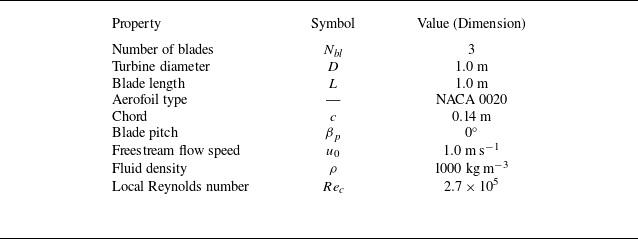


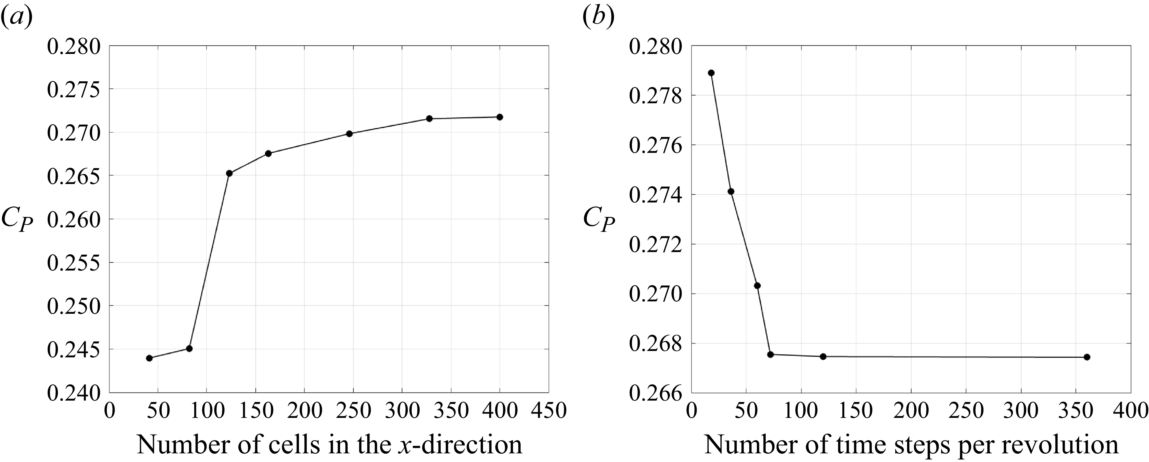
 72
 92.31%
 x
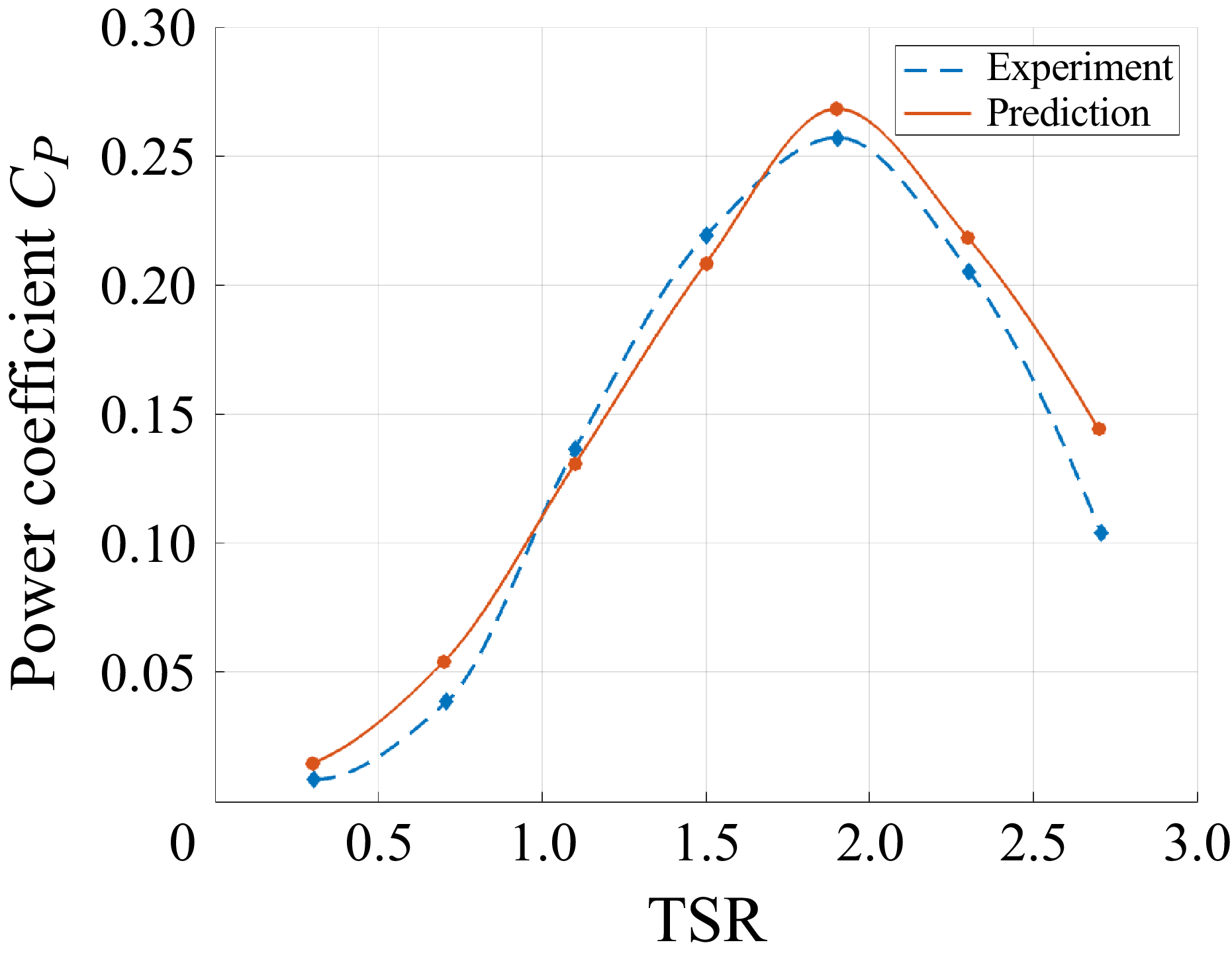
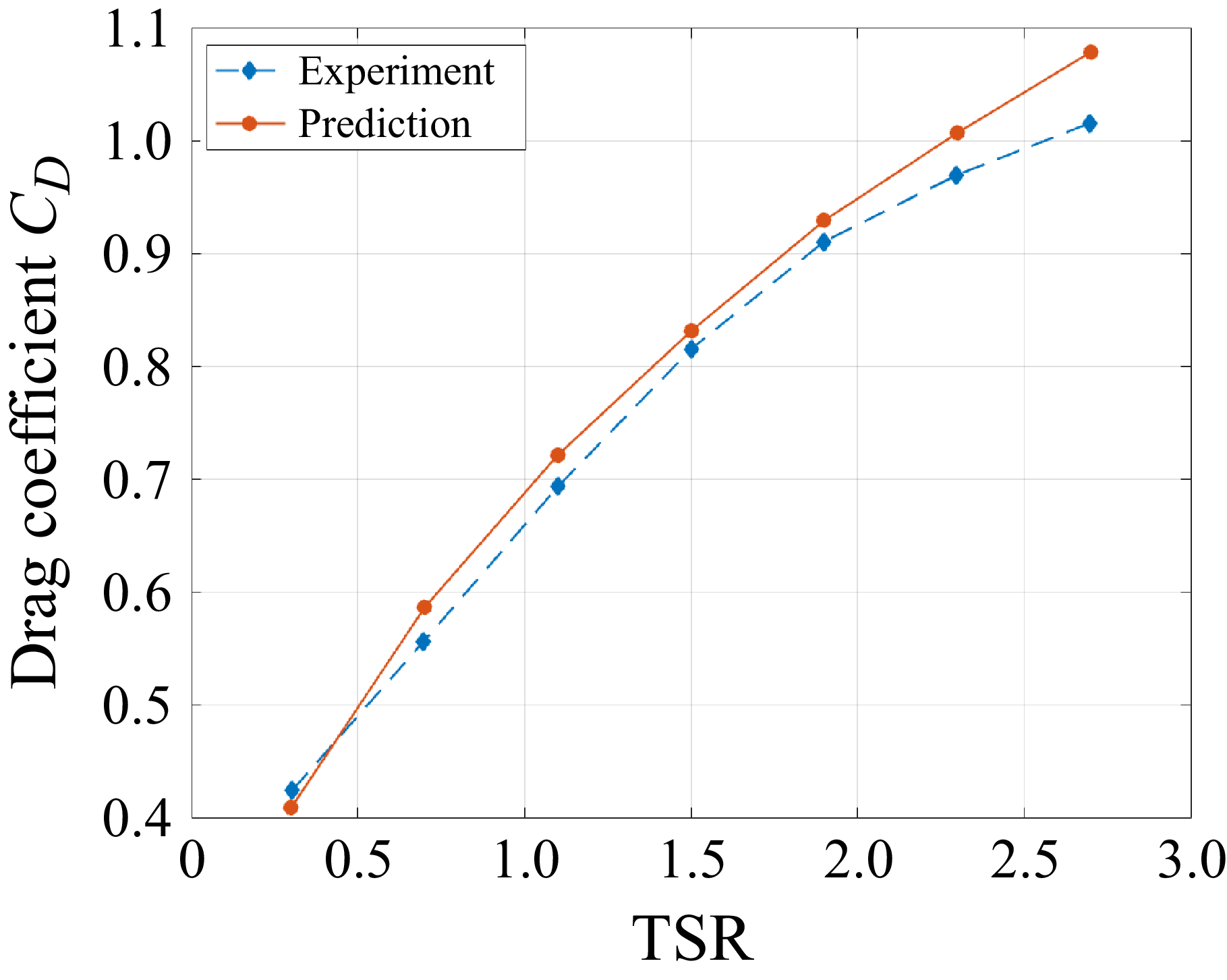

 z

 TSR=1.9
 x
 y
 z/H=0
 y
 z
 x/D=1

 TSR=1.9

 TSR=1.9


 TSR=1.9

 TSR=1.9

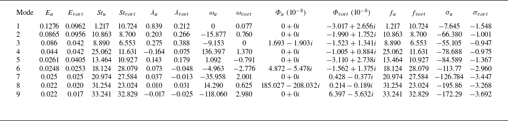
 TSR=1.9
 E
 St
 λ
 ω
 Φ
 σ
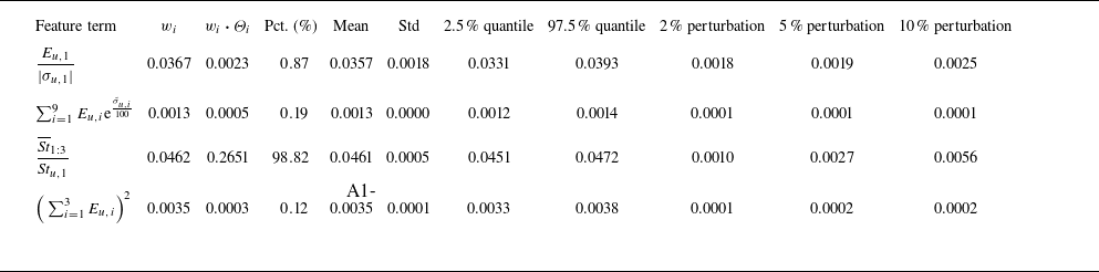
 CP
 TSR=1.9
 ±5%
 N=500


