1. Introduction
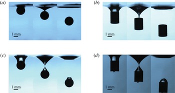
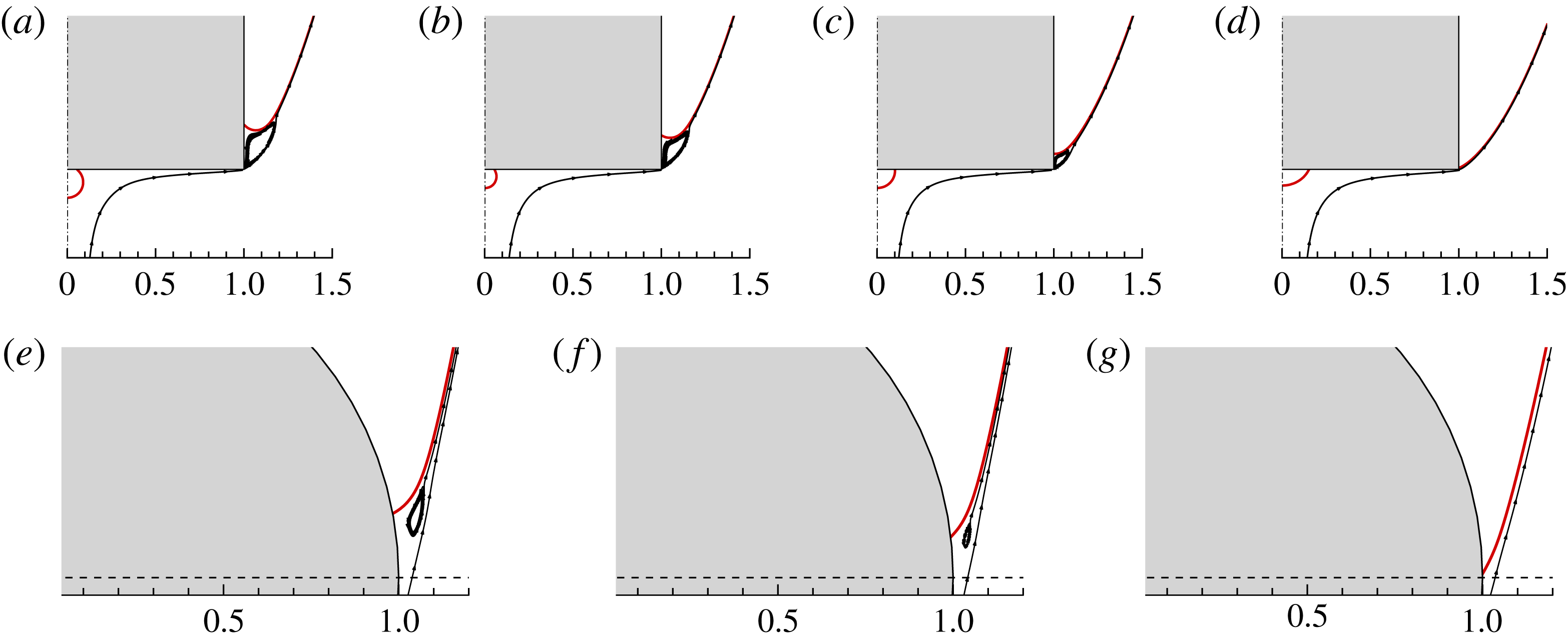
Typical scenarios of complete immersion (a,b) and bubble entrapment (c,d) during the impact of spheres (a,c) or cylinders (b,d) into a water pool. For complete immersion, hydrophilic objects are used (static contact angle
 ${\it\theta}\approx 30^{\circ }$
), and
 $U=0.28~\text{m}~\text{s}^{-1}$
(cylinder) and
 $0.30~\text{m}~\text{s}^{-1}$
(sphere). The snapshots are presented at a time interval of 5 ms. For the bubble entrapment, hydrophobic objects are used (
 ${\it\theta}\approx 110^{\circ }$
), and
 $U=0.48~\text{m}~\text{s}^{-1}$
(cylinder) and
 $0.71~\text{m}~\text{s}^{-1}$
(sphere). The snapshots are presented at a time interval of 5 ms (sphere) and 3 ms (cylinder).

Solid–liquid impact is ubiquitous in our everyday life, from dropping a sugar cube into coffee to diving into a pool. It is also utilized for locomotion of water-walking creatures, e.g. basilisk lizards produce air cavities by slapping their hind feet against the water, thereby obtaining the lift to keep them from sinking (Glasheen & McMahon Reference Glasheen and McMahon1996; Bush & Hu Reference Bush and Hu2006). The fluid flows in solid–liquid impact are characterized by air entrainment on the top of the objects (Grumstrup, Keller & Belmonte Reference Grumstrup, Keller and Belmonte2007; Gekle et al.
Reference Gekle, van der Bos, Bergmann, van der Meer and Lohse2008; Truscott & Techet Reference Truscott and Techet2009; Yan et al.
Reference Yan, Liu, Kominiarczuk and Yue2009), and may be simultaneously accompanied by complicated flow phenomena such as splash (Duez et al.
Reference Duez, Ybert, Clanet and Bocquet2007), pinch-off (Bergmann et al.
Reference Bergmann, van der Meer, Gekle, van der Bos and Lohse2009; Gekle et al.
Reference Gekle, Peters, Gordillo, van der Meer and Lohse2010) and liquid jets (Bergmann et al.
Reference Bergmann, van der Meer, Stijnman, Sandtke, Prosperetti and Lohse2006; Gekle et al.
Reference Gekle, Gordillo, van der Meer and Lohse2009; Gekle & Gordillo Reference Gekle and Gordillo2010). In the fascinating dynamic process of solid–liquid impact, the motion of the contact line (CL), where the phases of solid, liquid and gas meet, plays a crucial role. The CL is formed when the object comes into contact with the liquid, and at that moment it has a large speed relative to the object, due to the large difference in velocity between the impacting object and the surrounding liquid. The regimes of solid–liquid impact can be classified by the manner of CL motion on the object surface. For example, water entry of a small object is seen to follow three flow regimes, which are referred to here as complete immersion, bubble entrapment and cavity formation. In the regime of complete immersion, the CL converges at the peak of the object, and completely detaches from the object surface in the absence of air entrainment (see figure 1
a,b). In the regime of bubble entrapment, the CL moves upwards until the closure of the cavity. It eventually rests on the object surface, thereby entrapping a bubble on the top of the object (see figure 1
c,d). The regime of cavity formation is distinguished by pinning of the CL on the side of the object very shortly after the impact, and thereafter continuous elongation and expansion of the air cavity for a relatively long time (
 ${\sim}\!O(R_{0}/U)$
), where
 $R_{0}$
is the length scale of the impact object (the object radius in the present study) and
 $U$
is the impact velocity (see figure 3). Therefore, it is important to investigate the interaction between the local CL motion and the global flows, to improve our understanding of the complicated flow dynamics in solid–liquid impact.
Cavity formation and dynamics receive most attention of fluid dynamicists among the three flow regimes. The regime of cavity formation was experimentally found to be influenced by the combined effect of wettability, object geometry and the flow conditions. Duez et al. (Reference Duez, Ybert, Clanet and Bocquet2007) experimentally showed that an impact of a hydrophobic sphere more likely leads to a cavity accompanied by a loud splash, while a hydrophilic one does not produce any air entrainment. In the water entry of small spheres, a variety of cavity structures have been observed depending on the flow conditions (Aristoff & Bush Reference Aristoff and Bush2009), and the spheres were found to experience unsteady forces (Lee & Kim Reference Lee and Kim2008; Truscott, Epps & Techet Reference Truscott, Epps and Techet2012), which affect the shape of the air cavity (Aristoff et al. Reference Aristoff, Truscott, Techet and Bush2010). Impact objects with other geometries have also been considered, e.g. cylinders (Duclaux et al. Reference Duclaux, Caille, Duez, Ybert, Bocquet and Clanet2007; Gekle et al. Reference Gekle, van der Bos, Bergmann, van der Meer and Lohse2008) and disks (Bergmann et al. Reference Bergmann, van der Meer, Gekle, van der Bos and Lohse2009; Peters, van der Meer & Gordillo Reference Peters, van der Meer and Gordillo2013). More previous studies can be found in a recent review article (Truscott, Epps & Belden Reference Truscott, Epps and Belden2014).
Cavity dynamics in solid–liquid impact are also investigated theoretically and numerically. Duclaux et al. (Reference Duclaux, Caille, Duez, Ybert, Bocquet and Clanet2007) developed an analytical model related to Rayleigh–Besant problems for the time evolution of the cylindrical cavity. In this model, the CL is assumed to be pinned on the object surface, and, in particular, the position and the slope of the interface at the CL are needed for the analytical solution of the cavity shape. This model has been extensively used for the analysis of cavity dynamics under different circumstances (Aristoff & Bush Reference Aristoff and Bush2009; Bergmann et al. Reference Bergmann, van der Meer, Gekle, van der Bos and Lohse2009). Gaudet (Reference Gaudet1998) used a boundary element method to simulate the water entry of circular disks into a liquid pool, with the assumption of a pinned CL at the lower edge of the disk. It should be noted that the theoretical analysis and numerical simulation above are based on the assumptions of potential flows and a free surface. In contrast, Vella & Li (Reference Vella and Li2010) solved the Navier–Stokes equations to investigate the unsteady motion of a small cylinder after impact, with the assumption of a pinned CL at the cylinder surface. Do-Quang & Amberg (Reference Do-Quang and Amberg2009) introduced a moving CL model in numerical simulations of two-phase flows based on Navier–Stokes equations, thereby allowing for dynamic wetting on the object surface.
The CL dynamics was found to influence the flow phenomena in solid–liquid impact. Duez et al. (Reference Duez, Ybert, Clanet and Bocquet2007) proposed that the splash was caused by the detachment of the liquid film that wets the sphere surface, i.e. a wetting transition. A wetting transition occurs when the interface moves faster than the maximum CL speed allowed,
 ${\sim}\!{\it\sigma}/{\it\mu}$
, where
 ${\it\sigma}$
is the surface tension and
 ${\it\mu}$
is the viscosity. It accounts for the splash crown that occurs at the early stage of the impact. At the late stage of the impact, the CL was seen to be eventually pinned on the surface of the impact object in the cavity formation, more precisely, near the equator of spheres (Duez et al.
Reference Duez, Ybert, Clanet and Bocquet2007; Aristoff & Bush Reference Aristoff and Bush2009) or apparently at the edge of disks (Bergmann et al.
Reference Bergmann, van der Meer, Gekle, van der Bos and Lohse2009; Gekle et al.
Reference Gekle, Peters, Gordillo, van der Meer and Lohse2010). Clearly, this is very different from the regime of bubble entrapment, in which the cavity closure increases the capillary pressure and leads to CL pinning. Instead, it is reasonable to anticipate that the local flow in the vicinity of the CL plays an important role in the process of CL pinning in the cavity formation. However, it remains unclear why and where the initially moving CL is pinned on the object surface, and how the geometry of the impact object affects the CL pinning.
In this paper we investigate the CL pinning in the cavity formation with impact objects of different geometries by means of simulations and experiments. We consider here inertia-dominated solid–liquid impact, with the Weber number
 $We$
(
 $={\it\rho}U^{2}R_{0}/{\it\sigma}$
) of the order of
 $10$
to
 $10^{2}$
and the Reynolds number
 $Re$
(
 $={\it\rho}UR_{0}/{\it\mu}$
) of the order of
 $10^{3}$
, where
 ${\it\rho}$
is the liquid density. The effect of gravitational force is negligible here since the Froude number
 $Fr=U^{2}/(gR_{0})\sim O(10^{4})$
, where
 $g$
is the gravitational acceleration. Experimental results are used to validate the numerical simulation, and the latter provides detailed flow structures and cavity shapes, which are analysed and compared against the theoretical analyses. The numerical method combines an axisymmetric Navier–Stokes solver with a diffuse-interface model for interface tracking (Ding, Spelt & Shu Reference Ding, Spelt and Shu2007) and a moving CL model (Ding & Spelt Reference Ding and Spelt2007; Liu & Ding Reference Liu and Ding2015), thereby allowing for simulation of the impact process with dynamic wetting. We also study the subsequent radial expansion of the air cavity and the vertical propagation of the ripples arising from the impact, to seek the link between the local pinned meniscus and the global cavity dynamics. In the experiments and simulations, we mainly consider two types of impact object, i.e. spheres and circular cylinders; however, other geometries such as disks and spheroids are also considered in the numerical simulation when studying the critical conditions for the onset of cavity formation in terms of the dimensionless impact velocity.
The paper is organized as follows. The methodologies in the experiments and simulations are introduced in § 2. The overall flow behaviour of cavity formation and the validation of the numerical schemes are shown in § 3.1. In § 3.2, the flow structures and the position of the pinned CL are shown, and the effects of wettability, inertia, surface tension and object geometry on the pinned CL are analysed based on a force balance on the interface near the CL. The radial expansion of the air cavity and the vertical propagation of the ripples are compared against theoretical predictions in §§ 3.3 and 3.4 respectively. Finally, the critical conditions for the onset of cavity formation are investigated in § 3.5 for a variety of geometries, and the geometrical effects are shown to be related to the flow separation.
2. Methodology
2.1. Numerical methods
2.1.1. Diffuse-interface model and governing equations
In order to gain further insight into the flow behaviour, numerical simulations are performed by solving the axisymmetric Navier–Stokes equations in the (
 $r,z$
) plane. The interface is represented by the volume fraction of the liquid,
 $C$
, and its time evolution is governed by the convective Cahn–Hilliard equation (Jacqmin Reference Jacqmin1999),
 $$\begin{eqnarray}\frac{\partial C}{\partial t}+\boldsymbol{{\rm\nabla}}\boldsymbol{\cdot }(\boldsymbol{u}C)=\frac{1}{Pe}{\rm\nabla}^{2}{\it\Psi},\end{eqnarray}$$
where
 $\boldsymbol{u}$
is the flow velocity,
 ${\it\Psi}(={\it\xi}^{\prime }(C)-Cn^{2}{\rm\nabla}^{2}C)$
is the chemical potential and
 ${\it\xi}=C^{2}(1-C)^{2}/4$
is the bulk energy density. The Cahn number
 $Cn$
represents a dimensionless measure of the thickness of the diffuse interface, and the Péclet number
 $Pe$
(
 $=UL/(M{\it\Psi}_{c})$
) represents the relative significance of convective fluxes to the diffusive fluxes, where
 $M$
is the mobility and
 ${\it\Psi}_{c}\sim O(1)$
is the characteristic value of the chemical potential. To achieve the sharp-interface limit with continuous mesh refinement,
 $Pe\sim Cn^{-1}$
is recommended by Magaletti et al. (Reference Magaletti, Picano, Chinappi, Marino and Casciola2013), and we use
 $Pe=1/Cn$
in the present study.
The density and viscosity ratios of the gas to the liquid are
 ${\it\lambda}_{{\it\rho}}$
and
 ${\it\lambda}_{{\it\mu}}$
, and their values are set to
 $0.001$
and
 $0.025$
respectively. Since the gravitational effect is negligibly small compared with the impact inertia (
 $Fr\sim O(10^{4})$
), the gravitational force is neglected in the simulations. The motion of fluids is governed by the dimensionless Navier–Stokes equations and continuity equation,
 $$\begin{eqnarray}\displaystyle & \displaystyle {\it\rho}\left(\frac{\partial \boldsymbol{u}}{\partial t}+\boldsymbol{u}\boldsymbol{\cdot }\boldsymbol{{\rm\nabla}}\boldsymbol{u}\right)=-\boldsymbol{{\rm\nabla}}p+\frac{1}{Re}\boldsymbol{{\rm\nabla}}\boldsymbol{\cdot }[{\it\mu}(\boldsymbol{{\rm\nabla}}\boldsymbol{u}+\boldsymbol{{\rm\nabla}}\boldsymbol{u}^{\text{T}})]+\frac{\boldsymbol{f}_{s}}{We}, & \displaystyle\end{eqnarray}$$
 $$\begin{eqnarray}\displaystyle & \displaystyle \boldsymbol{{\rm\nabla}}\boldsymbol{\cdot }\boldsymbol{u}=0, & \displaystyle\end{eqnarray}$$
 $\boldsymbol{f}_{s}=6\sqrt{2}{\it\Psi}\boldsymbol{{\rm\nabla}}C/Cn$
denotes the surface tension force (Ding et al.
Reference Ding, Spelt and Shu2007). The dimensionless averaged density
 ${\it\rho}$
and viscosity
 ${\it\mu}$
are defined as
 $$\begin{eqnarray}\displaystyle & {\it\rho}=C+{\it\lambda}_{{\it\rho}}(1-C), & \displaystyle\end{eqnarray}$$
 $$\begin{eqnarray}\displaystyle & {\it\mu}=C+{\it\lambda}_{{\it\mu}}(1-C). & \displaystyle\end{eqnarray}$$
The method is capable of simulating two-phase flows with large density and viscosity ratios (Ding et al.
Reference Ding, Spelt and Shu2007). Wetting conditions are applied at the CLs to serve as the boundary conditions for
 $C$
at the solid walls, and we use the geometric wetting conditions for flat substrates (Ding & Spelt Reference Ding and Spelt2007) and the characteristic wetting condition for curved substrates (Liu & Ding Reference Liu and Ding2015). We assume that the speed of the object does not change in the short duration of the impact (it is confirmed by experiments that the change in object speed is insignificant). For convenience, we solve the equations expressed in a reference frame having its origin fixed with the object, and let the liquid move upwards at a constant speed of
 $U$
at the lower boundary. Unless otherwise stated, we refer to this reference frame throughout the text.
The wettability of the impact object is prescribed by a contact angle of fixed value
 ${\it\theta}_{s}$
. Here,
 $R_{0}$
,
 $U$
and
 $T$
(
 $=R_{0}/U$
) are chosen as the characteristic length, velocity and time respectively. All of the simulations are conducted in a domain of
 $8\times 16$
, and the centre of the objects is located at (0, 6). A uniform Cartesian grid is used for spatial discretization, and
 $Cn=0.5{\rm\Delta}x$
, where
 ${\rm\Delta}x$
is the mesh size. If we define the interface region by
 $0.05\leqslant C\leqslant 0.95$
, which contains 98.5 % of the surface tension force (Jacqmin Reference Jacqmin1999), the interface thickness is approximately
 $8.26Cn$
(or
 $4.13{\rm\Delta}x$
in the present study), which is sufficient to resolve the interface.
In the simulations we used the same
 $We$
and
 $Re$
as in the experiments, but a slightly larger contact angle. Our previous numerical study of fast spreading of a droplet on a substrate (Ding et al.
Reference Ding, Li, Zhang, Sui, Spelt and Thoroddsen2012) showed that, when setting
 ${\it\theta}_{s}$
to the static contact angle
 ${\it\theta}$
in the experiment, we need a very small
 $Cn$
(
 ${\sim}O(10^{-4})$
) to achieve quantitative agreement with the experimental results. Unfortunately, very small
 $Cn$
also suggests very expensive computation. At an affordable computational cost (
 $Cn\sim O(10^{-3})$
), choosing a
 ${\it\theta}_{s}$
slightly larger than
 ${\it\theta}$
can also capture the dynamics of the interface and CL in droplet spreading (Ding et al.
Reference Ding, Li, Zhang, Sui, Spelt and Thoroddsen2012). Alternatively, one can use the macroscopic (or dynamic) contact-angle models (Carlson, Do-Quang & Amberg Reference Carlson, Do-Quang and Amberg2009; Yue & Feng Reference Yue and Feng2011; Sui & Spelt Reference Sui and Spelt2013), in which the contact angle is a function of the microscopic contact angle and the CL speed.
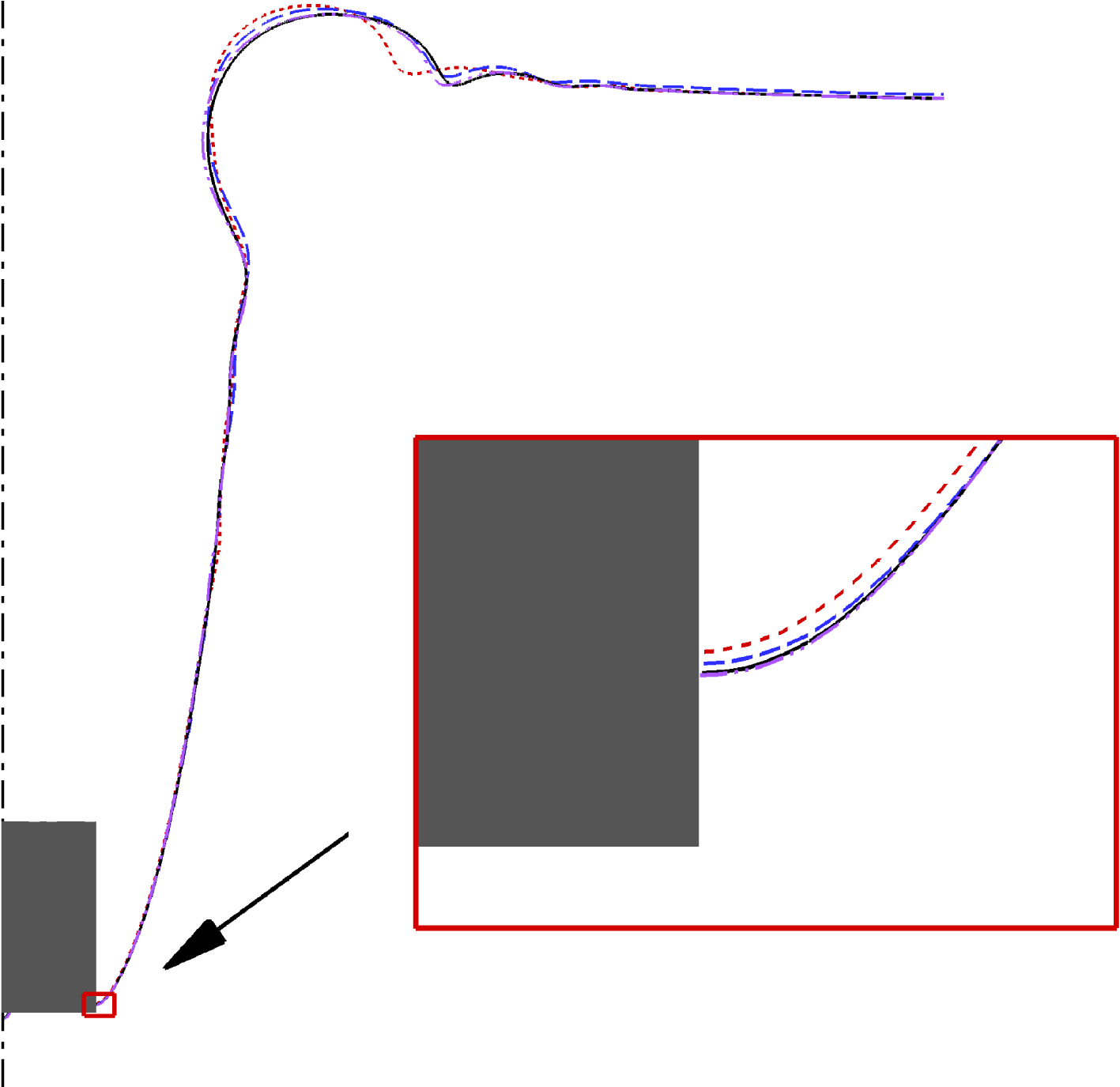
Snapshots of the impact of a circular cylinder at the time
 $t=9.4$
with
 $We=40$
,
 $Re=1680$
and
 ${\it\theta}_{s}=90^{\circ }$
. The different curves represent the numerical results obtained on the meshes of different resolution, and
 ${\rm\Delta}x=0.015$
(dashed),
 $0.012$
(long dashed),
 $0.01$
(solid) and
 $0.008$
(dash-dot-dotted). The inset shows the zoomed-in view of the interface in the vicinity of the pinned CL.

2.1.2. Convergence study
It is important in numerical experiments to ensure that a sufficiently fine mesh is used so that the flow structures occurring in the dynamic process are well resolved. We have conducted numerical experiments for the impact of a circular cylinder at
 $We=40$
,
 $Re=1680$
and
 ${\it\theta}_{s}=90^{\circ }$
, to check the convergence of the position of the pinned CL on different meshes. Figure 2 shows snapshots of the cavity shape with
 ${\rm\Delta}x=0.015$
,
 $0.012$
,
 $0.01$
and
 $0.008$
. It is clear that the results converge with the mesh refinement, in terms of the interface shape and the position of the pinned CL. In particular, the results with
 ${\rm\Delta}x=0.01$
are virtually overlapped with those on the finest mesh, i.e.
 ${\rm\Delta}x=0.008$
, on which the pinned CL has a distance of
 $0.07$
from the lower edge of the cylinder. We have also checked that the CL pinning is not sensitive to the discretization of the corner of the cylinders and disks in the present study. Therefore, a Cartesian mesh of
 $0.01$
mesh size and a fixed
 $Cn$
of
 $0.005$
are used in all of the simulations.
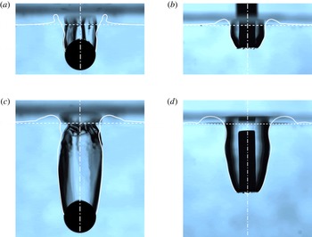
Typical scenarios of formation and growth of an air cavity in solid–water impact. (a,c) Water entry of a sphere with
 $R_{0}=1~\text{mm}$
,
 $U=3.35~\text{m}~\text{s}^{-1}$
and
 ${\it\theta}=100^{\circ }\pm 10^{\circ }$
(
 $We=156$
,
 $Re=3350$
and
 ${\it\theta}_{s}=130^{\circ }$
in the simulation). The reference frame has its origin fixed with respect to the laboratory, and the times starting from the impact are
 $t=2.9$
(a) and
 $6.7$
(c). (b,d) Water entry of a circular cylinder with
 $R_{0}=1~\text{mm}$
,
 $U=1.26~\text{m}~\text{s}^{-1}$
and
 ${\it\theta}=100^{\circ }\pm 10^{\circ }$
(
 $We=22.2$
,
 $Re=1264$
and
 ${\it\theta}_{s}=120^{\circ }$
in the simulation), at times
 $t=2.1$
(b) and
 $6.1$
(d). The numerical results (white solid lines) are superimposed on the experimental ones, and the white dashed lines show the water surface in the simulations.

2.2. Experimental set-up
Our experimental set-up includes polished steel objects (circular cylinders or spheres) of radius
 $R_{0}=1~\text{mm}$
. The steel object is initially held by an electromagnetic device and then released at a certain height (ranging from 1 mm to 620 mm) above a water container with dimensions of
 $73~\text{mm}\times 40~\text{mm}\times 60~\text{mm}$
. The container is illuminated by a 150 W fluorescent bulb, and a diffuser is used to provide uniform lighting. The free fall of the object produces an impact speed ranging from 0.14 to
 $3.48~\text{m}~\text{s}^{-1}$
, at which the regimes of complete immersion, bubble entrapment and cavity formation are observed. The dynamics of the subsequent cavity formation is recorded by a high-speed camera at 3600 frames s−1, which is also used to accurately compute the impact speed. The resolution is set to
 $768\times 768$
pixels with a field view of
 $1.66~\text{cm}\times 1.66~\text{cm}$
, and it thus yields a
 $214\,000~\text{px}~\text{cm}^{-2}$
magnification. Distilled water is used here, and has a surface tension coefficient of
 $0.0725~\text{N}~\text{m}^{-1}$
and a viscosity of
 $0.001~\text{Pa}~\text{s}$
. The impact objects are cleaned with distilled water and dried in air for two hours before use. The wettability of the object is measured by the static contact angle
 ${\it\theta}$
in the experiments, and the value of
 ${\it\theta}$
is observed to be in the range of
 $100^{\circ }\pm 10^{\circ }$
. The root mean square displacement of the roughness is of the order of
 $0.1~{\rm\mu}\text{m}$
.
3. Results and discussion
3.1. Cavity formation: overall interface dynamics
Snapshots of cavity formation during the water entry of a sphere and a cylinder are shown in figure 3, in which the numerical results are superimposed on the experimental ones. It is seen that the initially moving CLs stop on the side of the objects, more precisely, slightly above the sphere equator and near the bottom edge of the cylinder. The dynamics of the cavity formation is also shown in the supplementary movies available at http://dx.doi.org/10.1017/jfm.2015.574. In the simulation, the bubble entrapment is seen on the bottom of the cylinder, but this phenomenon is not observed in the sphere case. This is consistent with experimental observations. On the other hand, a few flow features in the experiments are not observed in the simulations. For example, ring bubbles are formed on the bottom of the cylinder, which coalesce into one bubble in the simulation but break up into tiny bubbles in the experiment. Moreover, in the sphere case capillary waves swirling around the cavity wall are seen in the experiment, but are absent in the simulation. The discrepancies between our experimental observations and numerical simulations are due to the assumption of axisymmetric flows in the simulations. Nevertheless, these three-dimensional flow features appear to have an insignificant effect on the CL pinning of the air cavity with respect to the position of the pinned CL and the interface shape in the vicinity of the CL. Clearly, an overall agreement is achieved between the numerical and experimental results. Therefore, in the following sections we investigate the CL pinning and the subsequent cavity formation with the aid of axisymmetric simulations.
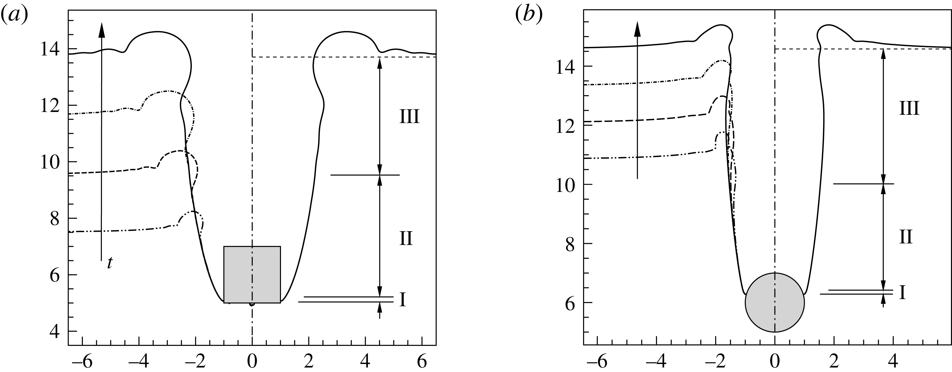
Cavity formation generated by the impact of a circular cylinder (a) and a sphere (b). The left half shows the snapshots of the cavity at various times, while the right half illustrates the interface regions. In (a),
 $We=40$
,
 $Re=1680$
and
 ${\it\theta}_{s}=90^{\circ }$
, and the snapshots start from
 $t=2.5$
after the impact, with a time interval of
 $2$
. In (b),
 $We=300$
,
 $Re=3000$
and
 ${\it\theta}_{s}=90^{\circ }$
, and the snapshots start from
 $t=6.4$
, with a time interval of
 $1.2$
. The arrows indicate increase of time.

Figure 4 shows the cavity dynamics after the CL is pinned at the surface of the objects with different geometries. It is seen in both impact cases that the lower part of the air cavity gradually evolves into a quasi-steady state such that the snapshots at different times are overlapped; thereafter, the air cavity keeps increasing in length and expanding in radius, with ripples propagating outwards on the horizontal water surface and downwards along the cavity surface at the same time. Three interface regions are identified during the formation and growth of the air cavity according to the local flow structures and interface features, i.e. pinned meniscus, radial expansion and ripple propagation (figure 4).
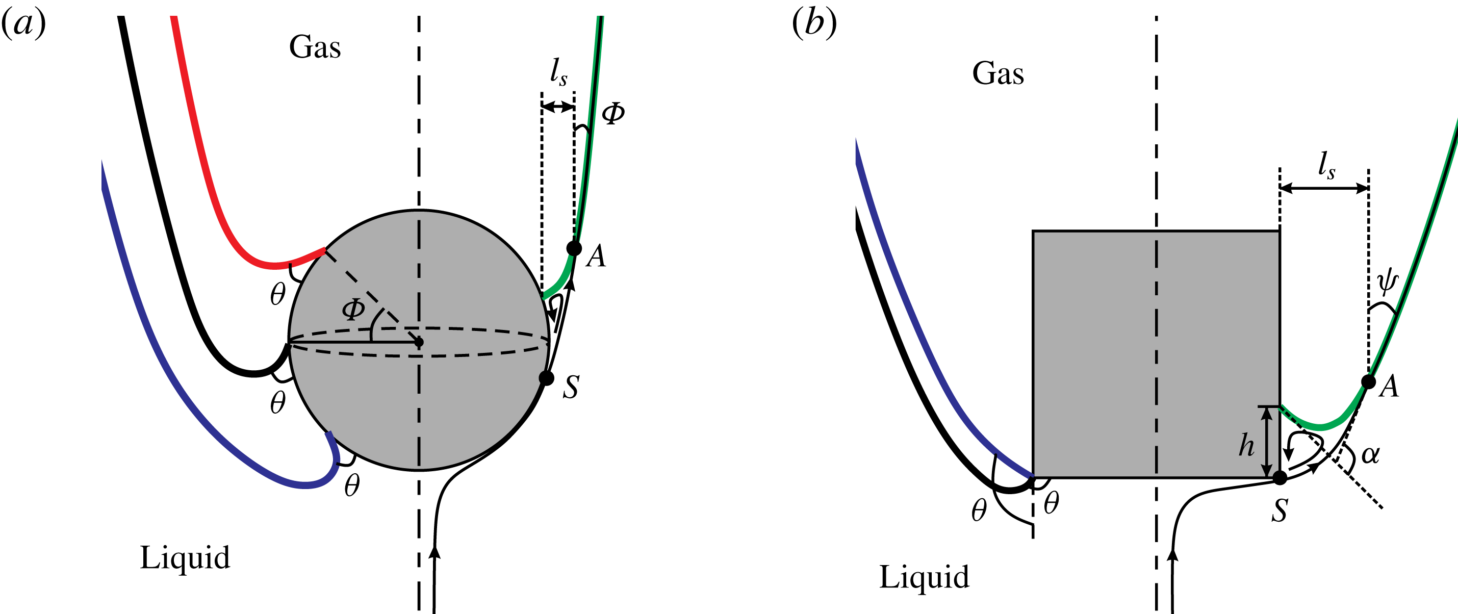
Pinned meniscus refers here to the bent interface near the bottom of the air cavity, particularly the part starting from the pinned CL to the point at which the streamline near the axis of symmetry (or surface streamline) merges with the interface (figure 5). Radial expansion corresponds to the smooth part of the air cavity above the pinned meniscus, and has lower curvature compared with the pinned meniscus. Ripple propagation refers to the wavy part of the air cavity near the free surface. The dynamics of the air cavity is characterized by the development of and competition among these three interface regions.
A sketch of the pinned meniscus and characteristic flow patterns for a sphere (a) and a circular cylinder (b). Some relevant parameters in the result analysis are also provided here. In the two subfigures, the possible stationary menisci are shown in the left half and the flow patterns are illustrated in the right half. In particular, the curve with arrows is the ‘surface streamline’ which starts near the axis of symmetry and merges with the interface (thick green line) at the point
 $A$
. The pinned meniscus is referred to as the interface between the CL and
 $A$
, and
 ${\it\alpha}$
is the measure of the bending of the pinned meniscus.

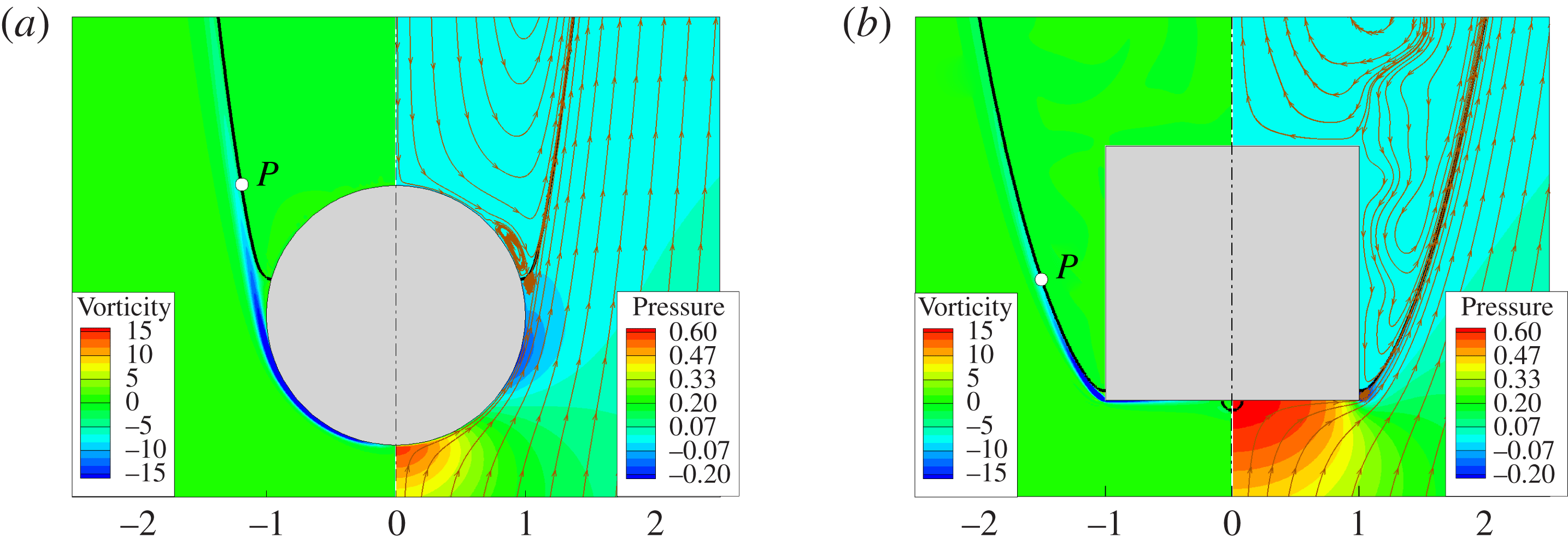
Flow structures in the vicinity of the menisci at
 ${\it\theta}_{s}=90^{\circ }$
: (a) sphere at
 $We=300$
and
 $Re=3000$
and (b) circular cylinder at
 $We=40$
and
 $Re=1680$
. The thick solid lines are the gas–liquid interfaces, and the curves with arrow heads are the streamlines, where the arrows indicate the flow direction. The contours represent the pressure
 $\bar{p}$
(
 $=p-p_{\infty }$
) and the scaled vorticity
 ${\it\lambda}_{{\it\mu}}\boldsymbol{{\rm\nabla}}\times \boldsymbol{u}$
, where
 $p_{\infty }$
is the ambient pressure far from the cavity.

3.2. Pinned meniscus
3.2.1. Flow structure and resting position
Typical flow structures around a pinned meniscus are shown in figure 6, in terms of streamlines, vorticity in the fluid and pressure. It is noticeable that the surface streamline leaves the object surface (at the separation point
 $S$
below the pinned CL as in figure 5), i.e. flow separation. We emphasize that flow separation was observed in all of the numerical simulations of cavity formation, suggesting that it is probably necessary for the occurrence of an air cavity. In the present case, the flow separation leads to a steady liquid eddy attached to the pinned CL. Recirculating flows are also seen in the gas; however, their effects on the cavity shape are negligible because of the rather low density and viscosity of the gas. Therefore, only contours of the scaled vorticity (defined as
 ${\it\lambda}_{{\it\mu}}\boldsymbol{{\rm\nabla}}\times \boldsymbol{u}$
) are shown in figure 6. The vorticity generated in the liquid is seen to be transported along the interface after detachment from the object surface, and then quickly diffuse into the surrounding fluids. Figure 6 shows that an adverse pressure gradient appears on the object surface, near the equator of the sphere and just above the lower edge of the cylinder. It is reasonable to anticipate that it would slow down the moving CL, and might pin the CL to the object surface if sufficiently strong.
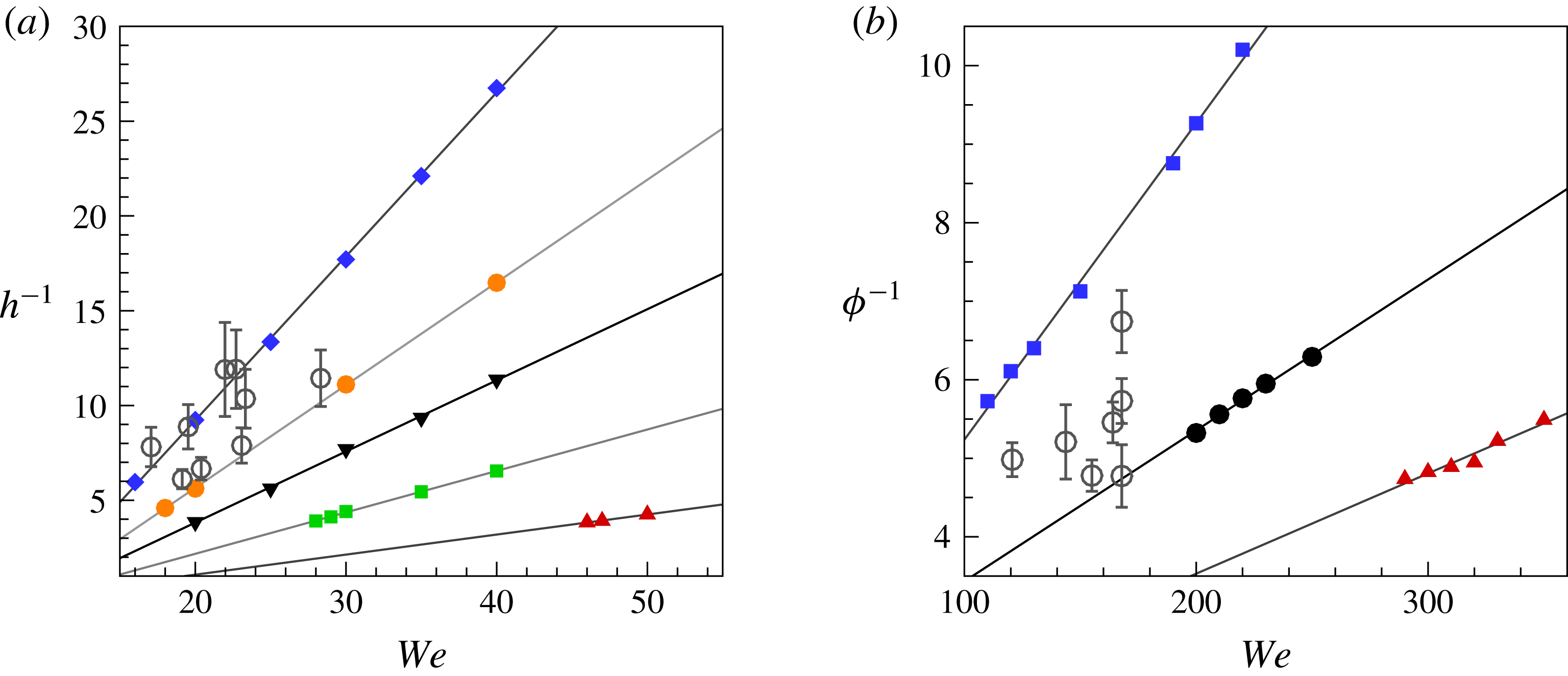
Position of the pinned CL on the object surface as a function of
 $We$
and
 ${\it\theta}_{s}$
for a cylinder (a) and a sphere (b). The filled symbols are the numerical results with various wettabilities and the empty circles with error bars are the experimental results (
 ${\it\theta}=100^{\circ }\pm 10^{\circ }$
). For the cylinder,
 ${\it\theta}_{s}=30^{\circ }$
(▴),
 $70^{\circ }$
(▪),
 $90^{\circ }$
(▾),
 $100^{\circ }$
(●),
 $110^{\circ }$
(
 $\blacklozenge$
); for the sphere,
 ${\it\theta}_{s}=90^{\circ }$
(▴),
 $110^{\circ }$
(●),
 $130^{\circ }$
(▪). It should be noted that the lowest
 $We$
is close to the critical
 $We$
for the onset of cavity formation. The straight lines are the linear fittings of the numerical results.

It was found in all of our experiments and simulations that the CL was pinned on the side of the cylinder and above the equator of the sphere. To quantitatively determine the position of the pinned CL relative to the object surface, we measure the distance
 $h$
from the pinned CL to the lower edge of the cylinder, and the latitude
 ${\it\phi}$
of the pinned CL on the sphere (figure 5). Figure 7 shows the position of the pinned CL as a function of
 $We$
and
 ${\it\theta}$
. It is interesting to see that
 $h$
and
 ${\it\phi}$
are inversely proportional to
 $We$
for the numerical results. Since the values of
 $h$
and
 ${\it\phi}$
are associated with the linear dimension of the steady eddy on the cylinder and sphere respectively, this suggests that the steady eddy shrinks with increase of impact inertia for both the sphere and the cylinder. This phenomenon is associated with the force balance at the pinned meniscus, which will be addressed in the following section. We notice that the values of
 $h$
and
 ${\it\phi}$
gradually approach zero with increase of
 $We$
, and similarly there are upper bounds for
 $h$
and
 ${\it\phi}$
with decrease of
 $We$
. In our simulations, approximately
 $h_{max}=0.3$
and
 ${\it\phi}_{max}=14^{\circ }$
. If the CL could not be pinned at these positions, the CL would continuously move towards the peak of the impact object, and the impact process would enter the regime of either bubble entrapment or complete immersion. The values of
 $h$
measured in experiments range from
 $0.086$
to
 $0.167$
with decrease of
 $We$
, and the experimental results are seen to lie between the numerical ones with
 ${\it\theta}_{s}=100^{\circ }$
and
 $110^{\circ }$
. The values of
 ${\it\phi}$
in experiments are in a narrow range, i.e. from
 $8^{\circ }$
to
 $12^{\circ }$
, with decrease of
 $We$
. It is seen that the experimental results are between the numerical results with
 ${\it\theta}_{s}=110^{\circ }$
and
 $130^{\circ }$
. The scattering of experimental data at similar Weber numbers is probably due to non-uniformity in the surface properties of the impact objects, such as wettability and roughness.
3.2.2. Force balance and geometric effects on interface bending
The interface in the vicinity of the CL is unavoidably bent because of the velocity difference between the moving CL and the interface. The occurrence of a pinned meniscus suggests the establishment of a balance between the resultant surface tension and the inertia at the pinned meniscus. The bending of the pinned meniscus,
 ${\it\alpha}$
, can be measured by the direction change of the tangential vectors at its two ends, i.e. the pinned CL and the point at which the surface streamline merges with the interface (i.e. point
 $A$
in figure 5). When the pinned meniscus stays on a smooth vertical substrate, e.g. as in the impact cases of circular cylinders (figure 5), we can geometrically obtain that
 $$\begin{eqnarray}{\it\alpha}={\rm\pi}-{\it\theta}-{\it\psi},\end{eqnarray}$$
where
 ${\it\psi}$
is the angle that the interface makes with the vertical at the point
 $A$
. Our simulations indicate that
 ${\it\psi}$
is mainly determined by the combined effects of inertia and surface tension, and weakly depends on the contact angle.
For a pinned meniscus resting on a smooth vertical substrate, the force balance in the vertical direction can be approximated by
 $$\begin{eqnarray}\int _{S_{I}}(p_{g}-p_{l})(\boldsymbol{n}_{I}\boldsymbol{\cdot }\boldsymbol{j})\,\text{d}S-{\it\sigma}\left(\oint _{CL}\cos {\it\theta}\,\text{d}l+\oint _{L_{A}}\cos {\it\psi}\,\text{d}l\right)=0,\end{eqnarray}$$
where the subscripts
 $l$
and
 $g$
indicate the pressure on the side of the liquid and gas phases respectively;
 $CL$
is the contact line and
 $L_{A}$
is the cross-section of the interface in the horizontal plane at the point
 $A$
;
 $\boldsymbol{n}_{I}$
is the unit vector normal to the interface and points away from the liquid;
 $\boldsymbol{j}$
is the vertical unit vector.
Given the negligible gas density,
 $p_{g}$
is roughly the ambient pressure. In the liquid, the velocity in the recirculating flows is rather low and
 $p_{l}$
is close to the pressure of the irrotational flows outside the standing eddies. Thus,
 $p_{l}$
can be estimated by Bernoulli’s equation such that
 $p_{l}\approx p_{g,\infty }+{\it\rho}(U^{2}-v_{max}^{2})$
, where
 $v_{max}$
(
 $={\it\gamma}U$
) is the maximum velocity around the blunt body,
 ${\it\gamma}>1$
is a geometry-dependent parameter and
 $p_{g,\infty }$
is the ambient pressure. With the knowledge of this and the size of the recirculating flow
 $l_{s}\ll R_{0}$
, we can further simplify (3.2), in a dimensionless form,
 $$\begin{eqnarray}\displaystyle We & {\sim} & \displaystyle (\cos {\it\theta}+\cos {\it\psi})R_{0}/l_{s}\nonumber\\ \displaystyle & {\sim} & \displaystyle 2\sin \left(\frac{{\it\alpha}}{2}\right)\sin \left({\it\theta}+\frac{{\it\alpha}}{2}\right)R_{0}/l_{s}.\end{eqnarray}$$
We note that the object geometry can significantly influence the value of
 ${\it\alpha}$
. Figure 5 shows some possible menisci that rest at different places on the sphere or circular cylinder. Clearly, the value of
 ${\it\alpha}$
depends on the position where the menisci stay. For example, the meniscus resting at the latitude of
 ${\it\phi}$
on the sphere has less bending than the meniscus at the equator by an amount of
 ${\it\phi}$
, if the tangential vector at point
 $A$
remains unchanged. This fact makes the upper hemisphere (i.e.
 ${\it\phi}\geqslant 0$
) more favourable for the CL to rest on than the lower one (i.e.
 ${\it\phi}<0$
), which is consistent with our experimental observations. For a circular cylinder, the distinguishable feature in geometry is the presence of sharp edges at its top and bottom. Even if the wetting properties on the two sides of the edge are the same, these sharp edges can cause an effective contact-angle hysteresis
 ${\rm\Delta}{\it\theta}$
, and
 ${\rm\Delta}{\it\theta}={\rm\pi}/2$
in the cylinder cases. Consequently, the value of
 ${\it\alpha}$
at the cylinder edges is allowed to be adjusted by an amount of
 ${\rm\Delta}{\it\theta}$
(figure 5). The effective contact-angle hysteresis tends to entrap the CL at the sharp edges (Sui, Ding & Spelt Reference Sui, Ding and Spelt2014). Taking the geometric effect into account, we obtain the following force balance for the sphere cases:
 $$\begin{eqnarray}\displaystyle We & {\sim} & \displaystyle (\cos ({\it\theta}+{\it\phi})+\cos {\it\psi})R_{0}/l_{s}\nonumber\\ \displaystyle & {\sim} & \displaystyle 2\sin \left(\frac{{\it\alpha}}{2}\right)\sin \left({\it\theta}+{\it\phi}+\frac{{\it\alpha}}{2}\right)R_{0}/l_{s}.\end{eqnarray}$$
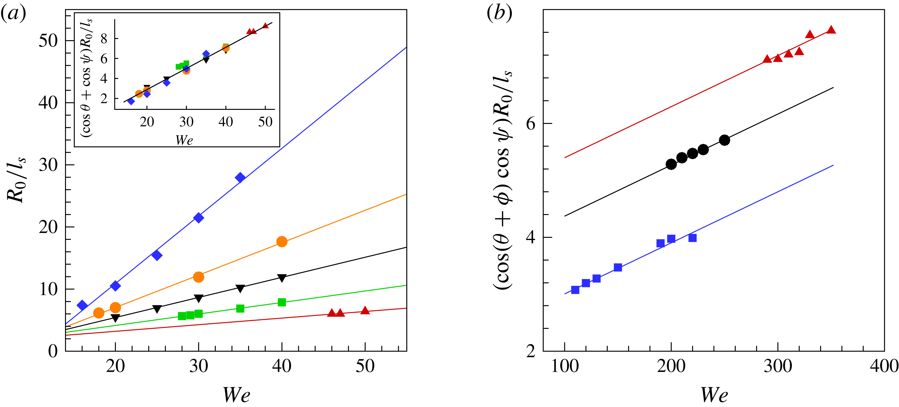
Variation of
 $l_{s}$
with
 $We$
for the impact of a cylinder (a) and a sphere (b). It should be noted that
 $Re\propto \sqrt{We}$
. The symbols are the numerical results with various wettabilities: for the cylinder,
 ${\it\theta}_{s}=30^{\circ }$
(▴),
 $70^{\circ }$
(▪),
 $90^{\circ }$
(▾),
 $100^{\circ }$
(●),
 $110^{\circ }$
(
 $\blacklozenge$
); for the sphere,
 ${\it\theta}_{s}=90^{\circ }$
(▴),
 $110^{\circ }$
(●),
 $130^{\circ }$
(▪). The lines are the corresponding linear data fittings. Inset:
 $(l_{s}/R_{0})^{-1}$
is rescaled by multiplying by
 $(\cos {\it\psi}+\cos {\it\theta})$
, and the data are apparently collapsed into a single line.

Equations (3.3) and (3.4) connect the interface bending (
 ${\it\alpha}$
), wettability (
 ${\it\theta}$
), eddy size (
 $l_{s}$
) and CL position (
 ${\it\phi}$
) with
 $We$
. Figure 8 quantitatively shows the variation of
 $l_{s}$
as a function of
 $We$
in our simulations, in which
 $l_{s}$
decreases with increase of
 $We$
, as expected from (3.3) and (3.4). In the case of cylinder impact,
 $l_{s}^{-1}$
appears to be linearly dependent on
 $We$
for a wide range of wettability, since the value of
 ${\it\psi}$
is not sensitive to
 $We$
for
 $10\leqslant We\leqslant 50$
. Furthermore, the results are apparently collapsed into a single line after being multiplied by
 $(\cos {\it\theta}+\cos {\it\psi})$
, where a typical value of
 ${\it\psi}$
(
 $=35^{\circ }$
) is used. For the case of sphere impact, because of the dependence of
 ${\it\phi}$
on
 $We$
, we cannot obtain
 $l_{s}^{-1}\propto We$
. Instead,
 $(\cos ({\it\theta}+{\it\phi})+\cos {\it\psi})l_{s}^{-1}$
is shown to be approximately proportional to
 $We$
, in agreement with the prediction from (3.4). The fitted lines appear to align, but do not collapse into a single line as in the case of cylinder impact. We suspect that this may be related to the occurrence of forced flow separation in the latter. It should be noted that although generally
 $We\gg 1$
in sphere impact, it is clear that the effect of surface tension cannot be neglected; in fact it is important for the local anchoring of the CL, thereby affecting the global cavity formation.
Size variation of standing eddies with the contact angle. (a–d) Impact of a cylinder into water at
 $We=40$
and
 $Re=1116$
;
 ${\it\theta}_{s}=45^{\circ }$
(a),
 $60^{\circ }$
(b),
 $90^{\circ }$
(c) and
 $120^{\circ }$
(d). (e–g) Impact of a sphere into water at
 $We=200$
and
 $Re=3800$
;
 ${\it\theta}_{s}=110^{\circ }$
(e),
 $130^{\circ }$
(f) and
 $150^{\circ }$
(g). The dashed line represents the equator of the sphere.

Assuming that
 $l_{s}$
,
 ${\it\phi}$
and
 ${\it\psi}$
are constants at the onset of cavity formation (indeed they do not change significantly in the numerical experiments), we can use (3.3) and (3.4) to predict the critical Weber number for cavity formation,
 $We_{cr}$
. It is clear that a hydrophilic object would requires a much higher
 $We_{cr}$
for the onset of cavity formation than a hydrophobic one, due to the sign change in the value of
 $\cos {\it\theta}$
. This is consistent with previous experimental observations by Duez et al. (Reference Duez, Ybert, Clanet and Bocquet2007).
Figure 9 illustrates the size variation of standing eddies in the impact of a cylinder (at
 $We=40$
and
 $Re=1116$
) and a sphere (at
 $We=200$
and
 $Re=3800$
), for a variety of contact angles. When the cylinder surface becomes more hydrophobic, it is clear that the interface bending becomes less significant, and the position of the pinned CL gradually shifts to the lower edge of the cylinder. Similarly, the position of the pinned CL in the sphere impact would shift to the equator of the sphere with increase of
 ${\it\theta}_{s}$
. This can be interpreted by (3.3) as follows:
 ${\it\alpha}$
decreases with increase of
 ${\it\theta}$
, thereby
 ${\it\alpha}\rightarrow 0$
and
 ${\it\theta}+{\it\alpha}/2\rightarrow {\rm\pi}$
; (3.3) suggests that as a result
 $l_{s}\rightarrow 0$
for a constant
 $We$
, i.e. the size of the standing eddy shrinks or even vanishes. That is,
 $l_{s}$
is related to the final size of the eddy, in agreement with the numerical results.
3.3. Radial expansion
Local anchoring of the CL on the side of the object makes a big difference in the global flow, and indicates the moment that an air cavity comes into existence. The air cavity proceeds to grow in length (at the rate of the impact velocity) and to expand in radius at the same time, influenced by a combined effect of inertia and surface tension. In previous investigations of cavity dynamics (Duclaux et al.
Reference Duclaux, Caille, Duez, Ybert, Bocquet and Clanet2007; Aristoff & Bush Reference Aristoff and Bush2009; Bergmann et al.
Reference Bergmann, van der Meer, Gekle, van der Bos and Lohse2009), it was suggested that at relatively high
 $We$
the cavity expansion follows the Rayleigh–Besant equation, with a velocity potential
 ${\it\Phi}$
of the form
 $$\begin{eqnarray}{\it\Phi}=\left\{\begin{array}{@{}ll@{}}RR_{t}\ln (r/R_{\infty }),\quad & R<r<R_{\infty },\\ 0,\quad & r>R_{\infty },\end{array}\right.\end{eqnarray}$$
where
 $R(t,z)$
is the radius of the cavity,
 $r$
is the radial coordinate and
 $R_{\infty }$
denotes the size of the region that the motion in the liquid extends over; the subscript
 $t$
represents differentiation with respect to time. It was previously assumed that
 $\ln (r/R_{\infty })\approx 1$
(Duclaux et al.
Reference Duclaux, Caille, Duez, Ybert, Bocquet and Clanet2007; Aristoff & Bush Reference Aristoff and Bush2009), which is also adopted in the present analysis.
Assuming that the flow is inviscid and taking the surface tension into account, the dynamics of the cavity wall is governed by a dimensionless unsteady Bernoulli equation,
 $$\begin{eqnarray}\frac{\partial {\it\Phi}}{\partial t}+\frac{R_{t}^{2}}{2}=\frac{{\it\kappa}}{We},\end{eqnarray}$$
where
 ${\it\kappa}$
is the local curvature of the cavity, and the characteristic length and velocity are
 $R_{0}$
and the impact velocity respectively.
Substitution of (3.5) into the unsteady Bernoulli equation (3.6) results in a variant of the Rayleigh–Besant equation for the evolution of
 $R$
with some manipulations (Duclaux et al.
Reference Duclaux, Caille, Duez, Ybert, Bocquet and Clanet2007; Aristoff & Bush Reference Aristoff and Bush2009),
 $$\begin{eqnarray}RR_{tt}+\frac{3}{2}{R_{t}}^{2}=\frac{1}{We}\left(\frac{R_{zz}}{(1+R_{z}^{2})^{3/2}}-\frac{1}{R(1+R_{z}^{2})^{1/2}}\right),\end{eqnarray}$$
where the subscript
 $z$
represents the corresponding differentiation with respect to
 $z$
.
Figure 4 showed that the air cavity entered a quasi-steady state in the frame of reference of the moving object after the CL was pinned, particularly for the interface region of radial expansion. In the following analysis, we also consider the Rayleigh–Besant equation (3.7) in the frame of reference of the moving object, and assume that
 $\text{d}z/\text{d}t=1$
for the whole cavity. Therefore, we can obtain
 $R_{z}=\text{d}R/\text{d}z=(\text{d}R/\text{d}t)/(\text{d}z/\text{d}t)=R_{t}$
, and similarly
 $R_{tt}=R_{zz}=(\text{d}R_{z}/\text{d}R)R_{z}$
. By substituting these into (3.7) and replacing all of the time derivatives, (3.7) can be rewritten as a steady ordinary differential equation,
 $$\begin{eqnarray}\frac{\text{d}R_{z}}{\text{d}R}=\left(R^{-1}(1+R_{z}^{2})^{-1/2}+\frac{3}{2}We\,R_{z}^{2}\right)(R_{z}(1+R_{z}^{2})^{-3/2}-We\,RR_{z})^{-1}.\end{eqnarray}$$
Equation (3.8) can be numerically solved by using a fourth-order Runge–Kutta method (see appendix A for details). However, the numerical solution of (3.8) requires the geometric information (
 $R$
and
 $R_{z}$
) on the cavity shape near the object to start the integration. The location of the starting point can have an effect on the accuracy of the numerical solution. It is seen in figure 6 that the vorticity that leaves the object surface is transported along the interface and eventually diffuses into the surrounding fluids. Because of the potential-flow assumption in our analysis, (3.8) is in principle not valid for the pinned meniscus, but for the interface region where the vorticity is negligibly small. Taking this into consideration, we do not choose the pinned CL as the starting point (as, e.g., in Aristoff & Bush Reference Aristoff and Bush2009), but the point above which the vorticity is rather weak (e.g.
 $P$
in figure 6). Accordingly, numerical results for
 $R$
and
 $R_{z}$
at the point
 $P$
are used as the initial conditions.
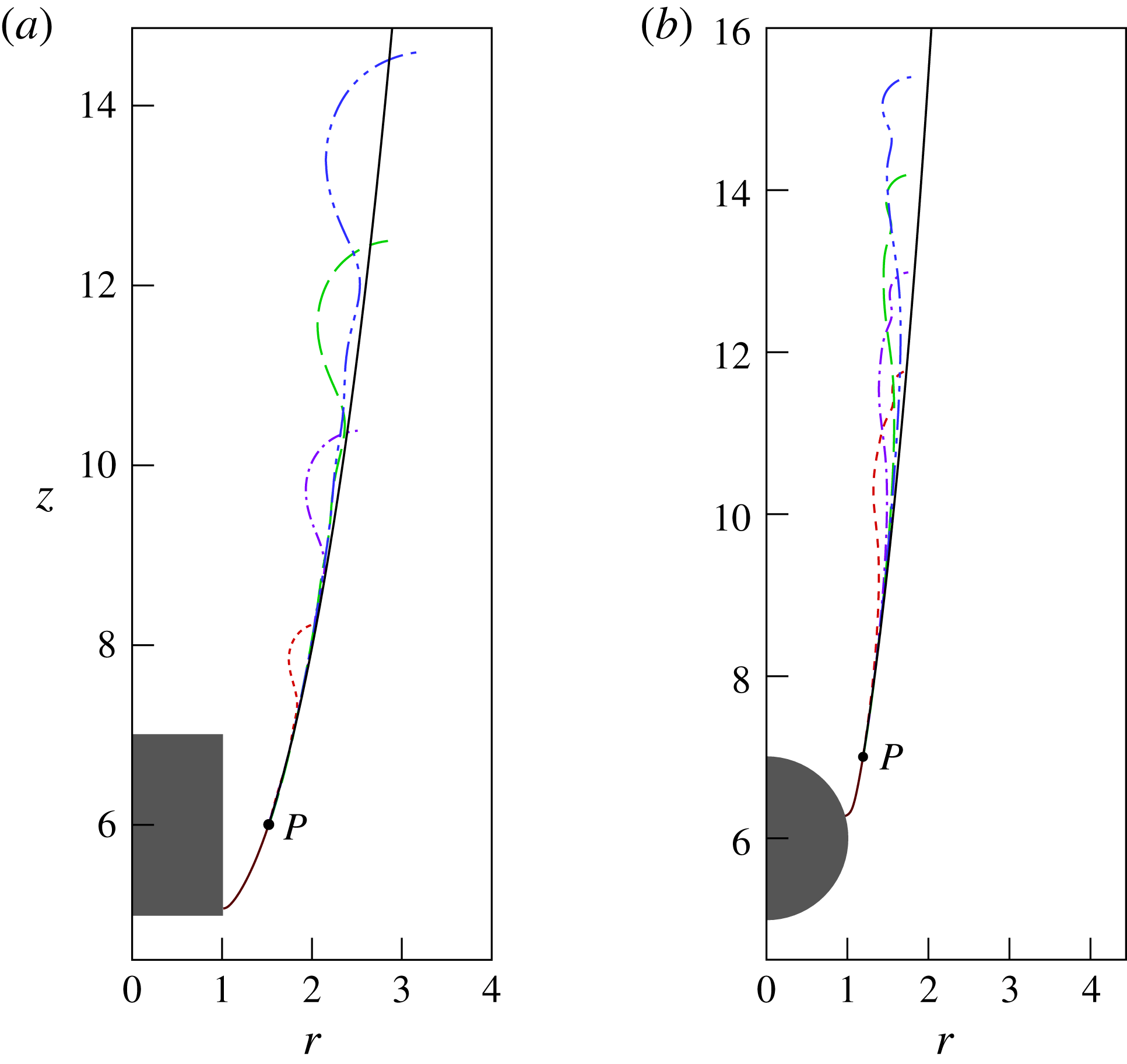
Comparison of cavity shapes between the theoretical prediction (solid curves) and the numerical results at different times: (a)
 $We=40$
,
 $Re=1680$
and
 ${\it\theta}_{s}=90^{\circ }$
, and
 $t=2.5$
(dashed),
 $4.5$
(dash-dotted),
 $6.5$
(long dashed) and
 $8.5$
(dashed-dot-dotted); (b)
 $We=300$
,
 $Re=3000$
and
 ${\it\theta}_{s}=90^{\circ }$
, and
 $t=6.4$
(dashed),
 $7.6$
(dash-dotted),
 $8.8$
(long dashed) and
 $10$
(dashed-dot-dotted). It should be noted that the upper end of the curve of the numerical results is the peak of the interface at the corresponding time.

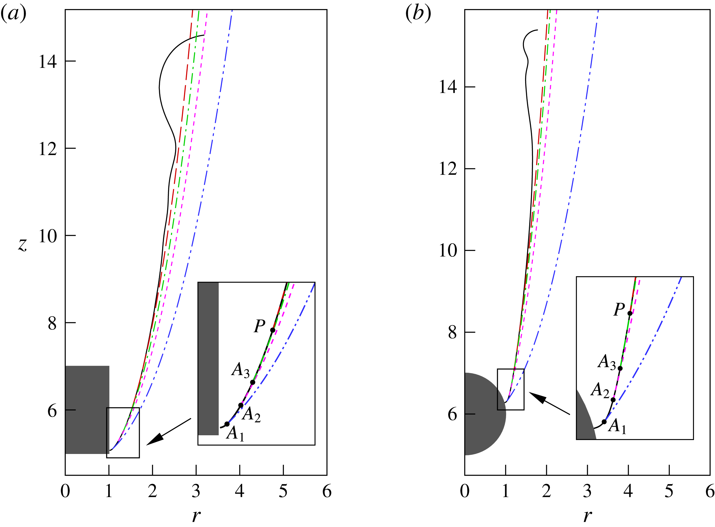
Comparison of cavity shapes between the theoretical predictions at different starting points. The solid curve denotes the numerical result for
 ${\it\theta}_{s}=90^{\circ }$
at a relatively long time after impact:
 $t=8.5$
for the cylinder impact at
 $We=40$
and
 $Re=1680$
, and
 $t=10$
for the sphere impact at
 $We=300$
and
 $Re=3000$
. The dash-dot-dotted, dashed, dash-dotted and long-dashed curves denote the theoretical predictions by (3.8) with
 $A_{1}$
,
 $A_{2}$
,
 $A_{3}$
and
 $P$
as the starting point. The inset shows the locations of these starting points.

For the two cases shown in figure 6, we seek the appropriate choice of
 $P$
by evaluating the scaled vorticity (
 ${\it\lambda}_{{\it\mu}}\boldsymbol{{\rm\nabla}}\times \boldsymbol{u}$
) along the interface from the CL. By setting the targeted value of the scaled vorticity to
 $5$
(which is roughly one order of magnitude less than the peak value of the scaled vorticity), we get the point
 $P$
at (
 $1.52,6.00$
) and accordingly
 $(R_{z})_{P}=0.315$
in the cylinder impact, and
 $P$
at (
 $1.19,7.00$
) and accordingly
 $(R_{z})_{P}=0.158$
in the sphere impact. Figure 10 shows a comparison of cavity shapes between the theoretical prediction and the numerical results at different times. The cavity shapes in the simulations appear to develop with time along the theoretical prediction, and, in particular, the part of the cavity wall with unnoticeable capillary waves is overlapped with the theoretical one. Clearly, the numerical result of (3.8) gives a good prediction of the cavity expansion for the impact of the cylinder and the sphere. To assess the sensitivity of the solution of (3.8) to the choice of
 $P$
, we compare the results starting at different locations (
 $A_{1}$
,
 $A_{2}$
,
 $A_{3}$
and
 $P$
) at/near the pinned meniscus in figure 11, in which
 $A_{1}$
,
 $A_{2}$
and
 $A_{3}$
are located at (
 $1.08,5.11$
), (
 $1.21,5.29$
) and (
 $1.33,5.51$
) in the case of cylinder impact, and (
 $1.03,6.32$
), (
 $1.09,6.46$
) and (
 $1.13,6.66$
) in the case of sphere impact. The values of
 $R_{z}$
were also obtained from the diffuse-interface simulation at these points. It is clear that the numerical integration of (3.8) is rather sensitive to the choice of the starting point. In particular, the result of using
 $A_{1}$
, i.e. the closest point to the pinned meniscus, significantly deviates from the diffuse-interface simulation.
We also note that the effect of object geometry is not taken into account by the theoretical model (3.8), and thus it must be reflected through the values of
 $R$
and
 $R_{z}$
at
 $P$
, which are determined by the shape of the pinned meniscus. In this sense, the interfacial information at
 $P$
connects the local CL flows with the global cavity dynamics. The numerical results in figure 10 indicate that the pinned meniscus region remains unchanged with time; in contrast, both the regions of radial expansion and ripple propagation expand with time. The growth rate of the latter two interface regions depends on the travelling of the capillary waves, which is analysed in § 3.4.
3.4. Ripple propagation
We consider here the vertical propagation of the capillary waves along the cavity wall. The ripples arising from the impact not only spread on the horizontal plane (figure 4), but also propagate vertically, simultaneous with the elongation and expansion of the air cavity (figure 10). To measure the capillary waves on the air cavity, we use the inertial frame of reference in this section. The variation of the cavity wall in the absence radial expansion is represented by
 ${\it\delta}R=R_{th}-R_{num}$
, where
 $R_{th}$
is the theoretical prediction of the cavity wall for radial expansion, i.e. the solution of (3.8), and
 $R_{num}$
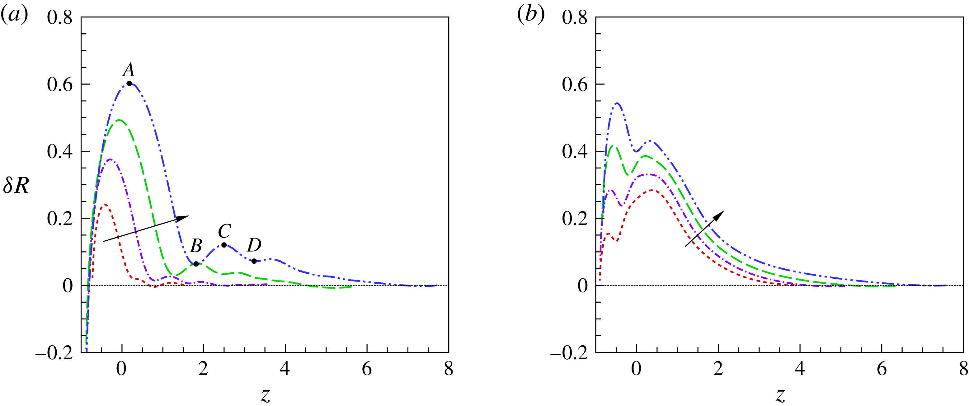
is the numerical result for the cavity wall. Figure 12 shows the vertical distribution of
 ${\it\delta}R$
at different times, in which the undisturbed surface of the liquid pool is located at
 $z=0$
while the point
 $P$
corresponds to the right end of the results. It can be seen that the magnitude of the capillary waves generally increases with time. The previous theoretical work on the time evolution of perturbations on the surface of a hollow jet in unbounded coflowing liquids suggests that the flow is absolutely unstable based on the spatio-temporal stability analysis (Ganan-Calvo Reference Ganan-Calvo2007).
In spite of the difference in the radius of the air cavity along the vertical direction, we apply the dispersion relation for a hollow jet of uniform radius to the vertical propagation of the ripples along the air cavity. In the limit of
 $Re\gg 1$
, the dimensionless dispersion relation between the perturbation wave frequency
 ${\it\omega}$
and its wavenumber
 $k$
yields (Ganan-Calvo Reference Ganan-Calvo2007; Aristoff & Bush Reference Aristoff and Bush2009)
 $$\begin{eqnarray}{\it\omega}^{2}+\frac{K_{1}(k)}{We_{j}K_{0}(k)}k(1-k^{2})=0,\end{eqnarray}$$
where
 $We_{j}={\it\rho}U^{2}a_{0}/{\it\sigma}$
and
 $a_{0}$
is the radius of the cavity;
 $K_{0}$
and
 $K_{1}$
are modified Bessel functions of the second kind of orders zero and one respectively.
Vertical propagation of the ripple arising from the impact, in term of
 ${\it\delta}R$
as a function of
 $z$
at different times. The curves correspond to the capillary waves at the same times as in figure 10, and the arrow denotes increase of the time. (a) The results for the cylinder impact and (b) the results for the sphere impact. It should be noted that the undisturbed surface of the liquid pool is set as
 $z=0$
. The bullets represent the crests and troughs of the capillary wave at
 $t=8.5$
.

Equation (3.9) can be used to theoretically estimate the wave speed by
 $c_{th}={\it\omega}/k$
, for any wavenumber
 $k$
numerically observed. The value of
 $k$
in the numerical experiments is computed by
 ${\rm\pi}/L$
, where
 $L$
is the vertical distance between the crest and its neighbouring trough on the capillary waves, e.g.
 $A$
,
 $B$
,
 $C$
and
 $D$
in figure 12. The instantaneous value of
 $a_{0}$
is set as the cavity radius at the midpoint between the crest and the trough. The wave speed in the numerical simulation,
 $c_{num}$
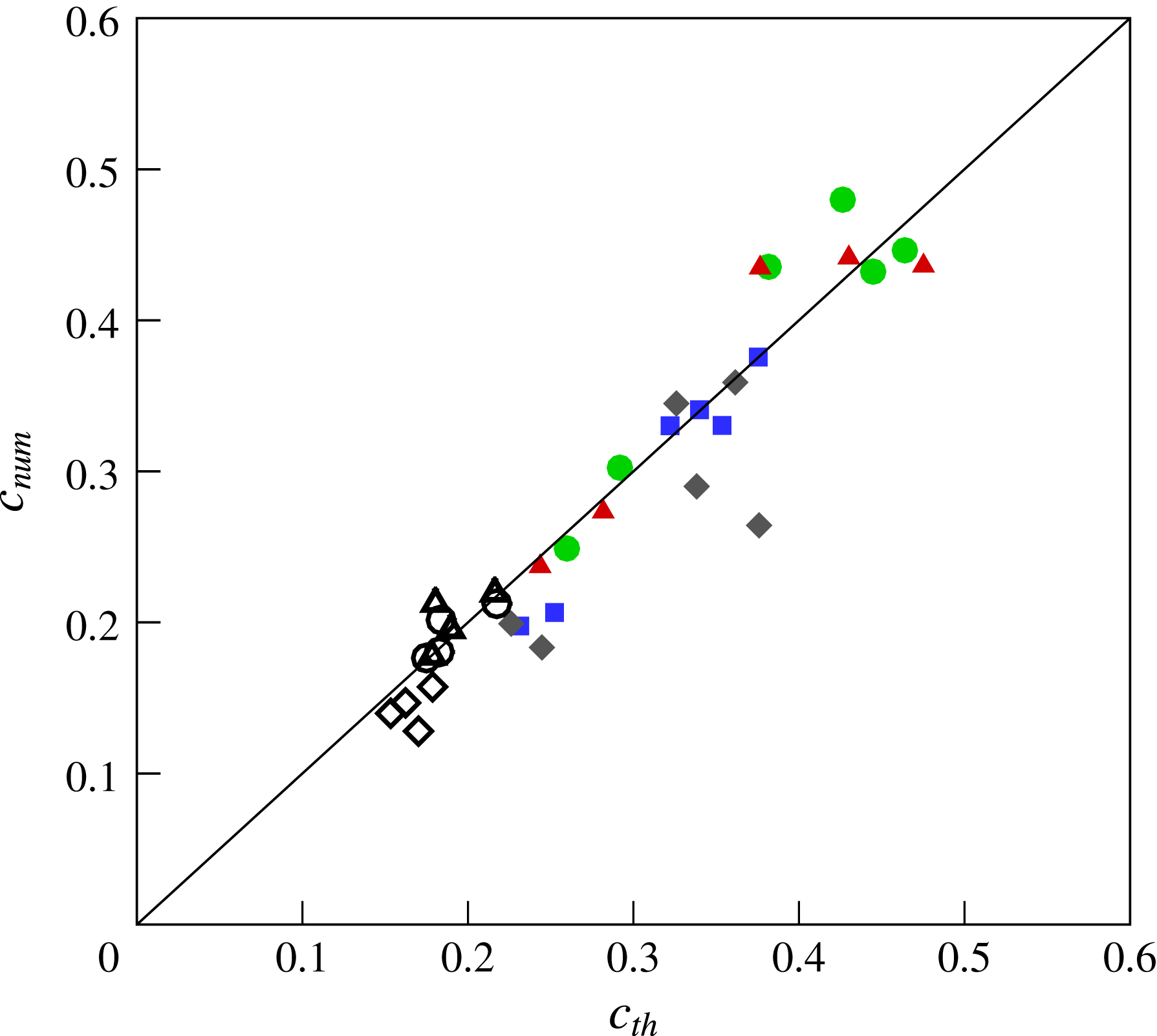
, can be obtained by interpolation at the midpoint. Figure 13 shows the comparison of the wave speed between the numerical simulation and the theoretical prediction, for various wettability and flow conditions. It is clear that a fairly good agreement has been achieved between
 $c_{th}$
and
 $c_{num}$
.
The differences in object geometry and wettability could result in different splash, and affect the magnitude of the ripples arising from the impact (Truscott et al.
Reference Truscott, Epps and Belden2014). However, the vertical propagation of these ripples along the air cavity appears to be similar: it follows the dispersion relation of the perturbation evolution on a hollow jet, with the wave speed depending only on
 $We$
. We note that an air cavity can be formed when the wave speed is larger than
 $1$
, which means that the wave would catch up with the impact object and affect the pinned CL. Since the wave speed increases with decrease of
 $We$
, it is reasonably expected that there is a low threshold for
 $We$
to obtain cavity formation.
Comparison of wave speed between the numerical simulations (
 $c_{num}$
) and the theoretical predictions (
 $c_{th}$
). The empty symbols represent the results for the sphere impact:
 ${\it\theta}_{s}=130^{\circ }$
and
 $We\,=\,400$
(▵),
 ${\it\theta}_{s}=90^{\circ }$
and
 $We\,=\,400$
(♢), and
 ${\it\theta}_{s}\,=\,90^{\circ }$
and
 $We=600$
(
 $\circ$
). The filled symbols represent the results for the cylinder impact:
 ${\it\theta}_{s}=110^{\circ }$
and
 $We=20$
(●),
 ${\it\theta}_{s}=90^{\circ }$
and
 $We=20$
(▴),
 ${\it\theta}_{s}=90^{\circ }$
and
 $We=40$
(
 $\blacklozenge$
), and
 ${\it\theta}_{s}=60^{\circ }$
and
 $We=40$
(▪).

3.5. Geometric effects on the onset of cavity formation
The geometry of the solid object makes a big difference in the critical conditions for the onset of cavity formation. Here, the onset of cavity formation is quantitatively defined by the length of the cavity besides the presence of a pinned CL: the cavity must be longer than
 $5R_{0}$
before cavity closure. Table 1 lists the critical flow conditions for a variety of object geometries with the same wettability (
 ${\it\theta}_{s}=90^{\circ }$
), including a sphere, a cylinder, a disk and two kinds of spheroids. The critical conditions are obtained by varying the impact velocity
 $U$
, so
 $Re$
changes simultaneously with
 $We$
and
 $Re\propto We^{1/2}$
. Since the viscous effect is relatively less important (
 $Re\sim O(10^{3})$
), the critical conditions for the onset of cavity formation are presented in terms of the critical Weber number,
 $We_{cr}$
. The disk can be viewed as a thin cylinder (with a thickness
 $h_{D}=0.16R_{0}$
). For the spheroids, their equatorial radii are set to
 $R_{0}$
, and the distance from the centre to the pole along the symmetry axis is set to
 $2R_{0}$
for the prolate spheroid and
 $0.6R_{0}$
for the oblate spheroid. It is interesting that among the geometries considered the disk is the easiest one for cavity formation (
 $We_{cr}=13\pm 1$
), while the prolate spheroid, the most ‘streamlined’ object here, cannot generate a cavity growing with time in the range of
 $We$
considered, i.e.
 $10\leqslant We\leqslant 350$
.
Critical Weber number for the occurrence of cavity formation,
 $We_{cr}$
, for a variety of geometries, with
 ${\it\theta}=90^{\circ }$
and
 $Re=\sqrt{We}/0.0037$
. Oblate and prolate denote the corresponding spheroids.

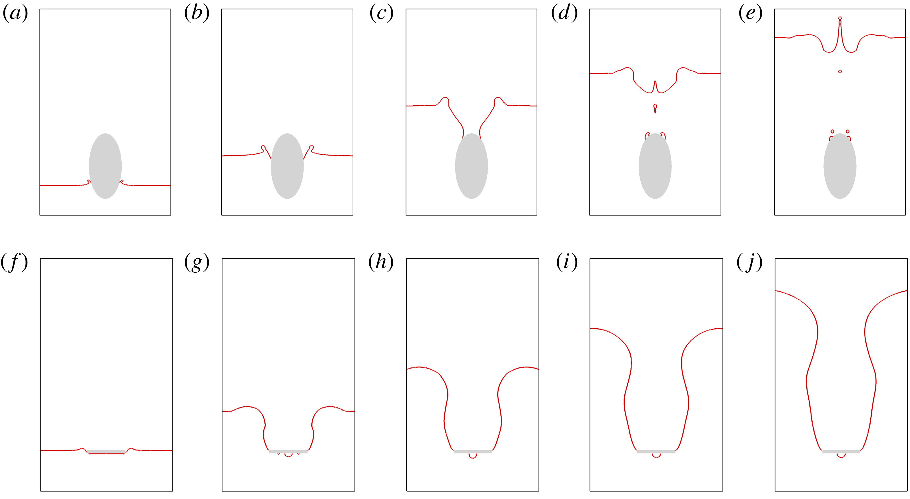
Comparison of impact dynamics between the prolate spheroid and the disk. (a–e) The prolate spheroid at
 $We=200$
,
 $Re=3800$
and
 ${\it\theta}_{s}=130^{\circ }$
, with snapshots at
 $t=0.8$
(a), 2.6 (b), 5.6 (c), 7.6 (d) and 9.6 (e). (f–j) The disk at
 $We=15$
,
 $Re=1040$
and
 ${\it\theta}_{s}=90^{\circ }$
. The snapshots start from (f) (
 $t=0.15$
) to (j) with an interval of 2.

Figure 14 shows the impact dynamics of the prolate spheroid and the disk. With a larger value of
 $We$
(
 $=200$
) than that for cavity formation in the sphere impact (
 $We=156$
in figure 3), the hydrophobic prolate spheroid (
 ${\it\theta}_{s}=130^{\circ }$
) only temporarily produces a goblet-like cavity, which ends up with a liquid jet ejecting small droplets into the air. Comparatively, the disk pulls a cavity into the water at
 $We=15$
and
 ${\it\theta}_{s}=90^{\circ }$
. We note that the CL is pinned at the upper edge of the disk. This is different from the cylinder cases, in which the CL rests either at the lower edge or on the side of the cylinder.
The big difference in critical conditions is due to the fact that the object geometry not only has a significant effect on the interface bending of the pinned meniscus, but also greatly affects the value of the low pressure in the liquid (
 $p_{l}$
in (3.2)) and the occurrence of flow separation. In single-phase flows, it is known that the more streamlined the object, the lower the maximum flow velocity (or the higher the
 $p_{l}$
based on Bernoulli’s equation), and the less possible flow separation. For an object with sharp edges like a circular cylinder, the flow velocity at the edge can be extremely large at high
 $Re$
, thereby leading to a very low pressure there (Batchelor Reference Batchelor1967). Consequently, flow separation is almost inevitable, i.e. forced flow separation. Therefore, it is reasonable to see that the objects with sharp edges require much less impact inertia (or lower
 $We_{cr}$
) to enter the regime of cavity formation than smooth objects. On the other hand, although forced flow separation occurs in the impact processes of both cylinders and disks, the effective contact-angle hysteresis at the upper edge of the disk allows the meniscus to adjust the angle that it makes with the vertical, so that the meniscus bending is effectively reduced. As a result,
 $We_{cr}$
for a disk is even less than that for a cylinder with the same wettability.
4. Conclusion
We have investigated the cavity formation in solid–liquid impact, and mainly focused on the pinning of CLs, which was found along with flow separation in the cavity formation for all of the impact objects considered. The pinned CLs were observed to be slightly above the equator of the sphere and the lower edge of the cylinder. With respective increase of
 $We$
and
 ${\it\theta}_{s}$
, the position of the pinned CL was observed to move towards the sphere equator or the lower edge of the cylinder. An analysis of the force balance at the pinned meniscus connects the wettability, inertia, effect of object geometry and interface bending with the CL position, and provides a reasonable interpretation of the numerical and experimental results. The local flow in the vicinity of the pinned CL was found to affect the global cavity dynamics, by means of changing the position and slope of the interface that connects the pinned meniscus to the interface region of radial expansion. The theoretical model based on the Rayleigh–Besant problem accurately captured the radial expansion of the cavity after the pinning of the CL. The vertical propagation of the ripples on the cavity wall was found to have a similar dispersion relation to the evolution of perturbations on a hollow jet. Finally, an object with sharp edges can cause forced flow separation and an effective contact-angle hysteresis at the edges; as a result, it is more difficult for a streamlined object to generate an air cavity than an irregular object, while the disk, with a shape exploiting the geometric effects from every aspect, requires the slowest impact velocity among all the blunt objects considered. Here, we only consider relatively less viscous liquids such as water, and we note that the liquid viscosity may also have an effect on the cavity formation; this, however, is beyond the scope of the present study.
Acknowledgements
We would like to acknowledge the support of the 100 Talents Program of the Chinese Academy of Sciences, the National Natural Science Foundation of China (grant nos 11172294, 11425210), the Chinese Academy of Sciences (grant no. KJZD-EW-J01) and the Fundamental Research Funds for the Central Universities (grant no. WK2090050025).
Supplementary movie
Supplementary movie is available at http://dx.doi.org/10.1017/jfm.2015.574.
Appendix A. Runge–Kutta methods
In the present study we use Runge–Kutta methods to numerically integrate the ordinary differential equation in the form of
 $$\begin{eqnarray}\left.\begin{array}{@{}c@{}}\displaystyle \frac{\text{d}y}{\text{d}x}=f(x,y),\\ y(x_{0})=y_{0},\end{array}\right\}\end{eqnarray}$$
where
 $f(x,y)$
is a real-valued function of
 $x$
and
 $y$
, and
 $x_{0}$
is the starting point for the numerical integration.
If a step size
 $h$
is chosen and
 $x_{k}=kh$
for
 $k=0,1,2,\ldots ,$
(A 1) can be numerically integrated step by step by using a fourth-order Runge–Kutta method. To obtain the cavity shape
 $R(z)$
based on (3.8), we use the fourth-order Runge–Kutta method twice. At the first stage, we solve
 $R_{z}$
numerically by setting
 $$\begin{eqnarray}\left.\begin{array}{@{}c@{}}x=R,\\ y=R_{z},\\ f(x,y)=(x^{-1}(1+y^{2})^{-1/2}+1.5We\,y^{2})(y(1+y^{2})^{-3/2}-We\,xy)^{-1},\end{array}\right\}\end{eqnarray}$$
and
 $x_{0}=r_{p}$
and
 $y_{0}=\tan {\it\psi}$
at the point
 $P$
(figure 6). At the second stage, we set
 $$\begin{eqnarray}\left.\begin{array}{@{}c@{}}x=z,\\ y=R,\\ f(x,y)=R_{z},\end{array}\right\}\end{eqnarray}$$
and start the numerical solution of
 $R(z)$
with
 $x_{0}=z_{p}$
and
 $y_{0}=r_{p}$
.