1 Introduction
The use of rotation to coat a solid body with a liquid film has numerous industrial applications, exemplified by spin coating in microfabrication as well as spin casting and rotational moulding at larger scales. The behaviour of a liquid film on the outer or inner surface of a rotating solid body is also of fundamental fluid mechanical interest being a seemingly simple free-surface flow problem. The liquid’s behaviour is governed by the interplay between inertia, viscosity, surface tension, gravity and rotation, which can lead to phenomena occurring on many different spatial and temporal scales, including shock-like structures (Johnson Reference Johnson1988), waves and instabilities (Phillips Reference Phillips1960) and multiple steady and unsteady solutions (Benjamin, Pritchard & Tavener Reference Benjamin, Pritchard and Tavener1993). For these reasons, the system has attracted a great deal of theoretical and experimental interest and a comprehensive recent review on the inner flow configuration (known as rimming flow) is given by Seiden & Thomas (Reference Seiden and Thomas2011) as part of a more general review of rotating-drum flows.
Following the work of Moffatt (Reference Moffatt1977) and Pukhnachev (Reference Pukhnachev1977) on the outer flow configuration (known as coating flow), the majority of previous theoretical research has focused on the case when the rotating body is a circular cylinder in the limit when the fluid film is relatively thin so that a long-wavelength analysis (lubrication theory) can be used. At leading order, the governing Navier–Stokes equations reduce to a single nonlinear partial differential equation for the film height as a function of the axial and azimuthal positions only. Many different extensions to the leading-order theory have been proposed to include the effects of surface tension (e.g. Benjamin et al. Reference Benjamin, Pritchard and Tavener1993; Ashmore, Hosoi & Stone Reference Ashmore, Hosoi and Stone2003), hydrostatic pressure (e.g. Tirumkudulu & Acrivos Reference Tirumkudulu and Acrivos2001), inertia (e.g. Kelmanson Reference Kelmanson2009; Pougatch & Frigaard Reference Pougatch and Frigaard2011) and wettability (e.g. Lin et al. Reference Lin, Rogers, Tseluiko and Thiele2016). However, as described in detail by Kelmanson (Reference Kelmanson2009) in the context of inertial effects, any asymptotic analysis is valid only in a limited region and different authors have chosen different dominant balances, preventing direct comparison of their results and leading to confusion and apparently contradictory results in the literature. Indeed, the classic mathematically convenient rescaling of the leading-order equations by Pukhnachev (Reference Pukhnachev1977) actually corresponds to non-physical parameter variations because the mass of fluid is not conserved. Thiele (Reference Thiele2011) resolved this particular problem by adopting a scaling based on gravitational drainage flow (Evans, Schwartz & Roy Reference Evans, Schwartz and Roy2004).
Early studies of coating flow were motivated by the determination of the maximum supportable weight of liquid (Moffatt Reference Moffatt1977; Hansen & Kelmanson Reference Hansen and Kelmanson1994; Kelmanson Reference Kelmanson1995), and the predictions have been confirmed experimentally by Preziosi & Joseph (Reference Preziosi and Joseph1988). More recently, however, in both rimming and coating flows attention has been focused on detailed asymptotic and numerical descriptions of the behaviour, existence and stability of solutions to the plethora of different lubrication equations (Seiden & Thomas Reference Seiden and Thomas2011). However, natural questions to ask are whether this complex behaviour is reproduced by the governing Navier–Stokes equations or ever observed in experiments.
In the classic (leading-order) lubrication model linearisation of the curvature means that the governing equation is identical for rimming and coating flow and yet, physically speaking, the systems are quite different. As the cylinder slows down, the rimming flow will always approach a steady solution in which the fluid forms a puddle at the base of the cross-section; however, a corresponding steady solution for the coating flow does not always exist, depending on the balance between surface tension, gravity and volume of fluid. Thus, the solution structure must change between these two cases, but it cannot do so within the classic model assumptions. Hence, another natural question is to ask how such a change in solution structure occurs.
In this paper, we begin to address these questions in the absence of inertia by computing steady solutions of the free-surface Stokes equations using a moving-mesh, finite-element method combined with a novel spatially adaptive pseudo-arclength continuation method. This approach allows us to examine the multiple steady solutions that can arise. To the best of our knowledge, previous numerical solutions to the Stokes equations (Peterson, Jimack & Kelmanson Reference Peterson, Jimack and Kelmanson2001; Tirumkudulu & Acrivos Reference Tirumkudulu and Acrivos2001; Benilov, Lapin & O’Brien Reference Benilov, Lapin and O’Brien2012) have always used time-stepping to approach steady states, which precludes examination of the complete steady solution structure because the unstable steady states are not accessible. We compare our results to different lubrication approximations and determine the regions of validity of each approximation. We revisit leading and first-order composite lubrication models used by previous authors and also derive a new lubrication approximation based on a gradient-dynamics approach to thin-film equations. Such a formulation was initially proposed by Mitlin (Reference Mitlin1993) for a simple lubrication model of dewetting (see also Thiele Reference Thiele2010), and was recently extended to drops and films of mixtures and suspensions on horizontal substrates in relaxational settings (Thiele, Archer & Plapp Reference Thiele, Archer and Plapp2012; Thiele, Todorova & Lopez Reference Thiele, Todorova and Lopez2013; Thiele, Archer & Pismen Reference Thiele, Archer and Pismen2016); as well as in coating processes like dip coating and Langmuir–Blodgett transfer (see review by Wilczek et al. Reference Wilczek, Tewes, Gurevich, Köpf, Chi and Thiele2015). Here we reformulate the simple lubrication model for films on a rotating cylinder as gradient dynamics with the energy computed from the lubrication approximation and then obtain a notably better model by using the exact energy instead. This model is found to exhibit good agreement with the full Stokes calculations for the widest range of parameters.
In § 2, we formulate the Stokes, § 2.1, and lubrication, § 2.2, models and then describe our numerical methods for their solution in § 3. We present the general behaviour of the Stokes system in the coating (§ 4.1) and rimming (§ 4.2) flow configurations and then discuss comparison with the simplified models in § 4.3. Finally, we draw our conclusions in § 5.
2 Mathematical model
We consider the two-dimensional flow of an incompressible Newtonian liquid film on the outside (coating) or inside (rimming) surface of a rotating cylinder. We shall assume that the effects of liquid inertia are negligible, but the effects of gravity and surface tension are not. In what follows,
 $R$
is the radius of the cylinder,
 $\unicode[STIX]{x1D714}$
is the constant angular speed of rotation about its axis,
 $\unicode[STIX]{x1D70C}$
is the density of the liquid,
 $\unicode[STIX]{x1D707}$
is its dynamic viscosity,
 $\unicode[STIX]{x1D6FE}$
is the surface tension of the air–liquid interface and
 $g$
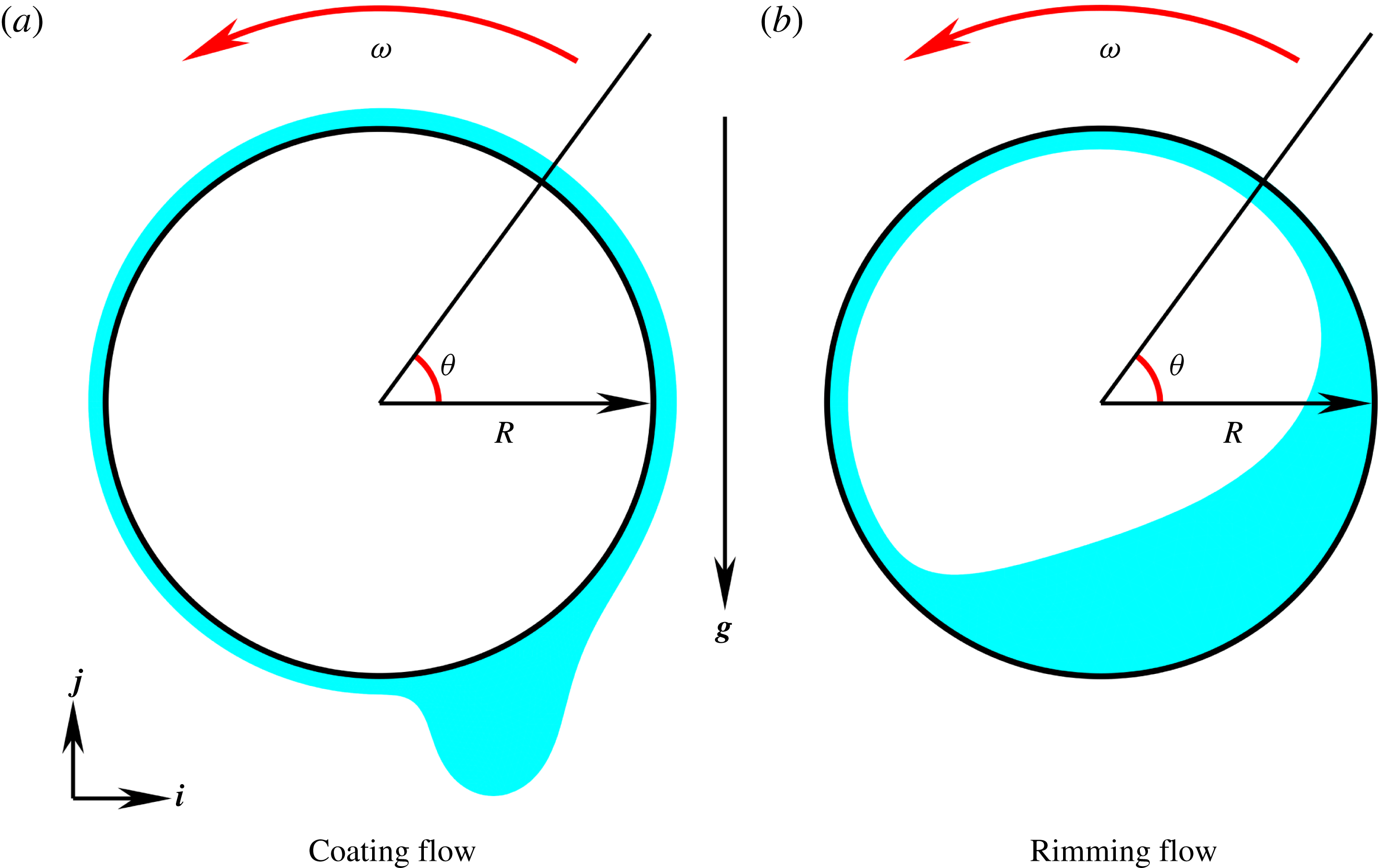
is the acceleration due to gravity. The two configurations are sketched in figure 1. We non-dimensionalise by choosing
 $R$
,
 $\unicode[STIX]{x1D70C}gR^{2}/\unicode[STIX]{x1D707}$
,
 $\unicode[STIX]{x1D707}/(\unicode[STIX]{x1D70C}gR)$
and
 $\unicode[STIX]{x1D70C}gR$
as length, velocity, time and pressure scales, respectively, which leads to parameter-free bulk (Stokes) equations, with the dimensionless parameters occurring only in the boundary conditions.
Sketches of the two flow configurations: a film of viscous liquid on the (a) outside; or (b) inside of a rotating cylinder. A gravitational field
 $\boldsymbol{g}$
acts normal to the axis of rotation and the cylinder rotates with an angular frequency
 $\unicode[STIX]{x1D714}$
. The direction of rotation as well as the polar coordinate system adopted in the lubrication models are shown in the sketches.

2.1 Stokes model
The flow of the liquid is governed by the dimensionless Stokes equations
 $$\begin{eqnarray}\displaystyle & \displaystyle \unicode[STIX]{x1D735}p=\unicode[STIX]{x1D6FB}^{2}\boldsymbol{u}-\boldsymbol{j}, & \displaystyle\end{eqnarray}$$
 $$\begin{eqnarray}\displaystyle & \displaystyle \unicode[STIX]{x1D735}\boldsymbol{\cdot }\boldsymbol{u}=0, & \displaystyle\end{eqnarray}$$
where
 $\boldsymbol{u}$
is the dimensionless velocity of the liquid,
 $p$
is the dimensionless liquid pressure and
 $\boldsymbol{j}$
is a unit vector in the vertical direction. The boundary condition at the cylinder wall is the no-slip condition,
 $$\begin{eqnarray}\boldsymbol{u}=\unicode[STIX]{x1D6FA}\boldsymbol{t}\end{eqnarray}$$
where
 $\boldsymbol{t}$
is a tangent vector to the cylinder surface in the direction of rotation and
 $$\begin{eqnarray}\unicode[STIX]{x1D6FA}=\frac{\unicode[STIX]{x1D707}\unicode[STIX]{x1D714}}{\unicode[STIX]{x1D70C}gR},\end{eqnarray}$$
is the rotation number which is the ratio between the rotational speed
 $(\unicode[STIX]{x1D714}R)$
and the chosen velocity scale
 $(\unicode[STIX]{x1D70C}gR^{2}/\unicode[STIX]{x1D707})$
. At the free surface, we impose the kinematic boundary condition
 $$\begin{eqnarray}\boldsymbol{u}\boldsymbol{\cdot }\boldsymbol{n}=\unicode[STIX]{x2202}_{t}\,\boldsymbol{x}\boldsymbol{\cdot }\boldsymbol{n},\end{eqnarray}$$
where
 $\boldsymbol{x}$
is a dimensionless position vector to a point on the free surface,
 $\boldsymbol{n}$
is the outward unit vector to the free surface and
 $t$
is the dimensionless time; and the dynamic condition
 $$\begin{eqnarray}\unicode[STIX]{x1D748}\boldsymbol{\cdot }\boldsymbol{n}=Bo^{-1}\unicode[STIX]{x1D705}\boldsymbol{n},\end{eqnarray}$$
where the surrounding gas is assumed to be inviscid and at a constant reference pressure, which we set to zero. In the dynamic boundary condition (2.6)
 $Bo$
is the Bond number,
 $$\begin{eqnarray}Bo=\frac{\unicode[STIX]{x1D70C}gR^{2}}{\unicode[STIX]{x1D6FE}},\end{eqnarray}$$
which measures the importance of gravitational forces relative to surface tension forces,
 $\unicode[STIX]{x1D705}$
is the dimensionless curvature of the free surface and
 $\unicode[STIX]{x1D748}$
, the stress tensor, is defined by
 $$\begin{eqnarray}\unicode[STIX]{x1D748}=-p\boldsymbol{I}+\left[\unicode[STIX]{x1D735}\boldsymbol{u}+\left(\unicode[STIX]{x1D735}\boldsymbol{u}\right)^{\text{T}}\right].\end{eqnarray}$$
In addition, for unsteady solutions we must also specify an initial condition
 $$\begin{eqnarray}h(\boldsymbol{x},0)=h_{0}(\boldsymbol{x}),\end{eqnarray}$$
where
 $h=h(\boldsymbol{x},t)$
is the dimensionless film thickness and
 $h_{0}$
is a given initial profile.
For steady solutions, there is no initial condition and instead the mass of liquid is prescribed, which is enforced through the integral condition
 $$\begin{eqnarray}\frac{1}{2}\oint \boldsymbol{x}\boldsymbol{\cdot }\boldsymbol{n}\,\text{d}s=2\unicode[STIX]{x03C0}\unicode[STIX]{x1D706}\left(1\pm \frac{\unicode[STIX]{x1D706}}{2}\right),\end{eqnarray}$$
where the line integral is taken along the free-surface boundary,
 $\unicode[STIX]{x1D706}$
is the aspect ratio,
 $$\begin{eqnarray}\unicode[STIX]{x1D706}=\frac{D}{R},\end{eqnarray}$$
and
 $D$
is the nominal average dimensional film thickness. Note that
 $2\unicode[STIX]{x03C0}\unicode[STIX]{x1D706}(1\pm \unicode[STIX]{x1D706}/2)$
is the dimensionless volume per unit length of a uniform film of thickness
 $D$
on the outer (positive sign) or inner (negative sign) wall of the cylinder.
2.2 Lubrication model
We adopt a dimensionless polar coordinate system
 $(r,\unicode[STIX]{x1D703})$
with origin at the centre of the cylinder and
 $\unicode[STIX]{x1D703}$
measured upward from the horizontal, see figure 1. The free surface is then given by
 $r=1\pm h$
, where
 $h=h(\unicode[STIX]{x1D703},t)$
is, as stated before, the dimensionless film thickness and the upper and lower signs correspond, in that order, to the coating and rimming problems. After Evans et al. (Reference Evans, Schwartz and Roy2004), we rescale the system via
 $$\begin{eqnarray}\displaystyle \left.\begin{array}{@{}c@{}}\displaystyle u=\unicode[STIX]{x1D706}^{3}u^{\ast },\quad v=\unicode[STIX]{x1D706}^{2}v^{\ast },\quad t=t^{\ast }/\unicode[STIX]{x1D706}^{2},\\ \displaystyle p=p^{\ast },\quad h=\unicode[STIX]{x1D706}h^{\ast },\quad r=1\pm \unicode[STIX]{x1D706}y^{\ast },\quad \unicode[STIX]{x1D705}=\unicode[STIX]{x1D706}\unicode[STIX]{x1D705}^{\ast },\end{array}\right\} & & \displaystyle\end{eqnarray}$$
where
 $u$
and
 $v$
are the radial and azimuthal components of the velocity and the variables marked by the asterisks are the scaled variables. Assuming
 $\unicode[STIX]{x1D706}\ll 1$
, lubrication theory can be employed to reduce the governing equations (2.1)–(2.6) to the following nonlinear evolution equation for the film height (asterisks omitted)
 $$\begin{eqnarray}\unicode[STIX]{x2202}_{t}h+\unicode[STIX]{x2202}_{\unicode[STIX]{x1D703}}\left[\unicode[STIX]{x1D6FA}_{\unicode[STIX]{x1D706}}h-\frac{h^{3}}{3}\cos \unicode[STIX]{x1D703}+{Bo_{\unicode[STIX]{x1D706}}}^{-1}\frac{h^{3}}{3}\left(\unicode[STIX]{x2202}_{\unicode[STIX]{x1D703}}^{3}h+\unicode[STIX]{x2202}_{\unicode[STIX]{x1D703}}h\right)\right]=0\end{eqnarray}$$
(Pukhnachev Reference Pukhnachev1977; Reisfeld & Bankoff Reference Reisfeld and Bankoff1992), where
 $\unicode[STIX]{x1D6FA}_{\unicode[STIX]{x1D706}}$
is a modified rotation number,
 $$\begin{eqnarray}\unicode[STIX]{x1D6FA}_{\unicode[STIX]{x1D706}}=\frac{\unicode[STIX]{x1D6FA}}{\unicode[STIX]{x1D706}^{2}}=\frac{\unicode[STIX]{x1D707}\unicode[STIX]{x1D714}R}{\unicode[STIX]{x1D70C}gD^{2}},\end{eqnarray}$$
and
 $Bo_{\unicode[STIX]{x1D706}}$
is a modified Bond number,
 $$\begin{eqnarray}Bo_{\unicode[STIX]{x1D706}}=\frac{Bo}{\unicode[STIX]{x1D706}}=\frac{\unicode[STIX]{x1D70C}gR^{3}}{\unicode[STIX]{x1D6FE}D}.\end{eqnarray}$$
The rescalings have specifically been chosen so that the rotation and gravitational terms occur at leading order in
 $\unicode[STIX]{x1D706}$
in the governing equations. Note that
 $O(\unicode[STIX]{x1D706}\unicode[STIX]{x1D6FA}_{\unicode[STIX]{x1D706}},\unicode[STIX]{x1D706}Bo_{\unicode[STIX]{x1D706}}^{-1},\unicode[STIX]{x1D706})$
terms have been omitted. In the steady case,
 $\unicode[STIX]{x2202}_{t}h=0$
and thus equation (2.13) can be immediately integrated to give the flux equation
 $$\begin{eqnarray}q=\unicode[STIX]{x1D6FA}_{\unicode[STIX]{x1D706}}h-\frac{h^{3}}{3}\cos \unicode[STIX]{x1D703}+{Bo_{\unicode[STIX]{x1D706}}}^{-1}\frac{h^{3}}{3}(\unicode[STIX]{x2202}_{\unicode[STIX]{x1D703}}^{3}h+\unicode[STIX]{x2202}_{\unicode[STIX]{x1D703}}h),\end{eqnarray}$$
where the constant of integration,
 $q$
, represents the unknown (dimensionless) flux required to satisfy the mass conservation condition which, to leading order in
 $\unicode[STIX]{x1D706}$
, is given by
 $$\begin{eqnarray}\int _{0}^{2\unicode[STIX]{x03C0}}h\,\text{d}\unicode[STIX]{x1D703}=2\unicode[STIX]{x03C0}.\end{eqnarray}$$
The first, second and third terms in the right-hand side of equation (2.16) represent, respectively, the rotational viscous drag, gravity and surface tension leading-order effects. Note that equations (2.16) and (2.17) are identical for rimming and coating flows and we shall term this the standard lubrication model (SLM). The SLM has been widely studied and it is the most commonly used lubrication model to describe the motion of a viscous film on the surface of a rotating cylinder (e.g. Pukhnachev Reference Pukhnachev1977; Reisfeld & Bankoff Reference Reisfeld and Bankoff1992; Hinch & Kelmanson Reference Hinch and Kelmanson2003; Karabut Reference Karabut2007; Benilov, Benilov & Kopteva Reference Benilov, Benilov and Kopteva2008; Badali et al. Reference Badali, Chugunova, Pelinovsky and Pollack2011; Thiele Reference Thiele2011).
More recently Evans et al. (Reference Evans, Schwartz and Roy2004) and Benilov & O’Brien (Reference Benilov and O’Brien2005) derived the following flux equation
 $$\begin{eqnarray}\displaystyle q & = & \displaystyle \unicode[STIX]{x1D6FA}_{\unicode[STIX]{x1D706}}h-\frac{h^{3}}{3}\cos \unicode[STIX]{x1D703}+{Bo_{\unicode[STIX]{x1D706}}}^{-1}\frac{h^{3}}{3}\left(\unicode[STIX]{x2202}_{\unicode[STIX]{x1D703}}^{3}h+\unicode[STIX]{x2202}_{\unicode[STIX]{x1D703}}h\right)\nonumber\\ \displaystyle & & \displaystyle \pm \,\unicode[STIX]{x1D706}\left(\unicode[STIX]{x1D6FA}_{\unicode[STIX]{x1D706}}\frac{h^{2}}{2}-\frac{h^{4}}{2}\cos \unicode[STIX]{x1D703}-\frac{h^{3}}{3}\unicode[STIX]{x2202}_{\unicode[STIX]{x1D703}}h\sin \unicode[STIX]{x1D703}\right),\end{eqnarray}$$
or, written alternatively,
 $$\begin{eqnarray}\displaystyle q & = & \displaystyle \unicode[STIX]{x1D6FA}_{\unicode[STIX]{x1D706}}h\left(1\pm \unicode[STIX]{x1D706}\frac{h}{2}\right)+{Bo_{\unicode[STIX]{x1D706}}}^{-1}\frac{h^{3}}{3}\left(\unicode[STIX]{x2202}_{\unicode[STIX]{x1D703}}^{3}h+\unicode[STIX]{x2202}_{\unicode[STIX]{x1D703}}h\right)\nonumber\\ \displaystyle & & \displaystyle -\,\frac{h^{3}}{3}\left[\left(1\pm \unicode[STIX]{x1D706}\frac{h}{2}\right)\cos \unicode[STIX]{x1D703}\pm \unicode[STIX]{x1D706}\unicode[STIX]{x2202}_{\unicode[STIX]{x1D703}}(h\sin \unicode[STIX]{x1D703})\right],\end{eqnarray}$$
where now
 $O(\unicode[STIX]{x1D706}^{2}\unicode[STIX]{x1D6FA}_{\unicode[STIX]{x1D706}},\unicode[STIX]{x1D706}Bo_{\unicode[STIX]{x1D706}}^{-1},\unicode[STIX]{x1D706}^{2})$
terms have been omitted. Note that the hydrostatic pressure is represented by the final two terms at
 $O(\unicode[STIX]{x1D706})$
in (2.18). Also, it is worth mentioning that in the asymptotic derivation of this flux equation, both works assumed that
 $Bo_{\unicode[STIX]{x1D706}}$
is
 $O(\unicode[STIX]{x1D706})$
, in contrast to Pukhnachev (Reference Pukhnachev1977), Reisfeld & Bankoff (Reference Reisfeld and Bankoff1992), who assumed that
 $Bo_{\unicode[STIX]{x1D706}}$
is
 $O(1)$
in their derivations. Equation (2.18) does distinguish the rimming- and coating-flow cases and, moreover, including terms of
 $O(\unicode[STIX]{x1D706})$
ensures exact mass conservation via the integral constraint
 $$\begin{eqnarray}\int _{0}^{2\unicode[STIX]{x03C0}}\left(h\pm \unicode[STIX]{x1D706}\frac{h^{2}}{2}\right)\,\text{d}\unicode[STIX]{x1D703}=2\unicode[STIX]{x03C0}\left(1\pm \frac{\unicode[STIX]{x1D706}}{2}\right),\end{eqnarray}$$
unlike (2.17). We shall term equations (2.18) and (2.20) the extended lubrication model (ELM). The ELM has been mostly used to investigate the stability of rimming flows on rotating cylinders when inertial effects (which here are neglected) are taken into account (e.g. Benilov & O’Brien Reference Benilov and O’Brien2005; Pougatch & Frigaard Reference Pougatch and Frigaard2011).
In appendix B, we use a variational approach to derive the following model, which we believe has not been studied before,
 $$\begin{eqnarray}q=\unicode[STIX]{x1D6FA}_{\unicode[STIX]{x1D706}}h-\frac{h^{3}}{3}\unicode[STIX]{x2202}_{\unicode[STIX]{x1D703}}\left[-Bo_{\unicode[STIX]{x1D706}}^{-1}\unicode[STIX]{x1D705}+(1\pm \unicode[STIX]{x1D706}h)\sin \unicode[STIX]{x1D703}\right].\end{eqnarray}$$
Note that to leading order, equation (2.21) is equivalent to equation (2.13). The previous equation can be cast into gradient-dynamics form (in the frame moving with the cylinder surface) as
 $$\begin{eqnarray}q=\unicode[STIX]{x1D6FA}_{\unicode[STIX]{x1D706}}h-Q\unicode[STIX]{x2202}_{\unicode[STIX]{x1D703}}\left[\left(1\pm \unicode[STIX]{x1D706}h\right)^{-1}\frac{\unicode[STIX]{x1D6FF}F}{\unicode[STIX]{x1D6FF}h}\right],\end{eqnarray}$$
where
 $Q=Q(h)=h^{3}/3$
is known as the mobility factor and
 $\unicode[STIX]{x1D6FF}F/\unicode[STIX]{x1D6FF}h$
represents the variational derivative of the dimensionless free energy
 $F=F[h]=\int Bo_{\unicode[STIX]{x1D706}}^{-1}\,\text{d}s+\iint r\sin \unicode[STIX]{x1D703}\,\text{d}A$
, consisting of surface energy (surface tension) and potential energy (gravitational) terms.
In this model, unlike in the previous two, we do not use any approximation for the curvature but use the full expression
 $$\begin{eqnarray}\unicode[STIX]{x1D705}={\displaystyle \frac{\mp \unicode[STIX]{x1D706}^{-1}(1\pm \unicode[STIX]{x1D706}h)^{2}\mp 2\unicode[STIX]{x1D706}\left(\unicode[STIX]{x2202}_{\unicode[STIX]{x1D703}}h\right)^{2}+(1\pm \unicode[STIX]{x1D706}h)\unicode[STIX]{x2202}_{\unicode[STIX]{x1D703}}^{2}h}{\left[(1\pm \unicode[STIX]{x1D706}h)^{2}+\unicode[STIX]{x1D706}^{2}(\unicode[STIX]{x2202}_{\unicode[STIX]{x1D703}}h)^{2}\right]^{3/2}}}.\end{eqnarray}$$
Consequently, the full expression for the free energy
 $F[h]$
is also retained. We shall term equations (2.22) and (2.20) the variational lubrication model (VLM). Using the exact curvature has been found to improve the accuracy of lubrication models in a number of applications, including liquid-film breakup (Gauglitz & Radke Reference Gauglitz and Radke1988) and models of airway closure (Heil & White Reference Heil and White2002). The gradient dynamics viewpoint allows us to reinterpret this well-known ‘exact-curvature trick’ as being a means to ensure that the free energy is exact, with only the mobility being approximate. In other words, static equilibria will be correctly represented, but dynamic effects are approximated. Note that this approach is not ‘rational’ in a strict asymptotic sense because the neglected terms are not all of the same order in
 $\unicode[STIX]{x1D706}$
. Nonetheless, the resulting equations require only a modest increase in computational effort and can yield significantly improved results. We remark that, of course, when working at a finite value of the small parameter, the fact that an approximation is formally asymptotic is in itself no guarantee of a good approximation. In systems where the results are sensitive to energy and mass conservation then the approach advocated here may also prove to be more accurate at finite values than a formal asymptotic analysis.
We note that the lubrication models presented in this section are based not only on the assumption that
 $\unicode[STIX]{x1D706}\ll 1$
, but also on the more restrictive assumption that the Stokes approximation is valid. As shown by Evans et al. (Reference Evans, Schwartz and Roy2004), neglect of the inertial terms in the lubrication approximation corresponds to neglect of terms of
 $O(\unicode[STIX]{x1D706}^{2}Re)$
, where
 $$\begin{eqnarray}Re=\frac{\unicode[STIX]{x1D70C}^{2}gD^{2}R}{\unicode[STIX]{x1D707}^{2}}\end{eqnarray}$$
is the Reynolds number. Thus, inertial effects will not enter the SLM or ELM, provided that
 $Re\ll 1$
, consistent with the assumption that the Stokes equations are valid. Evans et al. (Reference Evans, Schwartz and Roy2004) also confirmed the validity of the Stokes approximation for the experimental results obtained by Yih & Kingman (Reference Yih and Kingman1960) and also for the simple qualitative experiment reported by Moffatt (Reference Moffatt1977), for which
 $O(\unicode[STIX]{x1D706}^{2}Re)\sim 10^{-3}$
.
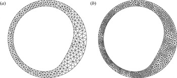
Examples of triangular meshes generated in the rimming-flow configuration at
 $\unicode[STIX]{x1D706}=0.2$
,
 $\unicode[STIX]{x1D6FA}_{\unicode[STIX]{x1D706}}=1$
and
 $Bo_{\unicode[STIX]{x1D706}}=100$
: (b) was generated by refining (a).

3 Numerical methods
3.1 Stokes model
We solve the governing equations (2.1)–(2.9) using a finite-element method (FEM) implemented within the open-source software oomph-lib (Heil & Hazel Reference Heil, Hazel, Bungartz and Schäfer2006) and previously described in Hazel et al. (Reference Hazel, Heil, Waters and Oliver2012). Briefly, we employ a standard two-dimensional Cartesian coordinate system
 $(x,y)$
and the a priori unknown liquid domain is discretised using
 $P_{2}P_{1}$
(Taylor–Hood) triangular elements (see e.g. Gresho & Sani Reference Gresho and Sani1998). These LBB (Ladyzhenskaya–Babuska–Brezzi) stable elements employ a continuous piecewise quadratic approximation for the velocity components and a continuous piecewise linear approximation for the pressure field. An initial mesh is created using Triangle (Shewchuk Reference Shewchuk and Lin1996) and during the computations, the nodal positions are updated by treating the mesh as a pseudo-elastic solid body. The unknown nodal positions are determined by solving the equations of large-displacement elasticity, subject to the kinematic boundary condition (2.5), imposed using Lagrange-multiplier-like variables to apply a normal force on the pseudo-solid along the interface. The dynamic boundary condition (2.6) is directly incorporated into the weak form of the Navier–Stokes equations, and we simplify the curvature term by the surface divergence theorem. The flow is enclosed, which means that a reference pressure must be specified and we choose the external pressure to be zero and use the mass conservation constraint (2.9) to determine a single selected pressure value within the liquid domain. The system is linearised using a global Newton method and solved using a direct solver.
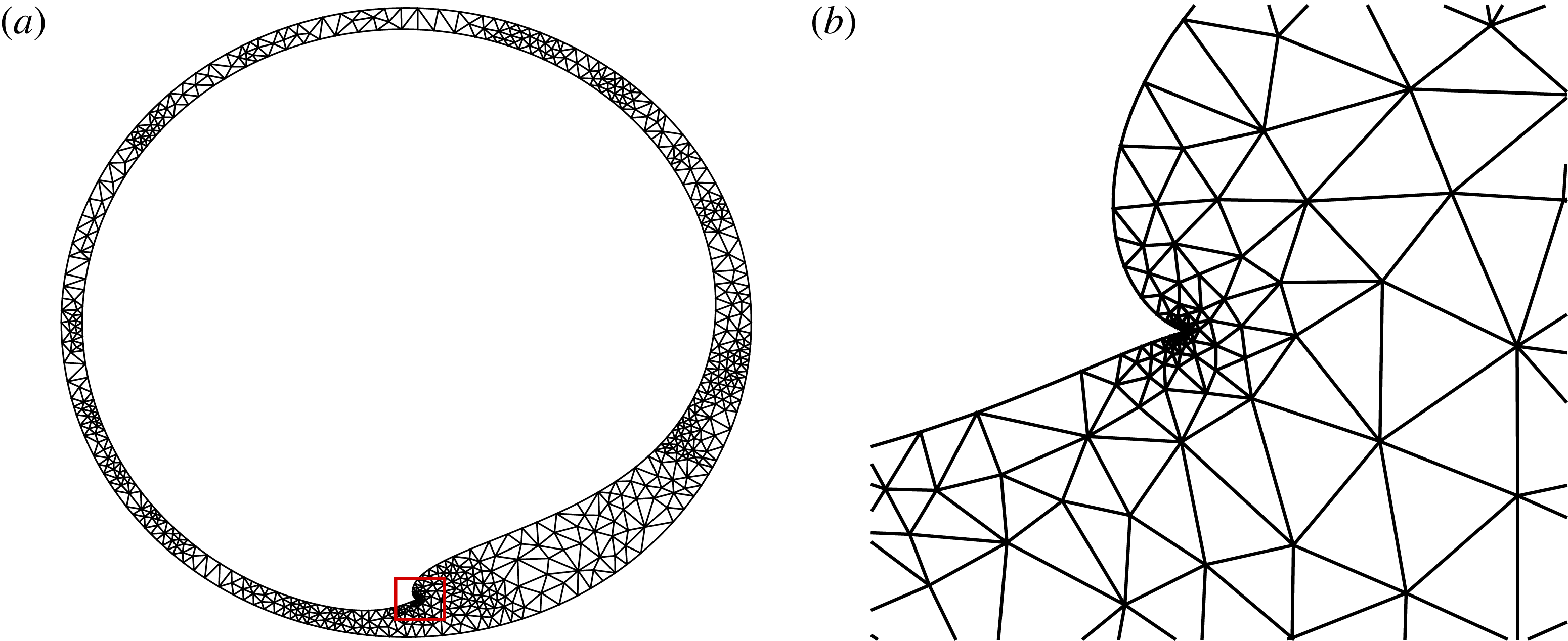
During parameter variations, the liquid domain can change morphology significantly and the domain is remeshed to avoid the elemental distortion and maintain accuracy of the solution; figure 2 shows the same solution for two different mesh resolutions. The previous solution is projected onto the new mesh and used as the initial guess to the Newton method. Elemental sizes in the new mesh are based on error estimates obtained from the ZZ flux-recovery error estimator (Zienkiewicz & Zhu Reference Zienkiewicz and Zhu1992). We use pseudo-arclength continuation (Kuznetsov Reference Kuznetsov2010; Dijkstra et al.
Reference Dijkstra, Wubs, Cliffe, Doedel, Dragomirescu, Eckhardt, Gelfgat, Hazel, Lucarini and Salinger2014) to follow the solution branches round limit points that can develop. The combination of spatial adaptivity and continuation in free-surface problems is a novel numerical technique and requires projection of auxiliary variables, specifically an estimate of the tangent vector and previous converged solution, onto the new mesh. Typically between 2000 and 6000 elements are used and we have confirmed that repeating computations with smaller error tolerances, and therefore increasing the numbers of elements does not affect the results to graphical accuracy, as shown by calculations at two different mesh resolutions for
 $Bo_{\unicode[STIX]{x1D706}}=2000$
in figure 7. In addition, we have also confirmed that the results of our Stokes calculations agree with those of previous authors (Peterson et al.
Reference Peterson, Jimack and Kelmanson2001; Tirumkudulu & Acrivos Reference Tirumkudulu and Acrivos2001).
3.2 Lubrication model
We use a similar finite-element approach to solve the lubrication models developed in § 2.2 also implemented within oomph-lib. All three models can be written in the form
 $$\begin{eqnarray}\unicode[STIX]{x2202}_{\unicode[STIX]{x1D703}}\left[{\mathcal{A}}\unicode[STIX]{x1D6FA}_{\unicode[STIX]{x1D706}}h+\frac{h^{3}}{3}(Bo_{\unicode[STIX]{x1D706}}\unicode[STIX]{x2202}_{\unicode[STIX]{x1D703}}{\mathcal{B}}-{\mathcal{C}})\right]=0,\end{eqnarray}$$
where
 $$\begin{eqnarray}{\mathcal{A}}={\mathcal{A}}(h)=\left\{\begin{array}{@{}ll@{}}1,\quad & \text{in the SLM and VLM},\\ 1+\unicode[STIX]{x1D6FC}{\displaystyle \frac{h}{2}},\quad & \text{in the ELM},\end{array}\right.\end{eqnarray}$$
with
 $$\begin{eqnarray}\displaystyle & \displaystyle \unicode[STIX]{x1D6FC}=\left\{\begin{array}{@{}ll@{}}\unicode[STIX]{x1D706},\quad & \text{in the coating case,}\\ -\unicode[STIX]{x1D706},\quad & \text{in the rimming case,}\end{array}\right. & \displaystyle\end{eqnarray}$$
 $$\begin{eqnarray}\displaystyle & \displaystyle {\mathcal{B}}={\mathcal{B}}(h,\unicode[STIX]{x2202}_{\unicode[STIX]{x1D703}}h,\unicode[STIX]{x2202}_{\unicode[STIX]{x1D703}}^{2}h)=\left\{\begin{array}{@{}ll@{}}-\unicode[STIX]{x1D6FC}^{-1}+\unicode[STIX]{x2202}_{\unicode[STIX]{x1D703}}^{2}h+h,\quad & \text{in the SLM and ELM,}\\ \unicode[STIX]{x1D705},\quad & \text{in the VLM,}\end{array}\right. & \displaystyle\end{eqnarray}$$
 $$\begin{eqnarray}\displaystyle & \displaystyle {\mathcal{C}}={\mathcal{C}}(h,\unicode[STIX]{x2202}_{\unicode[STIX]{x1D703}}h,\unicode[STIX]{x1D703})=\left\{\begin{array}{@{}ll@{}}\cos \unicode[STIX]{x1D703},\quad & \text{in the SLM,}\\ {\mathcal{A}}\cos \unicode[STIX]{x1D703}+\unicode[STIX]{x1D6FC}\unicode[STIX]{x2202}_{\unicode[STIX]{x1D703}}(h\sin \unicode[STIX]{x1D703}),\quad & \text{in the ELM and VLM.}\end{array}\right. & \displaystyle\end{eqnarray}$$
We then use the substitutions
 $v_{1}=h$
and
 $v_{2}={\mathcal{B}}$
to transform the equation (3.1) into a system of two coupled second-order ordinary differential equations:
 $$\begin{eqnarray}\left.\begin{array}{@{}c@{}}\unicode[STIX]{x2202}_{\unicode[STIX]{x1D703}}\left[{\mathcal{A}}\unicode[STIX]{x1D6FA}_{\unicode[STIX]{x1D706}}v_{1}+{\displaystyle \frac{v_{1}^{3}}{3}}(Bo_{\unicode[STIX]{x1D706}}\unicode[STIX]{x2202}_{\unicode[STIX]{x1D703}}v_{2}-{\mathcal{C}})\right]=0,\\ {\mathcal{B}}-v_{2}=0.\end{array}\right\}\end{eqnarray}$$
These equations are converted into weak form and discretised by standard Lagrange finite elements with quadratic approximation for both variables
 $v_{1}$
and
 $v_{2}$
. The equations are solved under the periodic boundary conditions
 $v_{1}(\unicode[STIX]{x1D703})=v_{1}(2\unicode[STIX]{x03C0}+\unicode[STIX]{x1D703})$
and
 $v_{2}(\unicode[STIX]{x1D703})=v_{2}(2\unicode[STIX]{x03C0}+\unicode[STIX]{x1D703})$
and we use the mass conservation constraint, i.e. equation (2.17) in the SLM or equation (2.20) in the ELM and in the VLM, to determine a single selected height value within the domain. The domain is simply
 $\unicode[STIX]{x1D703}\in [0,2\unicode[STIX]{x03C0}]$
which is initially divided into a uniform mesh and we use spatial adaptivity guided by a Z2 error estimator to refine the solution in regions of rapid variation. We again use pseudo-arclength continuation to follow the solution around limit points. The system of equations is linearised using Newton’s method and solved by a direct linear solver. Typically 300 elements are required and solutions were validated by comparison with the Stokes flow solutions in the expected region of validity; and by recomputing selected cases with finer error tolerances.
4 Results
The system is governed by the three control parameters
 $\unicode[STIX]{x1D6FA}$
,
 $Bo$
and
 $\unicode[STIX]{x1D706}$
, which can be interpreted as the rotation rate of the cylinder; strength of gravity relative to surface tension; and mass of liquid respectively. Note that other authors have used different combinations of variables as their control parameters, but there are always three parameters if surface tension effects are included in the model. Our choice of parameters is motivated from physical experiments: for a given experimental set-up,
 $Bo$
is likely to remain fixed, but the rotation rate
 $\unicode[STIX]{x1D6FA}$
and the mass of fluid
 $\unicode[STIX]{x1D706}$
can be adjusted easily. In the following sections we present all results in terms of the parameters in the lubrication theory scaling, but, unless stated otherwise, we keep the nominal film thickness fixed at
 $\unicode[STIX]{x1D706}=0.1$
, so that
 $Bo=0.1Bo_{\unicode[STIX]{x1D706}}$
and
 $\unicode[STIX]{x1D6FA}=0.01\unicode[STIX]{x1D6FA}_{\unicode[STIX]{x1D706}}$
maintain the same proportions of the unscaled values. We present parameter studies in which the Bond number is fixed, but the rotation parameter is varied, corresponding to experiments in which the physical rotation rate is varied, but the physical properties of the liquid remain constant. We first examine the general behaviour of the coating and rimming systems under Stokes flow, before turning our attention to the validity and quality of the various lubrication approximations.
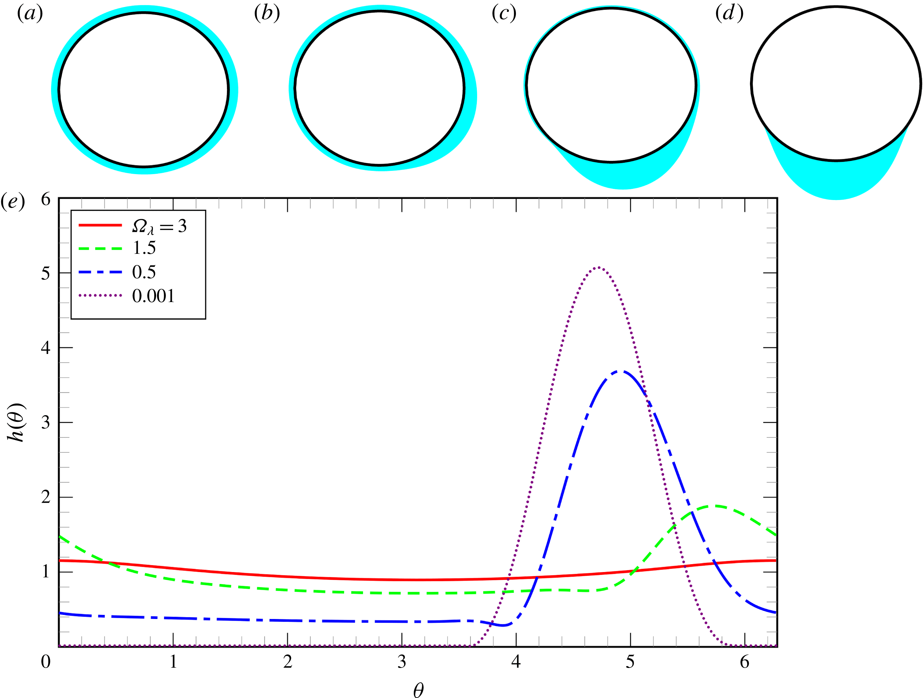
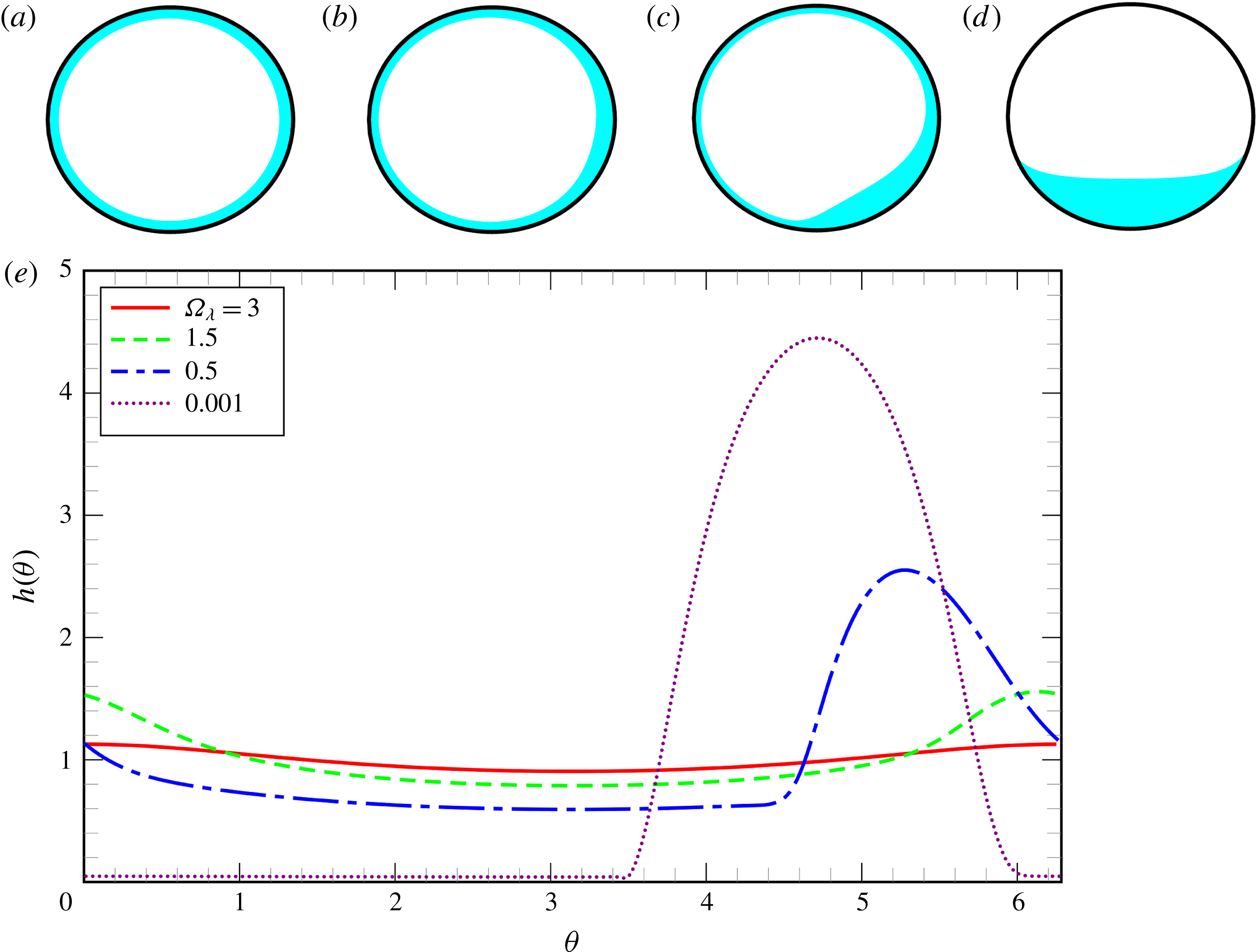
Example of coating-flow profiles obtained from the numerical solution of the Stokes equations for
 $\unicode[STIX]{x1D706}=0.1$
and
 $Bo_{\unicode[STIX]{x1D706}}=20$
for: (a)
 $\unicode[STIX]{x1D6FA}_{\unicode[STIX]{x1D706}}=3$
; (b)
 $\unicode[STIX]{x1D6FA}_{\unicode[STIX]{x1D706}}=1.5$
; (c)
 $\unicode[STIX]{x1D6FA}_{\unicode[STIX]{x1D706}}=0.5$
; (d)
 $\unicode[STIX]{x1D6FA}_{\unicode[STIX]{x1D706}}=0.001$
. The upper panels illustrate the film profiles on the cylinder while the lower panel shows the same profiles as functions
 $h(\unicode[STIX]{x1D703})$
.

4.1 Coating flow
Figure 3 presents film profiles at different rotation rates for
 $Bo_{\unicode[STIX]{x1D706}}=20$
. At high rotation rates (
 $\unicode[STIX]{x1D6FA}_{\unicode[STIX]{x1D706}}=3$
, figure 3
a) the film is approximately symmetric about the horizontal midplane of the cylinder with a maximum thickness at
 $\unicode[STIX]{x1D703}\approx 0$
(where gravitational drainage acts against rotation) and minimum at
 $\unicode[STIX]{x1D703}\approx \unicode[STIX]{x03C0}$
(where gravitational drainage acts with the rotation). As
 $\unicode[STIX]{x1D6FA}$
increases further these extrema decrease in amplitude and the uniform-film limit is approached. Conversely, as the rotation rate decreases gravitational drainage increases and the maximum film thickness also increases and moves against the direction of rotation towards the base of the cylinder,
 $\unicode[STIX]{x1D703}=3\unicode[STIX]{x03C0}/2$
. As
 $\unicode[STIX]{x1D6FA}\rightarrow 0$
, the fluid adopts a pendant-drop configuration. We have not computed the case where the cylinder is static (
 $\unicode[STIX]{x1D6FA}=0$
), because our numerical simulations assume continuous coating and must therefore mesh the vanishingly thin films on the upper surface of the cylinder, which becomes prohibitively expensive. At
 $\unicode[STIX]{x1D6FA}=0.001$
, the film thickness is less than
 $1.6\times 10^{-2}R$
outside the drop region.
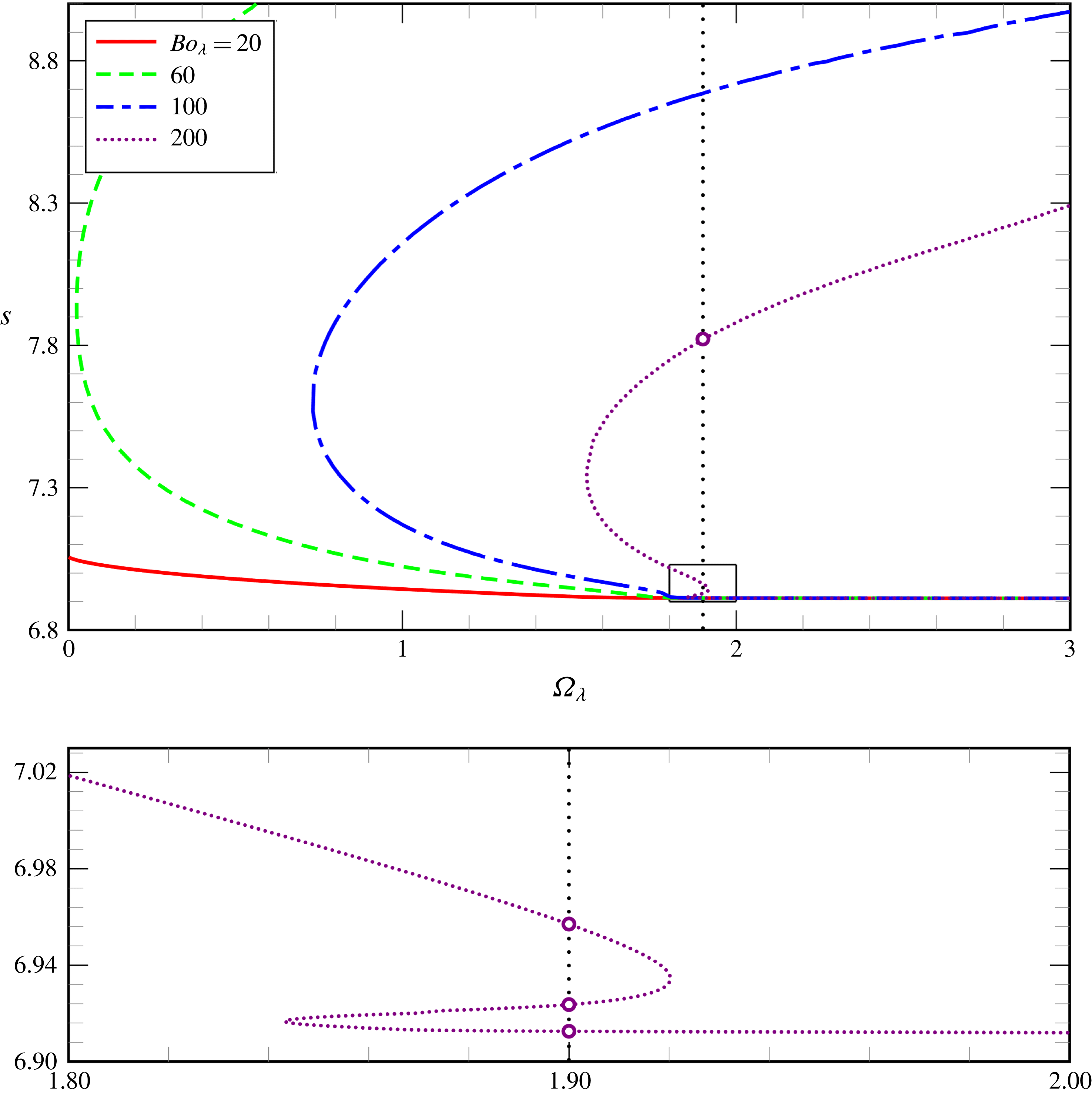
Fluid perimeter
 $s$
for coating flow as a function of the rotation number
 $\unicode[STIX]{x1D6FA}_{\unicode[STIX]{x1D706}}$
for different Bond numbers
 $Bo_{\unicode[STIX]{x1D706}}$
, as obtained from the numerical solution of the Stokes equations for
 $\unicode[STIX]{x1D706}=0.1$
. The lower panel is an expanded view of the region marked by the box in the upper panel for the case
 $Bo_{\unicode[STIX]{x1D706}}=200$
only. The multiple solutions at
 $\unicode[STIX]{x1D6FA}_{\unicode[STIX]{x1D706}}=1.9$
(marked by circles on the vertical dotted line) are shown in figure 5.

Example of a coating flow with multiple steady states as obtained from the numerical solution of the Stokes equations for
 $\unicode[STIX]{x1D706}=0.1$
,
 $Bo_{\unicode[STIX]{x1D706}}=200$
and
 $\unicode[STIX]{x1D6FA}_{\unicode[STIX]{x1D706}}=1.9$
: (a)
 $s\approx 6.91$
; (b)
 $s\approx 6.93$
; (c)
 $s\approx 6.96$
; (d)
 $s\approx 7.82$
. The upper panels illustrate the film profiles on the cylinder while the lower panel shows the same profiles as functions
 $h(\unicode[STIX]{x1D703})$
.

Rather than including a large number of film profiles, we summarise the steady solutions for coating flow in figure 4 by plotting length of the liquid’s outer perimeter as a function of rotation rate
 $\unicode[STIX]{x1D6FA}_{\unicode[STIX]{x1D706}}$
for different values of
 $Bo_{\unicode[STIX]{x1D706}}$
. The perimeter is a global measure of the solution that has the advantage, compared to the
 $L^{2}$
norm of
 $h(\unicode[STIX]{x1D703})$
used by Thiele (Reference Thiele2011) and others that it remains well defined in cases when the surface becomes multivalued at fixed
 $\unicode[STIX]{x1D703}$
. When the Bond number is small (
 $Bo_{\unicode[STIX]{x1D706}}=20$
), the surface tension effects are dominant and only one solution exists for each value of
 $\unicode[STIX]{x1D6FA}_{\unicode[STIX]{x1D706}}$
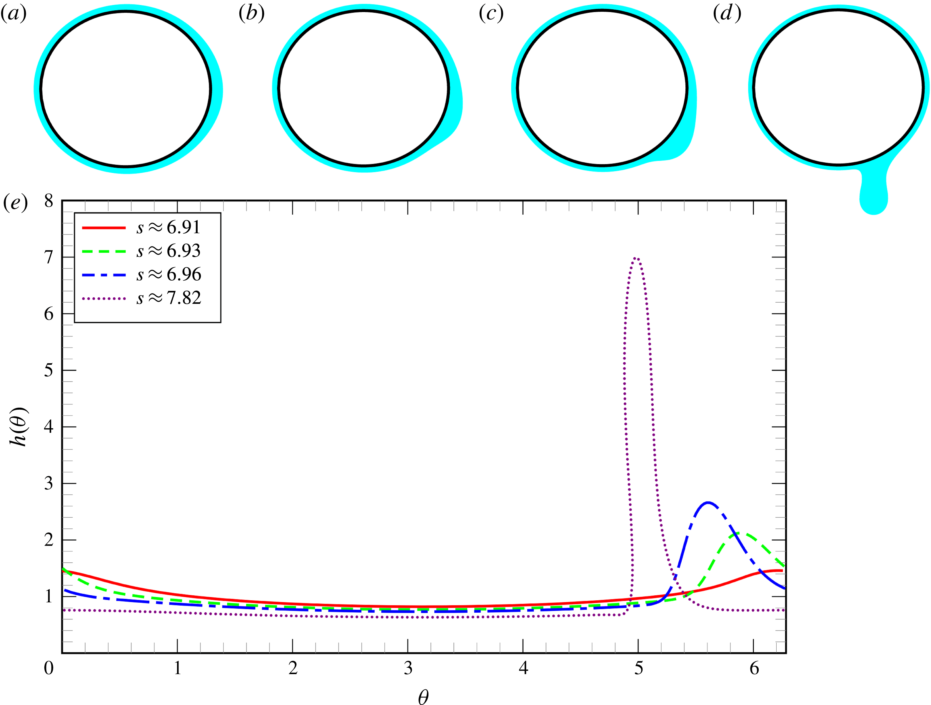
. As the Bond number increases, gravitational forces become more important relative to the capillary forces and a limit point develops for the coating flow, which corresponds to the loss of the static pendant-drop solution. Therefore, this effect is not expected to be captured by the classic lubrication theory. Solutions on the (unstable) upper branch are characterised by the presence of a local neck region, see figure 5(d). This neck becomes thinner as the solution evolves and, consequently, it becomes hard to investigate subsequent limit points that may occur at large rotation numbers. We note that with increasing
 $Bo_{\unicode[STIX]{x1D706}}$
, the limit point moves to larger values of
 $\unicode[STIX]{x1D6FA}_{\unicode[STIX]{x1D706}}$
and that, in addition, further limit points can be observed. For instance, for
 $Bo_{\unicode[STIX]{x1D706}}=200$
, figure 4 shows that within a small range of rotation numbers (
 $1.85\lesssim \unicode[STIX]{x1D6FA}\lesssim 1.92$
) there are at least four steady-state solutions for
 $\unicode[STIX]{x1D706}=0.1$
. Figure 5 shows the four possible solutions and we conjecture that an increasing number of such solutions exist as
 $Bo_{\unicode[STIX]{x1D706}}$
increases. The stability of these steady-state solutions was investigated using time dependent simulations. We concluded that the profiles shown in figure 5(a,c) are stable to small perturbations, whereas the profiles shown in figure 5(a,d) are unstable to small perturbations. Thus, the three limit points are caused by the same eigenvalue crossing the imaginary axis three times. The system is bistable in this region and the final solution reached will depend on the initial conditions. We have not explored the boundaries of the basins of attraction of each solution.
4.2 Rimming flow
Example of rimming-flow profiles obtained from the numerical solution of the Stokes equations for
 $\unicode[STIX]{x1D706}=0.1$
and
 $Bo_{\unicode[STIX]{x1D706}}=200$
for: (a)
 $\unicode[STIX]{x1D6FA}_{\unicode[STIX]{x1D706}}=3$
; (b)
 $\unicode[STIX]{x1D6FA}_{\unicode[STIX]{x1D706}}=1.5$
; (c)
 $\unicode[STIX]{x1D6FA}_{\unicode[STIX]{x1D706}}=1.0$
; (d)
 $\unicode[STIX]{x1D6FA}_{\unicode[STIX]{x1D706}}=0.01$
. The upper panels illustrate the film profiles on the cylinder while the lower panel shows the same profiles as functions
 $h(\unicode[STIX]{x1D703})$
.

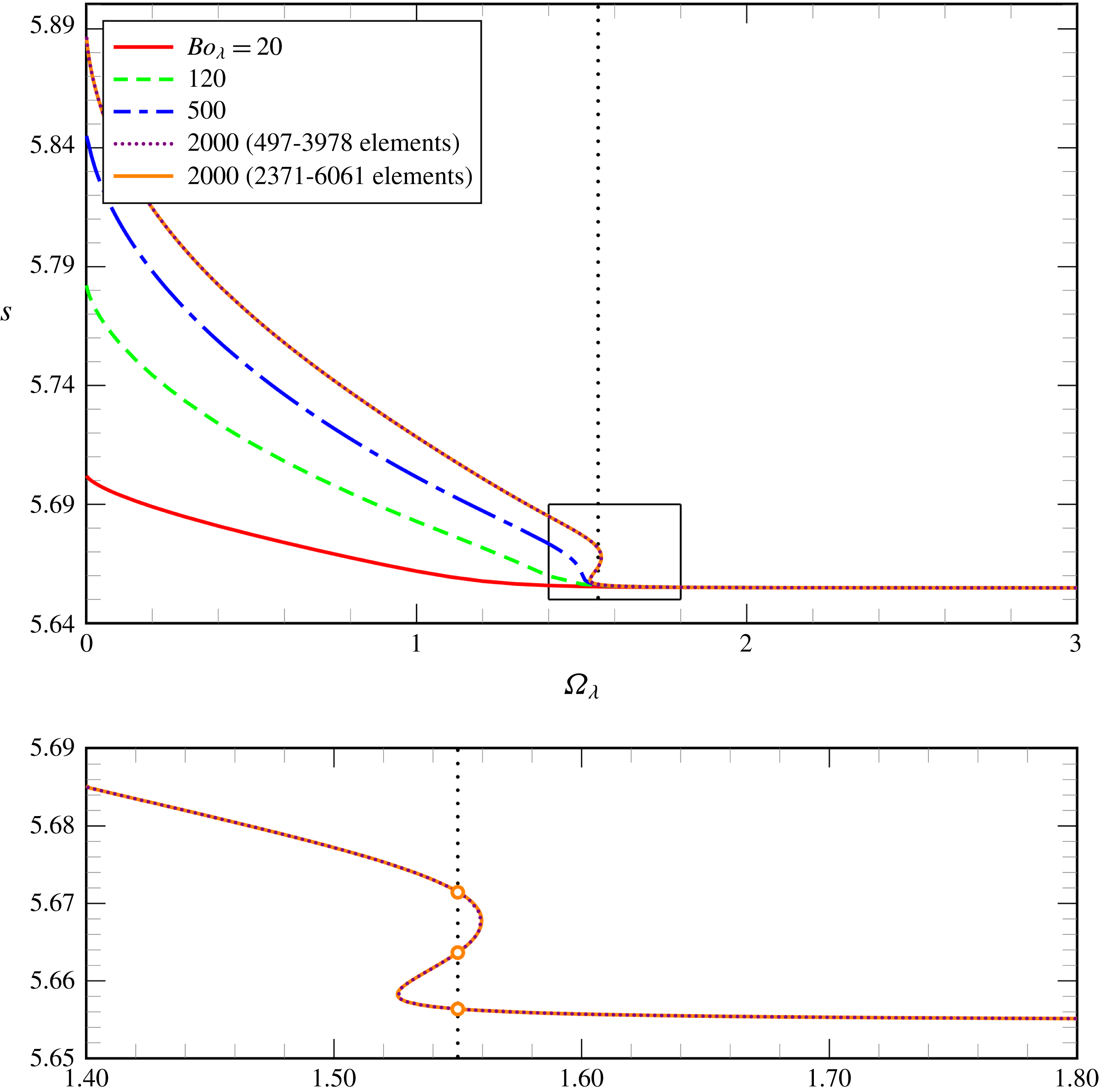
Fluid perimeter
 $s$
for rimming flow as a function of the rotation number
 $\unicode[STIX]{x1D6FA}_{\unicode[STIX]{x1D706}}$
for different Bond numbers
 $Bo_{\unicode[STIX]{x1D706}}$
, as obtained from the numerical solution of the Stokes equations for
 $\unicode[STIX]{x1D706}=0.1$
. The results for
 $Bo_{\unicode[STIX]{x1D706}}=2000$
are presented for two different mesh resolutions, demonstrating agreement to graphical accuracy. The lower panel is an expanded view of the region marked by the box in the upper panel for the case
 $Bo_{\unicode[STIX]{x1D706}}=2000$
only. The multiple solutions at
 $\unicode[STIX]{x1D6FA}_{\unicode[STIX]{x1D706}}=1.55$
(marked by circles on the vertical dotted line) are shown in figure 8.

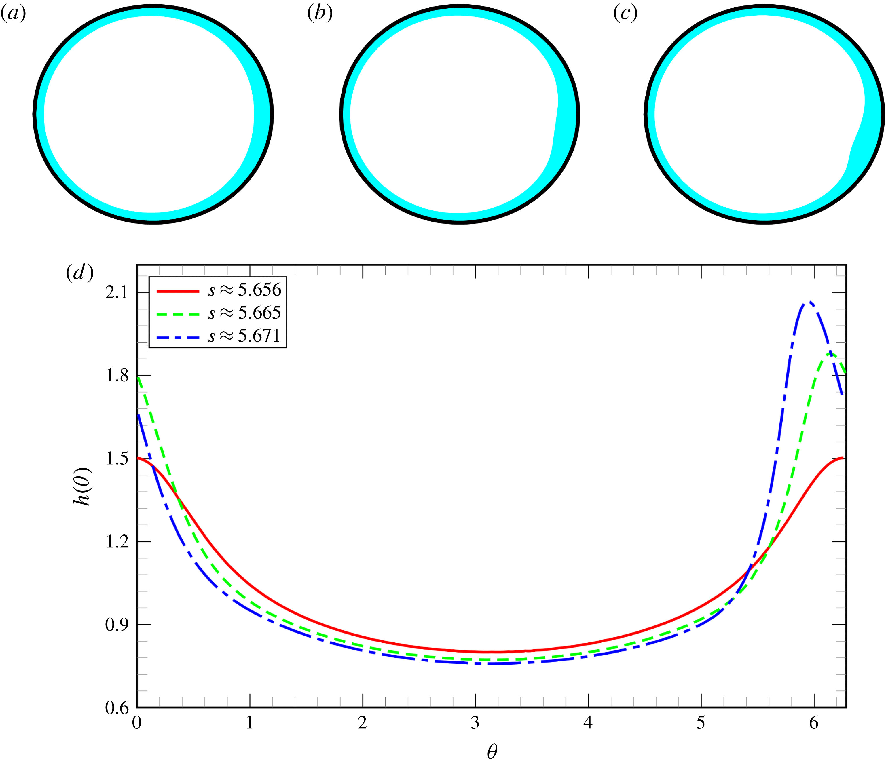
Example of a rimming flow with multiple steady states as obtained from the numerical solution of the Stokes equations for
 $\unicode[STIX]{x1D706}=0.1$
,
 $Bo_{\unicode[STIX]{x1D706}}=2000$
and
 $\unicode[STIX]{x1D6FA}_{\unicode[STIX]{x1D706}}=1.55$
: (a)
 $s\approx 5.656$
; (b)
 $s\approx 5.665$
; (c)
 $s\approx 5.671$
. The upper panels illustrate the film profiles on the cylinder while the lower panel shows the same profiles as functions
 $h(\unicode[STIX]{x1D703})$
.

Figure 6 shows film profiles at different rotation rates for
 $Bo_{\unicode[STIX]{x1D706}}=20$
and is analogous to figure 3. The general evolution is similar in that at high rotation rates the film is approximately uniform and then develops a thicker region near
 $\unicode[STIX]{x1D703}=0$
and a concomitant thinner region near
 $\unicode[STIX]{x1D703}=\unicode[STIX]{x03C0}$
as the rotation rate decreases. As
 $\unicode[STIX]{x1D6FA}_{\unicode[STIX]{x1D706}}\rightarrow 0$
, the film thickness increases and the thickest region moves against the direction of rotation to the base of the cylinder where it forms a puddle, rather than a pendant drop.
Once again we present a global picture of the steady solutions for rimming flow in figure 7, which shows the liquid perimeter s as a function of the rotation number
 $\unicode[STIX]{x1D6FA}_{\unicode[STIX]{x1D706}}$
for different Bond numbers. On comparison to figure 4, one observes significant differences in behaviour between rimming and coating flows. Firstly, figure 7 suggests that for every value of
 $\unicode[STIX]{x1D6FA}_{\unicode[STIX]{x1D706}}$
, we have at least one steady solution, regardless of the value of
 $Bo_{\unicode[STIX]{x1D706}}$
, as argued in the introduction. Secondly, we can see that although multiple solutions do occur for rimming flows, they do so at greater values of the Bond number and only over a limited range of
 $\unicode[STIX]{x1D6FA}_{\unicode[STIX]{x1D706}}$
. Indeed the behaviour in rimming flows is similar to that observed in coating flows at Bond numbers reduced by a factor of approximately 10. This increase in Bond number in rimming flows is in part a consequence of the change in sign of the interface curvature, meaning that, as recognized by Moffatt (Reference Moffatt1977), the surface tension acts as a stabilising force in rimming flow in the sense that a local perturbation that increases (decreases) the fluid height leads to a local increase (decrease) in curvature and hence a local increase (decrease) in fluid pressure, which will drive fluid out of (into) the perturbed region restoring the fluid to its original configuration. In coating flow, however, the altered sign of the curvature means that surface tension is destabilising. The increase in Bond number described above is also due to the fact that for the same rigid cylinder, the magnitude of the curvature (and hence surface-tension-induced normal stress difference) is always greater in rimming flow compared to coating flow. Moreover, gravity also acts to stabilise perturbations in film thickness on the lower half of the cylinder in rimming flow, but will destabilise equivalent perturbations in coating flow. Figure 8 shows the multiple solutions that can occur and although they are superficially similar to the shock-like solutions observed by Benilov et al. (Reference Benilov, Benilov and Kopteva2008) in a lubrication model, these new solutions occur only in the Stokes flow simulations because they feature small scale non-parallel motions that are not captured by the lubrication models, see § 4.3 and § A.1 for further details. We again conducted time dependent numerical investigations to determine the stability of the profiles shown in figure 8. The profiles in figure 8(a,c) are stable to small perturbations, while the profile in figure 8(b) is unstable to small perturbations. Thus, we again have a bistable region albeit over a relatively small region of parameter space. We have also confirmed our simulations are not within the region in which Benilov et al. (Reference Benilov, Lapin and O’Brien2012) claim there are no stable, steady solutions. In § A.2, however, we show that this ‘forbidden’ region does, in fact, contain stable, steady solutions, but that the solutions all have a local region in which the interface overturns and so its position can no longer be represented by a single-valued function of the polar coordinate
 $\unicode[STIX]{x1D703}$
. The numerical method adopted by Benilov et al. (Reference Benilov, Lapin and O’Brien2012) assumed that the interface position was a single-valued function of
 $\unicode[STIX]{x1D703}$
and so could not capture these solutions. We present a more detailed comparison between our results and those of Benilov et al. (Reference Benilov, Benilov and Kopteva2008) and Benilov et al. (Reference Benilov, Lapin and O’Brien2012) in appendix A.
4.3 Lubrication theory versus Stokes
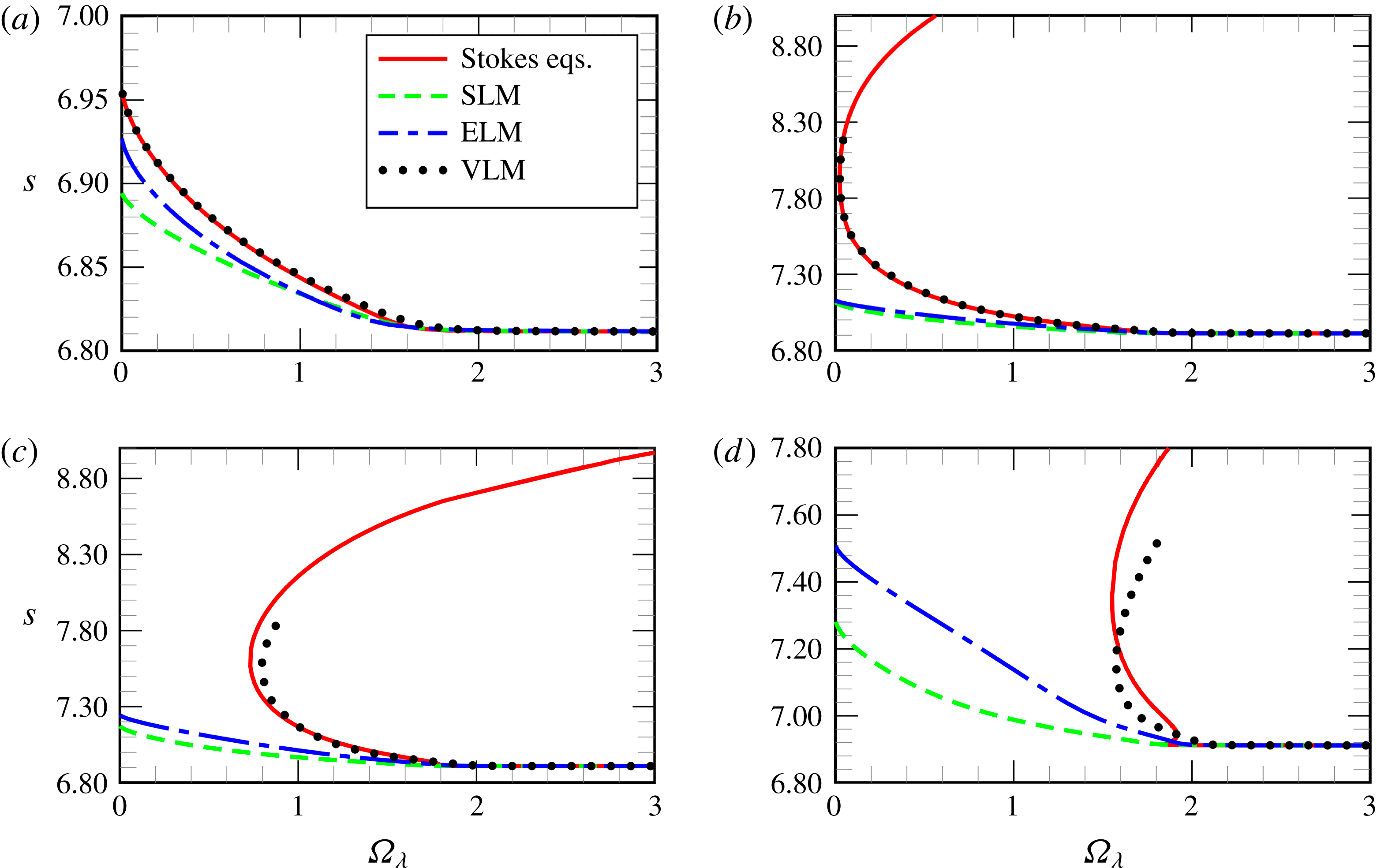
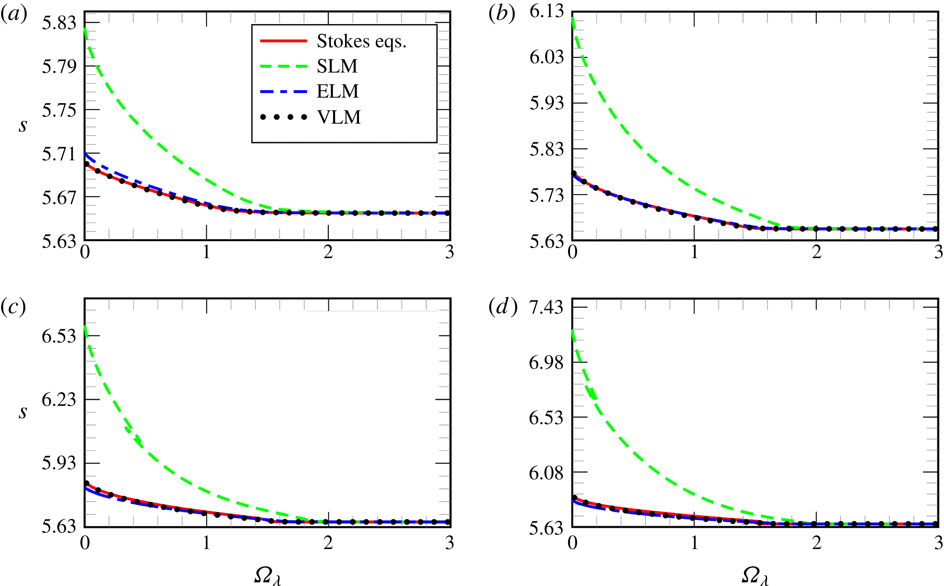
We now examine how well the various lubrication theories presented in § 2.2 reproduce the results of the Stokes flow simulations. Figures 9 and 11 show the same data as in figures 4 and 7 respectively, but with the addition of the results from the three lubrication models. For clarity, the results for the four different values of
 $Bo_{\unicode[STIX]{x1D706}}$
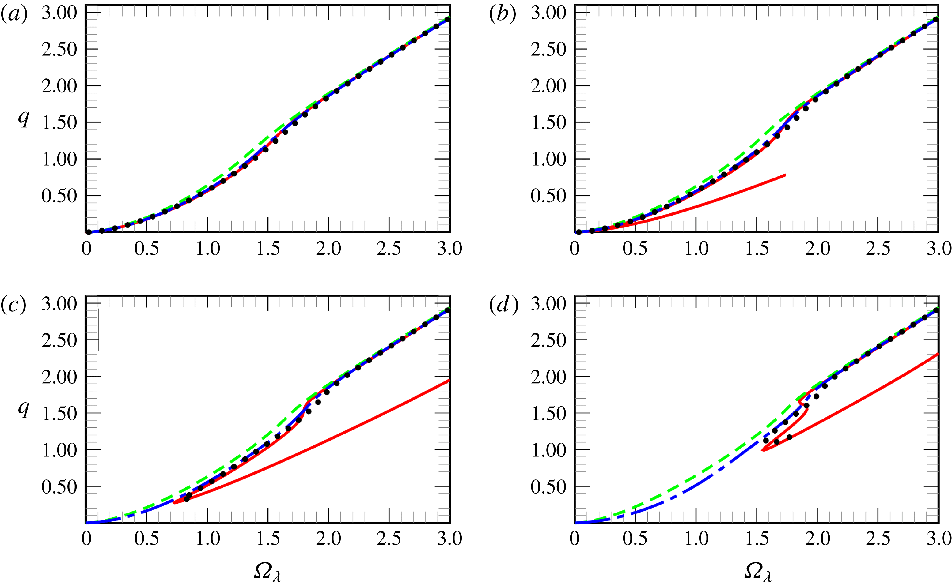
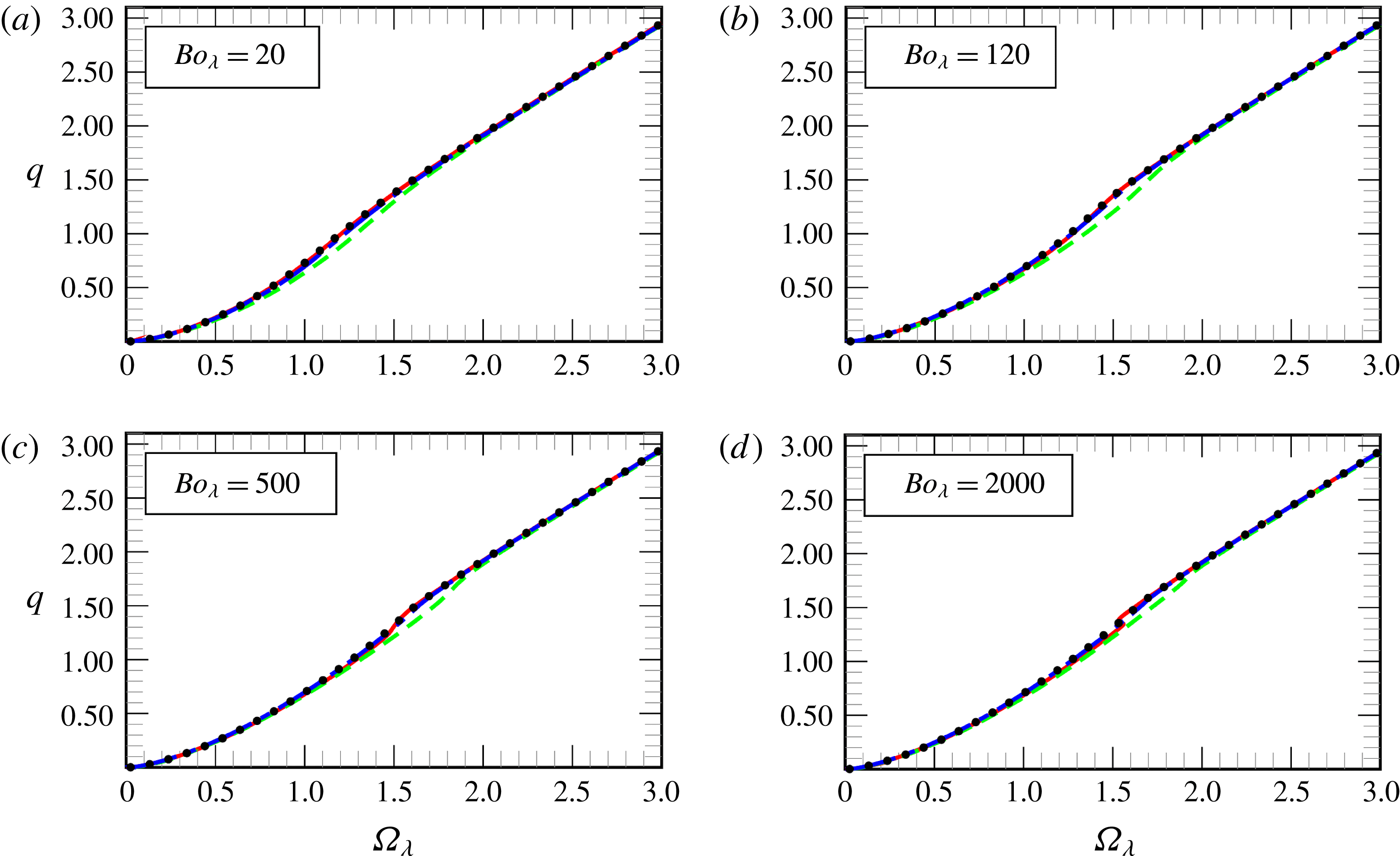
are shown in separate panels. Figures 10 and 12 show the flux
 $q$
as obtained via the Stokes flow simulations and the lubrication models under investigation.
Fluid perimeter
 $s$
for coating flow as a function of the rotation number
 $\unicode[STIX]{x1D6FA}_{\unicode[STIX]{x1D706}}$
for
 $\unicode[STIX]{x1D706}=0.1$
: (a)
 $Bo_{\unicode[STIX]{x1D706}}=20$
; (b)
 $Bo_{\unicode[STIX]{x1D706}}=60$
; (c)
 $Bo_{\unicode[STIX]{x1D706}}=100$
; (d)
 $Bo_{\unicode[STIX]{x1D706}}=200$
. The solid line shows the numerical solution of the Stokes equations; the uniform dashed line shows the numerical solution of the standard lubrication model (SLM); the non-uniform dashed line shows the numerical solution of the extended lubrication model (ELM); the dotted line shows the numerical solution of the variational lubrication model (VLM).

Flux
 $q$
for coating flow as a function of the rotation number
 $\unicode[STIX]{x1D6FA}_{\unicode[STIX]{x1D706}}$
for
 $\unicode[STIX]{x1D706}=0.1$
: (a)
 $Bo_{\unicode[STIX]{x1D706}}=20$
; (b)
 $Bo_{\unicode[STIX]{x1D706}}=60$
; (c)
 $Bo_{\unicode[STIX]{x1D706}}=100$
; (d)
 $Bo_{\unicode[STIX]{x1D706}}=200$
. The graph style is the same as in figure 9.

Fluid perimeter
 $s$
for rimming flow as a function of the rotation number
 $\unicode[STIX]{x1D6FA}_{\unicode[STIX]{x1D706}}$
for
 $\unicode[STIX]{x1D706}=0.1$
: (a)
 $Bo_{\unicode[STIX]{x1D706}}=20$
; (b)
 $Bo_{\unicode[STIX]{x1D706}}=120$
; (c)
 $Bo_{\unicode[STIX]{x1D706}}=500$
; (d)
 $Bo_{\unicode[STIX]{x1D706}}=2000$
. The solid line shows the numerical solution of the Stokes equations; the uniform dashed line shows the numerical solution of the standard lubrication model (SLM); the non-uniform dashed line shows the numerical solution of the extended lubrication model (ELM); the dotted line shows the numerical solution of the variational lubrication model (VLM).

Flux
 $q$
for rimming flow as a function of the rotation number
 $\unicode[STIX]{x1D6FA}_{\unicode[STIX]{x1D706}}$
for
 $\unicode[STIX]{x1D706}=0.1$
: (a)
 $Bo_{\unicode[STIX]{x1D706}}=20$
; (b)
 $Bo_{\unicode[STIX]{x1D706}}=120$
; (c)
 $Bo_{\unicode[STIX]{x1D706}}=500$
; (d)
 $Bo_{\unicode[STIX]{x1D706}}=2000$
. The graph style is the same as in figure 11.

For the coating flow (figures 9 and 10) at high rotation rates
 $\unicode[STIX]{x1D6FA}_{\unicode[STIX]{x1D706}}\gtrsim 2$
all models agree well (to within graphical accuracy), for the Bond number presented. As the rotation rate decreases the SLM and ELM begin to underpredict the true (Stokes flow) perimeter and to overpredict the true flux. As might be expected, the ELM is in closer agreement, but both models are noticeably in error. The underprediction (perimeter) and overprediction (flux) are a consequence of the approximation of the curvature term, which causes the interface to deform less in response to changes in fluid pressure. Importantly, neither SLM nor ELM can capture the limit point that develops when the pendant-drop solution ceases to exist. This is again a consequence of the approximated curvature, which leads to inaccuracies in the hydrostatic balance of the pendant drop at large values of
 $Bo_{\unicode[STIX]{x1D706}}$
. In contrast, the VLM is in good agreement (to graphical accuracy) with the Stokes flow calculations for a much larger range of Bond numbers and can even capture the limit point associated with the loss of the pendant-drop solution. For the highest values of
 $Bo_{\unicode[STIX]{x1D706}}$
, the VLM solutions differ from the Stokes simulations at lower rotation rates. The gross qualitative behaviour is correct, but the multiple solutions near the limit point (cf. lower panel of figure 4) are not reproduced by the VLM suggesting that they involve (small) Stokes regions in which the velocity field differs from the approximate parabolic profile in the lubrication models.
For rimming flow, the ELM and VLM are in reasonable agreement with the Stokes solutions for the majority of cases, which is because the curvature variations as the static puddle solution is approached are relatively small and the linearised curvature approximation remains good. We note, however, that the SLM is always in significant error both quantitatively and qualitatively: the SLM predicts regions of multiple solutions, identified by Benilov et al. (Reference Benilov, Benilov and Kopteva2008), that are not present in the full field equations for our chosen film thickness. Here, we have confirmed by numerical experiment that it is the lack of the hydrostatic pressure term in the SLM that leads to the presence of these multiple solutions because in its absence there is no penalty for changing the interface height. Although the hydrostatic term is a small perturbation relative to the initial film thickness, the multiple solutions in the SLM occur in the region where a sufficiently thick film has formed that the hydrostatic term is significant. We should remark that the presence of a hydrostatic term at leading order in thin-film equations does not preclude the existence of multiple solutions in other flow configurations, e.g. on an inclined plate (Benilov et al. Reference Benilov, Chapman, McLeod, Ockendon and Zubkov2010).
Finally, we summarise our results by identifying regions of validity of each model within the
 $Bo_{\unicode[STIX]{x1D706}}$
–
 $\unicode[STIX]{x1D6FA}_{\unicode[STIX]{x1D706}}$
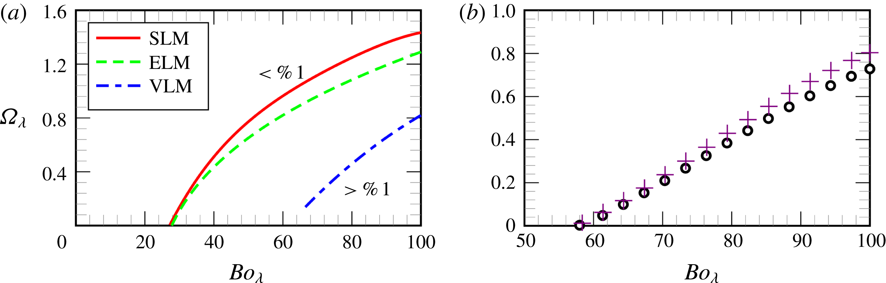
phase space. In figure 13(a), the respective regions above the curves in solid, dashed and dot-dashed lines represent the areas in which the coating perimeter obtained by the SLM, ELM and VLM are within 1 % of the coating perimeter obtained by solving the full Stokes equations for
 $\unicode[STIX]{x1D706}=0.1$
. We can see that in the coating case the SLM and ELM have a very similar performance, but that the VLM is in better agreement with the Stokes equations for a wider range of parameters. Note that if limit points were present only the lower branch of solutions was used in the construction of this Figure. In figure 13(b), the markers represent the location of the limit points in the
 $Bo_{\unicode[STIX]{x1D706}}-\unicode[STIX]{x1D6FA}_{\unicode[STIX]{x1D706}}$
plane for the Stokes equations (black circles) and the VLM (violet crosses). No limit points are found using the SLM or ELM. In the VLM, where the full expression of curvature is maintained, the agreement is not only better but it is also the only considered model that captures the limit point obtained with the full Stokes equations.
Assessment of the regions of validity of the different models for coating flow for
 $\unicode[STIX]{x1D706}=0.1$
. (a) Regions above each curve are those for which the perimeter obtained by each different model is within 1 % of the perimeter obtained from the full Stokes equations: SLM (solid red curve); ELM (dashed green curve); VLM (dot-dashed blue curve). As expected for sufficiently large
 $Bo_{\unicode[STIX]{x1D706}}$
and sufficiently small
 $\unicode[STIX]{x1D6FA}_{\unicode[STIX]{x1D706}}$
, all the lubrication models become inaccurate. (b) Location of the limit point in the Stokes equations (black circles) and VLM (violet crosses). No limit point is predicted in the SLM or ELM.

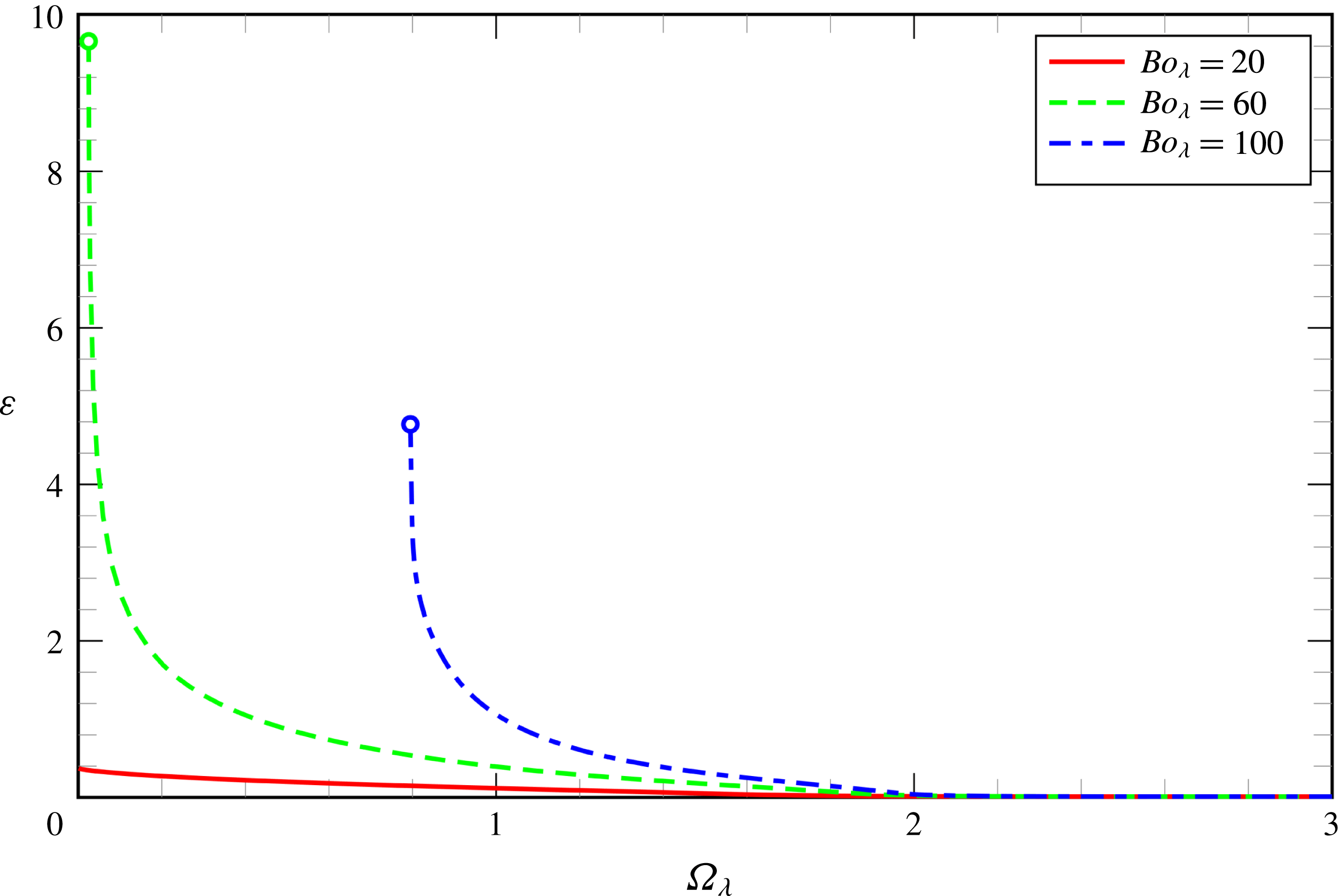
The relative integral error measure
 $\unicode[STIX]{x1D700}$
as a function of the rotation number
 $\unicode[STIX]{x1D6FA}_{\unicode[STIX]{x1D706}}$
for
 $\unicode[STIX]{x1D706}=0.1$
and different Bond numbers
 $Bo_{\unicode[STIX]{x1D706}}$
as obtained via the numerical solution of the VLM. The green and the blue circular dots represent the location of limit point for
 $Bo_{\unicode[STIX]{x1D706}}=60$
and
 $100$
, respectively.

To measure the importance of using the full curvature expression (
 $\unicode[STIX]{x1D705}$
), given in (2.23), rather than its linearised version
 $\unicode[STIX]{x1D705}_{0}=-\unicode[STIX]{x1D6FC}^{-1}+\unicode[STIX]{x2202}_{\unicode[STIX]{x1D703}}^{2}h+h$
in the VLM, we introduce the following relative integral error measure
 $$\begin{eqnarray}\unicode[STIX]{x1D700}=\frac{\sqrt{\displaystyle \int _{0}^{2\unicode[STIX]{x03C0}}(\unicode[STIX]{x1D705}-\unicode[STIX]{x1D705}_{0})^{2}\,\text{d}\unicode[STIX]{x1D703}}}{\sqrt{\displaystyle \int _{0}^{2\unicode[STIX]{x03C0}}\unicode[STIX]{x1D705}^{2}\,\text{d}\unicode[STIX]{x1D703}}}.\end{eqnarray}$$
Figure 14 shows
 $\unicode[STIX]{x1D700}$
as a function of the rotation number
 $(\unicode[STIX]{x1D6FA}_{\unicode[STIX]{x1D706}})$
for
 $\unicode[STIX]{x1D706}=0.1$
and
 $Bo_{\unicode[STIX]{x1D706}}=20$
,
 $60$
and
 $100$
. Clearly for
 $Bo_{\unicode[STIX]{x1D706}}=20$
, we can see that when the surface tension effects are dominant (relatively small Bond number), retaining the full curvature expression does not represent a significant difference neither quantitatively nor qualitatively. For
 $Bo_{\unicode[STIX]{x1D706}}=60$
and
 $100$
, there is an excellent agreement between
 $\unicode[STIX]{x1D705}$
and
 $\unicode[STIX]{x1D705}_{0}$
in the regions where the free surface is essentially a weakly deformed circle. However, when we decrease the rotation rate of the cylinder (decrease
 $\unicode[STIX]{x1D6FA}_{\unicode[STIX]{x1D706}}$
) it becomes evident that the use of
 $\unicode[STIX]{x1D705}_{0}$
causes major changes in the coating profiles. We have verified that when one uses
 $\unicode[STIX]{x1D705}_{0}$
rather than
 $\unicode[STIX]{x1D705}$
in any of our lubrication models, there is always exactly one steady-state solution for every rotation number, but if we use simply
 $\unicode[STIX]{x1D705}$
instead, this is not necessarily true as we can see by the existence of limit points for
 $Bo_{\unicode[STIX]{x1D706}}>60$
.
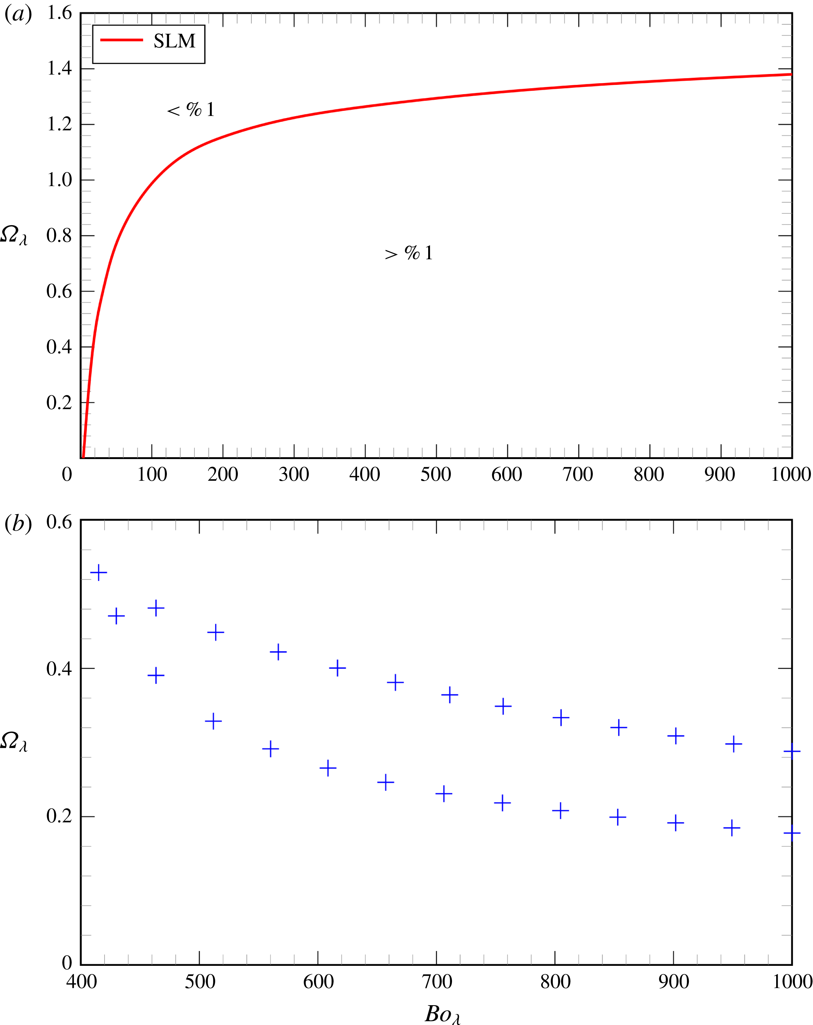
Assessment of the regions of validity of the different models for rimming flow. (a) For the parameter range given the perimeter obtained from the VLM and ELM is always within 1 % of that obtained from the Stokes equations for
 $\unicode[STIX]{x1D706}\leqslant 0.1$
. For the SLM, the perimeter is within 1 % of the Stokes solution above the solid red curve. (b) Location of the limit points in the lubrication models SLM (blue crosses) for
 $\unicode[STIX]{x1D706}=0.1$
. The ELM and VLM do no exhibit limit points when
 $\unicode[STIX]{x1D706}=0.1$
in the parameter regime shown. The Stokes solutions do not exhibit limit points in this regime.

In the case of rimming flow the regions of validity of the models are shown in figure 15(a). We note that for
 $0\leqslant Bo_{\unicode[STIX]{x1D706}}\leqslant 1000$
both perimeters obtained via the ELM and VLM are always within 1 % of the perimeter obtained via the full Stokes equations for
 $\unicode[STIX]{x1D706}=0.1$
. Thus, the region above the solid line represents the area in which the rimming perimeter obtained by the SLM is within 1 % of the rimming perimeter obtained by solving the full Stokes equations for
 $\unicode[STIX]{x1D706}=0.1$
. In figure 15(b), the limit points for the SLM are plotted in the
 $Bo_{\unicode[STIX]{x1D706}}$
–
 $\unicode[STIX]{x1D6FA}_{\unicode[STIX]{x1D706}}$
plane, which means that the area inside the path of limit points represents zones in which there are multiple steady solutions in the SLM. Although this plot is shown for
 $\unicode[STIX]{x1D706}=0.1$
, this region does not depend on the choice of the aspect ratio
 $\unicode[STIX]{x1D706}$
, because the governing equations in the SLM are independent of
 $\unicode[STIX]{x1D706}$
. For
 $\unicode[STIX]{x1D706}=0.1$
, there is no multiple solution zone for
 $0\leqslant Bo_{\unicode[STIX]{x1D706}}\leqslant 1000$
in the ELM, nor in the VLM. Although we do not show the results for different film thicknesses, we have investigated the case
 $\unicode[STIX]{x1D706}=0.05$
when both these models predict the existence of such a zone, auguring for
 $Bo_{\unicode[STIX]{x1D706}}\gtrsim 800$
. Nonetheless, these multiple solutions are not reflected in the full Stokes equations, for which bistability can occur at even higher values of
 $Bo_{\unicode[STIX]{x1D706}}\gtrsim 1000$
. In addition, we also observe that the multiple-solution zones predicted in the ELM and in the VLM for
 $\unicode[STIX]{x1D706}=0.05$
are roughly the same, which means that the inclusion of the full curvature expression in the rimming problem, does not qualitatively affect the solution structure as it does in the coating case.
5 Conclusions
In this paper, we have considered the steady solutions of a film of viscous, incompressible Newtonian fluid on the inside (rimming) or outside (coating) of a cylinder rotating with its axis perpendicular to the direction of gravity. In particular, we have assessed the ranges of validity of lower-dimensional lubrication models and how the qualitative difference between rimming and coating flows can be incorporated into such a model framework. We have used a novel spatially adaptive arclength continuation method combined with finite-element discretisations to solve both the two-dimensional, free-surface Stokes equations and three different lubrication models. Two of the lubrication models have been developed by other authors, but we present a new gradient-dynamics model in which the full expressions of surface and potential energy are taken into account and only the mobility is approximated. This new variational lubrication model is found to exhibit good (less than 1 % relative error in total fluid perimeter) agreement with the Stokes solutions over the widest range of parameters.
We find that using the correct surface energy, i.e. including the exact curvature and the hydrostatic pressure gradient, is required to predict the existence of a limit point that occurs in the coating-flow configuration at low rotation rates. The appearance of the limit point corresponds to the loss of the static pendant-drop solution for sufficiently weak surface tension. In the rimming-flow configuration, no such limit point exists because a static solution, in which fluid accumulates at the base of the cross-section, is always possible. The curvature of the interface for this static solution is relatively small and the behaviour can be well approximated by a linear model, provided that the hydrostatic pressure variation through the thickness of the fluid layer is included. Hence the lubrication models provide more accurate predictions for rimming flow compared to coating-flow configurations with one important exception: the standard (leading-order) lubrication model predicts the existence of multiple solutions, first reported by Benilov et al. (Reference Benilov, Benilov and Kopteva2008) that are not present in the two-dimensional Stokes model for the film thicknesses studied (
 $\unicode[STIX]{x1D706}\geqslant 0.05$
). For the thicker films (
 $\unicode[STIX]{x1D706}=0.1$
), inclusion of the hydrostatic pressure variation through the film thickness is sufficient to suppress these multiple solutions.
Our simulations also demonstrate that the Stokes equations possess previously unobserved multiple, stable and unstable, solutions in both rimming and coating configurations for sufficiently large Bond numbers and intermediate rotation rates. For rimming and coating flows, the system exhibits bistability for these parameters and the final equilibrium state depends on the initial conditions. The alternative solutions feature local regions of increased curvature in which the fluid velocity is relatively low, corresponding to regions in which there is dominant (quasi-static) balance between the hydrostatic pressure gradient and surface tension. This balance would not be expected to occur until the capillary length is sufficiently small, at least comparable to the greatest value of the local film thickness. The average film thickness is comparable to the capillary length when
 $D\sim R/\sqrt{Bo}$
, or
 $Bo_{\unicode[STIX]{x1D706}}\sim \unicode[STIX]{x1D706}^{-3}\approx 1000$
, for our nominal film thickness of
 $\unicode[STIX]{x1D706}=0.1$
. The multiple solutions are seen at lower values of
 $Bo_{\unicode[STIX]{x1D706}}$
in the coating flow configuration because both gravity and surface tension act to increase the local film thickness, compared to the rimming flow where they act to decrease it. These new solutions cannot be found by using any of the simplified lubrication models because they contain regions in which the velocity field is not well approximated by a parallel flow assumption. It is also worth mentioning that the parameter space being examined is realisable experimentally. For example, in the experiment described by Moffatt (Reference Moffatt1977), in which a layer of approximately
 $2.5~\text{mm}$
of golden syrup (diluted with a small amount of water) with
 $\unicode[STIX]{x1D707}=80~\text{g}~\text{cm}^{-1}~\text{s}^{-1}$
at
 $25\,^{\circ }\text{C}$
coated the outside of a Perspex roller of radius
 $R=2.04~\text{cm}$
that rotated about its axis with angular speed
 $\unicode[STIX]{x1D714}$
ranging from
 $21.1~\text{rpm}$
to
 $48.8~\text{rpm}$
, we obtain the following estimates for the dimensionless groups (estimated with
 $\unicode[STIX]{x1D70C}=1~\text{g}~\text{cm}^{-3}$
and
 $\unicode[STIX]{x1D6FE}=50~\text{dyn}~\text{cm}^{-1}$
as in Evans et al. (Reference Evans, Schwartz and Roy2004)):
 $O(\unicode[STIX]{x1D706})\sim 10^{-1}$
,
 $O(Bo_{\unicode[STIX]{x1D706}})\sim 10^{3}$
and
 $O(\unicode[STIX]{x1D6FA}_{\unicode[STIX]{x1D706}})\sim 10$
.
Thus, we conclude that the newly developed variational model is the most appropriate lower-dimensional representation of the system, but it still does not capture the full qualitative behaviour of the Stokes equations. Extensions of these ideas to time-periodic solutions, partially wetting fluids, finite inertia and three-dimensions all for liquid films on a rotating cylinder are the subject of ongoing research. However, it should now also be tested, whether our basic idea of improving lubrication models by bringing them first into gradient-dynamics form and then introducing a more exact form of the underlying energy without changing the mobility function also shows good results in other lubrication-type systems such as those reviewed by Oron, Davis & Bankoff (Reference Oron, Davis and Bankoff1997), Craster & Matar (Reference Craster and Matar2009), Wilczek et al. (Reference Wilczek, Tewes, Gurevich, Köpf, Chi and Thiele2015). For instance, a lubrication model with full curvature was also proposed by Snoeijer (Reference Snoeijer2006) for situations involving moving contact lines (e.g. a contact line advancing down a vertical wall due to gravity) and results in an improvement over the standard lubrication model. The inclusion of modified curvature terms in lubrication models, first suggested by Gauglitz & Radke (Reference Gauglitz and Radke1988), is known to give improved results in a variety of thin-film systems. The gradient-dynamics viewpoint advocated above would suggest that the success of this approximation is due to the better representation of the free energy, which seems to be more important for capturing the qualitative behaviour than correctly resolving the fine details of the flow.
Acknowledgements
A.v.B.L. is supported by the Coordenação de Aperfeiçoamento de Pessoal de Nível Superior (CAPES) under the Grant number 2013/0967-0. We thank the Centre of Nonlinear Science (CeNoS) of the Westfälische Wilhelms Universität at Münster for its support of our collaboration meetings. We would also like to thank Simon Tavener for providing us with a copy of the unpublished work of Benjamin et al. (Reference Benjamin, Pritchard and Tavener1993).
Appendix A. Comparison to earlier work
In this appendix, we shall revisit some of the results obtained in Benilov et al. (Reference Benilov, Benilov and Kopteva2008) and Benilov et al. (Reference Benilov, Lapin and O’Brien2012).
A.1 The paper by Benilov et al. (Reference Benilov, Benilov and Kopteva2008)
In the work by Benilov et al. (Reference Benilov, Benilov and Kopteva2008), the steady flow of a thin liquid film on the inner surface of a rotating cylinder was investigated using the following flux equation:
 $$\begin{eqnarray}q=h-\frac{h^{3}}{3}\cos \unicode[STIX]{x1D703}+\unicode[STIX]{x1D716}\frac{h^{3}}{3}\left(\unicode[STIX]{x2202}_{\unicode[STIX]{x1D703}}^{3}h+\unicode[STIX]{x2202}_{\unicode[STIX]{x1D703}}h\right),\end{eqnarray}$$
where
 $h$
is the film thickness made dimensionless with
 $\unicode[STIX]{x1D6FC}R$
with
 $\unicode[STIX]{x1D6FC}$
given by
 $$\begin{eqnarray}\unicode[STIX]{x1D6FC}=\sqrt{\frac{\unicode[STIX]{x1D707}\unicode[STIX]{x1D714}}{\unicode[STIX]{x1D70C}gR}}.\end{eqnarray}$$
and
 $$\begin{eqnarray}\unicode[STIX]{x1D716}=\frac{\unicode[STIX]{x1D6FE}}{\unicode[STIX]{x1D70C}gR^{2}}\sqrt{\frac{\unicode[STIX]{x1D707}\unicode[STIX]{x1D714}}{\unicode[STIX]{x1D70C}gR}}\end{eqnarray}$$
represents a dimensionless surface tension parameter. The flux equation (A 1) must be solved together with the integral condition
 $$\begin{eqnarray}M=\int _{0}^{2\unicode[STIX]{x03C0}}h\,\text{d}\unicode[STIX]{x1D703},\end{eqnarray}$$
where
 $M$
is a (dimensionless) parameter characterising the net mass of fluid inside the cylinder, and the periodicity condition
 $$\begin{eqnarray}h(\unicode[STIX]{x1D703})=h(\unicode[STIX]{x1D703}+2\unicode[STIX]{x03C0}).\end{eqnarray}$$
Equations (A 1) and (A 4) are, essentially, the SLM equations (2.16) and (2.17) written in a different parametrisation and we note that they also can be derived using standard lubrication theory by assuming that
 $\unicode[STIX]{x1D6FC}\ll 1$
. Using a combination of numerics and asymptotics, Benilov et al. (Reference Benilov, Benilov and Kopteva2008) found that for some small surface tension values, there are certain values of mass
 $M$
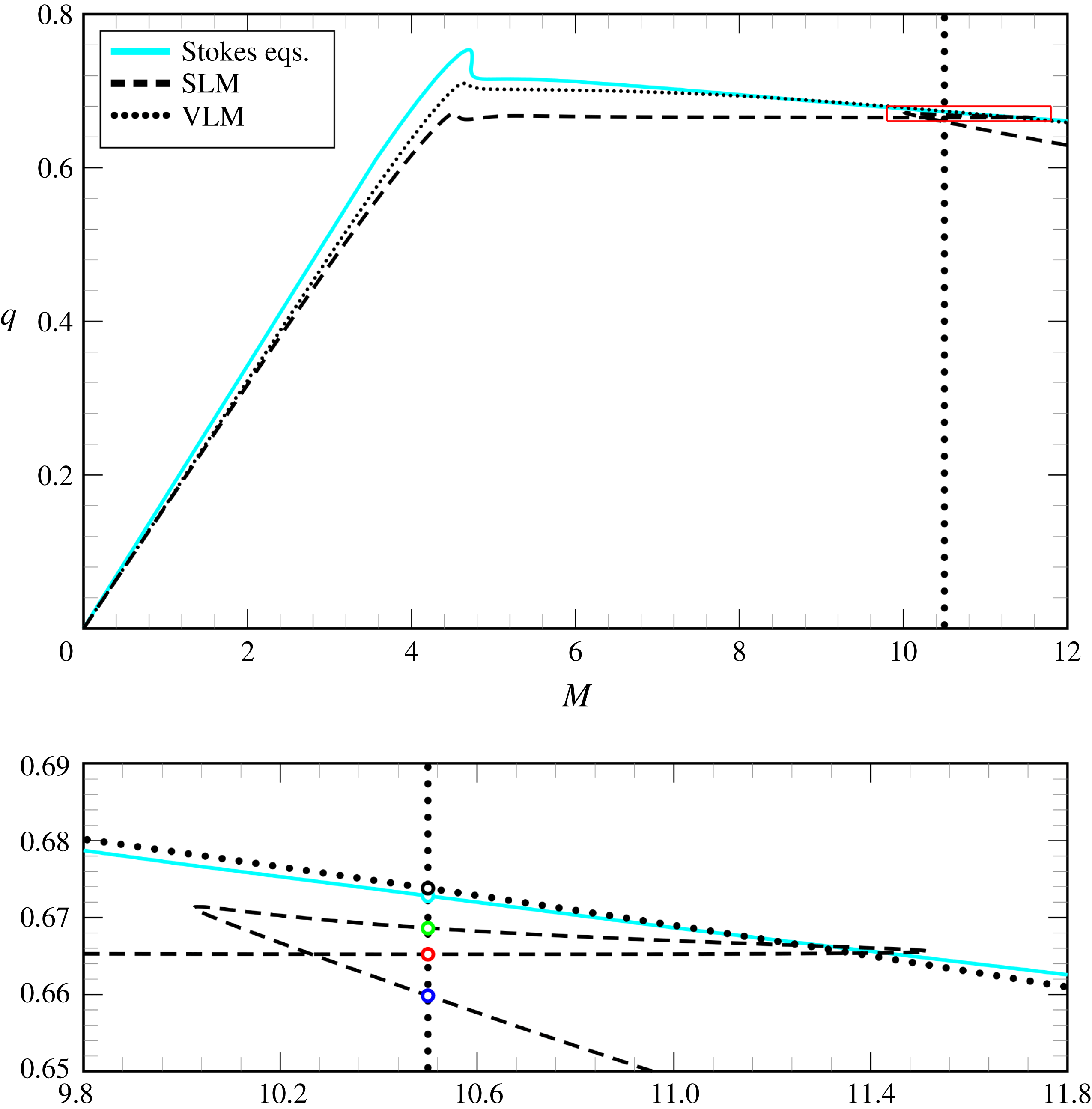
that present up to three steady-state solutions. Figure 16 shows an example of such a situation, as obtained from the numerical solution of (A 1) for
 $\unicode[STIX]{x1D716}=10^{-3}$
. Figure 17 shows the three solutions found at
 $M=10.5$
, each with a different value of
 $q$
. Although the solutions look rather similar, there are clear distinctions in their peak and tail regions.
Flux
 $q$
for rimming flow as a function of the net mass
 $M$
for
 $\unicode[STIX]{x1D716}=10^{-3}$
and
 $\unicode[STIX]{x1D6FC}=0.1$
. The solid line shows the numerical solution of the Stokes equations (A 6) and (A 7); the dashed line shows the numerical solution of the standard lubrication model (SLM), equation (A 1); the dotted line shows the numerical solution of the variational lubrication model (VLM), equation (A 13). The lower panel is an expanded view of the region marked by the box in the upper panel. The solutions at
 $M=10.5$
(marked by circles on the vertical dotted line) are shown in figure 17.

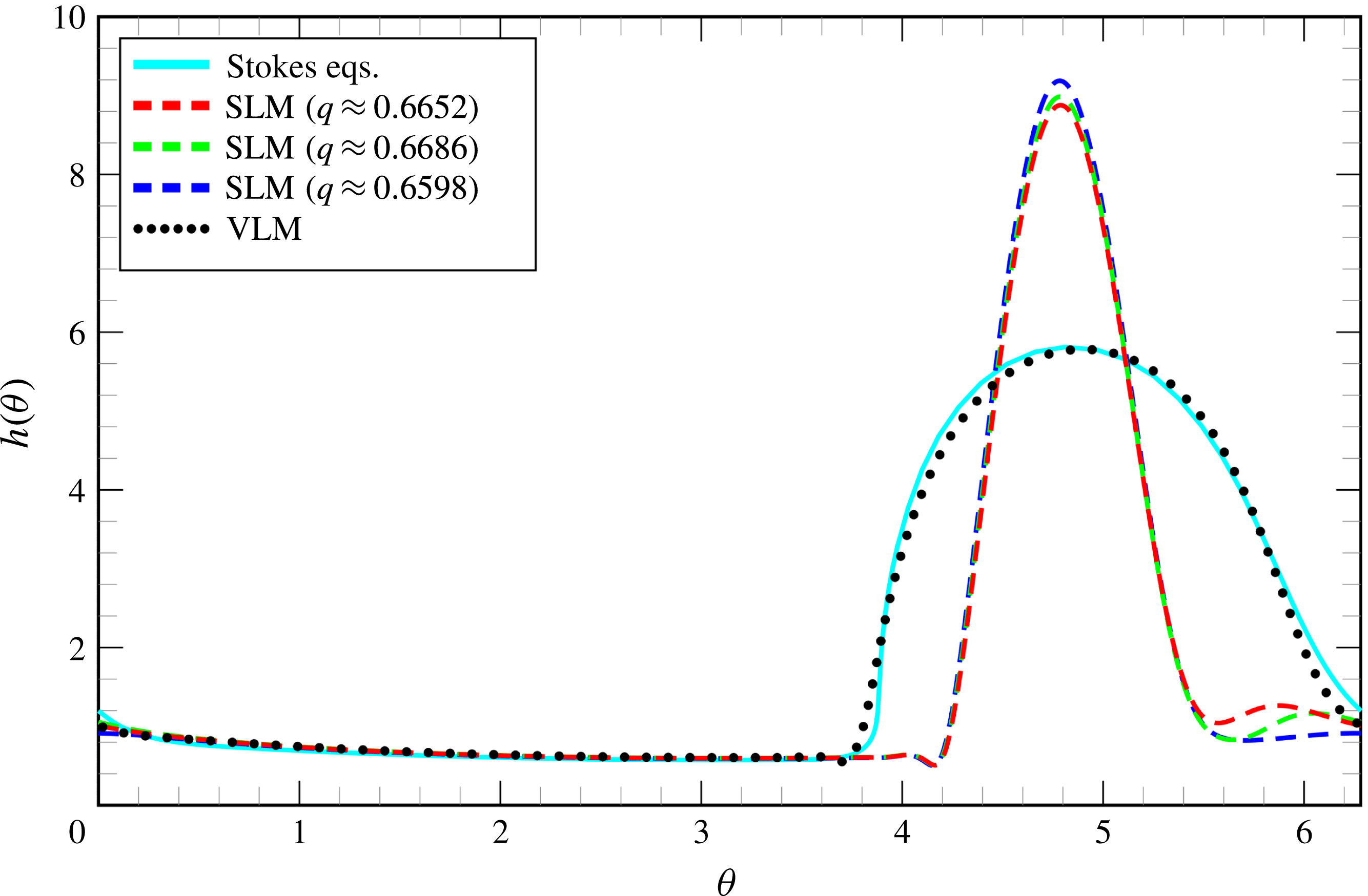
Film profiles
 $h(\unicode[STIX]{x1D703})$
obtained from numerical solution of the Stokes equations (solid line), the standard lubrication model (dashed line) and the variational lubrication model (dashed line) for the rimming-flow problem studied by Benilov et al. (Reference Benilov, Benilov and Kopteva2008) for
 $\unicode[STIX]{x1D6FC}=0.1$
,
 $\unicode[STIX]{x1D716}=0.001$
and
 $M=10.5$
.

We shall revisit this result by solving the two-dimensional steady Stokes equations
 $$\begin{eqnarray}\displaystyle & \displaystyle \unicode[STIX]{x1D735}p=\unicode[STIX]{x1D6FC}^{3}\unicode[STIX]{x1D6FB}^{2}\boldsymbol{u}-\unicode[STIX]{x1D6FC}\boldsymbol{j}, & \displaystyle\end{eqnarray}$$
 $$\begin{eqnarray}\displaystyle & \displaystyle \unicode[STIX]{x1D735}\boldsymbol{\cdot }\boldsymbol{u}=0, & \displaystyle\end{eqnarray}$$
where
 $R$
,
 $\unicode[STIX]{x1D714}R$
and
 $\unicode[STIX]{x1D70C}gR/\unicode[STIX]{x1D6FC}$
were taken as length, velocity and pressure scales, respectively. We require the solutions of the above equations to satisfy the following boundary conditions
 $$\begin{eqnarray}\boldsymbol{u}=\boldsymbol{t}\quad \text{(no-slip condition)}\end{eqnarray}$$
at the surface of the cylinder,
 $$\begin{eqnarray}\displaystyle & \displaystyle \left\{-p\boldsymbol{I}+\frac{1}{\unicode[STIX]{x1D6FC}^{3}}\left[\unicode[STIX]{x1D735}\boldsymbol{u}+(\unicode[STIX]{x1D735}\boldsymbol{u})^{\text{T}}\right]\right\}\boldsymbol{\cdot }\boldsymbol{n}=\unicode[STIX]{x1D716}\unicode[STIX]{x1D705}\boldsymbol{n}\quad \text{(dynamic condition)} & \displaystyle\end{eqnarray}$$
 $$\begin{eqnarray}\displaystyle & \displaystyle \boldsymbol{u}\boldsymbol{\cdot }\boldsymbol{n}=0\quad \text{(kinematic condition)} & \displaystyle\end{eqnarray}$$
at the free surface and we also require that
 $$\begin{eqnarray}\oint \boldsymbol{x}\boldsymbol{\cdot }\boldsymbol{n}\,\text{d}s=\unicode[STIX]{x1D6FC}M\quad \text{(integral condition)},\end{eqnarray}$$
where the line integral is taken along the free-surface boundary. In addition, we also solve the corresponding variational lubrication model (VLM)
 $$\begin{eqnarray}\displaystyle & \displaystyle q=h-\frac{h^{3}}{3}\left[-\unicode[STIX]{x1D716}\unicode[STIX]{x1D705}+(1-\unicode[STIX]{x1D6FC}h)\sin \unicode[STIX]{x1D703}\right], & \displaystyle\end{eqnarray}$$
 $$\begin{eqnarray}\displaystyle & \displaystyle M=\int _{0}^{2\unicode[STIX]{x03C0}}\left(h-\unicode[STIX]{x1D6FC}\frac{h^{2}}{2}\right)\,\text{d}\unicode[STIX]{x1D703}. & \displaystyle\end{eqnarray}$$
A comparison of the fluxes obtained from the numerical solution of the Stokes equations as well as from the SLM and the VLM as a function of the net mass
 $M$
is shown in figure 16 for
 $\unicode[STIX]{x1D6FC}=0.1$
and
 $\unicode[STIX]{x1D716}=10^{-3}$
. The multiple solutions loop found by Benilov et al. (Reference Benilov, Benilov and Kopteva2008) is an artefact of the SLM, because it is neither found in the full model nor in the VLM at these parameter values. Moreover, we note from figure 17 that the film profiles
 $h(\unicode[STIX]{x1D703})$
obtained with the VLM and with the Stokes equations agree really well (shown for
 $M=10.5$
). The solution loop is also absent in the ELM. If one continuously transforms SLM into ELM by means of a homotopy parameter that multiplies the additional terms, one finds that the loop of solutions vanishes in a cusp bifurcation where the limit points merge. We attribute this significant qualitative difference between the solutions obtained from the SLM and those from the ELM, VLM and Stokes equations to the fact that for these solutions a large ‘pool’ of fluid forms. In the ‘pool’ zone the film height peaks and large slopes in the free-surface height can be observed, which means that locally the hydrostatic pressure terms are no longer
 $O(\unicode[STIX]{x1D6FC})$
(a small perturbation), but actually
 $O(1)$
and therefore should be promoted to leading order. As the film thickness reduces the magnitude of the hydrostatic terms will decrease unless the slopes in the ‘pool’ region increase further to compensate. Hence, the multiple solutions found in the SLM would be expected to occur in the Stokes equations for sufficiently thin films. We have found no evidence that multiple solutions occur at these parameter values in the Stokes equations for film thicknesses down to
 $\unicode[STIX]{x1D6FC}=0.05$
, although the distinction between the solutions shown in figure 17 becomes very difficult to detect for such small absolute values of film thickness.
A.2 The paper by Benilov et al. (Reference Benilov, Lapin and O’Brien2012)
This paper examined two distinct regimes of rimming flows on a rotating cylinder: one where surface tension effects are taken into account and one where they are not. In the present work, we shall focus on the former where the authors showed, by solving the Stokes equations numerically, that if a dimensionless capillary coefficient,
 $\unicode[STIX]{x1D6FE}/(\unicode[STIX]{x1D707}\unicode[STIX]{x1D714}R)$
, exceeds a threshold value of 0.23, then a smoothed-shock steady solution always exists. However, the authors claim that if the surface tension is not sufficiently strong (i.e. the capillary coefficient does not exceed the given threshold value) there is a certain ‘forbidden’ region in the parameter space for which the problem does not have stable steady solutions.
In order to verify whether or not the solutions found in the present work are in agreement with the results found in Benilov et al. (Reference Benilov, Lapin and O’Brien2012) it is necessary first to rescale our variables (they chose
 $R$
,
 $\unicode[STIX]{x1D714}R$
,
 $\unicode[STIX]{x1D707}\unicode[STIX]{x1D714}$
and
 $\unicode[STIX]{x1D714}^{-1}$
as length, velocity, pressure and time scales) so that we can interpret our results in terms of the same dimensionless parameters. This can be achieved by introducing the following mappings which transform our dimensionless variables to those used by Benilov et al. (Reference Benilov, Lapin and O’Brien2012):
 $$\begin{eqnarray}\left.\begin{array}{@{}c@{}}\boldsymbol{x}\rightarrow \boldsymbol{x},\quad \boldsymbol{u}\rightarrow \unicode[STIX]{x1D6FA}\boldsymbol{u},\quad p\rightarrow \unicode[STIX]{x1D6FA}p,\quad t\rightarrow \unicode[STIX]{x1D6FA}^{-1}t,\\ \unicode[STIX]{x1D748}\rightarrow \unicode[STIX]{x1D6FA}\unicode[STIX]{x1D748},\quad \unicode[STIX]{x1D705}\rightarrow \unicode[STIX]{x1D705}.\end{array}\right\}\end{eqnarray}$$
In terms of (A 14), the Stokes equations (2.1) take the form
 $$\begin{eqnarray}\displaystyle & \displaystyle \unicode[STIX]{x1D735}p=\unicode[STIX]{x1D6FB}^{2}\boldsymbol{u}-\frac{1}{\unicode[STIX]{x1D6FC}^{2}}\,\boldsymbol{j}, & \displaystyle\end{eqnarray}$$
 $$\begin{eqnarray}\displaystyle & \displaystyle \unicode[STIX]{x1D735}\boldsymbol{\cdot }\boldsymbol{u}=0, & \displaystyle\end{eqnarray}$$
where the dimensionless parameter
 $\unicode[STIX]{x1D6FC}$
is given by
 $$\begin{eqnarray}\unicode[STIX]{x1D6FC}=\sqrt{\unicode[STIX]{x1D6FA}}=\sqrt{\frac{\unicode[STIX]{x1D707}\unicode[STIX]{x1D714}}{\unicode[STIX]{x1D70C}gR}}.\end{eqnarray}$$
The no-slip condition (2.3) now corresponds to
 $$\begin{eqnarray}\boldsymbol{u}=\boldsymbol{t}\end{eqnarray}$$
at the surface of the rotating cylinder. Moreover, the kinematic condition (2.5) retains its original form
 $$\begin{eqnarray}\boldsymbol{u}\boldsymbol{\cdot }\boldsymbol{n}=\unicode[STIX]{x2202}_{t}\boldsymbol{x}\boldsymbol{\cdot }\boldsymbol{n}\end{eqnarray}$$
at the free surface. On the other hand, the dynamic condition (2.6) becomes
 $$\begin{eqnarray}\unicode[STIX]{x1D748}\boldsymbol{\cdot }\boldsymbol{n}=Ca^{-1}\unicode[STIX]{x1D705}\boldsymbol{n},\end{eqnarray}$$
where
 $$\begin{eqnarray}Ca^{-1}=\unicode[STIX]{x1D6FA}^{-1}Bo^{-1}=\frac{\unicode[STIX]{x1D6FE}}{\unicode[STIX]{x1D707}\unicode[STIX]{x1D714}R}\end{eqnarray}$$
is the inverse capillary number (note that
 $Ca^{-1}$
is the aforementioned ‘capillary coefficient’). To introduce the last parameter, it is convenient to note that if we scale the dimensionless film thickness
 $h$
with
 $\unicode[STIX]{x1D6FC}$
, then the mass conservation condition (2.20) requires that
 $$\begin{eqnarray}\int _{0}^{2\unicode[STIX]{x03C0}}\left(h-\unicode[STIX]{x1D6FC}\frac{h^{2}}{2}\right)\,\text{d}\unicode[STIX]{x1D703}=\frac{2\unicode[STIX]{x03C0}}{\unicode[STIX]{x1D6FC}}\left(\unicode[STIX]{x1D706}-\frac{\unicode[STIX]{x1D706}^{2}}{2}\right)\equiv V,\end{eqnarray}$$
where
 $V$
is the volume of liquid within the cylinder. Moreover, it is possible to show (see, e.g. Benjamin et al. (Reference Benjamin, Pritchard and Tavener1993) and O’Brien & Gath (Reference O’Brien and Gath1998)), in the lubrication limit that a shock solution can only exist if
 $$\begin{eqnarray}V_{1}\leqslant V<V_{2},\end{eqnarray}$$
where
 $V_{1}\approx 4.44$
and
 $V_{2}\approx 6.93$
. We note that if
 $V<V_{1}$
Moffatt (Reference Moffatt1977) demonstrated that the film coats the inside of the rotating cylinder in a nearly uniform fashion. On the other hand, if
 $V>V_{2}$
then a pool starts to form at the bottom of the cylinder. For
 $\unicode[STIX]{x1D706}=0.1$
, equations (A 22)–(A 23) give
 $$\begin{eqnarray}0.086\lesssim \unicode[STIX]{x1D6FC}\lesssim 0.134\end{eqnarray}$$
and therefore, on noting that
 $\unicode[STIX]{x1D6FA}=\unicode[STIX]{x1D706}^{2}\unicode[STIX]{x1D6FA}_{\unicode[STIX]{x1D706}}$
, and using (A 17), the relevant range for
 $\unicode[STIX]{x1D6FA}_{\unicode[STIX]{x1D706}}$
is
 $$\begin{eqnarray}0.740\lesssim \unicode[STIX]{x1D6FA}_{\unicode[STIX]{x1D706}}\lesssim 1.796.\end{eqnarray}$$
In the present work, we investigated the following Bond numbers:
-
(i)
 $Bo_{\unicode[STIX]{x1D706}}=20$
,
-
(ii)
$Bo_{\unicode[STIX]{x1D706}}=120$
, -
(iii)
$Bo_{\unicode[STIX]{x1D706}}=500$
, -
(iv)
$Bo_{\unicode[STIX]{x1D706}}=2000$
,


which corresponds, in view of (A 25) and given that
 $Bo_{\unicode[STIX]{x1D706}}=\unicode[STIX]{x1D706}^{-1}Bo$
, to
-
(i)
$27.84\lesssim Ca^{-1}\lesssim 67.57$
, -
(ii)
$4.64\lesssim Ca^{-1}\lesssim 11.26$
, -
(iii)
$1.11\lesssim Ca^{-1}\lesssim 2.70$
, -
(iv)
$0.28\lesssim Ca^{-1}\lesssim 0.68$
.




Note that in all cases,
 $Ca^{-1}$
is larger than 0.23 (the threshold value) and therefore the existence of steady solutions in these intervals is in accordance with the findings in Benilov et al. (Reference Benilov, Lapin and O’Brien2012).
Example of a rimming flow with a shock-like region as obtained from the numerical solution of the Stokes equations for
 $\unicode[STIX]{x1D706}=0.1$
,
 $\unicode[STIX]{x1D6FA}_{\unicode[STIX]{x1D706}}=1$
and
 $Bo_{\unicode[STIX]{x1D706}}=7800$
. The panel (b) is an expanded view of the shock-like region marked by the box in the panel (a).

Furthermore, we decided to investigate the so-called ‘forbidden’ region by solving the Stokes equations for
 $\unicode[STIX]{x1D706}=0.1$
,
 $\unicode[STIX]{x1D6FA}_{\unicode[STIX]{x1D706}}=1$
and
 $Bo_{\unicode[STIX]{x1D706}}=7800$
, which yields
 $Ca^{-1}\approx 0.13$
and
 $\unicode[STIX]{x1D6FC}=0.1$
. As can be seen in figure 18, although
 $Ca^{-1}$
is below the threshold value, a stable shock-like (corner) steady-state solution is found for this set of parameters. We note that the numerical scheme used by Benilov et al. (Reference Benilov, Lapin and O’Brien2012) assumes that the interface position is given by a function
 $h(\unicode[STIX]{x1D703})$
, which cannot represent shock-like regions where
 $h(\unicode[STIX]{x1D703})$
becomes multi-valued. Moreover, Benilov et al. (Reference Benilov, Lapin and O’Brien2012) used a time-dependent solver to approach steady solutions which does not allow unstable solutions to be found. In addition, the restriction on interface shapes prevents computation of stable solutions that are reached via transient regions of interface overturning. We conclude that the results in Benilov et al. (Reference Benilov, Lapin and O’Brien2012) when surface tension is taken into account should be reviewed using a formulation that allows the computation of overturning free surfaces.
Appendix B. Variational approach
This appendix is divided in two parts. In the first part, we briefly introduce Onsager’s variational principle (Onsager Reference Onsager1931a ,Reference Onsager b ), and in the second part we apply it to our problem. Note that a conceptually similar application of Onsager’s variational principle to the modelling of the hydrodynamics of a thin film of a mixture can be found in Xu, Thiele & Qian (Reference Xu, Thiele and Qian2015).
B.1 Onsager’s variational principle
Let
 $a_{1},a_{2},\ldots ,a_{n}$
denote the fluctuations from equilibrium of a set of macroscopic thermodynamic quantities of a closed system, in the following called ‘state variables’. Also, let
 $F=F(a_{1},a_{2},\ldots ,a_{n})$
be the free energy, and let
 $F_{e}=F(0,0,\ldots ,0)$
be its minimum at equilibrium. Then,
 $\unicode[STIX]{x0394}F\equiv F-F_{e}\geqslant 0$
can be expressed as a quadratic form
 $$\begin{eqnarray}\unicode[STIX]{x0394}F=\frac{1}{2}\mathop{\sum }_{i=1}^{n}\mathop{\sum }_{j=1}^{n}\unicode[STIX]{x1D6FD}_{ij}a_{i}a_{j},\end{eqnarray}$$
where
 $\unicode[STIX]{x1D737}$
is a real positive-definite symmetric matrix.
The thermodynamic conjugate to
 $a_{i}$
are the thermodynamic forces defined as
 $$\begin{eqnarray}X_{i}=-\frac{\unicode[STIX]{x2202}\unicode[STIX]{x0394}F}{\unicode[STIX]{x2202}a_{i}}.\end{eqnarray}$$
For small fluctuations, they can be expressed as linear combinations of the state variables, that is
 $$\begin{eqnarray}X_{i}=-\mathop{\sum }_{j=1}^{n}\unicode[STIX]{x1D6FD}_{ij}a_{j}.\end{eqnarray}$$
Assuming that the system is not far from equilibrium, the state variables
 $a_{1},a_{2},\ldots ,a_{n}$
evolve according to the linear relation to the forces
 $$\begin{eqnarray}{\dot{a}}_{i}\equiv \frac{\text{d}}{\text{d}t}a_{i}(t)=\mathop{\sum }_{j=1}^{n}\unicode[STIX]{x1D613}_{ij}X_{j}(t),\end{eqnarray}$$
where the
 $\unicode[STIX]{x1D613}_{ij}$
are called kinetic coefficients. The Onsager principle (Landau & Lifshitz Reference Landau and Lifshitz1980), also known as principle of symmetry of kinetic coefficients, states that
 $\unicode[STIX]{x1D613}_{ij}=L_{ji}$
, that is,
 $\unicode[STIX]{x1D613}$
is a symmetric matrix. Based on this principle, Onsager formulated a variational principle applicable to some irreversible transport processes such as heat conduction, electrical conduction and diffusion.
For isothermal systems, Onsager’s variational principle states that the state evolution equation can be obtained by minimising the so-called Rayleighian (Doi Reference Doi2013)
 $$\begin{eqnarray}{\mathcal{R}}=\mathop{\sum }_{i=1}^{n}\frac{\unicode[STIX]{x2202}F}{\unicode[STIX]{x2202}a_{i}}{\dot{a}}_{i}+\frac{1}{2}\mathop{\sum }_{i=1}^{n}\mathop{\sum }_{j=1}^{n}\unicode[STIX]{x1D701}_{ij}{\dot{a}}_{i}{\dot{a}}_{j}\end{eqnarray}$$
with respect to
 $\dot{a_{1}},\dot{a_{2}},\ldots ,\dot{a_{n}}$
, that is the rates of change of the macroscopic variables
 $a_{1},a_{2},\ldots ,a_{n}$
. The two terms on the right-hand side are physically distinct. The first term is
 ${\dot{F}}\equiv \text{d}F/\text{d}t$
, which is the rate of change of the free energy of the system
 $F=F(a_{1},\ldots ,a_{n})$
. The second term is the energy dissipation function
 $\unicode[STIX]{x1D6F7}$
, which is a quadratic form with the friction coefficient matrix
 $\unicode[STIX]{x1D701}$
forming a positive definite and symmetric matrix.
Minimisation of
 ${\mathcal{R}}$
with respect to the rates
 ${\dot{a}}_{i}$
leads to the kinetic equations
 $$\begin{eqnarray}-\frac{\unicode[STIX]{x2202}F}{\unicode[STIX]{x2202}a_{i}}=\mathop{\sum }_{j=1}^{n}\unicode[STIX]{x1D701}_{ij}{\dot{a}}_{j},\end{eqnarray}$$
which expresses a balance between two forces: the reversible force
 $-\unicode[STIX]{x2202}F/\unicode[STIX]{x2202}a_{i}$
and the friction force
 $\sum _{j=1}^{n}\unicode[STIX]{x1D701}_{ij}{\dot{a}}_{j}$
. Inverting (B 6), one obtains (B 4), i.e.
 $\unicode[STIX]{x1D701}_{ij}^{-1}=\unicode[STIX]{x1D613}_{ij}$
. Also note, that substitution of (B 6) into (B 5) shows that
 $$\begin{eqnarray}{\dot{F}}=-2\unicode[STIX]{x1D6F7}.\end{eqnarray}$$
The Onsager variational principle can be then summarised as follows.
-
(i) Choose appropriate state variables
$a_{1},a_{2},\ldots ,a_{n}$
. -
(ii) Construct the free energy function
$F=F(a_{1},\ldots ,a_{n})$
. -
(iii) Construct the energy dissipation function
$\unicode[STIX]{x1D6F7}$
. -
(iv) Construct the Rayleighian
${\mathcal{R}}={\dot{F}}+\unicode[STIX]{x1D6F7}$
. -
(v) Obtain the time evolution of the state (kinetic equations) by minimising
${\mathcal{R}}$
with respect to the rates
$\dot{a_{i}}$
.




B.2 Application of Onsager’s variational principle to our problem
We note that all the following physical variables and quantities are, unless otherwise stated, dimensional.
The free energy (per unit length) function
 $F=F[h]$
is defined as
 $$\begin{eqnarray}F=\underbrace{\unicode[STIX]{x1D6FE}\oint \text{d}s}_{\mathit{surface}\,\mathit{energy}\,(\mathit{per}\,\mathit{unit}\,\mathit{length})}+\underbrace{\unicode[STIX]{x1D70C}g\iint r\sin \unicode[STIX]{x1D703}\,\text{d}A}_{\mathit{potential}\,\mathit{energy}\,(\mathit{per}\,\mathit{unit}\,\mathit{length})},\end{eqnarray}$$
where the line integral is taken over the fluid perimeter and the area integral is taken over the fluid domain. Alternatively, we can write the previous equation as
 $$\begin{eqnarray}F=\int _{0}^{2\unicode[STIX]{x03C0}}(\unicode[STIX]{x1D6FE}\unicode[STIX]{x1D709}+f)\,\text{d}\unicode[STIX]{x1D703},\end{eqnarray}$$
where
 $\unicode[STIX]{x1D709}\,\text{d}\unicode[STIX]{x1D703}\equiv \sqrt{(R\pm h)^{2}+(\unicode[STIX]{x2202}_{\unicode[STIX]{x1D703}}h)^{2}}\,\text{d}\unicode[STIX]{x1D703}$
corresponds to the line element
 $\text{d}s$
in polar coordinates and
 $f=f(h)$
is given by
 $$\begin{eqnarray}f=\pm \unicode[STIX]{x1D70C}g\int _{R}^{R\pm h}r^{2}\sin \unicode[STIX]{x1D703}\,\text{d}r=\pm \frac{\unicode[STIX]{x1D70C}g}{3}[(R\pm h)^{3}-R^{3}]\sin \unicode[STIX]{x1D703}.\end{eqnarray}$$
The rate of change of
 $F$
is given by
 $$\begin{eqnarray}{\dot{F}}=\int _{0}^{2\unicode[STIX]{x03C0}}\text{d}\unicode[STIX]{x1D703}\unicode[STIX]{x2202}_{t}h\frac{\unicode[STIX]{x1D6FF}F}{\unicode[STIX]{x1D6FF}h}=\int _{0}^{2\unicode[STIX]{x03C0}}\text{d}\unicode[STIX]{x1D703}\unicode[STIX]{x2202}_{t}h\frac{\unicode[STIX]{x1D6FF}}{\unicode[STIX]{x1D6FF}h}\int _{0}^{2\unicode[STIX]{x03C0}}\text{d}\unicode[STIX]{x1D703}^{\prime }(\unicode[STIX]{x1D6FE}\unicode[STIX]{x1D709}+f),\end{eqnarray}$$
and by using the linearity property of the functional derivative, this can be simplified to
 $$\begin{eqnarray}{\dot{F}}=\int _{0}^{2\unicode[STIX]{x03C0}}\text{d}\unicode[STIX]{x1D703}\unicode[STIX]{x2202}_{t}h\frac{\unicode[STIX]{x1D6FF}}{\unicode[STIX]{x1D6FF}h}\left(\unicode[STIX]{x1D6FE}\int _{0}^{2\unicode[STIX]{x03C0}}\text{d}\unicode[STIX]{x1D703}^{\prime }\unicode[STIX]{x1D709}+\int _{0}^{2\unicode[STIX]{x03C0}}\text{d}\unicode[STIX]{x1D703}^{\prime }f\right).\end{eqnarray}$$
We note that
 $$\begin{eqnarray}\displaystyle \frac{\unicode[STIX]{x1D6FF}}{\unicode[STIX]{x1D6FF}h}\int _{0}^{2\unicode[STIX]{x03C0}}\text{d}\unicode[STIX]{x1D703}^{\prime }\unicode[STIX]{x1D709} & = & \displaystyle \frac{\unicode[STIX]{x1D6FF}}{\unicode[STIX]{x1D6FF}h}\int _{0}^{2\unicode[STIX]{x03C0}}\text{d}\unicode[STIX]{x1D703}^{\prime }\left[\sqrt{(R\pm h)^{2}+\left(\unicode[STIX]{x2202}_{\unicode[STIX]{x1D703}}h\right)^{2}}\right]\nonumber\\ \displaystyle & = & \displaystyle \pm \frac{(R\pm h)}{\sqrt{(R\pm h)^{2}+(\unicode[STIX]{x2202}_{\unicode[STIX]{x1D703}}h)^{2}}}-\unicode[STIX]{x2202}_{\unicode[STIX]{x1D703}}\left[\frac{\unicode[STIX]{x2202}_{\unicode[STIX]{x1D703}}h}{\sqrt{(R\pm h)^{2}+(\unicode[STIX]{x2202}_{\unicode[STIX]{x1D703}}h)^{2}}}\right]\nonumber\\ \displaystyle & = & \displaystyle \frac{\pm (R\pm h)-\unicode[STIX]{x2202}_{\unicode[STIX]{x1D703}}^{2}h}{\sqrt{(R\pm h)^{2}+(\unicode[STIX]{x2202}_{\unicode[STIX]{x1D703}}h)^{2}}}+\frac{(\unicode[STIX]{x2202}_{\unicode[STIX]{x1D703}}h)^{2}\left[\pm (R\pm h)+\unicode[STIX]{x2202}_{\unicode[STIX]{x1D703}}^{2}h\right]}{\left[(R\pm h)^{2}+\left(\unicode[STIX]{x2202}_{\unicode[STIX]{x1D703}}h\right)^{2}\right]^{3/2}}\nonumber\\ \displaystyle & = & \displaystyle (R\pm h)\left\{\frac{\pm (R\pm h)^{2}\pm 2(\unicode[STIX]{x2202}_{\unicode[STIX]{x1D703}}h)^{2}-(R\pm h)\unicode[STIX]{x2202}_{\unicode[STIX]{x1D703}}^{2}h}{\left[(R\pm h)^{2}+(\unicode[STIX]{x2202}_{\unicode[STIX]{x1D703}}h)^{2}\right]^{3/2}}\right\}\nonumber\\ \displaystyle & = & \displaystyle -(R\pm h)\unicode[STIX]{x1D705},\end{eqnarray}$$
where the last equality follows from (2.23), and that
 $$\begin{eqnarray}\frac{\unicode[STIX]{x1D6FF}}{\unicode[STIX]{x1D6FF}h}\int _{0}^{2\unicode[STIX]{x03C0}}\text{d}\unicode[STIX]{x1D703}^{\prime }f={\displaystyle \frac{\text{d}f}{\text{d}h}}=\unicode[STIX]{x1D70C}g(R\pm h)^{2}\sin (\unicode[STIX]{x1D703}).\end{eqnarray}$$
The variation of the free energy with respect to the rate
 $\unicode[STIX]{x2202}_{t}h$
is then given by
 $$\begin{eqnarray}\unicode[STIX]{x1D6FF}{\dot{F}}=\int _{0}^{2\unicode[STIX]{x03C0}}[-\unicode[STIX]{x1D6FE}(R\pm h)\unicode[STIX]{x1D705}+f^{\prime }]\unicode[STIX]{x1D6FF}(\unicode[STIX]{x2202}_{t}h)\,\text{d}\unicode[STIX]{x1D703},\end{eqnarray}$$
where
 $f^{\prime }=f^{\prime }(h)=\text{d}f/\text{d}h$
. The (viscous) dissipation function
 $\unicode[STIX]{x1D6F7}$
, which is the rate at which (mechanical) work is converted into internal thermal energy, is given by
 $$\begin{eqnarray}\unicode[STIX]{x1D6F7}=\frac{1}{2}\iint \left(\boldsymbol{T}\boldsymbol{ : }\unicode[STIX]{x1D735}\boldsymbol{u}\right)\,\text{d}A.\end{eqnarray}$$
Note that, in polar coordinates, the double dot product
 $\boldsymbol{T}\boldsymbol{ : }\unicode[STIX]{x1D735}\boldsymbol{u}$
for an incompressible Newtonian liquid can be written as (Bird, Stewart & Lightfoot Reference Bird, Stewart and Lightfoot2002):
 $$\begin{eqnarray}\boldsymbol{T}\boldsymbol{ : }\unicode[STIX]{x1D735}\boldsymbol{u}=2\unicode[STIX]{x1D707}\left[(\unicode[STIX]{x2202}_{r}u)^{2}+\left(\frac{\unicode[STIX]{x2202}_{\unicode[STIX]{x1D703}}v}{r}+\frac{v}{r}\right)^{2}\right]+\unicode[STIX]{x1D707}\left[\unicode[STIX]{x2202}_{r}v-\frac{v}{r}+\frac{\unicode[STIX]{x2202}_{\unicode[STIX]{x1D703}}u}{r}\right]^{2}.\end{eqnarray}$$
In the thin-film limit,
 $\boldsymbol{T}\boldsymbol{ : }\unicode[STIX]{x1D735}\boldsymbol{u}$
is represented simply by
 $\unicode[STIX]{x1D707}(\unicode[STIX]{x2202}_{r}v)^{2}$
and, consequently,
 $$\begin{eqnarray}\unicode[STIX]{x1D6F7}=\frac{\unicode[STIX]{x1D707}}{2}\iint (\unicode[STIX]{x2202}_{r}v)^{2}\,\text{d}A.\end{eqnarray}$$
The variation of
 $\unicode[STIX]{x1D6F7}$
with respect to
 $v$
is then given from the definition of variational derivative,
 $$\begin{eqnarray}\displaystyle \unicode[STIX]{x1D6FF}\unicode[STIX]{x1D6F7} & = & \displaystyle {\displaystyle \frac{\unicode[STIX]{x1D707}}{2}}\iint \lim _{\unicode[STIX]{x1D716}\rightarrow 0}\left\{{\displaystyle \frac{\left[\unicode[STIX]{x2202}_{r}(v+\unicode[STIX]{x1D716}\unicode[STIX]{x1D6FF}v)\right]^{2}-(\unicode[STIX]{x2202}_{r}v)^{2}}{\unicode[STIX]{x1D716}}}\right\}\,\text{d}A\nonumber\\ \displaystyle & = & \displaystyle {\displaystyle \frac{\unicode[STIX]{x1D707}}{2}}\iint \lim _{\unicode[STIX]{x1D716}\rightarrow 0}\left\{2\unicode[STIX]{x2202}_{r}v\unicode[STIX]{x2202}_{r}(\unicode[STIX]{x1D6FF}v)+\unicode[STIX]{x1D716}\left[\unicode[STIX]{x2202}_{r}(\unicode[STIX]{x1D6FF}v)\right]^{2}\right\}\,\text{d}A\nonumber\\ \displaystyle & = & \displaystyle \unicode[STIX]{x1D707}\iint \unicode[STIX]{x2202}_{r}v\unicode[STIX]{x2202}_{r}\left(\unicode[STIX]{x1D6FF}v\right)\,\text{d}A\nonumber\\ \displaystyle & = & \displaystyle \pm \unicode[STIX]{x1D707}\int _{0}^{2\unicode[STIX]{x03C0}}\int _{R}^{R\pm h}(r\unicode[STIX]{x2202}_{r}v)\unicode[STIX]{x2202}_{r}(\unicode[STIX]{x1D6FF}v)\,\text{d}r\,\text{d}\unicode[STIX]{x1D703}.\end{eqnarray}$$
A single integration by parts in the previous integral yields
 $$\begin{eqnarray}\displaystyle \unicode[STIX]{x1D6FF}\unicode[STIX]{x1D6F7} & = & \displaystyle \left.\mp \unicode[STIX]{x1D707}\int _{0}^{2\unicode[STIX]{x03C0}}\int _{R}^{R\pm h}\unicode[STIX]{x2202}_{r}(r\unicode[STIX]{x2202}_{r}v)\unicode[STIX]{x1D6FF}v\,\text{d}r\,\text{d}\unicode[STIX]{x1D703}\pm \unicode[STIX]{x1D707}\int _{0}^{2\unicode[STIX]{x03C0}}r\unicode[STIX]{x2202}_{r}v\unicode[STIX]{x1D6FF}v\right|_{r=R}^{r=R\pm h}\,\text{d}\unicode[STIX]{x1D703}\nonumber\\ \displaystyle & = & \displaystyle \left.\mp \unicode[STIX]{x1D707}\int _{0}^{2\unicode[STIX]{x03C0}}\int _{R}^{R\pm h}r\left(\unicode[STIX]{x2202}_{r}^{2}v+\frac{\unicode[STIX]{x2202}_{r}v}{r}\right)\unicode[STIX]{x1D6FF}v\,\text{d}r\,\text{d}\unicode[STIX]{x1D703}\pm \unicode[STIX]{x1D707}\int _{0}^{2\unicode[STIX]{x03C0}}r\unicode[STIX]{x2202}_{r}v\unicode[STIX]{x1D6FF}v\right|_{r=R}^{r=R\pm h}\,\text{d}\unicode[STIX]{x1D703}.\end{eqnarray}$$
In the thin-film limit, the previous equation reduces to
 $$\begin{eqnarray}\left.\unicode[STIX]{x1D6FF}\unicode[STIX]{x1D6F7}=\mp \unicode[STIX]{x1D707}R\int _{0}^{2\unicode[STIX]{x03C0}}\int _{R}^{R\pm h}\unicode[STIX]{x2202}_{r}^{2}v\unicode[STIX]{x1D6FF}v\,\text{d}r\,\text{d}\unicode[STIX]{x1D703}\pm \unicode[STIX]{x1D707}\int _{0}^{2\unicode[STIX]{x03C0}}r\unicode[STIX]{x2202}_{r}v\unicode[STIX]{x1D6FF}v\right|_{r=R}^{r=R\pm h}\,\text{d}\unicode[STIX]{x1D703}.\end{eqnarray}$$
Next, we use the pressure
 $p(r,\unicode[STIX]{x1D703})$
as a Lagrange multiplier to impose the incompressibility constraint,
 $\unicode[STIX]{x1D735}\boldsymbol{\cdot }\boldsymbol{u}=0$
, by adding the following term
 $C$
to the Rayleighian
 ${\mathcal{R}}$
:
 $$\begin{eqnarray}C=\iint [-p(\unicode[STIX]{x1D735}\boldsymbol{\cdot }\boldsymbol{u})]\,\text{d}A,\end{eqnarray}$$
which can be integrated by parts using the well-known Gauss’s divergence theorem to give
 $$\begin{eqnarray}C=\iint \unicode[STIX]{x1D735}p\boldsymbol{\cdot }\boldsymbol{u}\,\text{d}A-\oint pv_{n}\,\text{d}s\end{eqnarray}$$
 $$\begin{eqnarray}=\pm \int _{0}^{2\unicode[STIX]{x03C0}}\int _{R}^{R\pm h}\left(u\unicode[STIX]{x2202}_{r}p+\frac{v}{r}\unicode[STIX]{x2202}_{\unicode[STIX]{x1D703}}p\right)r\,\text{d}r\,\text{d}\unicode[STIX]{x1D703}\mp \int _{0}^{2\unicode[STIX]{x03C0}}pv_{n}\unicode[STIX]{x1D709}\,\text{d}\unicode[STIX]{x1D703},\end{eqnarray}$$
where
 $v_{n}=\boldsymbol{u}\boldsymbol{\cdot }\boldsymbol{n}$
is the outward normal velocity at the free surface. The variation of
 $C$
with respect to the rates
 $u$
and
 $v$
is then found to be
 $$\begin{eqnarray}\unicode[STIX]{x1D6FF}C=\pm \int _{0}^{2\unicode[STIX]{x03C0}}\int _{R}^{R\pm h}\left(\unicode[STIX]{x1D6FF}u\unicode[STIX]{x2202}_{r}p+\frac{\unicode[STIX]{x1D6FF}v}{r}\unicode[STIX]{x2202}_{\unicode[STIX]{x1D703}}p\right)r\,\text{d}r\,\text{d}\unicode[STIX]{x1D703}\mp \int _{0}^{2\unicode[STIX]{x03C0}}p\unicode[STIX]{x1D6FF}v_{n}\unicode[STIX]{x1D709}\,\text{d}\unicode[STIX]{x1D703}.\end{eqnarray}$$
Using the kinematic condition
 $$\begin{eqnarray}v_{n}=(R\pm h)\unicode[STIX]{x1D709}^{-1}\unicode[STIX]{x2202}_{t}h\quad \text{at}~r=R\pm h,\end{eqnarray}$$
we can write
 $\unicode[STIX]{x1D6FF}C$
as
 $$\begin{eqnarray}\unicode[STIX]{x1D6FF}C=\pm \int _{0}^{2\unicode[STIX]{x03C0}}\int _{R}^{R\pm h}\left(\unicode[STIX]{x1D6FF}u\unicode[STIX]{x2202}_{r}p+\frac{\unicode[STIX]{x1D6FF}v}{r}\unicode[STIX]{x2202}_{\unicode[STIX]{x1D703}}p\right)r\,\text{d}r\,\text{d}\unicode[STIX]{x1D703}\mp \int _{0}^{2\unicode[STIX]{x03C0}}p(R\pm h)\unicode[STIX]{x1D6FF}\left(\unicode[STIX]{x2202}_{t}h\right)\,\text{d}\unicode[STIX]{x1D703}.\end{eqnarray}$$
Hence, from the expressions obtained above we can write
 $\unicode[STIX]{x1D6FF}{\mathcal{R}}=\unicode[STIX]{x1D6FF}{\dot{F}}+\unicode[STIX]{x1D6FF}\unicode[STIX]{x1D6F7}+\unicode[STIX]{x1D6FF}C$
as a linear combination of
 $\unicode[STIX]{x1D6FF}u$
,
 $\unicode[STIX]{x1D6FF}v$
and
 $\unicode[STIX]{x1D6FF}(\unicode[STIX]{x2202}_{t}h)$
. Minimising
 ${\mathcal{R}}$
with respect to
 $\unicode[STIX]{x2202}_{t}h$
gives the pressure at the free surface:
 $$\begin{eqnarray}p=\mp \unicode[STIX]{x1D6FE}\unicode[STIX]{x1D705}+\unicode[STIX]{x1D70C}g(R\pm h)\sin \unicode[STIX]{x1D703}\quad \text{at}~r=R\pm h.\end{eqnarray}$$
Minimising
 ${\mathcal{R}}$
with respect to
 $u$
gives
 $$\begin{eqnarray}\unicode[STIX]{x2202}_{r}p=0,\end{eqnarray}$$
i.e. the pressure varies uniformly in the radial direction. Minimising
 ${\mathcal{R}}$
with respect to
 $v$
leads to
 $$\begin{eqnarray}\unicode[STIX]{x2202}_{\unicode[STIX]{x1D703}}p-\unicode[STIX]{x1D707}R\unicode[STIX]{x2202}_{r}^{2}v=0.\end{eqnarray}$$
Lastly, minimising
 ${\mathcal{R}}$
with respect to
 $v$
evaluated at the free surface gives
 $$\begin{eqnarray}\unicode[STIX]{x2202}_{r}v=0\quad \text{at}~r=R\pm h,\end{eqnarray}$$
which is the tangential stress boundary condition at the free surface. In the dimensionless scaled form (see § 2), the governing equations are given by
 $$\begin{eqnarray}\displaystyle & \displaystyle \unicode[STIX]{x2202}_{\unicode[STIX]{x1D702}}p=0, & \displaystyle\end{eqnarray}$$
 $$\begin{eqnarray}\displaystyle & \displaystyle \unicode[STIX]{x2202}_{\unicode[STIX]{x1D703}}p-\unicode[STIX]{x2202}_{\unicode[STIX]{x1D702}}^{2}v=0, & \displaystyle\end{eqnarray}$$
where the asterisks have been omitted, and they are to be solved together with the boundary conditions
 $$\begin{eqnarray}\displaystyle & \displaystyle p=-Bo_{\unicode[STIX]{x1D706}}^{-1}\unicode[STIX]{x1D705}+(1+\unicode[STIX]{x1D6FC}h)\sin \unicode[STIX]{x1D703}\quad \text{at}~\unicode[STIX]{x1D702}=h, & \displaystyle\end{eqnarray}$$
 $$\begin{eqnarray}\displaystyle & \displaystyle v=\unicode[STIX]{x1D6FA}_{\unicode[STIX]{x1D706}}\quad \text{at}~\unicode[STIX]{x1D702}=0, & \displaystyle\end{eqnarray}$$
 $$\begin{eqnarray}\displaystyle & \displaystyle \unicode[STIX]{x2202}_{\unicode[STIX]{x1D702}}v=0\quad \text{at}~\unicode[STIX]{x1D702}=h. & \displaystyle\end{eqnarray}$$
Solving (B 32) subject to the boundary condition (B 34), we obtain the following expression for the fluid pressure
 $$\begin{eqnarray}p=-Bo_{\unicode[STIX]{x1D706}}^{-1}\unicode[STIX]{x1D705}+(1+\unicode[STIX]{x1D6FC}h)\sin \unicode[STIX]{x1D703},\end{eqnarray}$$
which contains the contributions of both Laplace pressure
 $-Bo^{-1}\unicode[STIX]{x1D705}$
and hydrostatic pressures
 $(1+\unicode[STIX]{x1D6FC}h)\sin \unicode[STIX]{x1D703}$
. Substituting it in (B 33), and applying the boundary conditions (B 35) and (B 36), we find that
 $$\begin{eqnarray}v=\unicode[STIX]{x1D6FA}_{\unicode[STIX]{x1D706}}+\left(\frac{\unicode[STIX]{x1D702}^{2}}{2}-\unicode[STIX]{x1D702}h\right)\unicode[STIX]{x2202}_{\unicode[STIX]{x1D703}}[-Bo^{-1}\unicode[STIX]{x1D705}+(1+\unicode[STIX]{x1D6FC}h)\sin \unicode[STIX]{x1D703}].\end{eqnarray}$$
Hence, the expression for the dimensionless flux
 $q=\int _{0}^{h}v\,\text{d}\unicode[STIX]{x1D702}$
is of the form
 $$\begin{eqnarray}q=\unicode[STIX]{x1D6FA}_{\unicode[STIX]{x1D706}}h+\frac{h^{3}}{3}\unicode[STIX]{x2202}_{\unicode[STIX]{x1D703}}\left[Bo_{\unicode[STIX]{x1D706}}^{-1}\unicode[STIX]{x1D705}-\left(1+\unicode[STIX]{x1D6FC}h\right)\sin \unicode[STIX]{x1D703}\right].\end{eqnarray}$$
Then, using the conservation law for
 $h$
given by
 $(1+\unicode[STIX]{x1D6FC}h)\unicode[STIX]{x2202}_{t}h=-\unicode[STIX]{x2202}_{\unicode[STIX]{x1D703}}q$
(for derivation, see Benilov & O’Brien Reference Benilov and O’Brien2005), we arrive at the following fourth-order thin-film evolution equation
 $$\begin{eqnarray}(1+\unicode[STIX]{x1D6FC}h)\unicode[STIX]{x2202}_{t}h+\unicode[STIX]{x2202}_{\unicode[STIX]{x1D703}}\left\{\unicode[STIX]{x1D6FA}_{\unicode[STIX]{x1D706}}h+\frac{h^{3}}{3}\unicode[STIX]{x2202}_{\unicode[STIX]{x1D703}}\left[Bo_{\unicode[STIX]{x1D706}}^{-1}\unicode[STIX]{x1D705}-(1+\unicode[STIX]{x1D6FC}h)\sin \unicode[STIX]{x1D703}\right]\right\}=0.\end{eqnarray}$$
Observe that to the leading order the previous equation yields, after some algebra,
 $$\begin{eqnarray}\unicode[STIX]{x2202}_{t}h+\unicode[STIX]{x2202}_{\unicode[STIX]{x1D703}}\left[\unicode[STIX]{x1D6FA}_{\unicode[STIX]{x1D706}}h-\frac{h^{3}}{3}\cos \unicode[STIX]{x1D703}+Bo^{-1}\frac{h^{3}}{3}(\unicode[STIX]{x2202}_{\unicode[STIX]{x1D703}}^{3}h+\unicode[STIX]{x2202}_{\unicode[STIX]{x1D703}}h)\right]=0,\end{eqnarray}$$
where the
 $O(\unicode[STIX]{x1D6FC},\unicode[STIX]{x1D6FC}\unicode[STIX]{x1D6FA},\unicode[STIX]{x1D6FC}Bo^{-1})$
terms have been omitted, which is in agreement with the SLM (2.13) presented in the § 2.
Finally, we highlight that the (B 40) can be presented in the gradient-dynamics form for the conserved field
 $h$
as
 $$\begin{eqnarray}(1+\unicode[STIX]{x1D6FC}h)\unicode[STIX]{x2202}_{t}h=-\unicode[STIX]{x2202}_{\unicode[STIX]{x1D703}}\left\{M-Q\unicode[STIX]{x2202}_{\unicode[STIX]{x1D703}}\left[(1+\unicode[STIX]{x1D6FC}h)^{-1}\frac{\unicode[STIX]{x1D6FF}F}{\unicode[STIX]{x1D6FF}h}\right]\right\},\end{eqnarray}$$
where the no-slip boundary condition at the surface of the rotating cylinder introduces the term
 $M=M(h)=\unicode[STIX]{x1D6FA}h$
and
 $Q=Q(h)=h^{3}/3$
is the mobility factor.