1 Introduction
In flows stratified by a mean density gradient, it is well known that turbulence can be sustained if inertial effects overcome the twin stabilising effects of viscosity and stratification. Sufficiently strongly stratified turbulent flows are known to be highly anisotropic with relatively small characteristic velocity and length scales in the vertical direction. Lin & Pao (Reference Lin and Pao1979) reported observations of quasihorizontal ‘pancake’ eddies, whose characteristic horizontal length scale is much larger than their vertical scale, i.e.
 $L_{h}\gg L_{v}$
. Subsequently, Lilly (Reference Lilly1983) argued on scaling grounds that the time evolution of such pancakes should ensure that the velocity scale of the energy containing motions remains correlated with
 $L_{v}$
such that
 $L_{v}\gg U/N$
, where
 $N$
is an appropriately defined buoyancy frequency and
 $U$
is the root mean square (r.m.s.) velocity. Inspired by this argument, Riley & de Bruyn Kops (Reference Riley and de Bruyn Kops2003) presented further scaling arguments that shear instabilities can lead to turbulence provided that the parameter that we refer to as the ‘buoyancy Reynolds number’
 $Re_{b}={Fr_{h}}^{2}Re_{h}$
is sufficiently large, where the horizontal Froude and Reynolds numbers,
 $Fr_{h}$
and
 $Re_{h}$
, may be defined as
 $$\begin{eqnarray}Fr_{h}\sim \frac{U_{h}}{L_{h}N},\quad Re_{h}\sim \frac{U_{h}L_{h}}{\unicode[STIX]{x1D708}},\quad Re_{b}={Fr_{h}}^{2}Re_{h}=\frac{U_{h}^{3}}{L_{h}\unicode[STIX]{x1D708}N^{2}},\end{eqnarray}$$
with
 $U_{h}$
a horizontal velocity scale and
 $\unicode[STIX]{x1D708}$
the kinematic viscosity of the fluid. Due to the generic anisotropy of the flow, with characteristic layers such that
 $L_{h}\gg L_{v}$
,
 $Fr_{h}\ll 1$
, and so
 $Re_{h}$
must be extremely large for
 $Re_{b}$
to be large.
More recently, scaling analyses in the distinguished limit of
 $Fr_{h}\rightarrow 0$
and
 $Re_{h}\rightarrow \infty$
such that
 $Re_{b}\gg 1$
have been applied to the governing equations and then tested for consistency with simulated or measured flows (e.g. Billant & Chomaz Reference Billant and Chomaz2001; Lindborg Reference Lindborg2006; Brethouwer et al.
Reference Brethouwer, Billant, Lindborg and Chomaz2007; Riley & Lindborg Reference Riley and Lindborg2008). Although this asymptotic regime is sometimes referred to as ‘(strongly) stratified turbulence’ in the fluid dynamical literature, this nomenclature can lead to confusion, as ‘stratified turbulence’ is typically used in a much broader sense in the geophysical literature. Therefore, following Falder, White & Caulfield (Reference Falder, White and Caulfield2016), we refer here to this specific regime as the ‘layered anisotropic stratified turbulence’ (LAST) regime.
Of course, all actually realised flows are inevitably associated with finite values of
 $Re_{b}$
, and so a natural complementary approach is to test the limits of applicability of scaling analyses based on the assumption that
 $Re_{b}$
is asymptotically large by exploring the accessible parameter space of the LAST regime with laboratory experiments and simulations exhibiting the largest feasible
 $Re_{b}$
(e.g. Praud, Fincham & Sommeria Reference Praud, Fincham and Sommeria2005; Almalkie & de Bruyn Kops Reference Almalkie and de Bruyn Kops2012b
; Kimura & Herring Reference Kimura and Herring2012; de Bruyn Kops Reference de Bruyn Kops2015). It is also of inherent interest to understand the dynamics of turbulence in stratified flow at a range of parameters, in particular to identify in what ways flows not in the formally asymptotic LAST regime differ from or resemble flows actually in the LAST regime. Of course, just such an analogous research effort in unstratified flows has led to the identification of essentially empirical ranges of Reynolds number where the statistics of interest become (at least close to) independent of the Reynolds number. For example, the classical example of the ‘mixing transition’ as reviewed by Dimotakis (Reference Dimotakis2005) is assumed to occur for appropriately defined Reynolds numbers of
 $O(10^{4})$
and higher.
Indeed, as numerical and experimental advances allow the consideration of flows with ever larger
 $Re_{h}$
and ever smaller
 $Fr_{h}$
, an open and crucially important issue is the characterisation of stratified turbulent flow at a particular finite value of
 $Re_{b}$
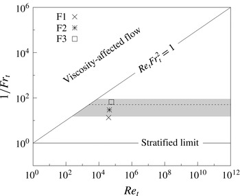
. The significance of this issue can be understood by considering figure 1, which follows from figure 18 of Brethouwer et al. (Reference Brethouwer, Billant, Lindborg and Chomaz2007). In the figure,
 $Re_{t}$
and
 $Fr_{t}$
are the turbulent Reynolds and Froude numbers with the generic horizontal length scale
 $L_{h}$
of (1.1) equated to the turbulence length scale
 $$\begin{eqnarray}L_{t}=A{u_{h}^{\prime }}^{3}/\unicode[STIX]{x1D716}\end{eqnarray}$$
and the generic
 $U_{h}$
defined as the r.m.s. horizontal velocity,
 $u_{h}^{\prime }$
, so that
 $$\begin{eqnarray}Fr_{t}\equiv \frac{u_{h}^{\prime }}{L_{t}N}\quad \text{and}\quad Re_{t}\equiv \frac{u_{h}^{\prime }L_{t}}{\unicode[STIX]{x1D708}}.\end{eqnarray}$$
In the definition of
 $L_{t}$
,
 $A$
is a constant of order unity and
 $\unicode[STIX]{x1D716}$
is the dissipation rate of turbulent kinetic energy. The threshold for the LAST regime, as defined by Brethouwer et al. (Reference Brethouwer, Billant, Lindborg and Chomaz2007) assuming
 $A=1$
, is
 $Fr_{t}\approx 0.02$
, as indicated by a dashed line in the figure. The grey band indicates the uncertainty in this threshold taking into account that
 $A$
in isotropic homogeneous turbulence ranges between 0.4 and 1.81 (Sreenivasan Reference Sreenivasan1998), and that
 $A$
is observed to be as low as
 $0.3$
in stratified turbulence (Maffioli & Davidson Reference Maffioli and Davidson2016). The diagonal line is an estimate for the threshold above which turbulence is significantly affected by viscosity. Turbulence is associated with sufficiently large
 $Re_{t}$
, i.e. sufficiently far to the right on this regime diagram. Furthermore, if
 $Fr_{t}$
is sufficiently large, it is to be expected that the effect of stratification becomes insignificant.
Regime diagram in terms of
 $Re_{t}$
and
 $Fr_{t}$
following Brethouwer et al. (Reference Brethouwer, Billant, Lindborg and Chomaz2007). The grey band represents the range of estimates for the lowest value of
 $1/Fr_{t}$
in the LAST regime based on the range for
 $A$
reported in the literature. The dashed line indicates the limit of the LAST regime assuming
 $A=1$
. The three symbols mark the parameter values for the simulations discussed in detail in this paper.

As described in more detail below, in this paper we consider three simulations, which we denote F1, F2 and F3. Their parameters are listed in table 1, and we mark their locations on the regime diagram. We believe that the value of
 $Re_{t}$
chosen for these simulations is sufficiently large for turbulent flow, and we vary
 $Fr_{t}$
so that these simulations straddle the transition from the ‘weakly’ stratified turbulence regime (using the nomenclature of Brethouwer et al. (Reference Brethouwer, Billant, Lindborg and Chomaz2007)) to the ‘strongly’ stratified or LAST regime.
When the inertial scaling assumption inherent in (1.2) is applied to (1.1) with
 $A=1$
, then
 $Re_{b}=\unicode[STIX]{x1D716}/\unicode[STIX]{x1D708}N^{2}$
. We wish to draw a distinction between the formal scaling
 $Re_{b}\gg 1$
required for the asymptotic formulation of the governing equations to describe dynamics in the LAST regime and this inertial scaling, and so we distinguish between
 $Re_{b}$
as defined in (1.1) and the parameter
 $$\begin{eqnarray}Gn\equiv \unicode[STIX]{x1D716}/\unicode[STIX]{x1D708}N^{2}.\end{eqnarray}$$
We use the symbol
 $Gn$
for this parameter (sometimes called the activity parameter) in recognition of Gibson’s seminal work with this quantity and of Gargett’s association of it with the dynamic range available for fully three-dimensional turbulence (Gibson Reference Gibson and Nihous1980; Gargett, Osborn & Nasmyth Reference Gargett, Osborn and Nasmyth1984).
 $Gn$
is widely used to characterise ocean flows within a wide range of stratification strengths, whereas the scaling arguments underlying the definition of
 $Re_{b}$
apply to the LAST regime alone. It is important to appreciate that
 $Gn$
is an appropriate non-dimensional parameter for any turbulent flow in a stratified fluid, yet is not necessarily equivalent to
 $Re_{b}$
unless
 $A=1$
and
 $L_{h}$
, defined rationally for the flow under consideration, is equal to
 $L_{t}$
.
Simulation parameters for the cases considered in this paper. The uniform grid resolution is denoted by
 $\unicode[STIX]{x1D6E5}$
. It should be noted that the Froude number and buoyancy length include a factor of
 $2\unicode[STIX]{x03C0}$
retained in the conversion of buoyancy frequency to buoyancy period, where all quantities have been defined in § 2. See table 1 in Almalkie & de Bruyn Kops (Reference Almalkie and de Bruyn Kops2012b
) for more details.

The parameter range
 $Gn\in [1,100]$
is observed to occur widely in the world’s oceans (Gargett et al.
Reference Gargett, Osborn and Nasmyth1984; Jackson & Rehmann Reference Jackson and Rehmann2014; Salehipour et al.
Reference Salehipour, Peltier, Whalen and Mackinnon2016), and so it is of geophysical interest to investigate this intermediate range further. This intermediate range is also of particular interest as different dynamical regimes have been identified with different ranges of
 $Gn$
. Specifically, turbulence is expected to be suppressed leading to largely quiescent (though not exactly laminar) flow when
 $Gn\sim O(1)$
(Shih et al.
Reference Shih, Koseff, Ivey and Ferziger2005). In the flows considered by Bartello & Tobias (Reference Bartello and Tobias2013), they found that the turbulence dynamics is very sensitive to
 $Gn$
unless
 $Gn$
is larger than order
 $O(10)$
, which is consistent with some of the earliest scaling analyses on the subject (Gargett et al.
Reference Gargett, Osborn and Nasmyth1984; Gibson Reference Gibson1986; Rohr et al.
Reference Rohr, Itsweire, Helland and Atta1988; Itsweire et al.
Reference Itsweire, Koseff, Briggs and Ferziger1993). Such sensitivity is also observed in the results reported in both Hebert & de Bruyn Kops (Reference Hebert and de Bruyn Kops2006a
) and Hebert & de Bruyn Kops (Reference Hebert and de Bruyn Kops2006b
). More recently, de Bruyn Kops (Reference de Bruyn Kops2015) found that the dynamics of stratified flows are different at
 $Gn=48$
and
 $Gn=220$
, which suggests another threshold at
 $Gn\sim O(100)$
, consistent with the findings of Shih et al. (Reference Shih, Koseff, Ivey and Ferziger2005) and Salehipour & Peltier (Reference Salehipour and Peltier2015).
Although it is clearly not possible to characterise all turbulent stratified flows, particularly in the presence of shear, in terms of a single parameter, as discussed recently by, for example, Maffioli, Brethouwer & Lindborg (Reference Maffioli, Brethouwer and Lindborg2016) and Salehipour et al. (Reference Salehipour, Peltier, Whalen and Mackinnon2016), there are subtleties concerned with spatio-temporal averaging of flow characteristics. Specifically, it is inevitable that the turbulent dissipation rate will vary in space and time, and sufficiently strongly stratified turbulent flow appears to be generically spatio-temporally intermittent. This observation raises a significant implicit issue with the definition of
 $Gn$
(1.4) which must be appreciated. Even in a flow where it is possible to define a single (time-independent) buoyancy frequency
 $N$
, any calculation of
 $Gn$
will thus require the determination of some appropriate domain over which
 $\unicode[STIX]{x1D716}$
is averaged. Typically, the studies just cited considered globally averaged measures of stratification strengths (i.e.
 $N$
) and turbulence characteristics (i.e.
 $\unicode[STIX]{x1D716}$
) to describe a flow. Here, motivated by the clear spatio-temporal variability of stratified turbulence flow, we investigate whether it is possible to subdivide such a flow in a rational, quantitative and robust fashion into different regions with qualitatively different turbulence and mixing properties.
Therefore, we wish to test two inter-related hypotheses. Our first hypothesis is that it is possible to use the density field to categorise a general flow into three characteristic types of regions: ‘quiescent regions’, where an appropriately locally averaged
 $Gn\sim O(1)$
, ‘intermittent layers’, where
 $Gn\sim O(10)$
, and ‘turbulent patches’, where
 $Gn\gtrsim O(100)$
. For widest possible applicability, it is important that this sorting is useful for both ‘strongly’ and ‘weakly’ stratified turbulent flows, i.e. for general turbulent flows whether or not they may be considered to be in the asymptotic LAST regime. Our second hypothesis is that each of these three regions is associated with qualitatively different, yet largely generic, local flow dynamics. If these hypotheses are validated, we will then be in a position to conjecture that at least some of the observed and previously reported sensitivity of the properties of ‘weakly’ or ‘strongly’ stratified turbulence to reported values of
 $Gn$
is due to the fact that the flows are instantaneous assemblages of such different flow subregions with different dynamical properties in (typically) time-varying proportions. Our conjecture, if true, would imply that the overall dynamics of any particular flow can be more clearly understood by quantifying the proportion of the flow domain at any particular instant that is occupied by regions of these three broad types characterised by their values of
 $Gn$
, determined essentially by averaging locally the dissipation rate over the individual subregion, rather than globally over the whole flow domain.
Clearly, central to the hypotheses is the requirement for robust identification of such individual subregions. Here, we present just such an identification method based on the space-filtered probability density of the vertical derivative of the fluid density. In this paper, we exclusively demonstrate this method by consideration of data from numerical simulation. Nevertheless, it is important to stress that a particular attraction of this method, unlike ones based on enstrophy for example (see Watanabe et al. Reference Watanabe, Riley, de Bruyn Kops, Diamessis and Zhou2016), is that it could, in principle, be applied to experimental data if the instantaneous density field at some resolution is captured on a horizontal–vertical plane using laser-induced fluorescence (LIF).
To test our hypotheses, the rest of this paper is organised as follows. In § 2, we briefly describe three simulations with different characteristic horizontal Froude numbers, and thus different relative strengths of overall stratification. We also present contour plots that suggest that the different flows are indeed assemblages of qualitatively different subregions in varying proportions. In § 3, we present our method based on the cumulative filtered distribution of the local density gradient. We apply this method to our simulation data in § 4, finding that both of our hypotheses appear to be consistent with our data. Finally, we present our conclusions in § 5.
2 Direct numerical simulations
We consider statistically stationary direct numerical solutions of the Navier–Stokes equations subject to the non-hydrostatic Boussinesq assumption and with unity Prandtl number. We impose periodic boundary conditions in all directions. The flow has no mean shear, but a uniform background ambient stratification is maintained so that the flow statistics are homogeneous and independent of (horizontal) direction. We maintain quasistationarity by forcing the largest scales of the horizontal velocities to have a prescribed spectrum using the method denoted Rf in Rao & de Bruyn Kops (Reference Rao and de Bruyn Kops2011). Local shear is induced by random low-energy perturbations to the horizontal velocity components at small vertical wavenumbers. The prescribed spectrum for the forcing is obtained by repeating the simulations of Lindborg (Reference Lindborg2006) using his forcing method, and so the current flows are very similar in structure to those in that paper.
As already noted, parameters for the three simulations, which we denote F1, F2 and F3, are listed in table 1. Since the largest scales of the horizontal velocities are forced to the same target spectrum for all simulations, and the viscosities are the same, the key difference between the simulations is the magnitude of the ambient density gradient, which allows us to investigate the transition from the weakly stratified to the LAST regime, as shown in figure 1. (See Almalkie & de Bruyn Kops (Reference Almalkie and de Bruyn Kops2012b
) and de Bruyn Kops (Reference de Bruyn Kops2015) for more detailed discussion of these simulations.) We define the buoyancy (
 $L_{b}$
), Ozmidov (
 $L_{o}$
), Taylor (
 $\unicode[STIX]{x1D706}$
) and Kolmogorov (
 $L_{k}$
) length scales in the usual way in terms of the r.m.s. velocity
 $u^{\prime }$
, the dissipation rate of turbulence kinetic energy
 $\unicode[STIX]{x1D716}$
and the buoyancy frequency
 $N\equiv \sqrt{-g/\unicode[STIX]{x1D70C}_{0}\,\text{d}\bar{\unicode[STIX]{x1D70C}}/\text{d}x_{3}}$
, each of which is averaged over the entire domain. In particular, in these flows it is natural to use such a global buoyancy frequency in the calculation of
 $Gn$
, although the dissipation rate typically has large spatial variation. Here,
 $g$
is the gravitational acceleration antiparallel to the
 $x_{3}$
coordinate, and the total density
 $\unicode[STIX]{x1D70C}_{t}$
is the sum of reference, ambient and fluctuating components, i.e.
 $\unicode[STIX]{x1D70C}_{t}=\unicode[STIX]{x1D70C}_{0}+\bar{\unicode[STIX]{x1D70C}}(x_{3})+\unicode[STIX]{x1D70C}(\boldsymbol{x},t)$
. The fluctuating density
 $\unicode[STIX]{x1D70C}$
satisfies periodic boundary conditions. The factor of
 $2\unicode[STIX]{x03C0}$
is retained in the definition of
 $L_{b}$
.
The direct numerical simulations are computed using a Fourier pseudospectral method. A fractional step method with the Adams–Bashforth scheme is used for time integration. The nonlinear term in the momentum equation is computed in rotational form, and the corresponding term in the internal energy equation is computed in convective and conservation forms on alternating time steps to approximate the skew-symmetric form and ensure energy conservation. The simulations are fully dealiased by truncating the Fourier series. The domain is collocated on
 $8192\times 8192\times N_{z}$
uniformly spaced grid points, where
 $N_{z}$
is the number of grid points in the vertical dimension, as listed in table 1.
As discussed in the introduction, we are interested in the identification of regions of dynamically distinct turbulence. It has been proposed by Watanabe et al. (Reference Watanabe, Riley, de Bruyn Kops, Diamessis and Zhou2016) that the potential enstrophy
 $\unicode[STIX]{x1D6F1}\equiv (\unicode[STIX]{x1D74E}\boldsymbol{\cdot }\unicode[STIX]{x1D735}\unicode[STIX]{x1D70C}_{t})^{2}$
, where
 $\unicode[STIX]{x1D74E}$
is the vorticity, is effective in distinguishing turbulence from internal waves. A vertical plane though the
 $\unicode[STIX]{x1D6F1}$
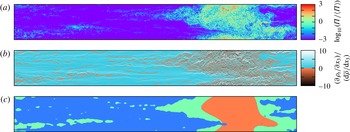
field in the most strongly stratified simulation F3 is shown in figure 2(a). Qualitatively, layered structures can be seen towards the left of the image, whereas a patch of turbulence dominates the flow to the right. As we discuss in more detail below, only a small fraction (less than 5 %) of the volume of this flow is occupied by such patches, but this plane has been carefully chosen to show the full variety of regions that arise and can be identified by our method in a stratified turbulent flow. Figure 2(b) illustrates
 $(\unicode[STIX]{x2202}\unicode[STIX]{x1D70C}_{t}/\unicode[STIX]{x2202}x_{3})/(\text{d}\bar{\unicode[STIX]{x1D70C}}/\text{d}x_{3})$
for the same plane, with a colour map chosen to emphasise the sign of
 $(\unicode[STIX]{x2202}\unicode[STIX]{x1D70C}_{t}/\unicode[STIX]{x2202}x_{3})/(\text{d}\bar{\unicode[STIX]{x1D70C}}/\text{d}x_{3})$
. The visual similarity between figures 2(a) and 2(b) is one of the two motivations of our identification method, the other being the practical issue that planar data on the instantaneous density field, and in particular point-wise vertical gradients of the density field, are more accessible in the laboratory than all of the components of the velocity gradient tensor necessary to determine the enstrophy.
A vertical slice through case F3 illustrating (a) the logarithm of the potential enstrophy normalised by its domain average, (b)
 $\unicode[STIX]{x2202}\unicode[STIX]{x1D70C}_{t}/\unicode[STIX]{x2202}x_{3}/\text{d}\bar{\unicode[STIX]{x1D70C}}/\text{d}x_{3}$
and (c) the results of the flow classification as implemented in § 3. The colouring in (b) highlights the convectively unstable fluid elements in red. The colouring in (c) corresponds to the region classification, where red indicates a turbulent patch region, green an intermittent layer region and blue a quiescent flow region.

3 Methodology
Our proposed method for identifying dynamically different regions in stratified turbulence generalises the method discussed by Hedley & Keffer (Reference Hedley and Keffer1974) for making what they refer to as ‘turbulent/non-turbulent decisions’. This three-stage method involves first choosing a diagnostic field variable
 $\unicode[STIX]{x1D719}(\boldsymbol{x})$
, then computing a detector function
 $Q(\unicode[STIX]{x1D719},\boldsymbol{x})$
to identify values of the diagnostic field variable using a characteristic filter size
 $\ell$
to remove the effects of internal intermittency, and finally discriminating between turbulent and non-turbulent regions by identifying as turbulent regions where
 $Q\geqslant Q^{\ast }$
for some threshold value
 $Q^{\ast }$
. These three stages have been used effectively to distinguish between two flow regions with different characteristics (e.g. Kuo & Corrsin Reference Kuo and Corrsin1971; Antonia Reference Antonia1981; Nolan & Zaki Reference Nolan and Zaki2013). However, we hypothesise that stratified turbulent flow can be subdivided into three dynamically different flow regions, and so it is necessary to use two different filter widths, as we detail below.
Watanabe et al. (Reference Watanabe, Riley, de Bruyn Kops, Diamessis and Zhou2016) report that both the enstrophy and the potential enstrophy are needed to identify the turbulent/non-turbulent interface in stratified wakes. However, since our purpose here is not to determine precisely the edge of a turbulent region but rather to compute a robust (and substantially less computationally demanding) detector function of a diagnostic variable indicative of sufficiently spatially extended and connected turbulent regions, we choose the diagnostic field variable to be defined as
 $\unicode[STIX]{x1D719}=\unicode[STIX]{x2202}\unicode[STIX]{x1D70C}_{t}(\boldsymbol{x})/\unicode[STIX]{x2202}x_{3}$
. It is at least plausible that active turbulence will lead to a high probability of inverted density gradients, and so we believe that
 $\unicode[STIX]{x1D719}>0$
should be a good indicator of turbulence.
Not least due to the inherent range of scales associated with turbulent motions, the inherent non-locality of turbulence requires that any suitable identification method to distinguish turbulent patches, intermittent layers and quiescent flow regions must depend on an appropriate filter function
 $G(\boldsymbol{x};\ell )$
. For the results shown here,
 $G$
is the Gaussian function with variance
 $\ell$
, but a spherical filter with diameter
 $\ell$
yields comparable results. Furthermore, since we wish to be able to distinguish between two different types of turbulent regions, corresponding to anisotropic intermittent layers (in the sense that the horizontal extent of such layers is typically much larger than the vertical extent) and more three-dimensional turbulent patches, we choose two different filter widths,
 $\ell _{1}$
and
 $\ell _{2}$
, in an attempt to capture the different geometries of the two types of regions. This leads to the filtered density functions
 $q_{i}(\boldsymbol{x},\unicode[STIX]{x1D719}^{\prime })$
and the associated cumulative filtered density functions (c.f.d.f.)
 $Q_{i}(\boldsymbol{x})$
, defined as
 $$\begin{eqnarray}q_{i}(\boldsymbol{x},\unicode[STIX]{x1D719}^{\prime })=\int _{-\infty }^{\infty }\unicode[STIX]{x1D6FF}\left[\unicode[STIX]{x1D719}^{\prime }-\unicode[STIX]{x1D719}(\boldsymbol{x}-\boldsymbol{r})\right]G(\boldsymbol{r};\ell _{i})\,\text{d}\boldsymbol{r},\quad Q_{i}(\boldsymbol{x})=\int _{\unicode[STIX]{x1D6F7}_{i}}^{\infty }q_{i}(\boldsymbol{x},\unicode[STIX]{x1D719}^{\prime })\,\text{d}\unicode[STIX]{x1D719}^{\prime },\end{eqnarray}$$
where
 $\unicode[STIX]{x1D6FF}$
is the Dirac
 $\unicode[STIX]{x1D6FF}$
-function,
 $\boldsymbol{r}$
is a dummy variable for the convolution,
 $\ell _{i}$
are the filtering scales,
 $\unicode[STIX]{x1D6F7}_{i}$
is an appropriate upper limit and
 $i=1,2$
. Since the diagnostic field variable
 $\unicode[STIX]{x1D719}$
is the vertical derivative of the total density, we set
 $\unicode[STIX]{x1D6F7}_{1}=\unicode[STIX]{x1D6F7}_{2}=0$
, so that the
 $Q_{i}$
give the fraction of locations within the filter region at which the density gradient is unstable.
To identify the critical lower threshold for the existence of turbulence (in either layer or patch regions), we set the small filter length equal to the Taylor length scale,
 $\ell _{1}=\unicode[STIX]{x1D706}$
, based on the observation that there appears to be power-law scaling of the internal intermittency at this length scale even at the relatively modest Reynolds numbers accessible in simulations (Almalkie & de Bruyn Kops Reference Almalkie and de Bruyn Kops2012a
; de Bruyn Kops Reference de Bruyn Kops2015). Kuo & Corrsin (Reference Kuo and Corrsin1971) suggest a filter width of
 $10L_{k}$
, which corresponds to approximately
 $\unicode[STIX]{x1D706}/4$
for our data, and our conclusions do not change qualitatively if this (smaller) length scale is used for the filter length
 $\ell _{1}$
. To identify ‘patch’ regions of overturning with vertical extent greater than that typical of intermittent layers, we choose the filter length
 $\ell _{2}=L_{b}$
, the buoyancy length scale, as this scale is thought to characterise the thickness of layers in the ‘strongly stratified’ or LAST regime (Billant & Chomaz Reference Billant and Chomaz2001; Brethouwer et al.
Reference Brethouwer, Billant, Lindborg and Chomaz2007).
The final stage in the identification method is the determination of appropriate threshold values
 $Q_{1}^{\ast }$
and
 $Q_{2}^{\ast }$
for the two detector functions. We denote by
 $I_{1}$
and
 $I_{2}$
the sets of all points in the domain where
 $Q_{1}\geqslant Q_{1}^{\ast }$
and
 $Q_{2}\geqslant Q_{2}^{\ast }$
respectively. Since the buoyancy length exceeds the Taylor length,
 $L_{b}>\unicode[STIX]{x1D706}$
, for all cases,
 $I_{2}$
is the set of regions with density inversions down to a relatively large vertical length scale, whereas
 $I_{1}$
is the set of regions with density inversions down to a relatively small vertical scale. It is thus natural to identify energetic turbulent patches as the set of points
 $I_{P}$
contained in both
 $I_{1}$
and
 $I_{2}$
, while intermittent layers can be identified as the set of points
 $I_{L}$
that are in
 $I_{1}$
but are not in
 $I_{2}$
. Quiescent regions can then be defined as all the remaining points, i.e. the set of points
 $I_{Q}$
that are in neither
 $I_{1}$
nor
 $I_{2}$
, and so
 $$\begin{eqnarray}\displaystyle I_{1}\equiv \{\boldsymbol{x}|Q_{1}\geqslant Q_{1}^{\ast }\},\quad I_{2}\equiv \{\boldsymbol{x}|Q_{2}\geqslant Q_{2}^{\ast }\}, & & \displaystyle\end{eqnarray}$$
 $$\begin{eqnarray}\displaystyle I_{P}\equiv I_{1}\cap I_{2},\quad I_{L}\equiv I_{1}\cap I_{2}^{C},\quad I_{Q}\equiv I_{1}^{C}=(I_{P}\cup I_{L})^{C}, & & \displaystyle\end{eqnarray}$$
where
 $(\cdot )^{C}$
indicates a complement. Within the framework of strongly and weakly stratified turbulence (e.g. Brethouwer et al.
Reference Brethouwer, Billant, Lindborg and Chomaz2007),
 $Q_{1}^{\ast }$
and
 $Q_{2}^{\ast }$
distinguish weakly stratified regions from strongly stratified layers, and
 $Q_{1}^{\ast }$
further distinguishes the quiescent (though not necessarily completely laminar) regions within the layers, which are characteristic of strongly stratified turbulence in the LAST regime, cf. Hebert & de Bruyn Kops (Reference Hebert and de Bruyn Kops2006a
, figure 5), Brethouwer et al. (Reference Brethouwer, Billant, Lindborg and Chomaz2007, figure 8) and Bartello & Tobias (Reference Bartello and Tobias2013, figure 19).
4 Results
The method discussed in § 3 allows for different flow regions to be identified given threshold values
 $Q_{1}^{\ast }$
and
 $Q_{2}^{\ast }$
. We analyse the simulation data to identify (if possible) values for
 $Q_{1}^{\ast }$
and
 $Q_{2}^{\ast }$
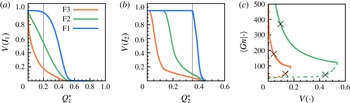
for which the regions identified as patches, layers and quiescent regions are at most weakly sensitive to those threshold values. In figures 3(a) and 3(b) respectively, we plot the fractions
 $V(I_{1})$
and
 $V(I_{2})$
of the total flow volume identified to be in the sets
 $I_{1}$
and
 $I_{2}$
for the three different simulations under consideration as functions of the threshold values
 $Q_{1}^{\ast }$
and
 $Q_{2}^{\ast }$
. Appropriate relatively robust values of these thresholds can be determined by considering the blue lines, which represent the data for the least strongly stratified simulation, F1, which is, unsurprisingly, in the ‘weakly stratified’ regime in figure 1. In simulation F1, virtually all of the filtered volumes include significant overturning. This simulation is used to define turbulent patch regions with
 $V(I_{1})\simeq 1$
and
 $V(I_{2})\simeq 1$
so that the patch region nearly fills the volume. Based on figures 3(a,b), we set
 $Q_{1}^{\ast }$
and
 $Q_{2}^{\ast }$
to the largest possible values that maintain
 $V(I_{1})\simeq 1$
and
 $V(I_{2})\simeq 1$
. Larger values of
 $Q_{1}^{\ast }$
and
 $Q_{2}^{\ast }$
are preferred since this results in a detection method that is more sensitive to changes in flow behaviour. Therefore, we choose these values (marked with vertical lines in the figures) as appropriate thresholds to identify turbulent regions (either layers or patches) in the other two flows, which clearly also contain quiescent regions. Generally, the thresholds may be chosen at the edge of a region insensitive to
 $Q_{1}^{\ast }$
and
 $Q_{2}^{\ast }$
, and not necessarily where
 $V(I_{1})$
and
 $V(I_{2})$
achieve approximate unity.
(a) The fraction of the flow volume
 $V(I_{1})$
as a function of the threshold
 $Q_{1}^{\ast }$
and (b)
 $V(I_{2})$
in set
 $I_{2}$
as a function of the threshold
 $Q_{2}^{\ast }$
. The thin vertical lines show the chosen values
 $Q_{1}^{\ast }=0.2$
and
 $Q_{2}^{\ast }=0.35$
used in our analysis. (c) Variation of
 $Gn$
as a function of the volume identified with patch regions (solid lines) and layer regions (dashed lines) as the parameter
 $Q_{2}^{\ast }$
is varied. The symbols correspond with the volumes in table 2.

Using these chosen values, it is now possible to identify the three different regions, which we hypothesise have different dynamical properties, using (3.2). As an example for the most strongly stratified case F3, such an identification on a particular plane is shown in figure 2(c). It is important to remember that our proposed identification method is not intended to classify the turbulence properties of every single point in the flow independently, but rather to characterise somewhat more extended regions of the flow in terms of the proportion of the region that has inverted density gradients over physically motivated length scales. Nevertheless, as is apparent in the figure, our method appears to be able to identify the layered structures extending to either side of the patch, as well as the intrusion of a quiescent region into the lower left edge of the patch.
A further test of the sensitivity of our results to the threshold value
 $Q_{2}^{\ast }$
is the variation of the conditionally averaged
 $Gn$
in each type of region as a function of the volume identified with regions of that type. We define the conditional
 $Gn$
for regions
 $I=I_{P},I_{L},I_{Q}$
as
 $\langle Gn|I\rangle \equiv \langle \unicode[STIX]{x1D716}_{0}|I\rangle /\unicode[STIX]{x1D708}\langle N_{0}^{2}|I\rangle$
, where the notation
 $\langle \cdot |I\rangle$
denotes a conditional average over the set indicated by
 $I$
. Here,
 $\unicode[STIX]{x1D716}_{0}$
is the local dissipation rate of kinetic energy and
 $N_{0}\equiv \sqrt{-g/\unicode[STIX]{x1D70C}_{0}~\unicode[STIX]{x2202}\unicode[STIX]{x1D70C}_{t}(\boldsymbol{x})/\unicode[STIX]{x2202}x_{3}}$
. The conditional
 $Gn$
over the points identified with each region is plotted in figure 3(c) for the full range of possible values of
 $Q_{2}^{\ast }$
. We do not show curves for case F1 because this case is used to determine the appropriate threshold values, and we wish to test the robustness of this determination.
To aid in interpreting figure 3(c), it should be noted that for case F2 with
 $Q_{1}^{\ast }=0.2$
, approximately 55 % of the volume is identified as turbulent, and the average
 $Gn$
for the turbulent volume is approximately 120. The right end of the solid green curve in figure 3(c) corresponds to
 $Q_{2}^{\ast }$
being chosen so as to define all of the turbulence as patches. The right end of the dashed green line corresponds to a different value of
 $Q_{2}^{\ast }$
such that all of the turbulence is identified as layers. Neither of these values of
 $Q_{2}^{\ast }$
, though, results in classifications consistent with contour plots for F2 similar to figure 2(a). For almost any intermediate value of
 $Q_{2}^{\ast }$
chosen,
 $Gn\sim O(10)$
in the layers and
 ${\sim}O(100)$
in the patches. In fact, the long plateau in the dashed green line indicates that the statement
 $Gn\sim O(10)$
for layers is very insensitive to the volume fraction identified as layers based on the choice of
 $Q_{2}^{\ast }$
. For all of the cases,
 $Gn\sim O(100)$
is completely insensitive to
 $Q_{2}^{\ast }$
. The numerical values for the conditionally averaged values of
 $Gn$
in the various regions and simulations when the thresholds are set to
 $Q_{1}^{\ast }=0.2$
and
 $Q_{2}^{\ast }=0.35$
are given in table 2.
It is apparent that the first hypothesis set forth in the introduction is validated, i.e. three elemental regions can be identified using the density field, which are characterised by distinct values of
 $Gn$
. It is also clear that this identification is largely robust with respect to the choice of threshold values, and also to the particular turbulent regime of the flow under consideration.
We now turn our attention to the second hypothesis, i.e. that patches, layers and quiescent regions are associated with qualitatively different, yet largely generic, local flow dynamics. As an example test of this hypothesis, we apply our method to interpret the dissipation and irreversible mixing characteristics of the flows. de Bruyn Kops (Reference de Bruyn Kops2015) showed that the shapes of the probability density functions (p.d.f.s) of the local dissipation rate of turbulence kinetic energy,
 $\unicode[STIX]{x1D716}_{0}$
, and the local rate at which available potential energy is lost due to molecular mixing,
 $\unicode[STIX]{x1D712}_{0}$
, depend strongly on the value of the domain-averaged
 $Gn$
. In particular, for flows with sufficiently large values of
 $Gn$
, e.g. as in case F1, the p.d.f.s are very similar to those for isotropic homogeneous turbulence with a mean (passive) scalar gradient.
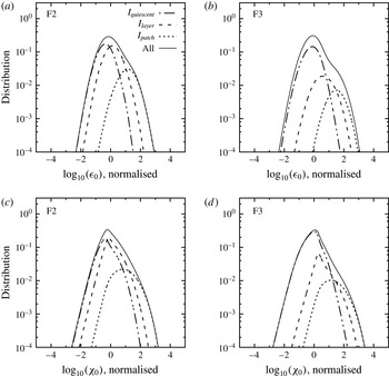
The p.d.f.s of the logarithms of the local kinetic energy dissipation rate
 $\unicode[STIX]{x1D716}_{0}$
and the scalar mixing rate
 $\unicode[STIX]{x1D712}_{0}$
normalised by their means and variances. The solid curve in each panel is a p.d.f. The remaining curves sum to the solid curve but are not p.d.f.s themselves.

In figure 4, these p.d.f.s are plotted along with the separated contributions from the patch, layer and quiescent regions. We see that virtually all of the high dissipation rates and high mixing rates occur in patch regions, with, in particular, the evident ‘shoulder’ in the p.d.f. of dissipation at high values being associated with the patch regions. Indeed, in absolute terms, the majority of the dissipation and mixing occurs in patch regions, as shown in table 2, even for the flow case F3, where less than 5 % of the flow volume is identified as being in turbulent patch regions. (As already noted, the plane chosen for figure 2 was carefully chosen to show all three kinds of regions: patches, layers and quiescent regions.)
Fundamentally, the identification method proposed here allows us to identify regions where dissipation and mixing have qualitatively different character, thus confirming our second hypothesis. Further dynamical differences between cases F1, F2 and F3, such as markedly differing transfer rate spectra and differing relative importance of vertical shear to the dissipation rate of kinetic energy, are reported in Almalkie & de Bruyn Kops (Reference Almalkie and de Bruyn Kops2012b ) and de Bruyn Kops (Reference de Bruyn Kops2015).
Local
 $Gn$
averaged for the points in each region, the local kinetic and available potential energy dissipation rates averaged for the points in each region as ratios of their totals in the domain, and the volume percentage associated with each region.

These simulations are similar in some respects to those of Lindborg (Reference Lindborg2006), although we have used a different forcing protocol to speed convergence. Lindborg prescribed the average dissipation rate, irrespective of the organisation of the flow into ‘patches’, ‘layers’ or ‘quiescent regions’. This is consistent with the concept that the small scales of turbulence adjust to the energy being fed from the larger scales. In the current simulations, the average dissipation rate over the entire flow domain is not prescribed, but it is comparable for all three cases. Nevertheless, the transfer rate spectra are very different between the cases (Almalkie & de Bruyn Kops Reference Almalkie and de Bruyn Kops2012b ), which is evidence that the flows dynamically adjust to dissipate the energy provided by the (forced) large scales. This is clear evidence that the flows adjust to satisfy the dissipation rate constraint through modifying the relative proportions of the flow that are active and closer to isotropic at least geometrically (i.e. patches), anisotropic (with high aspect ratio) and intermittent (i.e. layers) and quiescent, consistently with the externally imposed stratification.
5 Conclusions
In summary, we have defined a method for identifying distinct dynamical regions in a stratified flow that is robust to the choice of threshold values. By applying it to simulation data, it is observed that by far the majority of dissipation and mixing occurs in regions identified as patches of turbulence, even when these regions comprise a very small fraction of the total volume. Interestingly, the patches in simulation F3 appear to be very similar dynamically to the patches in F1, in terms of their dissipation and mixing properties. The central stabilising effect of stratification, associated with F3 being in the strongly stratified or LAST regime and F1 being in the weakly stratified regime as classified by Brethouwer et al. (Reference Brethouwer, Billant, Lindborg and Chomaz2007), does not appear to be that turbulence when it occurs is always less intense. Rather, ‘strong’ stratification appears to reduce the proportion of the flow that is in intensely turbulent patches, as the flow adjusts to have significant proportions of the flow domain identifiable as intermittent (and more weakly turbulent, at least as quantified by the appropriate local value of
 $Gn$
) geometrically anisotropic layers, or indeed essentially quiescent regions.
We also believe that our proposed method is well suited to the identification of intensely mixing turbulent patches from laboratory density measurements using LIF at sufficiently high spatial and temporal resolution, particularly since it is not necessary to resolve the very smallest scale of structures in the density field, but rather just identify regions of local inversion. This identification appears to be independent of where the flow parameters are located in the regime diagram figure 1 (following Brethouwer et al. (Reference Brethouwer, Billant, Lindborg and Chomaz2007)); in particular, the identification appears to be robust (for sufficiently high
 $Re_{h}$
) across the weakly stratified and LAST regimes. Furthermore, our result that the turbulence in (identifiable) patches is largely similar for the three simulations considered appears to explain the p.d.f.s of mixing and dissipation rates in the literature.
Finally, we propose that this methodology could be applied to analyse in detail the characteristics of turbulence and mixing objectively in highly spatio-temporally intermittent stratified flows with a wide range of flow parameters, including, for example, flows with large-scale shear, as our method is inherently local in its analysis of the density field structure. Specifically, it could be used to understand other published results which appear to be very sensitive to small changes in flow configuration or bulk properties. We conjecture that such sensitivity is due to variations in the relative proportions of the different types of regions, with, for example, a slight reduction in the proportion of the volume that can be classified as a turbulent patch region leading to a marked reduction in the total amount of dissipation and mixing occurring within the flow.
Acknowledgements
The research activities of G.D.P. and S.dB.K. were funded by the US Office of Naval Research via grant N00014-15-1-2248. Additional support to G.D.P. and S.dB.K. was provided from the UK Engineering and Physical Sciences Research Council grant EP/K034529/1 entitled ‘Mathematical Underpinnings of Stratified Turbulence’, which also funds the research activity of J.R.T. and C.P.C. H.S. gratefully acknowledges the award of a Crighton Fellowship at the Department of Applied Mathematics & Theoretical Physics, University of Cambridge. High-performance computing resources were provided through the US Department of Defense High Performance Computing Modernization Program by the Army Engineer Research and Development Center and the Army Research Laboratory under Frontier Project FP-CFD-FY14-007. The data used to construct figures 3 and 4 of this paper are available at http://dx.doi.org/10.17863/CAM.4493.