1. Introduction
Internal hydraulic jumps occur in a variety of situations. River outflows can excite undular bores in the stratified ambient fluid into which they propagate (Nash & Moum Reference Nash and Moum2005). Other examples include atmospheric undular bores, such as the Morning Glory in Australia and Oklahoma, sea breeze fronts and thunderstorm outflows (Rottman & Simpson Reference Rottman and Simpson1989). Internal hydraulic control and jumps can occur in the abyssal ocean as dense water flows over sills between deep basins (Polzin et al. Reference Polzin, Speer, Toole and Schmitt1996; St Laurent & Thurnherr Reference St Laurent and Thurnherr2007; Alford et al. Reference Alford, Girton, Voet, Carter, Mickett and Klymak2013). They also occur in connecting channels such as Gibraltar, where the amount of mixing affects the Mediterranean water properties and in peripheral channels such as Knight Inlet (Farmer & Armi Reference Farmer and Armi1999; Klymak & Gregg Reference Klymak and Gregg2003; Sánchez-Garrido et al. Reference Sánchez-Garrido, Sannino, Liberti, Lafuente and Pratt2011).
Non-rotating internal hydraulic jumps in two-layer flows are the focus of this work. These are relevant in narrow channels with sills, such as Knight Inlet and the Pre-Bosphorus Channel (Gregg & Özsoy Reference Gregg and Özsoy2002; Klymak & Gregg Reference Klymak and Gregg2004). The flow in these channels can often be approximated as a two-layer flow with a chosen isopycnal as the interface. In cases such as the Pre-Bosphorus Channel, two distinct layers are clearly evident in the exchange flow due to the salinity and temperature differences of the source waters (Gregg & Özsoy Reference Gregg and Özsoy2002). The opposing flows also suggest that the effects of ambient vertical shear upstream of a jump could be significant.
Most existing theories treat the flow as two-layered, ignore the mixing and internal dynamics of the jump and use shock-joining theories to match the upstream and downstream conditions (Wood & Simpson Reference Wood and Simpson1984; Klemp, Rotunno & Skamarock Reference Klemp, Rotunno and Skamarock1997; Li & Cummins Reference Li and Cummins1998). The two-layer problem is typically approached by conserving mass and momentum flux through the jump. However, because of the rigid lid imposed at the surface, an additional assumption is then required to close the problem due to the change in surface pressure across the jump. This assumption determines how mechanical energy dissipation within the jump is distributed between the layers. Two-layer model closures to this problem include those by Wood & Simpson (Reference Wood and Simpson1984), which conserves energy in the contracting layer, and Klemp et al. (Reference Klemp, Rotunno and Skamarock1997), which conserves energy in the expanding layer. Li & Cummins (Reference Li and Cummins1998) proposed a model in which the energy loss can be partitioned arbitrarily between the two layers. Recently, Borden & Meiburg (Reference Borden and Meiburg2013b ) proposed an approach based on vorticity conservation across the jump. By integrating the vorticity equation through the jump, they balance the baroclinic production of vorticity in the jump with the downstream flux of vorticity on the vortex sheet between the fluid layers. The appealing aspect of their model is that the apparently arbitrary choice of how to distribute dissipation is replaced with a constraint on the vorticity. This results in dissipation in both layers such that the Bernoulli head difference between the layers is conserved across the jump (Borden & Meiburg Reference Borden and Meiburg2013a ; White & Helfrich Reference White and Helfrich2014). However, in a dissipative turbulent flow, spatial variations in dissipation can lead to production of vorticity within the jump so that the divergence in vorticity advection is not necessarily balanced exactly by baroclinic production (White & Helfrich Reference White and Helfrich2014). Borden & Meiburg (Reference Borden and Meiburg2013b ) also extended this idea to allow a finite thickness shear layer downstream of the jump, and the theory agrees reasonably well with numerical model simulations for flows without upstream shear.
The two-layer studies discussed above have focused primarily on internal bores advancing into a resting two-layer stratification. In many oceanographic situations upstream shear is present and likely important. Examples include jumps in dense overflows (Alford et al. Reference Alford, Girton, Voet, Carter, Mickett and Klymak2013) and exchange flows, such as the Strait of Gibraltar and the Pre-Bosphorus channel (Gregg & Özsoy Reference Gregg and Özsoy2002; Klymak & Gregg Reference Klymak and Gregg2004; Sánchez-Garrido et al. Reference Sánchez-Garrido, Sannino, Liberti, Lafuente and Pratt2011), that have upstream shear by definition. However, the effect of upstream shear has not been fully investigated in the layer models. Klemp et al. (Reference Klemp, Rotunno and Skamarock1997) suggested that with sufficient upstream shear, their closure of energy conservation in the expanding layer might fail, and that the Wood & Simpson (Reference Wood and Simpson1984) closure might be more appropriate.
In an effort to address the issue we explore the behaviour of two-layer jumps with upstream shear using the energy closures considered by Wood & Simpson (Reference Wood and Simpson1984), Klemp et al. (Reference Klemp, Rotunno and Skamarock1997), and the Borden & Meiburg (Reference Borden and Meiburg2013b ) vorticity conservation model. We also extend the work of Borden, Meiburg & Constantinescu (Reference Borden, Meiburg and Constantinescu2012), which includes a downstream shear layer and resulting inter-layer energy exchange, to include upstream shear. The physically allowable solution space of the two-layer theories is carefully identified by consideration of the stability of the flow to long interfacial waves and the requirement that energy must be lost across the jump.
These two-layer theories neglect non-hydrostatic processes, turbulence, and mixing within the hydraulic transition between the upstream and downstream states. These models can be modified to parameterize the effects of mixing (cf. Borden & Meiburg Reference Borden and Meiburg2013b ). However, these modifications do not directly incorporate the detailed dynamics within the jumps and need to be tested. Since understanding the role of mixing is one of the primary motivations for studying internal jumps, numerical simulations of internal hydraulic jumps are performed with a non-hydrostatic numerical model that allows continuous density and velocity profiles and turbulent mixing. The numerical results are then compared with the predictions from the two-layer theories.
2. Two-layer theories
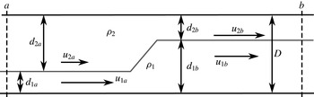
The two-layer flow set-up is shown in figure 1. Two immiscible layers of distinct densities,
 ${\it\rho}_{i}$
, flow between rigid horizontal boundaries separated by a constant distance
 $D$
. The lower layer undergoes a sudden expansion, or hydraulic jump. In this work, the lower layer is always taken to be shallower upstream and thus the expanding layer. However, for Boussinesq flows, the results also apply to hydraulic jumps with expanding upper layers. Each layer has a depth,
 $d_{i}$
, and velocity,
 $u_{i}$
, which change across the jump. The jump is considered in the frame of reference moving with the jump, so the layer velocities are relative to the speed of the jump and the governing equations are stationary. The subscript
 $i=1\;(2)$
indicates the lower (upper) layer. The subscript
 $a$
(
 $b$
) indicates upstream (downstream) of the jump, corresponding to the vertical sections similarly labelled in figure 1.
Problem set-up.

The two-layer theories explored by Wood & Simpson (Reference Wood and Simpson1984), Klemp et al. (Reference Klemp, Rotunno and Skamarock1997), and Li & Cummins (Reference Li and Cummins1998) are shock-joining models based on conservation of layer mass and total momentum flux across the jump (cf. Klemp et al. Reference Klemp, Rotunno and Skamarock1997),
 $$\begin{eqnarray}\displaystyle & \displaystyle [d_{i}u_{i}]_{a}^{b}=0,\quad \text{for }i=1,2, & \displaystyle\end{eqnarray}$$
 $$\begin{eqnarray}\displaystyle & \displaystyle \left[\int _{0}^{D}(p+{\it\rho}u^{2})\,\text{d}z\right]_{a}^{b}=0, & \displaystyle\end{eqnarray}$$
where
 $[\cdot ]_{a}^{b}$
indicates the difference across the bore (downstream minus upstream). The volume flow rate per unit width in each layer is
 $q_{i}=d_{i}u_{i}$
and
 $p(z)$
is the pressure. The theories assume that there is no mixing, so the density in each layer is constant, and the detailed dynamics within the jump are ignored. The problem is considered in the frame of reference moving with the bore. If the upstream conditions are known, then these three equations should allow one to solve for the downstream conditions,
 $u_{1d}$
,
 $u_{2d}$
,
 $d_{1d}$
,
 $d_{2d}$
, using the rigid-lid assumption,
 $d_{1}+d_{2}=D$
, and assuming the pressure is hydrostatic in the uniform regions up- and downstream of the jump:
 $$\begin{eqnarray}p=\left\{\begin{array}{@{}ll@{}}p_{s}+g{\it\rho}_{2}(D-z), & d_{1}<z<d_{2},\\ p_{s}+g{\it\rho}_{2}d_{2}+g{\it\rho}_{1}(D-d_{2}-z), & 0<z<d_{1}.\end{array}\right.\end{eqnarray}$$
However, the surface pressure,
 $p(z=D)=p_{s}$
, is unknown and can change across the jump. This introduces an additional unknown,
 $[p_{s}]_{a}^{b}$
, requiring another constraint to close the system. Wood & Simpson (Reference Wood and Simpson1984) assumed conservation of energy flux in the upper (contracting) layer, which is equivalent to conserving the Bernoulli function along
 $z=D$
. With this assumption,
 $$\begin{eqnarray}[E_{2}]_{a}^{b}=\left[\int _{d_{1}}^{D}u\left(p+{\it\rho}\frac{u^{2}}{2}+{\it\rho}gz\right)\text{d}z\right]_{a}^{b}=q_{2}[p_{s}+{\it\rho}_{2}u_{2}^{2}]_{a}^{b}=0,\end{eqnarray}$$
and
 $$\begin{eqnarray}[p_{s}]_{a}^{b}=-[{\it\rho}_{2}u_{2}^{2}]_{a}^{b}.\end{eqnarray}$$
After eliminating
 $u_{2b}$
, the closed set of equations for the unknown
 $d_{2b}$
are
 $$\begin{eqnarray}D[p_{s}]_{a}^{b}+\left[({\it\rho}_{1}-{\it\rho}_{2})\frac{g}{2}(d_{1b}^{2}-d_{1a}^{2})+{\it\rho}_{1}\left(\frac{q_{1}^{2}}{d_{1b}}-u_{1a}^{2}d_{1a}\right)+{\it\rho}_{2}\left(\frac{q_{2}^{2}}{D-d_{1b}}-u_{2a}^{2}d_{2a}\right)\right]=0\vphantom{\mathop{\sum }_{A}}\end{eqnarray}$$
and
 $$\begin{eqnarray}[p_{s}]_{a}^{b}=\frac{{\it\rho}_{2}}{2}\left[u_{2a}^{2}-\left(\frac{q_{2}}{D-d_{1b}}\right)^{2}\right].\end{eqnarray}$$
Together, (2.6) and (2.7) will be referred to as the WS theory.
Klemp et al. (Reference Klemp, Rotunno and Skamarock1997) note that the WS theory results in an incorrect bore speed in the gravity-current limit
 $d_{1a}\rightarrow 0$
. They corrected this by conserving energy flux in the lower (expanding) layer,
 $$\begin{eqnarray}[E_{1}]_{a}^{b}=\left[\int _{0}^{d_{1}}u\left(p+{\it\rho}\frac{u^{2}}{2}+{\it\rho}gz\right)\text{d}z\right]_{a}^{b}=0,\end{eqnarray}$$
to give, after eliminating
 $u_{2b}$
,
 $$\begin{eqnarray}[p_{s}]_{a}^{b}=[gd_{2}({\it\rho}_{1}-{\it\rho}_{2})-{\it\rho}_{1}u_{1}^{2}]_{a}^{b}=g({\it\rho}_{2}-{\it\rho}_{1})(d_{1b}-d_{1a})+\frac{{\it\rho}_{1}}{2}\left[u_{1a}^{2}-\left(\frac{q_{1}}{d_{1b}}\right)^{2}\right].\end{eqnarray}$$
This model will be referred to as the KRS theory. The final equations for
 $d_{2b}$
, given upstream values of
 $d_{i}$
and
 $u_{i}$
, are (2.6) and (2.9).
The KRS theory gives the correct linear long-wave phase speeds and reduces to the Benjamin (Reference Benjamin1968) two-layer gravity current speed. Klemp et al. (Reference Klemp, Rotunno and Skamarock1997) suggest that energy conservation in the expanding layer is most appropriate for jumps with zero or small upstream shear, and jumps with a thin upstream lower layer
 $(d_{1a}/D\ll 1)$
. For jumps with large and positive upstream shear (
 $u_{1a}\gg u_{2a}$
), which typically develop an embedded roller (Wood & Simpson Reference Wood and Simpson1984), Klemp et al. (Reference Klemp, Rotunno and Skamarock1997) suggest that the WS closure might be more appropriate.
Borden & Meiburg (Reference Borden and Meiburg2013b ) employed an alternative approach for two-layer internal jumps with no upstream shear (i.e. internal bores). By integrating the vorticity equation over the area of the jump they found that the baroclinic vorticity production through the jump equalled the downstream flux of vorticity. Their closure can also be derived directly from the shallow water equations (Helfrich Reference Helfrich1995; Borden & Meiburg Reference Borden and Meiburg2013a ; White & Helfrich Reference White and Helfrich2014). The steady, two-layer shallow water equations can be written as
 $$\begin{eqnarray}\frac{\partial }{\partial x}\left(\frac{u_{i}^{2}}{2}+\frac{p_{i}}{{\it\rho}_{i}}\right)=0,\quad \frac{\partial }{\partial x}(d_{i}u_{i})=0,\quad i=1,2,\end{eqnarray}$$
where the pressure
 $p_{i}$
is given by (2.3). Using the Boussinesq approximation, assuming a rigid lid, differencing the momentum equations between the layers to eliminate
 $p_{s}$
, and then integrating the resulting equations across the jump in the usual shock-joining approach gives
 $$\begin{eqnarray}\displaystyle & \displaystyle \left[\frac{{\rm\Delta}u(q_{1}+q_{2})+({\rm\Delta}u)^{2}d_{2}}{D}-\frac{({\rm\Delta}u)^{2}}{2}-g^{\prime }d_{2}\right]_{a}^{b}=0, & \displaystyle\end{eqnarray}$$
 $$\begin{eqnarray}\displaystyle & \displaystyle \left[\frac{d_{2}(q_{1}+q_{2})+{\rm\Delta}ud_{2}^{2}}{D}-d_{2}{\rm\Delta}u\right]_{a}^{b}=0. & \displaystyle\end{eqnarray}$$
Here
 ${\rm\Delta}u=u_{1}-u_{2}$
is the velocity jump between layers,
 $d_{2}=D-d_{1}$
and
 $g^{\prime }=g({\it\rho}_{1}-{\it\rho}_{2})/{\it\rho}_{1}$
is the reduced gravity. Given
 ${\rm\Delta}u_{a}$
and
 $d_{2a}$
, (2.11) and (2.12) can be solved for
 ${\rm\Delta}u_{b}$
and
 $d_{2b}$
. In the limit of zero upstream shear,
 ${\rm\Delta}u_{a}=0$
, the Borden & Meiburg (Reference Borden and Meiburg2013b
) model is recovered. Unlike the KRS and WS theories, this approach is derived here using the Boussinesq approximation, which is acceptable for the oceanographic applications in mind. This theory will be referred to as the VS (vortex sheet) model. As noted by Borden & Meiburg (Reference Borden and Meiburg2013a
) and White & Helfrich (Reference White and Helfrich2014), this closure distributes the dissipation in both layers such that the difference in Bernoulli function between layers is conserved across the jump.
2.1. Solution space of basic two-layer theories
Prior to discussing the solutions, it is convenient to non-dimensionalize variables using the upstream lower-layer depth,
 $d_{1a}$
, for lengths and
 $\sqrt{g^{\prime }d_{1a}}$
for velocities. With this scaling, a two-layer Boussinesq flow (assumed below unless stated otherwise), in the frame of reference moving with the jump, can be fully described by the four non-dimensional parameters
 $$\begin{eqnarray}U_{0}=\frac{u_{1a}}{\sqrt{g^{\prime }d_{1a}}},\quad s=\frac{u_{1a}-u_{2a}}{\sqrt{g^{\prime }d_{1a}}},\quad \frac{1}{r}=\frac{D}{d_{1a}},\quad R=\frac{d_{1b}}{d_{1a}},\end{eqnarray}$$
where
 $U_{0}$
is the upstream lower-layer velocity,
 $s$
, the velocity difference between layers,
 $r^{-1}$
, the total depth and
 $R$
is the downstream lower depth. Given
 $r^{-1}$
and
 $s$
,
 $R=R(U_{0})$
can be found from any of the two-layer theories discussed in § 2.
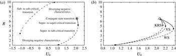
Figure 2(a) shows the full solution space for
 $R(U_{0})$
for the KRS model with
 $r=0.1$
and
 $s=1$
. However, not all possible solutions are physically relevant. Allowable solutions are determined, in part, by the long-wave phase speeds,
 $c_{\pm }$
, in dimensional variables (Baines Reference Baines1995),
 $$\begin{eqnarray}c_{\pm }=\frac{u_{1}d_{2}+u_{2}d_{1}}{D}\pm \left[g^{\prime }\frac{d_{1}d_{2}}{D}\left(1-\frac{(u_{1}-u_{2})^{2}}{g^{\prime }D}\right)\right]^{1/2}\end{eqnarray}$$
on either side of the jump. The sub- and super-criticality of the upstream and downstream regions are indicated in figure 2. Here
 $c_{-}<0$
(
 ${>}0$
) implies sub-criticality (super-criticality). If the negative characteristics upstream and downstream of the transition converge, a jump is expected to occur. If they diverge, an initially imposed jump will produce a rarefaction wave. Solutions with converging negative characteristics fall into one of three categories: super- to super-critical, super- to sub-critical or sub- to sub-critical. The behaviour of the positive characteristics does not affect the formation of a shock.
(a) Full solution space for the KRS theory with
 $r=0.1$
and
 $s=1$
. (b) Allowable solution space for KRS, WS and VS theories for
 $r=0.1$
and
 $s=1$
. Line type indicates behaviour of characteristics as marked in (a).

While the full solution space of the KRS theory is shown in figure 2(a), only a limited range of these solutions are physically allowable. To be structurally stable, solutions must have real
 $c_{\pm }$
and steady jump solutions require converging negative characteristics. Also, the total energy flux must decrease or be conserved across the jump so that
 $$\begin{eqnarray}\left[\int _{0}^{D}u\left(p+{\it\rho}\frac{u^{2}}{2}+{\it\rho}gz\right)\text{d}z\right]_{a}^{b}\leqslant ~0.\end{eqnarray}$$
Finally,
 $U_{0}$
must be positive to be consistent with the definition of upstream.
The allowable solution spaces of the KRS, VS and WS theories that satisfy these criteria are shown in figure 2(b) for
 $r=0.1$
and
 $s=1$
. The allowable solutions include super- to sub-critical jumps and super- to super-critical jumps. A special solution, called the conjugate-state solution (Lamb Reference Lamb2000), is also indicated in figure 2(b). This solution conserves energy in both layers, and the interfacial wave speeds upstream and downstream of the jump are the same. The KRS, WS and VS models all converge to the conjugate-state solution. The downstream height
 $R$
of this special solution is equal to the maximum internal solitary wave amplitude in the given upstream flow (Benjamin Reference Benjamin1968; Stastna & Lamb Reference Stastna and Lamb2002). The maximum possible
 $U_{0}$
occurs at the transition from sub- to super-critical and super- to super-critical jumps. This leads to a range of
 $U_{0}$
with two possible solutions for
 $R$
.
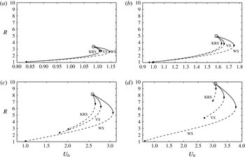
The allowable solutions for
 $r=0.1$
with
 $s=-1$
, 0, 2 and 3 are shown in figure 3(a–d), respectively. For all theories with the same
 $s$
, the maximum possible
 $R$
, which is the conjugate-state solution, is the same. The minimum value of
 $R$
(
 ${>}1$
) also increases for the KRS model, and to a lesser degree for the VS model as
 $s$
increases. The persistence of small jumps for large
 $s$
in the WS solutions is consistent with Klemp et al. (Reference Klemp, Rotunno and Skamarock1997), who suggest that small jumps with larger shear are better predicted by WS theory, while large jumps with small shear agree more with KRS theory. When the shear increases enough, the models no longer give any allowable solutions. For
 $r=0.1$
, the allowable solution space of the KRS theory extends to
 $s=3.15$
, and for the VS and WS theories, it ends at
 $s=3.18$
. For
 $r=0.2$
, the allowable solution space extends to
 $s=2.23$
for all three theories. As shear increases, the KRS theory solution space recedes toward the conjugate-state solution and then disappears. The two solutions for
 $R=1$
in the full solution space, shown in figure 2(a), approach each other as shear increases. They coalesce and then move off the
 $R=1$
line, at that point the WS and VS theories no longer produce allowable solutions. However, the WS and VS theories maintain a solution curve until this shear value, rather than receding to a single solution as the KRS theory does. As
 $s$
approaches the upper limit for solutions, the maximum allowable jump height (the conjugate-state solution) approaches
 $r^{-1}$
.
(a) Allowable solution space for KRS, WS and VS theories for
 $r=0.1$
and
 $s=-1$
. (b) Allowable solution space for KRS, WS and VS theories for
 $r=0.1$
and
 $s=0$
. (c) Allowable solution space for
 $r=0.1$
and
 $s=2$
, and (d) allowable solution space for
 $r=0.1$
and
 $s=3$
. Line type indicates behaviour of characteristics as marked in figure 2(a).

When
 $s>0$
, there are solutions for
 $R<1$
(i.e. drops in the lower-layer height across the jump). However, these solutions occur for
 $U_{0}<s$
and are thus exchange flows. Furthermore they have diverging negative characteristics, and would result in a rarefaction wave rather than a hydraulic jump and thus violate our allowable solution criteria.
Without upstream shear, the KRS theory, which conserves energy in the lower (expanding) layer, is more applicable than the WS theory, according to Klemp et al. (Reference Klemp, Rotunno and Skamarock1997), although the VS theory, which also dissipates most of the energy in the upper layer, agrees well with simulations in the same parameter range in which the KRS theory works well. Focusing on flows without upstream shear, Borden et al. (Reference Borden, Meiburg and Constantinescu2012) recently modified the KRS theory to allow a finite thickness vertical shear layer downstream of the jump that permits momentum and energy transfer from the faster (upper) to the slower (lower) layer. Instead of conserving energy as the KRS theory does, the Borden et al. (Reference Borden, Meiburg and Constantinescu2012) modification allows an energy increase in the lower layer. This idea has been extended to flows with upstream shear, although the results are very similar to the KRS theory for large jumps with small upstream shear and to the WS theory for small jumps with large shear, so the remainder of the article focuses on the KRS, WS and VS theories.
3. Numerical modelling
The theories discussed in § 2 apply to two-layer flows and do not account for the flow within the transition region of the jump that involves non-hydrostatic effects and turbulent mixing. Numerical simulations are thus used to investigate these effects and compared to the two-layer theories to determine which, if any, predicts the behaviour of the more realistic numerical simulations.
The numerical simulations use the non-hydrostatic, adaptive-mesh model IAMR (Almgren et al. Reference Almgren, Bell, Colella, Howell and Welcome1998). The model solves the incompressible Navier–Stokes equations,
 $$\begin{eqnarray}\left.\begin{array}{@{}c@{}}\displaystyle \frac{\partial \boldsymbol{u}}{\partial t}+\boldsymbol{u}\boldsymbol{\cdot }\boldsymbol{{\rm\nabla}}\boldsymbol{u}=-\frac{1}{{\it\rho}}\boldsymbol{{\rm\nabla}}p+{\it\nu}{\rm\nabla}^{2}\boldsymbol{u}-g\hat{k},\\ \displaystyle \frac{\partial {\it\rho}}{\partial t}+\boldsymbol{u}\boldsymbol{\cdot }\boldsymbol{{\rm\nabla}}{\it\rho}={\it\kappa}{\rm\nabla}^{2}{\it\rho},\\ \boldsymbol{{\rm\nabla}}\boldsymbol{\cdot }\boldsymbol{u}=0.\end{array}\right\}\end{eqnarray}$$
Here
 $\boldsymbol{u}=(u,v,w)$
, with
 $u$
the along channel,
 $v$
the transverse (for 3-D simulations only) and
 $w$
the vertical velocities. The density is
 ${\it\rho}$
,
 $p$
is the pressure,
 ${\it\nu}$
is the kinematic viscosity,
 ${\it\kappa}$
is the density diffusivity,
 $g$
is the magnitude of gravitational acceleration and
 $\hat{k}$
is the unit vector in the vertical direction. The model employs an adaptive Cartesian grid and a time centred, second-order projection method with a Godunov scheme for the advective terms. The model runs presented here are done in a non-Boussinesq mode required for the open boundaries (see below), although all simulations are essentially Boussinesq with
 ${\rm\Delta}{\it\rho}/{\it\rho}_{1}=0.02$
.
IAMR falls into a class of models that have been termed implicit large-eddy simulation (ILES) models. Because of the non-oscillatory, finite-volume Gudonov treatment of the nonlinear advection terms, the sub-grid stress is in the same form as a viscous stress tensor (Margolin, Rider & Grinstein Reference Margolin, Rider and Grinstein2006; Grinstein, Margolin & Rider Reference Grinstein, Margolin and Rider2007; Aspden et al. Reference Aspden, Nikiforakis, Dalziel and Bell2008). The numerical error acts as a turbulence scheme, dissipating energy at the grid scale, while conserving mass and momentum, and accurately capturing the energy cascade from resolved scales to the dissipation range at the grid scale. ILES models have been shown to give solutions that compare very well with DNS and traditional LES models for unstratified turbulent flows (Margolin et al. Reference Margolin, Rider and Grinstein2006; Grinstein et al. Reference Grinstein, Margolin and Rider2007; Aspden et al. Reference Aspden, Nikiforakis, Dalziel and Bell2008; Zhou et al. Reference Zhou, Grinstein, Wachtor and Haines2014), passive-scalar mixing (Hickel, Adams & Mansour Reference Hickel, Adams and Mansour2007) and stratified flows (Waite & Smolarkiewicz Reference Waite and Smolarkiewicz2008; Remmler & Hickel Reference Remmler and Hickel2012). White & Helfrich (Reference White and Helfrich2013) found very good agreement of kinetic energy dissipation and irreversible mixing between DNS calculations and ILES solutions with IAMR for intense stratified turbulence in a horizontal shear layer subject to gravitational tilting. These studies support the use of the ILES method for modelling energetic stratified flows such the hydraulic jumps considered here.
The numerical model results are non-dimensionalized in the same way as the two-layer theories and a scaled density
 $$\begin{eqnarray}b=\frac{{\it\rho}-{\it\rho}_{2}}{{\it\rho}_{1}-{\it\rho}_{2}}\end{eqnarray}$$
is introduced. Most of the simulations are done in two dimensions with a domain of
 $x\in [0,L_{x}]$
and
 $z\in [0,L_{z}]$
where
 $L_{z}=r^{-1}$
and
 $L_{x}\gtrsim 10r^{-1}$
. Simulations are initialized with an imposed smooth transition region that adjusts to form a hydraulic jump. In the initial conditions, all of the non-dimensional parameters are set and the transition region, or jump, is stationary. The initial velocity and density fields, in the non-dimensional variables introduced above, vary smoothly in the vertical through a hyperbolic tangent profile with height scale
 ${\it\lambda}^{-1}$
according to
 $$\begin{eqnarray}u(x,z,t=0)=\frac{\hat{U} _{0}}{d_{1}(x)}+\frac{{\it\delta}u(x)}{2}(1-\tanh [{\it\lambda}(z-d_{1}(x))]),\end{eqnarray}$$
and
 $$\begin{eqnarray}b(x,z,t=0)={\textstyle \frac{1}{2}}(1-\tanh [{\it\lambda}(z-d_{1}(x))]).\end{eqnarray}$$
The interface position,
 $d_{1}(x)$
, is given by
 $$\begin{eqnarray}d_{1}(x)=1+\frac{\hat{R}-1}{2}\left(1+\tanh \left[\frac{(x-x_{0})}{L}\right]\right),\end{eqnarray}$$
and the velocity jump between the layers,
 $$\begin{eqnarray}{\it\delta}u(x)=\frac{\hat{U} _{0}}{d_{1}(x)}-\frac{(r^{-1}-1)(\hat{U} _{0}-s)}{r^{-1}-d_{1}(x)}.\end{eqnarray}$$
Here
 $x_{0}$
is the initial location of the jump and
 $L$
is the horizontal length scale of the transition.
 $\hat{R}$
is the initial height of the transition and
 $\hat{U} _{0}$
is the initial upstream lower-layer velocity that are found from a two-layer model solution. The initial vertical velocity is zero at the top and bottom of the domain and defined so that the flow satisfies the continuity equation,
 $$\begin{eqnarray}w(x,z,t=0)=-\int _{0}^{z}\frac{\partial u(x,z^{\ast },t=0)}{\partial x}\,\text{d}z^{\ast }.\end{eqnarray}$$
The upstream inlet conditions are given by (3.3) and (3.4) evaluated at
 $x=0$
. An open boundary condition at
 $x=L_{x}$
, where the density and velocities satisfy Neumann conditions and the pressure is hydrostatic, allows the flow to leave the domain. Free-slip conditions are imposed at the top and bottom boundaries. Thus upstream of the transition,
 $d_{1}=1$
and
 ${\it\delta}u=s$
, while far downstream,
 $d_{1}=\hat{R}$
and
 ${\it\delta}u$
is given by (3.6), which satisfies the two-layer continuity condition. Initial values for
 $r$
,
 $s$
,
 $\hat{U} _{0}$
and
 $\hat{R}$
are chosen based on the allowable solution space from the two-layer theories.
 $\hat{U} _{0}$
values from both the KRS and WS theories were tested for a range of
 $\hat{R}$
values. During a simulation the jump front will usually translate at a small, constant speed and the jump height
 $\hat{R}$
may also adjust. For comparison with the theories the simulations are shifted into the frame moving with the jump.
 $\hat{U} _{0}$
is adjusted by the speed of the jump to give
 $\overline{U}_{0}=\hat{U} _{0}-\overline{U}_{b}$
, where
 $\overline{U}_{b}$
is the time-averaged speed of the jump. Therefore, many of the results presented here were initiated with
 $\hat{U} _{0}$
values chosen so that the speed of the jump front would be small and the jump would remain in the domain, away from boundaries, for as long as possible. This was achieved by setting
 $\hat{U} _{0}$
between the KRS and VS theories for large
 $\hat{R}$
, and larger than the WS theory for small
 $\hat{R}$
.
In the simulation results that will be shown,
 ${\it\lambda}=9$
,
 $L=3.75$
,
 $x_{0}=25$
,
 ${\it\rho}_{1}=1+{\rm\Delta}{\it\rho}=1.02$
and
 ${\it\rho}_{2}=1$
. The initial interface between the upper and lower layer, parameterized by
 ${\it\lambda}$
, is very thin, approximating a two-layer flow.
An isotropic grid with spatial, but temporally stationary, refinement is employed. The low resolution regions are concentrated near the upper boundary and just upstream of the outlet. The latter helps with the open boundary implementation. However, the active jump region is always contained within the finest grid that has an effective resolution of 256 cells in the vertical. The time step varies such that the maximum CFL number
 ${\leqslant}0.75$
. Several tests have been run to ensure that the domain lengths employed are sufficient to prevent the open downstream boundary condition from significantly influencing the results. In most simulations, there is no explicit viscosity or diffusivity (
 ${\it\nu}={\it\kappa}=0$
), so that the effects of any turbulence are handled through ILES. Some simulations with explicit viscosity and diffusivity are conducted, and are discussed further in § 3.2.
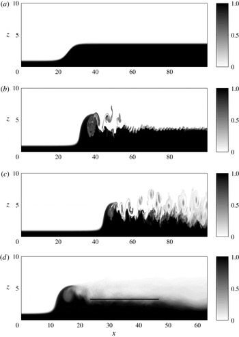
As an example of the numerical modelling approach, plots of the density field
 $b$
from a 2-D calculation initiated for
 $r=0.1$
,
 $s=1$
, and with
 $\hat{U} _{0}=2.1$
and
 $\hat{R}=3.7$
model are shown at
 $t=0$
, 62.6 and 157 in figure 4(a–c). The initial transition steepens and small-scale shear instabilities quickly form on the downstream interface (
 $t=62.6$
). The upstream flow has a minimum Richardson number of
 $Ri_{min}=2/({\it\lambda}{\it\delta}u^{2})=0.22$
, and the downstream section, where
 ${\it\delta}u=-1.0$
initially, also has
 $Ri_{min}=0.22$
, consistent with the development of downstream shear instability. The upstream section remains smooth because no disturbances are added to the inlet flow and the Kelvin–Helmholtz instability for the weakly unstable inflow has a relatively slow growth rate. The downstream section is disturbed by the steepening bore front, and the downstream wave and flow velocities are slower, allowing disturbances to grow before propagating out of the domain. Coherent vortices are subsequently shed in the lee of the bore front and are swept downstream, dominating the downstream interface so that the small-scale shear instabilities are no longer apparent (
 $t=157$
). The bore front moves slowly downstream at a constant speed. The time-averaged density field of the fully developed jump in this steadily moving reference frame of the bore front is shown in figure 4(d), averaged from
 $t=157{-}189$
. Note that this average plot has the bore front arbitrarily shifted to
 $x\approx 10$
. For these parameter values, the quasi-steady jump has a smooth front followed by a turbulent interfacial region. The details of the jump structure are discussed more in the next section.
Example 2-D numerical solution for an initial bore with
 $r=0.1$
,
 $s=1$
,
 $\hat{U} _{0}=2.1$
and
 $\hat{R}=3.7$
. The panels show the instantaneous density field
 $b$
at (a)
 $t=0$
, (b)
 $t=62.6$
, (c) and
 $t=157$
. The average density field of the fully developed jump, in a frame of reference moving with the bore, is shown in (d). The fully developed jump has
 $r=0.1$
,
 $s=1$
,
 $\overline{U}_{0}=1.99$
and
 $\overline{R}=3.28$
.

To compare the numerical model results to the two-layer theories, the four non-dimensional parameters of the fully adjusted flow,
 $r$
,
 $s$
,
 $\overline{U}_{0}$
and
 $\overline{R}$
, are needed. The initial upstream conditions define
 $r$
and
 $s$
, which do not change as the flow develops. To determine
 $\overline{R}$
, the interface is first located as follows. At every
 $x$
, the interface is defined so that the vertical integral of the density profile from the simulation is equal to the vertical integral of a two-layer density profile with interface height
 $\tilde{R}(x)$
,
 $$\begin{eqnarray}\tilde{R}(x)=\int _{0}^{r^{-1}}b(x,z)\,\text{d}z.\end{eqnarray}$$
The interface depth
 $\tilde{R}(x)$
downstream of the jump is then averaged over a region where the flow is approximately horizontally uniform to give a final value,
 $\overline{R}$
. This region excludes the jump front and the part of the domain just upstream of the outlet. The horizontal line in the time-averaged field in figure 4(d) indicates the averaging interval. The bore front, identified as the along channel location where the interface height reaches
 $\tilde{R}=({\it\epsilon}R-1)/4+1$
, is tracked. For jumps with a smooth front,
 ${\it\epsilon}=1.2$
, while
 ${\it\epsilon}=1.08$
is used for jumps with a turbulent front. The horizontal velocities are then adjusted into a frame of reference moving with the bore, giving
 $\overline{U}_{0}$
. The simulations are analysed over a time during which the speed of the bore front is approximately steady, resulting in less than 2 % variation in
 $U_{0}$
for the smooth-front jump shown in figure 4. Jumps with a turbulent front have more variation in the speed of the front (approximately 10 % variation in
 $U_{0}$
), although the speed oscillates about a constant value and does not exhibit a trend.
This procedure allows each simulation to be directly compared to the two-layer theories. For the solution shown in figure 4, this gives
 $\overline{U}_{0}=1.99$
and
 $\overline{R}=3.28$
. Recall that the initial conditions of the simulation were
 $\hat{U} _{0}=2.1$
and
 $\hat{R}=3.7$
, so that the numerical solution evolved to a slightly slower and smaller jump than was used for the initial conditions.
A large number of 2-D simulations, and a few 3-D runs (discussed separately in § 5), have been carried out for
 $r=0.1$
and
 $s=0{-}2$
to explore the jump structure and the mean downstream density and velocity fields. A smaller set of simulations with
 $r=0.2$
have also been conducted, but the calculations for
 $r=0.1$
are illustrative of results and are the focus of the effort.
3.1. Solution types
For flows with positive shear (
 $s>0$
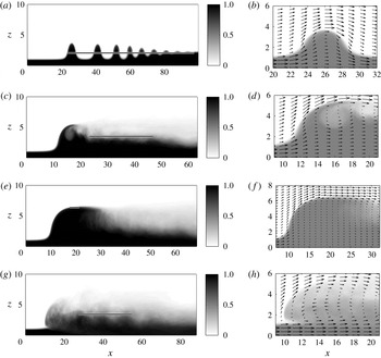
), four distinct, qualitatively different jump types were found in the numerical simulations. They are undular bores, smooth-front turbulent jumps, fully-turbulent jumps and conjugate-state transitions. Undular bores (UB) consist of a train of solitary-like waves, with the lower-layer depth increasing slightly after each wave up to the uniform downstream level, as shown in figure 5(a). The corresponding velocity field, shown in figure 5(b), is approximately parallel to isopycnals. There is very little mixing. Consequently, energy loss across the front is due to wave radiation as the train of solitary-like waves spreads with time.
Turbulent jumps may be smooth-front turbulent jumps (SFTJ), with a smooth wave-like front, as shown in figure 5(c,d). In these jumps, the velocity along the bore front is in the upward and downstream direction, with a small counter-clockwise recirculation region (vorticity the same sign as the upstream shear layer) slightly downstream of the front. Alternatively, turbulent jumps may be fully turbulent jumps (FTJ) with an overturning leading edge, as shown in figure 5(g,h). The velocity field figures show that the mean jump consists of two counter-rotating recirculation regions. In both SFTJ and FTJ cases, the interface region downstream of the jump is turbulent with substantial vertical mixing of density and momentum.
The fourth type are conjugate-state (CS) jumps. These are smooth wave-like transitions, which are, in theory, energy conserving. This type of jump is very close to the theoretical conjugate-state transition discussed in § 2.1, and corresponds to the maximum allowable height of the ‘table-top’ internal solitary wave (Grimshaw et al.
Reference Grimshaw, Pelinovsky, Talipova and Kurkin2004). Numerical simulations of this type of transition exhibit a steady form with very little mixing immediately downstream of the front, which is consistent with energy conservation. For flows without upstream shear, the layer depths downstream of the jump have equal thickness. As shear is increased, the downstream lower-layer depth exceeds half of the total depth (Stastna & Lamb Reference Stastna and Lamb2002). An example of a conjugate-state solution with some upstream shear is shown in figure 5(e,f). Within and immediately downstream of the front, the velocity is approximately along isopycnals, resulting in very little mixing, consistent with the theoretical conjugate-state solution. However, downstream shear instabilities do eventually emerge. These instabilities appear to trip a secondary hydraulic drop from the super-critical flow immediately downstream of the front to a sub-critical state at
 $x\approx 30$
. This super- to sub-critical drop is considered to be a separate feature from the upstream CS transition and may be linked to the presence of an imperfect outflow boundary.
The instantaneous density field,
 $b$
, is shown at a non-dimensional time of 157 for (a) an undular bore with
 $r=0.1$
,
 $s=1$
,
 $\overline{R}=2.00$
and
 $\overline{U}_{0}=1.75$
. Time-averaged density fields are shown for (c) a smooth-front turbulent jump with
 $r=0.1$
,
 $s=1$
,
 $\overline{R}=3.28$
and
 $\overline{U}_{0}=1.99$
, (e) a conjugate-state transition with
 $r=0.1$
,
 $s=1$
,
 $\overline{R}=6.42$
and
 $\overline{U}_{0}=2.08$
, and (f) a fully turbulent jump with
 $r=0.1$
,
 $s=1.5$
,
 $\overline{R}=3.12$
and
 $\overline{U}_{0}=2.59$
. The density field and velocity vectors are shown in the region of the jump in (b,d,f,h). Note that the density field shown with the velocity vectors uses lighter shades so that the vectors are visible.

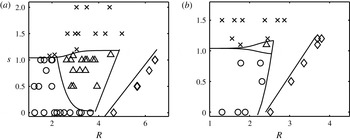
The type of jump that occurs depends on the final jump height
 $\overline{R}$
and the upstream shear
 $s$
, for a given
 $r$
. Figure 6 shows jump-type regime diagrams for
 $r=0.1$
and
 $r=0.2$
. Small jumps or jumps with small
 $s$
are undular bores. Large jumps with
 $s\leqslant 1$
near the theoretical, two-layer CS solution are conjugate-state jumps. Increasing
 $s$
for moderate
 $\overline{R}$
gives smooth-front turbulent jumps, and further increases in
 $s$
lead to fully-turbulent jumps at all jump heights. For larger
 $s$
, the conjugate-state solutions are lost due to intense interfacial instabilities that develop. The distribution of jump types changes with
 $r$
, although the same jump types and the trends described above are maintained.
The solution type depends on the jump height
 $\overline{R}$
and the upstream shear
 $s$
. Each point represents a numerical simulation of a given shear and jump height.
 $\times =$
fully turbulent jump, ○
 $=$
undular bore, ▵
 $=$
smooth-front turbulent jump and ♢
 $=$
conjugate state. (a)
 $r=0.1$
; (b)
 $r=0.2$
.

An interesting behaviour is found for moderate shear values near
 $s=1.1$
. Smaller jumps with
 $\overline{R}<2.5$
are fully turbulent (FTJ), whereas larger jumps are smooth-front turbulent jumps (SFTJ). This is counterintuitive because increased shear and jump height tend to increase instability and turbulence. However, as will be discussed in § 3.3, this unexpected behaviour can be linked to the properties of nonlinear waves in the upstream wave guide.
Finally, for a fixed
 $s\leqslant 1$
, there is a gap between the largest SFTJ or UB and the CS solutions. This gap corresponds to the region of super- to super-critical jumps in the two-layer models shown in figure 2. Although these solutions are physically allowable, a numerical simulation initiated in this region will either evolve to a solution near the conjugate state if the initial condition is close enough, or to a jump in the super- to sub-critical region. This gap is further illustrated in the next section where the numerical solutions are compared to the two-layer models.
This work focuses on flows with positive shear (
 $s>0$
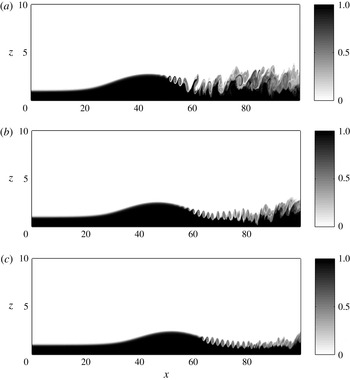
), which have a faster moving lower layer relative to the jump, as this is the type of flow that is generated by topography in locations such as Hood Canal and Knight Inlet. However, as seen in figure 3, allowable solutions exist for
 $s<0$
. Because the sign of the upstream vorticity is positive (opposite sign from
 $s$
), these solutions are structurally different from those that develop when
 $s>0$
. An example is shown for
 $s=-1$
in figure 7. Jumps with different initial values for
 $R$
and
 $U_{0}$
develop similarly. When
 $s<0$
, interfacial instabilities are enhanced because the jump increases the downstream interfacial shear. These instabilities are generally swept downstream, leaving a smooth, solitary wave, or undular bore, type of transition. Overturning at the leading edge of the jump is inhibited by the positive ambient vorticity. Furthermore, jumps with
 $s<0$
only have allowable solutions for small
 $R$
, which, along with the direction of the vorticity, helps to explain why they are similar to the undular bores found for
 $s\geqslant 0$
(cf. figure 6).
The instantaneous density field,
 $b$
, is shown at non-dimensional times of
 $t=125$
(a), 219 (b), and 313 (c) for initial conditions of
 $s=-1$
,
 $\hat{R}=3.4$
, and
 $\hat{U} _{0}=1.08$
.

3.2. Numerical simulations compared to layer theories
The two-layer theories might be used to predict the approximate height of a stationary (
 $c=0$
) hydraulic jump, given the upstream layer thicknesses and velocities. Klemp et al. (Reference Klemp, Rotunno and Skamarock1997) claim that large jumps without shear should be best predicted by the KRS theory, especially when
 $r\ll 1$
. However, they find that in jumps with upstream shear, the upstream vorticity changes the structure of the jump and the WS theory may be more accurate (Klemp et al.
Reference Klemp, Rotunno and Skamarock1997). The VS theory, which replaces specification of the distribution of dissipation with a vorticity conservation condition, gives predictions between the KRS and WS theories. White & Helfrich (Reference White and Helfrich2014) recently developed a theory for flows with continuous stratification without upstream shear, which allows the form of the dissipation to be specified. In the two-layer limit, the form of the dissipation can reduce their theory to any of the three two-layer theories specified above. However White & Helfrich (Reference White and Helfrich2014) find that the form that maximizes the total dissipation more accurately matches their numerical simulations. This form transfers energy from the upper to the lower layer, an idea that was also used by Borden et al. (Reference Borden, Meiburg and Constantinescu2012), who modified the KRS model to transfer energy from the upper to the lower layer.
Simulation results for
 $\overline{R}$
and
 $\overline{U}_{0}$
are compared to the KRS, VS and WS theories with
 $r=0.1$
and
 $s=1$
and
 $s=1.5$
in figure 8(a,b), respectively. The qualitative jump type is also indicated. For moderate shear of
 $s=1$
(figure 8
a), small jumps (
 $\overline{R}\lesssim 2$
) agree best with the WS theory, while for larger jumps (
 $\overline{R}\gtrsim 3$
), the simulations are in better agreement with the KRS theory. The tendency for smaller jumps (and with smaller
 $\overline{U}_{0}$
) to agree with the WS model and larger jumps with the KRS model is in broad agreement with the hypothesis of Klemp et al. (Reference Klemp, Rotunno and Skamarock1997). Also note that the jump type is an undular bore for
 $\overline{R}\lesssim 2$
and a smooth-front turbulent jump for larger amplitudes, with the exception of a conjugate-state jump for
 $\overline{R}\approx 6.4$
. Jumps initiated in the super- to super-critical region of
 $4\lesssim \hat{R}\lesssim 6.4$
develop into either a conjugate-state transition if
 $\hat{R}$
is large enough (
 $\hat{R}\gtrsim 6$
), or retreat to a smaller super- to sub-critical transition if
 $\hat{R}$
is smaller. This leaves a gap in the solution space where theoretical super- to super-critical jumps are possible, but numerical solutions do not exist. A possible explanation for this behaviour lies in the energy loss associated with each of these branches. For the same
 $U_{0}$
, the downstream sub-critical theoretical solution with a smaller
 $R$
has more dissipation and less downstream vertical shear than the larger, super-critical solution. This suggests that when two solutions are theoretically possible, the solution that dissipates more energy through the jump is selected.
(a) Theoretical solution space and numerical simulation results for
 $r=0.1$
and
 $s=1$
. ▫
 $=$
conjugate-state transition, ○
 $=$
undular bore, ▵
 $=$
smooth-front turbulent jump. ●
 $=$
3-D undular bore, ▴
 $=$
3-D smooth-front turbulent jump,

 $=$
2-D high-resolution smooth-front turbulent jump with
 $Re=1250$
and
 $Sc=1$
. (b) Theoretical solution space and numerical simulation results for
 $r=0.1$
and
 $s=1.5$
, ♢
 $=$
2-D fully-turbulent jump, ♦
 $=$
3-D fully-turbulent jump,

 $=$
2-D high-resolution fully-turbulent jump with
 $Re=1250$
and
 $Sc=1$
. Error bars show one standard deviation of
 $\tilde{R}(x)$
.

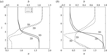
Along channel velocity and density profiles downstream of the jump, averaged in space and time. (a) Smooth-front turbulent jump with
 $r=0.1$
,
 $s=1$
,
 $\overline{U}_{0}=1.99$
,
 $\overline{R}=3.28$
averaged from
 $t=157{-}189$
and
 $x=23{-}47$
. (b) Fully-turbulent jump with
 $r=0.1$
,
 $s=1.5$
,
 $\overline{U}_{0}=2.59$
,
 $\overline{R}=3.12$
averaged from
 $t=157{-}189$
and
 $x=27{-}55$
.

Simulations with higher upstream shear,
 $s=1.5$
, shown in figure 8(b), generally fall between the WS and VS predictions. The larger jumps do tend to lie closer to the VS curve, but there is substantial scatter in
 $\overline{R}$
for the similar values of
 $\overline{U}_{0}$
. All of these jumps in figure 8(b) are the fully-turbulent type, which may explain the increased scatter.
Although these simulations give some support to transitions between the two-layer WS and KRS models suggested by Klemp et al. (Reference Klemp, Rotunno and Skamarock1997), there is significant scatter in the numerical data, and none of the two-layer theories performs particularly well for the parameter values examined. This is perhaps not too surprising since the two-layer theories neglect flow features such as continuous velocity and density profiles, as well as the dynamics and structure within the jump. Velocity and density profiles, averaged in time and in space downstream of the jump, are shown in figure 9(a) for a smooth-front turbulent jump (for
 $t=157{-}189$
and
 $x=23{-}47$
) and in figure 9(b) for a fully-turbulent jump (for
 $t=157{-}189$
and
 $x=27{-}55$
). The time-averaged density fields are shown in figure 5(c,g), respectively. While the downstream density profiles have monotonic variation with height and are reasonably close to two-layered, the velocity profiles exhibit a velocity minimum between the layers. It is particularly pronounced for the higher shear,
 $s=1.5$
, fully-turbulent jump in figure 9(b). The velocity minimum occurs in the lee of the bore head, where the streamlines slowly expand to fill the space behind the bore, and the influence of the jump is felt well downstream of the front.
It is also interesting to note that the strongest density gradient is not coincident with the velocity shear layer. For the smooth-front turbulent jump in figure 9(a), the velocity shear layer extends higher than the density gradient, and for the FTJ, the shear layer extends above and below the density-gradient layer. This shear in the velocity profile is generated by baroclinic torque in the turbulent jump-head region. These velocity and density profiles are very different from the idealized two-layer theories, and even from the Borden et al. (Reference Borden, Meiburg and Constantinescu2012) theory that assumes coincident linear mixing layers downstream of the jumps.
The theoretical models assume no fluid exchange between the layers, i.e. no entrainment. The numerical results show strong vertical mixing and departures from the two-layer assumptions that suggest when viewed in a two-layer limit, entrainment between the layers may occur. This as been assessed from the change in mean lower-layer volume flux across the jump
 $$\begin{eqnarray}{\rm\Delta}\overline{q}_{1}=\left[\int _{0}^{\overline{R}}\overline{u}(z)\,\text{d}z\right]_{a}^{b}.\end{eqnarray}$$
Over the range of parameters explored the entrainment,
 ${\rm\Delta}\overline{q}_{1}/\overline{q}_{1a}$
, into the lower layer is at most 10 %, and generally less than 5 %. As discussed in § 6, while entrainment can be incorporated into two-layer jump models, it does not seem to be critical in the parameter range considered here.
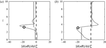
The change in energy along streamlines between the downstream averaged state and the upstream state,
 $$\begin{eqnarray}\left[\frac{\text{d}(\overline{u}\overline{B})}{\text{d}{\it\psi}}\right]_{a}^{b},\end{eqnarray}$$
is shown in figure 10(a,b) for the smooth-front turbulent jump and the fully-turbulent jump in figure 9(a,b). Here,
 $B$
is the Bernoulli function and
 $u$
is the horizontal velocity of the time-averaged fields. The derivative with respect to the streamlines,
 ${\it\psi}$
, accounts for the spreading of streamlines through the jump, giving a measure of how the distribution of the depth integrated energy flux changes across the jump. The circles indicate the height of the interface downstream of the jump,
 $\overline{R}$
, and the grey bars indicate the average energy flux change across the jump in each layer. In both the SFTJ and the FTJ, there is energy loss in the streamlines both above and below the downstream interface. In the smooth-front turbulent jump (figure 10
a), the streamlines near the interface lose the most energy, while there is a small gain in energy near the lower boundary. In contrast, the streamlines just above the interface of the fully-turbulent jump (figure 10
b) gain some energy, while the lower-layer loses energy. In both of these examples, the upper layer moves faster than the lower layer downstream of the jump (see figure 9), suggesting that the upper layer might transfer energy to the lower layer downstream of the jump. This transfer may be occurring in the smooth-front turbulent jump (figure 10
a) in which there is more energy lost in the upper layer than the lower layer, although it is not evident in the fully-turbulent jump (figure 10
b).
The energy loss in the smooth-front turbulent jump peaks in the middle of the velocity shear layer, where there is also a reduced vertical shear. This also corresponds with the upper part of the density gradient zone. In the fully-turbulent jump, there are two velocity shear zones, one through the lower part of the flow, with velocity decreasing with height, and another just above the two-layer interface, with velocity increasing with height, and they are separated by a thin layer of low shear. The largest dissipation occurs within this low-shear layer, which is also coincident with a region of high density gradient. In both cases, high dissipation coincides with a region of low vertical shear, indicating that the dissipation is tending to stabilize the flow. A similar calculation that includes the mean turbulent kinetic energy,
 $(\overline{u^{\prime 2}}+\overline{w^{\prime 2}})/2$
, in
 $\overline{B}$
gives nearly the same result, indicating that the turbulent contribution is negligible. This is expected because the turbulent quantities are much smaller than the means, particularly outside the jump transition region.
Energy flux difference along streamlines versus downstream height of streamline. (a) Smooth-front turbulent jump with
 $r=0.1$
,
 $s=1$
,
 $\overline{U}_{0}=1.99$
,
 $\overline{R}=3.28$
. (b) Fully-turbulent jump with
 $r=0.1$
,
 $s=1.5$
,
 $\overline{U}_{0}=2.59$
,
 $\overline{R}=3.12$
.
 $\overline{R}$
is indicated by ○. The average energy flux change in each layer is indicated by the light grey line through the layer.

Smooth-front turbulent jump heights with
 $r=0.1$
and
 $s=1$
are best described by the KRS and VS theories (figure 8
a). In the KRS model, all of the energy loss is in the upper layer, while in the VS theory, most of the energy loss occurs in the upper layer (approximately 80 % for the SFTJs shown here). The lower layer of the simulated flow loses less energy than the upper layer, consistent with the KRS and VS theories. The fully-turbulent jump is better described by the WS theory, which conserves energy in the upper layer, consistent with figure 10(b). However, in both cases the energy flux distributions of the simulations are much more complicated than the theories allow.
These results suggest, not surprisingly, that the energy changes across hydraulic jumps are not well described by two-layer theories that confine energy loss to a single layer or assume a simple distribution of energy loss and gain. White & Helfrich (Reference White and Helfrich2014) calculate theoretical energy-loss distributions for jumps with continuous density and velocity profiles and without upstream shear, and showed numerical simulation results for both an undular bore and a smooth-front turbulent jump. However, their resulting distributions are not consistent with those in figure 10, indicating that upstream shear influences the dissipation distribution. Their equivalent of the smooth-front turbulent jump (see their figure 5) exhibits significantly less mixing that is localized further downstream of the bore head than found here.
The vorticity budget can also be analysed to determine how well the simulations conserve vorticity across the jump, which is the basis of the VS theory (Borden & Meiburg Reference Borden and Meiburg2013b ). The vorticity budget for a stationary, Reynolds-averaged, Boussinesq, flow integrated over the area of the jump is (in scaled variables)
 $$\begin{eqnarray}\left[\int _{0}^{r^{-1}}\bar{u}\,\overline{{\it\omega}}_{2}\,\text{d}z\right]_{0}^{x}+\left[\int _{0}^{r^{-1}}\overline{u^{\prime }{\it\omega}_{2}^{\prime }}\,\text{d}z\right]_{0}^{x}-\int _{0}^{x}\int _{0}^{r^{-1}}\frac{\partial \bar{b}}{\partial x}\,\text{d}z\,\text{d}x=\oint _{C}{\it\nu}\boldsymbol{{\rm\nabla}}\overline{{\it\omega}}_{2}\boldsymbol{\cdot }\boldsymbol{n}\,\text{d}s,\end{eqnarray}$$
where
 ${\it\omega}_{2}=(\partial u/\partial z)-(\partial w/\partial x)$
is the vorticity in the
 $y$
-direction,
 $C$
is the contour bounding the control volume and
 $\boldsymbol{n}$
is the outward normal. The overbars indicate mean quantities and the primes denote turbulent departures from the time-mean flow. The first and second terms on the left are the divergence of mean and turbulent vorticity fluxes across the region, while the third term is the mean baroclinic production of vorticity within the region. The term on the right is the divergence of the viscous vorticity flux, which will generally be small for high Reynolds number flows. This equation includes the effect of turbulence that may result in vorticity fluxes across the mean streamlines and potentially disrupt the balance between the mean vorticity-flux divergence and baroclinic production (terms 1 and 3) assumed by Borden & Meiburg (Reference Borden and Meiburg2013b
). We note that these fluxes, if not explicitly included in the budget, could be interpreted as resulting from a turbulent viscosity that would appear in the viscous-flux term and are analogous to the production by gradients in (turbulent) dissipation across streamlines in White & Helfrich (Reference White and Helfrich2014).
The cumulative integral of each term are shown for a SFTJ in figure 11(a), and for a FTJ in figure 11(b). Also indicated in these figures is the downstream region used to find
 $\overline{R}$
, which is also used to determine the downstream-averaged values of the vorticity budget terms. The results show that the divergence of the vorticity flux is approximately balanced by the baroclinic production as assumed in the VS model. This is especially true for the SFTJ where the downstream-averaged turbulent fluxes are less than 0.4 % of the mean flux divergence. In the FTJ, the turbulent fluxes are slightly larger, about 6.2 %, of the mean flux divergence. In both examples the average residual is positive and comparable (2.2 % and 7.5 %, respectively) to the turbulent-flux divergence, indicating that the ILES (numerical) dissipation with the jump region is a small, but non-negligible, contribution to the vorticity budget. These two examples are typical of other runs and indicate that for the parameters considered the vorticity budget integrated over the jump region agrees reasonable well with the mean balance of Borden & Meiburg (Reference Borden and Meiburg2013b
).
Integrated vorticity budget terms for (a) smooth-front turbulent jump with
 $r=0.1$
,
 $s=1$
,
 $\overline{U}_{0}=1.99$
,
 $\overline{R}=3.28$
and (b) fully-turbulent jump with
 $r=0.1$
,
 $s=1.5$
,
 $\overline{U}_{0}=2.59$
,
 $\overline{R}=3.12$
.


All of the results presented so far relied entirely on the ILES properties of the numerical scheme to model the grid-scale dissipation and irreversible mixing. In order to assess the ILES calculations, several high-resolution runs with isotropic grids and 1024 cells in the vertical with finite
 $Re=(g^{\prime }d_{1a}^{3})^{3/2}{\it\nu}^{-1}=1250$
and
 $Sc={\it\nu}{\it\kappa}^{-1}=1$
were conducted. High-resolution runs for the SFTJ and FTJ cases of figure 5(c,g) are included in figure 8 and the results for
 $\overline{U}_{0}$
and
 $\overline{R}$
are within a few percent of the ILES values. In these finite-
 $Re$
runs, over 80 % of the total dissipation is resolved. Furthermore, for the SFTJ, the total dissipation in the high-resolution finite
 $Re$
simulation is very similar to that of the equivalent ILES run, and for the FTJ, the total dissipation of the high-resolution run is within a factor of 1.5 of ILES run. While the ILES is a compromise for computational efficiency, these comparisons support the approach as also found by White & Helfrich (Reference White and Helfrich2013). The simulation results for
 $Re=1250$
and
 $Re\rightarrow \infty$
agree, indicating that the results are not highly dependent on
 $Re$
in this parameter range. The value of
 $Sc=1$
was chosen because the applications of interest are highly turbulent, such that the turbulent Schmidt number would be approximately one.
3.3. Solitary wave solutions
Undular bore transitions have so far been classified as hydraulic jumps with the jump front identified as the front of the first wave. However, the simulations show that the wave packet slowly expands and the individual waves separate, acting more like a train of solitary waves than a sudden jump. The height of the leading wave might therefore be predicted from the relation between wave amplitude and speed for large-amplitude internal solitary waves obtained from the Dubreil–Jacotin–Long (DJL) model.
The DJL equation for steadily propagating internal solitary waves, in the Boussinesq limit and with an ambient shear flow, is (Stastna & Lamb Reference Stastna and Lamb2002)
 $$\begin{eqnarray}\displaystyle & \displaystyle {\rm\nabla}^{2}{\it\eta}+\frac{U^{\prime }(z-{\it\eta})}{c-U(z-{\it\eta})}[{\it\eta}_{x}^{2}+({\it\eta}_{z}-2){\it\eta}_{z}]+\frac{N^{2}(z-{\it\eta})}{(c-U(z-{\it\eta}))^{2}}{\it\eta}=0,\quad 0<z<D, & \displaystyle\end{eqnarray}$$
 $$\begin{eqnarray}\displaystyle & \displaystyle {\it\eta}(x,0)={\it\eta}(x,D)=\lim _{x\rightarrow \pm \infty }{\it\eta}(x,z)=0, & \displaystyle\end{eqnarray}$$
where
 ${\it\eta}(x-ct,z)$
is the isopycnal displacement,
 $N(z)$
is the background buoyancy frequency,
 $U(z)$
is the background shear profile and
 $c$
is the speed of the solitary wave. In the frame of reference moving with the leading wave,
 $U(z)$
is shifted so that
 $U(z)\rightarrow U(z)-c$
and
 $c\rightarrow 0$
. Simulation results for
 $\overline{U}_{0}$
can therefore be compared to DJL predictions using
 $U(0)-c$
. The DJL equation is solved numerically using the pseudo arc-length continuation method with Newton–Raphson iteration (Luzzatto-Fegiz & Helfrich Reference Luzzatto-Fegiz and Helfrich2014) with
 $U(z)$
and
 $N(z)$
from (3.3) and (3.4) evaluated upstream. The calculations are initialized with the Korteweg–de Vries solution for small-amplitude waves and then followed to give the solution curve for
 $c=c({\it\eta}_{max})$
, where
 ${\it\eta}_{max}$
is the maximum displacement. Each family of solutions ends at the limiting amplitude conjugate-state solution. To compare the lead wave of an undular bore to a DJL wave, the maximum height of the leading wave,
 $\tilde{R}_{max}$
, is obtained. The equivalent DJL wave amplitude is then
 $\tilde{R}_{max}-1$
.
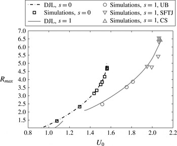
Results from the numerical simulations are compared to numerical solutions of the DJL equation for
 $s=0$
and
 $s=1$
with
 $r=0.1$
in figure 12. It should be noted that in the numerical simulations, the height of the interface downstream of the leading wave is higher than the interface upstream of the wave, whereas the DJL equation assumes symmetry in isopycnal displacement about the centre of the wave. Despite this difference, the DJL theory predicts the speed of the leading wave of an undular bore quite accurately. Furthermore, smooth-front turbulent jumps, which exhibit complete upstream–downstream asymmetry are also included in figure 12 and also show good agreement with the DJL relation
 $c=c(R_{max}-1)$
.
Interface height of leading wave (
 $R_{max}$
) versus lower-layer upstream speed (
 $U_{0}$
) relative to the leading wave. Numerical simulations are compared to convectively stable DJL predictions for
 $r=0.1$
. Note that the
 $s=1$
curve is discontinuous because convectively unstable solutions that occur for
 $1.4\lesssim R_{max}\lesssim 2.1$
, are not plotted.

DJL solutions for large shear values (
 $s\gtrsim 1$
) begin to exhibit convective instability for waves with moderate amplitudes (Stastna & Lamb Reference Stastna and Lamb2002; Choi Reference Choi2006). Convectively-unstable solutions develop trapped cores (Stastna & Lamb Reference Stastna and Lamb2002; Helfrich & White Reference Helfrich and White2010; Carr, King & Dritschel Reference Carr, King and Dritschel2012; Luzzatto-Fegiz & Helfrich Reference Luzzatto-Fegiz and Helfrich2014). The trapped-core solutions are distinguished by regions of closed streamlines with gravitationally unstable density distributions. With ambient shear the recirculation regions may be embedded within the body of the fluid near the interface (Choi Reference Choi2006). Streamlines in the recirculation zones do not extend to
 $|x|\rightarrow \infty$
, in violation of the assumptions used to derive the DJL equation. In figure 12, convectively-unstable DJL solutions develop for
 $s\gtrsim 1$
. Interestingly, the trapped-core solutions only appear in the limited amplitude range
 $1.4\lesssim R_{max}\lesssim 2.1$
for
 $s=1$
, and are excluded from the solution curve. Both smaller and larger wave solutions are convectively stable. The intermediate range of convectively-unstable solutions coincides with the appearance of fully-turbulent jumps, as shown in the regime diagram in figure 6(a) for
 $s=1.1$
. (Note that the regime diagram shows
 $\overline{R}$
, while
 $\tilde{R}_{max}$
must be considered in relation to the DJL predictions. Fully-turbulent jumps do not have a meaningful
 $\tilde{R}_{max}$
, and are therefore not included in figure 12.) These results emphasize the control that the upstream wave guide exerts on the bore and jump solutions, in agreement with the results of White & Helfrich (Reference White and Helfrich2014).
4. Mixing
An important consequence of internal hydraulic jumps is turbulent mixing, which dissipates energy and redistributes fluid properties. Mixing can be quantified through the time-averaged turbulent buoyancy flux,
 $\overline{w^{\prime }b^{\prime }}$
, and shear production,
 $\overline{u_{i}^{\prime }u_{j}^{\prime }}(\partial \overline{u}_{i}/\partial x_{j})$
. The primed quantities are deviations from the time-averaged mean of the fully-developed flow (in the frame moving with the bore front). The cumulative area integral of the buoyancy flux,
 $$\begin{eqnarray}\int _{0}^{x}\int _{0}^{D}\overline{w^{\prime }b^{\prime }}\,\text{d}z\,\text{d}x,\end{eqnarray}$$
and shear production,
 $$\begin{eqnarray}\int _{0}^{x}\int _{0}^{D}-\overline{u_{i}^{\prime }u_{j}^{\prime }}\frac{\partial \overline{u}_{i}}{\partial x_{j}}\,\text{d}z\,\text{d}x,\end{eqnarray}$$
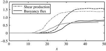
for the smooth-front turbulent jump shown in figure 4, with moderate shear of
 $s=1$
,
 $\overline{R}=3.28$
,
 $\overline{U}_{0}=1.99$
and
 $r=0.1$
, are shown in figure 13. The simulation is averaged over 151 time steps evenly spaced from
 $t=156$
to
 $t=250$
. The integral extends through the depth of the flow and from the inlet of the domain to a point
 $x$
downstream of the inlet. The figure shows that there is an area of intense mixing just downstream of the bore front at
 $x\approx 12$
, leading to a rapid increase in the cumulative buoyancy flux and shear production from
 $x\approx 15$
to
 $x\approx 25$
. Downstream, the cumulative buoyancy flux and shear production plateau. The average downstream cumulative buoyancy flux is a measure of the total mixing,
 $M$
, of the hydraulic jump. The horizontal extent of the averaging region is the same as used to obtain
 $\overline{R}$
and is indicated with a horizontal line in figure 13.
Cumulative integral of buoyancy flux and shear production along the domain for the pure ILES simulation with 256 grid points in the vertical for
 $r=0.1$
,
 $s=1$
,
 $\overline{U}_{0}=1.99$
and
 $\overline{R}=3.28$
(grey lines) and the fine grid (1024 grid points) simulation with
 $Re=1250$
and
 $Sc=1$
(black lines). The total mixing,
 $M$
, is indicated for the ILES case by the thick horizontal line.

Figure 13 also shows the cumulative buoyancy flux for a fine-grid simulation with explicit dissipation. The simulation has 1024 points in the vertical,
 $Re=1250$
, and
 $Sc=1$
. The cumulative buoyancy flux and shear production levels are very similar to the pure ILES case, indicating that the ILES approach of approximating turbulence is consistent with simulations in which nearly all of the dissipation is resolved. The region of mixing is shifted downstream in the simulation with a finite
 $Re$
as a result of a smoother density field in the bore head.
The total mixing,
 $M$
, versus jump height,
 $\overline{R}$
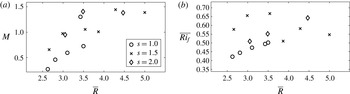
, is shown in figure 14(a) for 2-D simulations with several shear values. Shear and jump height both affect the magnitude of mixing. Larger jumps undergo more mixing, and FTJs experience more mixing than SFTJs. The conjugate-state jumps, however, are an exception to this trend. These large transitions undergo very little mixing (excluding the subsequent super- to subcritical drop), consistent with their energy-conserving properties.
The mixing efficiency,
 $$\begin{eqnarray}\overline{Ri_{f}}=\frac{1}{x_{2}-x_{1}}\int _{x_{1}}^{x_{2}}\left(\frac{\displaystyle \int _{0}^{x}\int _{0}^{D}\overline{w^{\prime }b^{\prime }}\,\text{d}z\,\text{d}x}{\displaystyle \int _{0}^{x}\int _{0}^{D}-\overline{u_{i}^{\prime }u_{j}^{\prime }}\frac{\partial \overline{u_{i}}}{\partial x_{j}}\,\text{d}z\,\text{d}x}\right)\text{d}x,\end{eqnarray}$$
shown in figure 14(b), does not exhibit an overall trend. The mixing efficiency is slightly higher for FTJs (
 $s=1.5$
and
 $s=2$
) than for SFTJs (
 $s=1$
), but does not increase with shear for a given jump structure. It increases slightly with increasing jump height for SFTJs, but this trend is weak and does not hold for FTJs.
(a)
 $M$
and (b)
 $\overline{Ri_{f}}$
versus
 $\overline{R}$
for
 $r=0.1$
and
 $s=1$
, 1.5 and 2 as indicated.

5. Three-dimensional simulations
Several three-dimensional simulations were carried out to determine whether the results are significantly altered. For all 3-D simulations, the initial setup is the same as the corresponding 2-D simulation, with the addition of periodic boundary conditions in the transverse,
 $y$
, direction. The width of the domain is one quarter of the height. The grid is isotropic with 256 grid points in the vertical and the simulations are run as pure ILES with zero explicit viscosity and diffusivity.
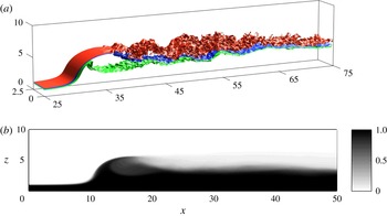
Instantaneous density surfaces of a 3-D simulation of a smooth-front turbulent jump with
 $r=0.1$
,
 $s=1$
,
 $\overline{U}_{0}=2.04$
and
 $\overline{R}=3.72$
(now also averaged in
 $y$
) are shown in figure 15(a) for
 $t=173$
, after the jump has fully adjusted. The initial conditions are equivalent to the 2-D case shown in figure 4. In the 3-D simulation, vortex rolls in the interface downstream of the jump are visible early in the flow development, but subsequently break down rapidly due to 3-D effects, whereas the 2-D simulations develop and maintain more coherent vortex rolls, as shown in figure 4(c). The jump is otherwise similar to the equivalent 2-D case, with
 $(\overline{U}_{0},\overline{R})=(1.99,3.28)$
in 2-D and (2.04, 3.72) in 3-D. The transverse and time-averaged density field for the 3-D simulation is shown in figure 15(b). It should be compared to the equivalent 2-D case in figure 4(d). Both the 2-D and 3-D simulations have been averaged in time from
 $t=157{-}188$
, with data saved at 51 evenly spaced time steps. The density field from the 3-D simulation is much smoother due to the breakdown of the vortex rolls. The downstream-averaged velocity and density profiles (figure 9
a) are also similar to the 2-D case, with a velocity minimum at the bottom of the shear layer and a thicker velocity-shear-layer than density-transition layer.
(a) Density surfaces of 3-D SFTJ. The density surfaces are
 $b=0.1$
(red), 0.5 (blue), 0.9 (green). Simulations parameters are
 $r=0.1$
,
 $s=1$
,
 $\overline{R}=3.72$
and
 $\overline{U}_{0}=2.04$
shown at
 $t=157$
. (b) Transverse and time-averaged density field.

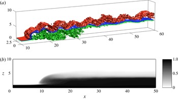
(a) Density surfaces of 3-D FTJ. The density surfaces are
 $b=0.1$
(red), 0.5 (blue), 0.9 (green). Simulations parameters are
 $r=0.1$
and
 $s=1.5$
,
 $\overline{R}=3.72$
and
 $\overline{U}_{0}=2.65$
.
 $t=172$
. (b) Transverse and time-averaged density field.

This 3-D smooth-front turbulent jump is included in the two-layer theory solution space in figure 8(a). A 3-D smooth-front turbulent jump with the same initial conditions and a domain width of half the total height (
 $r=0.1$
,
 $s=1$
,
 $\overline{R}=3.64$
and
 $\overline{U}_{0}=1.98$
), and a 3-D simulation result for an undular bore (
 $r=0.1$
,
 $s=1$
,
 $\overline{R}=1.96$
and
 $\overline{U}_{0}=1.76$
) are also shown in this figure. For all of these simulations, the 3-D results are close to their 2-D companions and within the scatter of the 2-D simulations.
Instantaneous density surfaces of a fully-turbulent hydraulic jump in 3-D with
 $r=0.1$
,
 $s=1.5$
,
 $\overline{U}_{0}=2.65$
and
 $\overline{R}=3.72$
are shown in figure 16(a). The transverse-averaged density field, averaged in time from
 $t=157{-}188$
using 51 time steps, is shown in figure 16(b), and should be compared to the equivalent 2-D case in figure 5(g) where
 $(\overline{U}_{0},\overline{R})=(2.59,3.12)$
. Downstream-averaged density and velocity fields, shown in figure 9(b), are similar to the equivalent 2-D case, with a velocity minimum at a height of
 $z\approx 3$
. The vertical density gradient at the interface between layers is sharper in the 3-D result and, while it is not obvious from figures 5(g) and 16(b), the horizontal density gradient across the bore front is sharper in the 2-D case, although the overall properties are otherwise similar. The 3-D simulation is compared with the two-layer theories in figure 8(b). While there are some qualitative differences between the 2-D and 3-D pair, the 3-D simulation falls within the scatter of the 2-D results.
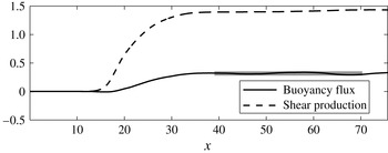
Cumulative integrals of buoyancy flux and shear production along the domain from the 3-D run with
 $r=0.1$
,
 $s=1$
,
 $\overline{U}_{0}=2.04$
and
 $\overline{R}=3.72$
. The total mixing
 $M$
, is indicated by the horizontal line.

Not surprisingly, vertical mixing in 3-D cases is quantitatively different from mixing in the equivalent 2-D flows due to vortex breakdown. Shear production of turbulent kinetic energy is consumed by this lateral mixing, reducing the turbulent kinetic energy available for buoyancy fluxes. The cumulative integrals of shear production and buoyancy flux are shown in figure 17 for the 3-D smooth-front turbulent jump with
 $r=0.1$
,
 $s=1$
,
 $\overline{U}_{0}=2.04$
and
 $\overline{R}=3.72$
. This should be compared to the equivalent 2-D case, shown in figure 13. The shear production is similar in 2-D and 3-D, but because of the energy lost to lateral mixing, the 3-D buoyancy flux is about half of the 2-D result, giving reduced mixing efficiency in 3-D.
In three dimensions the
 $y$
-vorticity budget (Boussinesq limit) will include vortex-stretching terms,
 ${\it\omega}_{i}\partial v/\partial x_{i}$
, that could disrupt the balance between mean vorticity-flux divergence and baroclinic production assumed in Borden & Meiburg (Reference Borden and Meiburg2013b
). However, analysis of the vorticity budgets of these 3-D runs gives results similar to the 2-D cases in figure 11. For the SFTJ the mean vorticity-flux divergence is 2.71 (per unit width) and the baroclinic production term is
 $-2.69$
. The sum of the mean and turbulent stretching terms is 0.02. The turbulent vorticity flux, 0.02, and residual, 0.04, are both similarly small. The stretching terms,
 $-0.01$
, are also insignificant in the FTJ where the primary balance is again between mean flux divergence, 2.96, and baroclinic production,
 $-2.68$
. The three-dimensional turbulent flux divergence is now positive, 0.44, and a slightly larger contributor to the overall balance than in 2-D. The residual, 0.74, is also larger, indicating that ILES (turbulent) dissipation is becoming important.
6. Conclusions
The full solution space of three basic two-layer theories for hydraulic jumps with upstream shear was explored. Allowable solutions were found in the super- to sub-critical and super- to super-critical branches of the solution space, including the maximal height, energy-conserving conjugate-state solution. For some upstream conditions, there are two theoretical downstream states, one of which is a super- to sub-critical transition, while the other is a super- to super-critical transition. When two theoretical solutions are possible, the numerical simulations fall along the super- to sub-critical branch unless they are initialized very close to the theoretical conjugate-state solution, in which case they result in conjugate-state jumps. The KRS and VS theories were in better agreement with the numerical results for large jumps with smaller shear, while the WS theory agreed better for smaller jumps and larger shear. This is consistent with the predictions of Klemp et al. (Reference Klemp, Rotunno and Skamarock1997). However, none of the basic two-layer theories were particularly accurate, and there was significant scatter in the numerical results. Furthermore, the downstream-averaged velocity and density profiles of the numerical simulations were significantly different from the strictly two-layer structure assumed in the theories, and also the linear shear-layer modification proposed by Borden et al. (Reference Borden, Meiburg and Constantinescu2012). The distribution of energy dissipation was also much more complicated than the two-layer theories assume. Together these show that the non-hydrostatic effects and mixing within the jump transition, which are ignored by the two-layer shock-joining theories, are important and need to be accounted for with improved models.
The two-layer theories give solutions only for a limited range of shear values. As shear increases, the allowable solution space decreases, and for large enough shear, no solutions exist. This result also indicates that two-layer theories again may have limited applicability in the presence of significant upstream shear. One modification that can be made to the two-layer theories to extend the range of solutions for large shear is to include entrainment of fluid from the upper, slower layer, into the faster lower layer following, for example, the approach of Holland et al. (Reference Holland, Rosales, Stefanica and Tabak2002). Jacobson, Milewski & Tabak (Reference Jacobson, Milewski and Tabak2008) also consider one-and-a-half-layer flow with entrainment by substituting the layer volume-conservation equation with energy conservation, and allowing energy that would otherwise be dissipated to generate entrainment. Milewski & Tabak (Reference Milewski and Tabak2015) have explored this approach in two-layer flows, although their model does not include the variation in layer densities across a jump in the momentum balance. This is the topic of ongoing work.
Numerical simulations produced hydraulic jumps of four qualitative forms: undular bores, smooth-front turbulent jumps, fully-turbulent jumps and conjugate-state jumps. With small shear, small jumps tend to produce undular bores, a moderate jump height produces turbulent jumps with smooth fronts and the largest jumps are conjugate-state-like transitions. Increasing the upstream shear results in more turbulent transitions with overturning at the jump front. Undular bores can be treated as hydraulic jumps, but they are perhaps more appropriately described as a train of solitary waves. The DJL equation with a background shear flow can be used to predict the height of the leading wave, given the upstream conditions, including the flow velocity relative to the wave. Solutions to the DJL equation also help explain why, for
 $s\approx 1$
, small jumps can be fully-turbulent jumps while larger jumps are smooth-front turbulent jumps. This is counterintuitive because larger jumps are generally more turbulent. However, the convectively unstable solutions to the DJL equation for small waves are related to the fully-turbulent jumps in the numerical simulations, while the convectively stable DJL solution branch, which exists for larger waves, is associated with smooth-front turbulent jumps. As discussed in White & Helfrich (Reference White and Helfrich2014) for zero upstream shear, these results highlight the strong influence that the properties of fully-nonlinear wave properties of the upstream wave guide exert on the jumps.
Mixing due to hydraulic jumps was found to occur mainly within a small region just downstream of the bore front. The total mixing depends on both the height of the jump and the upstream shear, with more mixing occurring for larger jumps and larger upstream shears. Exceptions to this result are the conjugate-state transitions, which are large jumps with very little mixing.
The 3-D simulations were compared to results from equivalent 2-D simulations, and, despite some qualitative differences, the simulation results agree very well. The bore speed and downstream lower-layer depth closely match. This indicates that conclusions drawn from the 2-D simulations are likely valid in 3-D for the parameter ranges explored and to the extent that the simple geometry considered here remain applicable.
Examination of the integrated vorticity budgets in both the two- and three-dimensional cases supports the Borden & Meiburg (Reference Borden and Meiburg2013b ) approach that the mean vorticity-flux divergence across a jump is balanced by the mean baroclinic production within the jump. However, there are indications that turbulence, through the turbulent vorticity-flux divergence and dissipative effects (through the ILES model), are increasingly important for larger shears and a transition to the fully-turbulent jump structure.
This work illustrates a range of structures that hydraulic jumps can exhibit and under which conditions each is likely to occur. It helps explain why undular bores may occur in river outflows, while turbulent-jumps occur in peripheral channels such as Knight Inlet. However, further investigation is required to understand jumps in high-shear flows where the two-layer solutions are lost, and also for flows with exchange-flow structure with upstream upper-layer flow in the opposite direction to the lower-layer flow.
Acknowledgements
This work was supported by National Science Foundation grant OCE-1029672 and the Natural Sciences and Engineering Research Council of Canada.