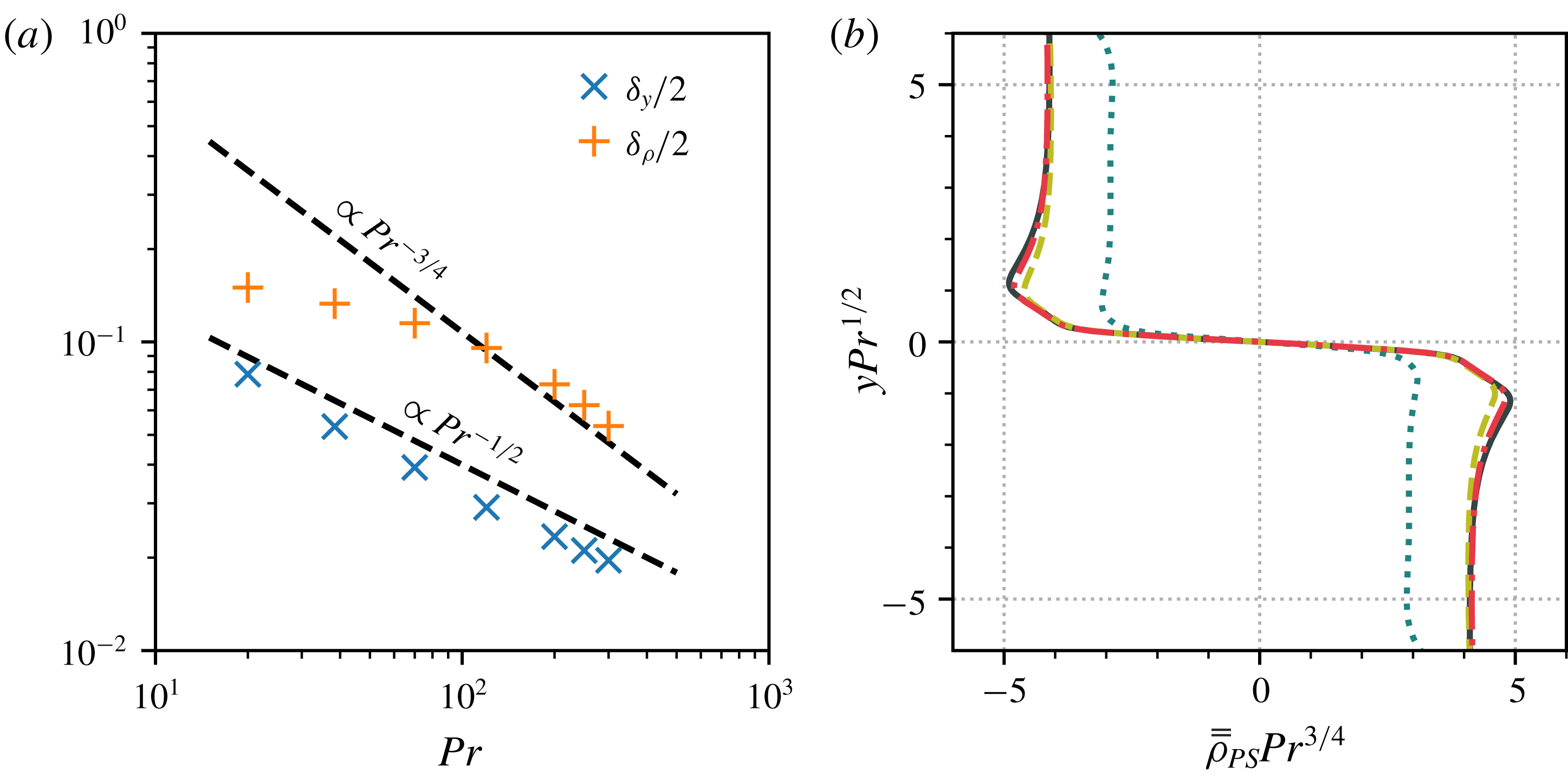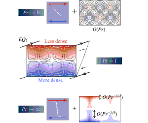


1 Introduction
The identification of numerous unstable invariant solutions in canonical shear flows has played a key role in the modern understanding of transitionally turbulent fluids. These states, most commonly known as exact coherent structures (ECS), underpin a deterministic picture of turbulence in which the flow is viewed as a complicated trajectory through a state space of velocity fields that satisfy the Navier–Stokes equations (Kerswell Reference Kerswell2005; Eckhardt et al. Reference Eckhardt, Schneider, Hof and Westerweel2007; Kawahara, Uhlmann & Van Veen Reference Kawahara, Uhlmann and Van Veen2012). The ECS are simple invariant solutions, equilibria, travelling waves and (relative) periodic orbits, that organise this state space through their stable and unstable manifolds. Though their unstable eigendirections prohibit them from being physically realised, turbulent flows may pass nearby to them. Consequently, the dynamical influence of ECS on the flow via their invariant manifolds is experimentally observable (Suri et al. Reference Suri, Tithof, Grigoriev and Schatz2017, Reference Suri, Tithof, Grigoriev and Schatz2018) and may be investigated in detail by high-resolution direct numerical simulations (DNS) (Kerswell & Tutty Reference Kerswell and Tutty2007; Gibson, Halcrow & Cvitanović Reference Gibson, Halcrow and Cvitanović2008; Cvitanović & Gibson Reference Cvitanović and Gibson2010; Budanur et al. Reference Budanur, Short, Farazmand, Willis and Cvitanović2017). As such, they have proven useful in investigating both the route to turbulence (Itano & Toh Reference Itano and Toh2001; Skufca, Yorke & Eckhardt Reference Skufca, Yorke and Eckhardt2006; Kerswell & Tutty Reference Kerswell and Tutty2007; Schneider, Eckhardt & Yorke Reference Schneider, Eckhardt and Yorke2007; Mellibovsky et al. Reference Mellibovsky, Meseguer, Schneider and Eckhardt2009; Viswanath & Cvitanović Reference Viswanath and Cvitanović2009; Duguet, Brandt & Larsson Reference Duguet, Brandt and Larsson2010; Schneider, Marinc & Eckhardt Reference Schneider, Marinc and Eckhardt2010; Pringle, Willis & Kerswell Reference Pringle, Willis and Kerswell2012) and its subsequent features (Gibson et al. Reference Gibson, Halcrow and Cvitanović2008; Chandler & Kerswell Reference Chandler and Kerswell2013; Willis, Cvitanović & Avila Reference Willis, Cvitanović and Avila2013; Lucas & Kerswell Reference Lucas and Kerswell2015; Budanur et al. Reference Budanur, Short, Farazmand, Willis and Cvitanović2017).
Past work has focussed largely on understanding ECS in simple shear flows in channels and pipes whose physics can be parametrised by a single dimensionless variable: the Reynolds number
 $Re$
. However, it is common in industrial, environmental and astrophysical flows, for the fluid to be subject to additional (buoyancy) forces due to gradients in density or temperature. In order to understand the role of ECS in such flows, one must therefore catalogue the effect of introducing this extra physics onto these states in homogeneous shear flows. Stratified flows require that at least two additional parameters be accounted for; the bulk Richardson number
 $\mathit{Ri}_{b}$
controls the global level of stratification and the Prandtl number
 $Pr$
sets the ratio of viscosity to density diffusion. While identifying ECS within this augmented parameter space presents a sizeable challenge, it is also an opportunity, since many physically relevant regimes remain unexplored.
A number of prior studies have investigated ECS in the stably stratified setting, where the bulk density gradient acts to suppress energetically unfavourable vertical motions. Eaves & Caulfield (Reference Eaves and Caulfield2015) considered the effect of weak stratification on a particular state lying on the laminar–turbulent boundary in stratified plane Couette flow, providing a scaling argument which predicted that the usual physical structure of ECS (the SSP/VWI mechanism, see § 2.2 and Hall & Smith Reference Hall and Smith1991; Waleffe Reference Waleffe1997; Hall & Sherwin Reference Hall and Sherwin2010) is disrupted when
 $\mathit{Ri}_{b}=O(Re^{-2})$
. This was subsequently confirmed asymptotically by both Deguchi (Reference Deguchi2017) and Olvera & Kerswell (Reference Olvera and Kerswell2017). The latter study conducted a substantial survey of the
 $Re$
–
 $\mathit{Ri}_{b}$
space for plane Couette flows and
 $Pr=1$
, continuing solution branches for states at
 $\mathit{Ri}_{b}>0$
that connect known unstratified ECS pairs, which can then be tracked into
 $\mathit{Ri}_{b}<0$
(unstable stratification), to bifurcations of sheared Rayleigh–Bénard solutions. They noted that a key effect of increasing stratification is to encourage ECS to localise in one or more directions, conjecturing the existence of fully localised states when
 $\mathit{Ri}_{b}=O(Re^{0})$
. Finally, Lucas et al. discovered ECS in stratified shear flow with a sinusoidal body forcing (Kolmogorov flow). They observed that both equilibria and turbulent DNS form shear and density layers originating from a sequence of linear ‘zig–zag’ instabilities in the (sinusoidal) base flow (Lucas, Caulfield & Kerswell Reference Lucas, Caulfield and Kerswell2017), and converged periodic orbits to study how stratification affects mixing efficiency (Lucas & Caulfield Reference Lucas and Caulfield2017).
Despite this recent progress in the understanding of stratified ECS, a connection with realistic fully turbulent stratified shear flow remains unresolved (although Lucas, Caulfield & Kerswell (Reference Lucas, Caulfield and Kerswell2019) arguably see traces of underlying ECS in recent stratified plane Couette DNS results). In part this is due to the Prandtl number; prior stratified ECS studies have only dealt with unit Prandtl numbers (Eaves & Caulfield Reference Eaves and Caulfield2015; Deguchi Reference Deguchi2017; Lucas & Caulfield Reference Lucas and Caulfield2017; Lucas et al.
Reference Lucas, Caulfield and Kerswell2017; Olvera & Kerswell Reference Olvera and Kerswell2017) and full DNS of stratified shear flow turbulence is restricted in the Prandtl numbers it can access by issues of numerical resolution. However, Prandtl numbers observed in nature span a substantial range of scales, from as low as
 $10^{-7}$
(inside stars) to up to at least
 $10^{23}$
(Earth’s mantle). On a more terrestrial level, temperature in air exhibits a Prandtl number around 0.7 (which is certainly attainable via DNS), whereas salt in water has
 $Pr\approx 700$
(currently unattainable via DNS, save in the
 $\mathit{Ri}_{b}\rightarrow 0$
limit).
This latter case of salt water shear flow turbulence is of particular interest since the structure of turbulence in the oceans governs the mass transport across its depth (Munk Reference Munk1966). As such, significant effort has been put into explaining the mass transport via modelling of the mixing of the density field that the turbulence causes (Linden Reference Linden1979; Caulfield & Peltier Reference Caulfield and Peltier2003; Sutherland et al. Reference Sutherland, Achatz, Caulfield and Klymak2019). Additionally, it has been observed that stratified shear flow turbulence typically organises into well-mixed constant density layers of large vertical extent separated by relatively thin interfacial regions between each layer (Turner Reference Turner1973; Gregg Reference Gregg1980). Layers may appear spontaneously at turbulent Reynolds numbers and have been reproduced in a number of singly diffusive experimental flows (Ruddick, McDougall & Turner Reference Ruddick, McDougall and Turner1989; Park, Whitehead & Gnanadeskian Reference Park, Whitehead and Gnanadeskian1994; Holford & Linden Reference Holford and Linden1999; Oglethorpe, Caulfield & Woods Reference Oglethorpe, Caulfield and Woods2013; Thorpe Reference Thorpe2016). (The doubly diffusive case is also important, but beyond our scope.) The vertical extent of the well-mixed regions is linked to the flow speed and the buoyancy frequency (Thorpe Reference Thorpe2016), but the detailed structure of the layers and the interfaces between them remains an open question, although the ‘sharpness’ of the interfaces appears to increase as the Prandtl number increases (Zhou et al. Reference Zhou, Taylor, Caulfield and Linden2017b ).
Low Prandtl number turbulence is less extensively studied, since fluids with high thermal diffusivities, such as molten metals, are typically difficult to deal with experimentally. However, turbulence arising from shear instabilities in low-
 $Pr$
flows is hypothesised to significantly contribute to the chemical mixing processes within stellar radiation zones (Zahn Reference Zahn1992). Consequently, the value of examining (via analysis and DNS) simple shear flows in this limit has been recognised (Prat & Lignières Reference Prat and Lignières2013; Prat et al.
Reference Prat, Guilet, Viallet and Müller2016; Garaud, Gagnier & Verhoeven Reference Garaud, Gagnier and Verhoeven2017).
Drawing motivation from the above examples and the recent interest in stratified ECS, our plan here is to complement the stratified plane Couette flow study of Olvera & Kerswell (Reference Olvera and Kerswell2017), by probing the
 $\mathit{Ri}_{b}$
–
 $Pr$
space at fixed Reynolds number. We are particularly interested here in the as-yet unexplored limits
 $Pr\ll 1$
and
 $Pr\gg 1$
, which are relevant for understanding astrophysical and geophysical flows respectively. The key questions are: (a) how strong can the bulk stratification be for ECS still to exist; and (b) what is the effect of
 $Pr$
on the structure of solutions?
The outline of the paper is as follows. In § 2, we detail the physical system, the numerical methods used and the necessary underlying theory (SSP/VWI) for exact coherent states in shear flows. We then take the principal solution of Olvera & Kerswell (Reference Olvera and Kerswell2017) and perform parameter continuation in
 $\mathit{Ri}_{b}$
for a wide range of fixed Prandtl numbers (§ 3), allowing us to identify the range of global stratification that states exist for, before splitting our analysis into the low-
 $Pr$
(§ 3.1) and high-
 $Pr$
(§ 3.2) limits. In the low-
 $Pr$
case, we identify and study an asymptotic solution branch onto which all states collapse. For high-
 $Pr$
states, we intriguingly observe the density field splitting into a homogenised region with highly stratified boundary layers at the walls, punctuated by jets of advected density. We conduct an analysis in § 3.2.1 of its structure in the limit of weak stratification, before proceeding in § 3.2.2 to consider increasing
 $\mathit{Ri}_{b}$
. As states leave the weakly stratified regime, their velocity perturbations retreat from the walls, apparently inhibited by the presence of high stratification. Section 4 concludes with a final discussion of these results and presents some preliminary observations of interfaces developing in the channel interior as
 $Pr$
increases at high Reynolds number.
2 Setting
2.1 Stratified plane Couette flow
The setting for this study is plane Couette flow, which is the flow of an incompressible viscous fluid between two infinite parallel plates at
 $y=\pm h$
, moving with velocities
 $\pm U\boldsymbol{e}_{x}$
. The flow velocity is represented as
 $\boldsymbol{u}:=u\boldsymbol{e}_{x}+v\boldsymbol{e}_{y}+w\boldsymbol{e}_{z}$
(where
 $\boldsymbol{e}_{x}$
,
 $\boldsymbol{e}_{y}$
and
 $\boldsymbol{e}_{z}$
indicate the streamwise, wall-normal and spanwise directions respectively) and obeys no-slip boundary conditions at the plates. Gravity is taken to act in the wall-normal direction,
 $\boldsymbol{g}=-g\boldsymbol{e}_{y}$
. Fixed, but differing densities
 $\unicode[STIX]{x1D70C}_{0}\mp \unicode[STIX]{x1D6E5}_{\unicode[STIX]{x1D70C}}$
are imposed at the plates
 $y=\pm h$
, where
 $\unicode[STIX]{x1D6E5}_{\unicode[STIX]{x1D70C}}\ll \unicode[STIX]{x1D70C}_{0}$
so the Boussinesq approximation can be used. The governing equations for the fluid velocity
 $\boldsymbol{u}$
, pressure
 $p$
and density
 $\unicode[STIX]{x1D70C}$
are
 $$\begin{eqnarray}\displaystyle \displaystyle \frac{\unicode[STIX]{x2202}\boldsymbol{u}}{\unicode[STIX]{x2202}t}+\boldsymbol{u}\boldsymbol{\cdot }\unicode[STIX]{x1D735}\boldsymbol{u} & = & \displaystyle -\unicode[STIX]{x1D735}p+\frac{1}{Re}\unicode[STIX]{x1D6FB}^{2}\boldsymbol{u}-\mathit{Ri}_{b}\unicode[STIX]{x1D70C}\boldsymbol{e}_{y},\end{eqnarray}$$
 $$\begin{eqnarray}\displaystyle \displaystyle \unicode[STIX]{x1D735}\boldsymbol{\cdot }\boldsymbol{u} & = & \displaystyle 0,\end{eqnarray}$$
 $$\begin{eqnarray}\displaystyle \displaystyle \frac{\unicode[STIX]{x2202}\unicode[STIX]{x1D70C}}{\unicode[STIX]{x2202}t}+\boldsymbol{u}\boldsymbol{\cdot }\unicode[STIX]{x1D735}\unicode[STIX]{x1D70C} & = & \displaystyle \frac{1}{RePr}\unicode[STIX]{x1D6FB}^{2}\unicode[STIX]{x1D70C},\end{eqnarray}$$
 $U$
,
 $h$
and
 $\unicode[STIX]{x1D6E5}_{\unicode[STIX]{x1D70C}}$
have been used to non-dimensionalise the system (so that the total dimensional density is
 $\unicode[STIX]{x1D70C}_{0}+\unicode[STIX]{x1D6E5}_{\unicode[STIX]{x1D70C}}\unicode[STIX]{x1D70C}$
, for example). The dimensionless parameters
 $Re$
,
 $Pr$
and
 $\mathit{Ri}_{b}$
are the Reynolds, Prandtl and bulk Richardson numbers respectively, defined as
 $$\begin{eqnarray}Re:=\frac{Uh}{\unicode[STIX]{x1D708}},\quad Pr:=\frac{\unicode[STIX]{x1D708}}{\unicode[STIX]{x1D705}},\quad \mathit{Ri}_{b}:=\frac{\unicode[STIX]{x1D6E5}_{\unicode[STIX]{x1D70C}}}{\unicode[STIX]{x1D70C}_{0}}\frac{gh}{U^{2}},\end{eqnarray}$$
where
 $\unicode[STIX]{x1D708}$
is the kinematic viscosity of the fluid and
 $\unicode[STIX]{x1D705}$
is the diffusivity of some density-affecting agent, such as temperature or salt content. The accompanying boundary conditions are
 $u=\pm 1$
,
 $v=0$
,
 $w=0$
,
 $\unicode[STIX]{x1D70C}=\mp 1$
at the walls
 $y=\pm 1$
which, along with (2.1a
)–(2.1c
), admit a steady base flow with linear velocity and density profiles:
 $$\begin{eqnarray}\boldsymbol{u}=y\boldsymbol{e}_{x},\quad p=\mathit{Ri}_{b}y^{2}/2,\quad \unicode[STIX]{x1D70C}=-y.\end{eqnarray}$$
2.2 Self-sustaining process/vortex–wave interaction mechanism
In this study, we analyse unstable equilibrium solutions to (2.1a
)–(2.1c
) that differ from the basic laminar flow. Almost all such states in homogeneous shear flows where the laminar base state is linearly stable arise physically due to the self-sustaining process (SSP) mechanism proposed by Waleffe (Reference Waleffe1997), which was subsequently recognised to be the finite-
 $Re$
manifestation of the vortex–wave interaction (VWI) theory (Hall & Smith Reference Hall and Smith1991; Hall & Sherwin Reference Hall and Sherwin2010). (The state proposed by Smith & Bodonyi (Reference Smith and Bodonyi1982) and recently found numerically by Deguchi & Walton (Reference Deguchi and Walton2013) is one exception.)
The SSP/VWI process relies on three flow structures, rolls, streaks and waves, sustaining each other against dissipation in a closed loop. Streamwise rolls advect the underlying shear causing the streamwise velocity to vary in the spanwise direction, thereby creating streaks, sustained patches of negative or positive streamwise velocity adjustments to the basic shear. If these streaks have large enough amplitude, they are unstable to streamwise-varying waves, which, via the quadratic nonlinearity in (2.1a ), can then energise the original streamwise rolls to close the loop. This process is covered in great detail elsewhere (Hall & Smith Reference Hall and Smith1991; Hamilton, Kim & Waleffe Reference Hamilton, Kim and Waleffe1995; Waleffe Reference Waleffe1997; Hall & Sherwin Reference Hall and Sherwin2010). At asymptotically high Reynolds number, these states have the following structure:
 $$\begin{eqnarray}\displaystyle & u=\bar{u}(y,z)+\cdots +\unicode[STIX]{x1D6FF}^{\prime }(Re)[U(y,z)\text{e}^{\text{i}kx}+\text{c.c.}]+\cdots \,, & \displaystyle\end{eqnarray}$$
 $$\begin{eqnarray}\displaystyle & v=Re^{-1}\bar{v}(y,z)+\cdots +\unicode[STIX]{x1D6FF}^{\prime }(Re)[V(y,z)\text{e}^{\text{i}kx}+\text{c.c.}]+\cdots \,, & \displaystyle\end{eqnarray}$$
 $$\begin{eqnarray}\displaystyle & w=Re^{-1}\bar{w}(y,z)+\cdots +\unicode[STIX]{x1D6FF}^{\prime }(Re)[W(y,z)\text{e}^{\text{i}kx}+\text{c.c.}]+\cdots \,, & \displaystyle\end{eqnarray}$$
 $$\begin{eqnarray}\displaystyle & p=Re^{-2}\bar{p}(y,z)+\cdots +\unicode[STIX]{x1D6FF}^{\prime }(Re)[P(y,z)\text{e}^{\text{i}kx}+\text{c.c.}]+\cdots \,, & \displaystyle\end{eqnarray}$$
 $\unicode[STIX]{x1D6FF}^{\prime }(Re)=Re^{-7/6}$
, except in the
 $O(Re^{-1/3})$
-thick critical layer (located where the laminar base flow vanishes for equilibria), where it is
 $Re^{-5/6}$
(Hall & Sherwin Reference Hall and Sherwin2010). Here,
 $$\begin{eqnarray}\bar{q}:=\frac{1}{L_{x}}\int _{0}^{L_{x}}q\,\text{d}x\end{eqnarray}$$
denotes the streamwise average of a given flow field
 $q$
. In these expressions,
 $(\bar{u},0,0)$
represents the streak-modified base shear,
 $(0,\bar{v},\bar{w})$
the streamwise rolls and
 $(U,V,W)$
the amplitudes of the streamwise-varying wave field.
Although strictly valid only in the high-
 $Re$
limit, VWI captures the physics of SSP remarkably well, all the way down to transitionally turbulent
 $Re$
(Hall & Sherwin Reference Hall and Sherwin2010), which is the regime considered in the bulk of this study. The theory has been extended in the stratified setting by Hall (Reference Hall2012), to incorporate plane Couette flows with a buoyancy force aligned with the streamwise direction. Later, Deguchi (Reference Deguchi2017) and Olvera & Kerswell (Reference Olvera and Kerswell2017) considered the vortex–wave interaction for the situation herein with buoyancy in the wall-normal direction, presenting numerical calculations at varying
 $Re$
and fixed
 $Pr=1$
. In this study, we use the VWI scalings in (2.4a
)–(2.4d
) to look at the effect of varying
 $Pr$
on states at fixed
 $Re$
.
2.3 Numerical methods
The numerical solutions presented below were obtained primarily using a bespoke pseudo-spectral code that computes steady solutions of (2.1a
)–(2.1c
), in the box
 $(x,y,z)\in [0,\,L_{x}]\times [-1,1]\times [0,\,L_{z}]$
, with periodic streamwise and spanwise directions of lengths
 $L_{x}$
and
 $L_{z}$
respectively. The standard Newton–Raphson method was used to converge equilibria, with lower-upper (LU) decomposition to invert the full discretised system Jacobian.
The additional solutions in § 3.2.3 were obtained using a modified version of the Channelflow 2.0 DNS software (Gibson et al.
Reference Gibson, Reetz, Azimi, Ferraro, Kreilos, Schrobsdorff, Farano, Yesil, Schütz and Culpo2019) that employs a matrix-free iterative solver to find invariant solutions via two standard methods: Stokes preconditioning (Tuckerman Reference Tuckerman1989) and time integration (Viswanath Reference Viswanath2007; Gibson et al.
Reference Gibson, Halcrow and Cvitanović2008). The former method was used to the compute
 $Pr\lesssim 10$
solutions in § 3.2.3 and the latter was used at higher
 $Pr$
, where the Stokes-preconditioned system suffers the effects of poorer numerical conditioning more acutely (Tuckerman, Langham & Willis Reference Tuckerman, Langham and Willis2019).
Provided enough computer memory is available, we find that our bespoke solver is typically preferable to the standard iterative schemes. The reason is twofold: firstly, there is no need to perform multiple expensive time integrations to compute states. (Though we note that the recent parallelisation of the Channelflow code, see Gibson et al. (Reference Gibson, Reetz, Azimi, Ferraro, Kreilos, Schrobsdorff, Farano, Yesil, Schütz and Culpo2019), has made time integration much more attractive, paving the way for fast ECS computations with very high spatial resolutions.) Secondly, we restrict solutions to a highly symmetric subspace, thereby reducing the size of the basis set needed to represent the states at a given spatial resolution and substantially decreasing the cost of an exact matrix inversion. See appendix A for technical details. Following the previous work (Deguchi Reference Deguchi2017; Olvera & Kerswell Reference Olvera and Kerswell2017), the symmetries imposed (in addition to
 $L_{x}$
- and
 $L_{z}$
-periodicity) are: ‘shift-and-reflect’
 ${\mathcal{S}}$
, rotation about the
 $z$
-axis
 $\unicode[STIX]{x1D6FA}$
and spanwise reflection
 ${\mathcal{Z}}$
, defined by
 $$\begin{eqnarray}\displaystyle & {\mathcal{S}}:[u,v,w,p,\unicode[STIX]{x1D70C}](x,y,z)\mapsto [u,v,-w,p,\unicode[STIX]{x1D70C}](x+L_{x}/2,y,L_{z}/2-z), & \displaystyle\end{eqnarray}$$
 $$\begin{eqnarray}\displaystyle & \unicode[STIX]{x1D6FA}:[u,v,w,p,\unicode[STIX]{x1D70C}](x,y,z)\mapsto [-u,-v,w,p,-\unicode[STIX]{x1D70C}](-x,-y,z), & \displaystyle\end{eqnarray}$$
 $$\begin{eqnarray}\displaystyle & {\mathcal{Z}}:[u,v,w,p,\unicode[STIX]{x1D70C}](x,y,z)\mapsto [u,v,-w,p,\unicode[STIX]{x1D70C}](x,y,-z). & \displaystyle\end{eqnarray}$$
 ${\mathcal{S}}$
, possess an additional spanwise reflection symmetry in the line
 $z=\unicode[STIX]{x03C0}/4$
. This implies that the cells
 $[-1,1]\times [0,L_{z}/2]$
and
 $[-1,1]\times [L_{z}/2,L_{z}]$
are identical and obey reflection symmetries along the lines
 $z=\unicode[STIX]{x03C0}/4$
and
 $z=3\unicode[STIX]{x03C0}/4$
respectively.
The majority of the results presented involve a single
 ${\mathcal{S}}$
-,
 $\unicode[STIX]{x1D6FA}$
- and
 ${\mathcal{Z}}$
-symmetric solution family described at the beginning of § 3 and were computed with the direct solver in a domain with
 $L_{x}=2\unicode[STIX]{x03C0}$
and
 $L_{z}=\unicode[STIX]{x03C0}$
, at
 $Re=400$
. Channelflow was later employed to obtain the additional § 3.2.3 equilibria in a box with
 $L_{x}=2\unicode[STIX]{x03C0}/1.14$
,
 $L_{z}=2\unicode[STIX]{x03C0}/2.5$
,
 $Re=400$
and to cross-check a sample of solutions from the direct solver. It is worth mentioning here, that in both cases, these results demanded very high numerical resolutions. Indeed, the §§ 3.2 and 3.2.3 solutions at high Prandtl number may represent some of the most highly resolved ECS converged to date. Further details, including typical resolutions achieved are given in appendix A.
Both codes are coupled to a pseudo-arclength continuation algorithm that enables straightforward computation of solution families parametrised by
 $Re$
,
 $\mathit{Ri}_{b}$
or
 $Pr$
. This allows us to track solution curves which, for the ECS studied herein, arise via saddle-node bifurcations (Gibson, Halcrow & Cvitanović Reference Gibson, Halcrow and Cvitanović2009) with distinct upper and lower branches. (The lower branch lies closest to the laminar base state in any reasonable metric, e.g. energy, dissipation, amplitude.) Since multiple equilibria may exist at the same point in parameter space, we use the ‘surplus’ mean wall stress
 $$\begin{eqnarray}\unicode[STIX]{x1D70F}_{y}:=\left.\frac{1}{L_{x}L_{z}}\int _{0}^{L_{x}}\int _{0}^{L_{z}}\frac{\unicode[STIX]{x2202}u}{\unicode[STIX]{x2202}y}\right|_{y=1}\,\text{d}x\,\text{d}z-1,\end{eqnarray}$$
to distinguish between them (where
 $\unicode[STIX]{x1D70F}_{y}=0$
for the base flow).
3 Results
This study focusses mainly on a lower-branch equilibrium solution originally discovered by Itano & Generalis (Reference Itano and Generalis2009), who computed it via homotopy from a solution in an unstably stratified channel with stationary walls and Gibson et al. (Reference Gibson, Halcrow and Cvitanović2009), who independently converged it from snapshots of a transitionally turbulent flow simulation. We follow the nomenclature used by Gibson et al. (Reference Gibson, Halcrow and Cvitanović2009), whose search identified 13 different equilibria and named them
 $EQ_{1}$
–
 $EQ_{13}$
. Our chosen solution is
 $EQ_{7}$
and its upper-branch counterpart
 $EQ_{8}$
. In the vertically stratified case with
 $Pr=1$
,
 $EQ_{7}$
was recently studied by Olvera & Kerswell (Reference Olvera and Kerswell2017), who observed that it lies on the so-called edge manifold separating laminar and turbulent dynamics and is therefore likely to play a role in organising the transition process. In § 3.2.3 we briefly address other equilibrium solutions.
Spanwise cross-sections of the
 $EQ_{7}$
state at
 $Re=400$
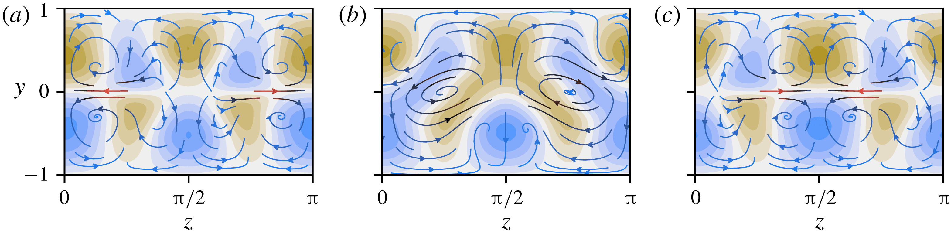
without stratification. The plots show the streamwise velocity perturbation
 $\hat{u} :=u-y$
, plotted using 11 equally spaced contour intervals between
 $-0.22$
(brown) and 0.22 (blue). The middle interval is centred at zero (white). Overlaid are streamlines of the
 $(v,w)$
-field, coloured with a linear gradient from blue to red according to the magnitude of in-plane velocity, which lies in the interval
 $[0,0.077)$
. Three
 $(y,z)$
-slices are given, at
 $x=0$
,
 $x=\unicode[STIX]{x03C0}/2$
and
 $x=\unicode[STIX]{x03C0}$
(a–c), covering half the computational domain.

Figure 1 shows
 $yz$
-contours of the perturbation to the laminar base flow
 $\hat{u} :=u-y$
, for
 $EQ_{7}$
with no imposed stratification. Also shown are
 $(v,w)$
-streamlines, coloured from blue to red according to the speed of the flow in the plane. The leftmost panel is a slice through
 $x=0$
. It contains two rows of four streaks, separated by the centre line
 $y=0$
. The in-plane streamlines provide insight into the formation of the streaks. For example, the negative (brown) streak centred at approximately
 $(z,y)=(\unicode[STIX]{x03C0}/4,-0.5)$
arises due to uplift of negative streamwise velocity from the laminar base flow near the lower wall. Likewise, the other streaks emerge at regions of inflow and outflow from the boundaries, with the strongest in-plane advection accounting for the largest streaks, centred along the line
 $z=0\equiv \unicode[STIX]{x03C0}$
. In the middle panel at
 $x=\unicode[STIX]{x03C0}/2$
, there is transport between the upper and lower half-channels due to vortices centred at
 $(\unicode[STIX]{x03C0}/4,0)$
and
 $(3\unicode[STIX]{x03C0}/4,0)$
and some of the streaks have merged into larger structures. The final panel at
 $x=\unicode[STIX]{x03C0}=L_{x}/2$
is dictated by the imposed symmetries (specifically
 ${\mathcal{S}}$
and
 ${\mathcal{Z}}$
), which constrain it to be equal to an
 $L_{z}/2$
-spanwise shift of the
 $x=0$
slice. Likewise, the remainder of the computational domain,
 $\unicode[STIX]{x03C0}<x\leqslant 2\unicode[STIX]{x03C0}$
, is determined this way. Slices at intermediate streamwise coordinates gradually interpolate between the panels shown and all the states considered herein possess either a similar, or lower level of streamwise variation. Therefore, in the following we only use slices at
 $x=0$
and
 $\unicode[STIX]{x03C0}/2$
to visualise states or, more commonly take a streamwise average.
To examine how
 $EQ_{7}$
(and where possible,
 $EQ_{8}$
) is affected by varying the Prandtl number, a pseudo-arclength continuation algorithm was used to converge states at fixed
 $Re=400$
and varying
 $Pr$
and
 $\mathit{Ri}_{b}$
. Starting with initial parameters
 $Pr=1$
,
 $\mathit{Ri}_{b}=0$
, continuation was first performed on
 $Pr$
in both directions to obtain solutions with a wide spread of Prandtl numbers ranging from
 $Pr=10^{-4}$
to
 $Pr=500$
. The character of these states depends strongly on whether the Prandtl number is significantly less or greater than unity and we divide our study along these lines.
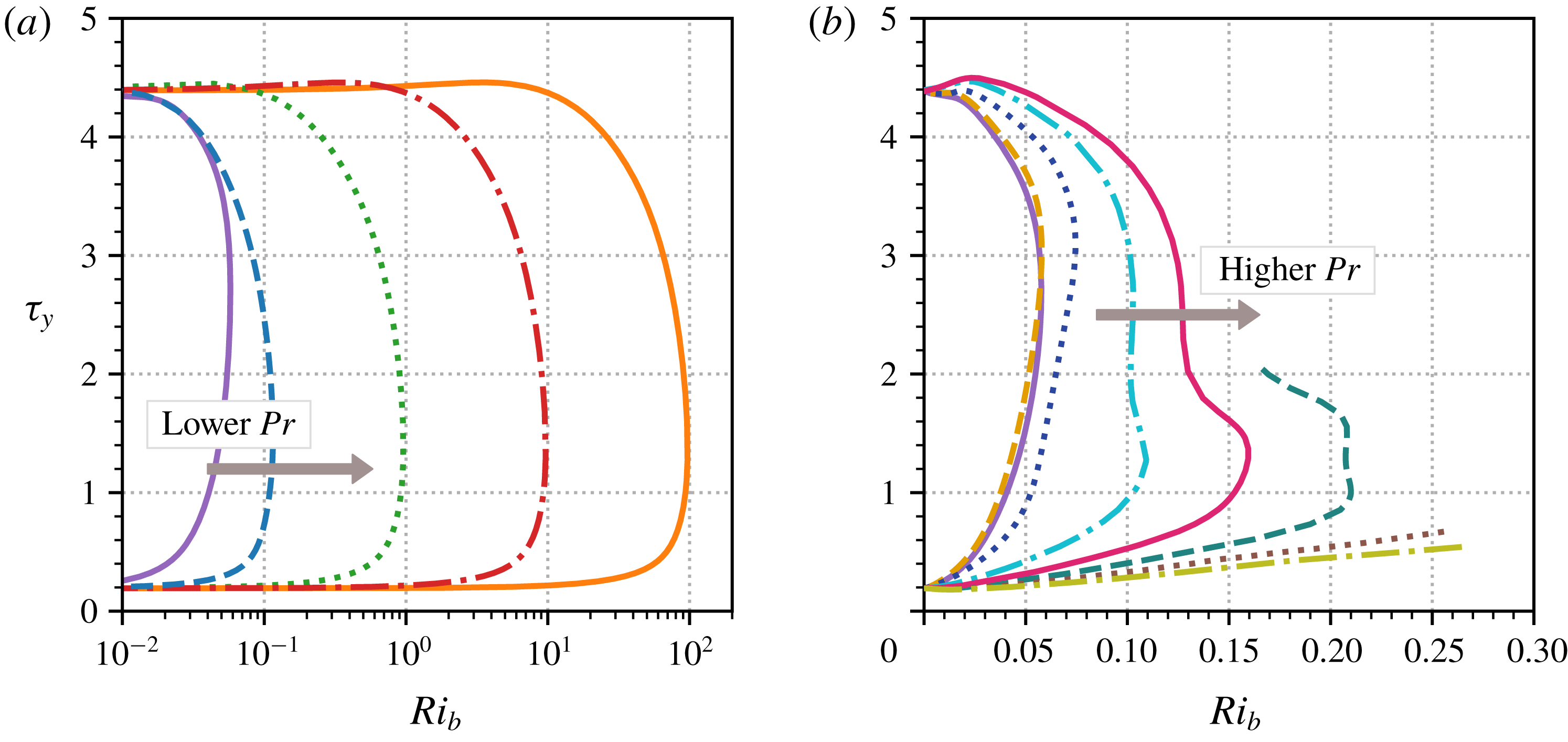
Parameter continuation curves for the
 $EQ_{7}$
(lower)/
 $EQ_{8}$
(upper) states in terms of the bulk Richardson number and mean wall stress
 $\unicode[STIX]{x1D70F}_{y}$
for different Prandtl numbers. (a) Low-
 $Pr$
states:
 $Pr=10^{0}$
(purple solid),
 $Pr=10^{-1}$
(blue dashed),
 $Pr=10^{-2}$
(green dotted),
 $Pr=10^{-3}$
(red dash-dot) and
 $Pr=10^{-4}$
(orange solid). The bifurcation point of the
 $Pr=10^{-4}$
curve is at
 $\mathit{Ri}_{b}\approx 97$
. (b) Higher-
 $Pr$
states:
 $Pr=1$
(purple solid), 2 (yellow dashed), 7 (navy dotted), 20 (cyan dash-dot), 40 (magenta solid), 70 (teal dashed), 120 (brown dotted), 200 (olive dash-dot).

Figure 2 shows solution branches of the
 $EQ_{7}$
and
 $EQ_{8}$
states, obtained by starting with the states at
 $Pr=10^{-4}$
to
 $200$
and continuing them in
 $\mathit{Ri}_{b}$
. Part (a) plots the continuation curves for
 $Pr\leqslant 1$
. All five curves are similar, possessing the familiar shape of a saddle-node bifurcation. Starting from
 $\mathit{Ri}_{b}=0$
, both lower and upper branches enter an initial regime (present, but not shown for
 $Pr=1$
) where their mean wall stress is unaffected by the presence of global stratification. This is followed by a transition between solution branches where the stress changes comparatively rapidly. The range of admissible bulk Richardson numbers increases dramatically as
 $Pr$
decreases, suggesting that in the limit of low
 $Pr$
, ECS are insensitive to stratification and may persist up to arbitrarily high
 $\mathit{Ri}_{b}$
as
 $Pr$
is reduced.
Figure 2(b) shows the
 $Pr\geqslant 1$
continuation curves. The
 $Pr=1$
, 2 and 7 curves have essentially the same shape as the low-
 $Pr$
curves. At higher
 $Pr$
, the solution branches follow the opposite trend to the low-
 $Pr$
case, reaching progressively higher
 $\mathit{Ri}_{b}$
as the Prandtl number increases. Another trend to note is that the upper branches reach increasingly higher mean wall stresses than
 $EQ_{8}$
itself. The
 $Pr\geqslant 40$
curves required high numerical resolution to be continued reliably, for reasons which shall become clear in § 3.2. The three highest
 $Pr$
curves, which terminate before reaching
 $EQ_{8}$
, were continued as far as available computational resources permitted, the final two not reaching their saddle-node bifurcations. Nevertheless, the
 $Pr=70$
, 120 and 200 curves persist up to at least
 $\mathit{Ri}_{b}=0.21$
, 0.26 and 0.27 respectively. This trend along the lower branch suggests that
 $EQ_{7}$
might admit arbitrarily large global stratification in the high-
 $Pr$
limit. We now analyse the solutions of figure 2 in the two defined limits.
3.1 Low Prandtl number (
 $Pr\ll 1$
)

At low
 $Pr$
, density transport in the fluid is diffusion dominated and as a result
 $\unicode[STIX]{x1D70C}$
should not develop small scales or deviate far from the basic state. To reflect at least the latter, we consider the expansion
 $\unicode[STIX]{x1D70C}(x,y,z)=-y+\unicode[STIX]{x1D700}\unicode[STIX]{x1D70C}_{1}(x,y,z)+\cdots \,$
, where
 $\unicode[STIX]{x1D700}$
is a small parameter to be determined, with
 $\unicode[STIX]{x1D70C}_{1}=O(Pr^{0})$
. This is certainly true at either end of the continuation curves in figure 2(a) where
 $\mathit{Ri}_{b}\rightarrow 0$
, but will be found to be true over the whole curve. Working with the perturbations to the laminar base state
 $\hat{u} :=u-y$
,
 $\hat{v}:=v$
,
 ${\hat{w}}:=w$
,
 $\hat{p}:=p-\mathit{Ri}_{b}y^{2}/2$
and
 $\hat{\unicode[STIX]{x1D70C}}:=\unicode[STIX]{x1D70C}+y=\unicode[STIX]{x1D700}\unicode[STIX]{x1D70C}_{1}+\cdots \,$
, the steady form of (2.1c
) becomes
 $$\begin{eqnarray}\unicode[STIX]{x1D700}(y+\hat{u} )\frac{\unicode[STIX]{x2202}\unicode[STIX]{x1D70C}_{1}}{\unicode[STIX]{x2202}x}+\hat{v}\left(-1+\unicode[STIX]{x1D700}\frac{\unicode[STIX]{x2202}\unicode[STIX]{x1D70C}_{1}}{\unicode[STIX]{x2202}y}\right)+\unicode[STIX]{x1D700}{\hat{w}}\frac{\unicode[STIX]{x2202}\unicode[STIX]{x1D70C}_{1}}{\unicode[STIX]{x2202}z}=\frac{\unicode[STIX]{x1D700}}{RePr}\unicode[STIX]{x1D6FB}^{2}\unicode[STIX]{x1D70C}_{1},\end{eqnarray}$$
after neglecting
 $O(\unicode[STIX]{x1D700}^{2})$
terms. We now determine the leading-order velocity fields in (3.1) from the asymptotic VWI structure in (2.4a
)–(2.4d
). The cross-stream velocity
 $\hat{v}$
is largest for the wave field in the critical layer, but because of the enhanced gradients of
 $O(Re^{1/3})$
across this region, this flow actually drives a smaller density field of
 $O(\unicode[STIX]{x1D700}Re^{-1/2})$
than the streamwise rolls outside the critical layer, which drive an
 $O(\unicode[STIX]{x1D700})$
density field. Therefore, the leading-order physics is away from the critical layer, so that
 $\hat{v}=\bar{v}(y,z)/Re$
and
 ${\hat{w}}=\bar{w}(y,z)/Re$
and (3.1) can be rewritten as
 $$\begin{eqnarray}\bar{v}\left(-1+\unicode[STIX]{x1D700}\frac{\unicode[STIX]{x2202}\unicode[STIX]{x1D70C}_{1}}{\unicode[STIX]{x2202}y}\right)+\unicode[STIX]{x1D700}\bar{w}\frac{\unicode[STIX]{x2202}\unicode[STIX]{x1D70C}_{1}}{\unicode[STIX]{x2202}z}=\frac{\unicode[STIX]{x1D700}}{Pr}\unicode[STIX]{x1D6FB}^{2}\unicode[STIX]{x1D70C}_{1},\end{eqnarray}$$
where, because the driving term is streamwise independent,
 $\unicode[STIX]{x1D70C}_{1}=\unicode[STIX]{x1D70C}_{1}(y,z)$
and the streamwise advection term drops. This then leads to
 $\unicode[STIX]{x1D700}=Pr\ll 1$
and the leading equation
 $$\begin{eqnarray}-\bar{v}=\unicode[STIX]{x1D6FB}^{2}\unicode[STIX]{x1D70C}_{1}.\end{eqnarray}$$
Inverting this relationship, the leading density perturbation
 $\hat{\unicode[STIX]{x1D70C}}=-RePr\unicode[STIX]{x1D6E5}^{-1}\hat{v}$
(where
 $\unicode[STIX]{x1D6E5}:=\unicode[STIX]{x1D6FB}^{2}$
) can then be eliminated from the Navier–Stokes equations to leave the low-
 $Pr$
equations (or low-Péclet number equations, see Lignières Reference Lignières1999),
 $$\begin{eqnarray}\displaystyle & (y+\hat{u} )\hat{u} _{x}+\hat{v}(1+\hat{u} _{y})+{\hat{w}}\hat{u} _{z}+\hat{p}_{x}=Re^{-1}\unicode[STIX]{x1D6FB}^{2}\hat{u} , & \displaystyle\end{eqnarray}$$
 $$\begin{eqnarray}\displaystyle & (y+\hat{u} )\hat{v}_{x}+\hat{v}\hat{v}_{y}+{\hat{w}}\hat{v}_{z}+\hat{p}_{y}=Re^{-1}[\unicode[STIX]{x1D6FB}^{2}+\mathit{Ri}_{b}PrRe^{2}\unicode[STIX]{x1D6E5}^{-1}]\hat{v}, & \displaystyle\end{eqnarray}$$
 $$\begin{eqnarray}\displaystyle & (y+\hat{u} ){\hat{w}}_{x}+\hat{v}{\hat{w}}_{y}+{\hat{w}}{\hat{w}}_{z}+\hat{p}_{z}=Re^{-1}\unicode[STIX]{x1D6FB}^{2}{\hat{w}}, & \displaystyle\end{eqnarray}$$
 $$\begin{eqnarray}\displaystyle & \hat{u} _{x}+\hat{v}_{y}+{\hat{w}}_{z}=0. & \displaystyle\end{eqnarray}$$
 $\mathit{Ri}_{b}$
and the Prandtl number
 $Pr$
in the combination
 $\mathit{Ri}_{b}Pr$
. Furthermore, the cross-stream momentum equation, equation (3.4b
), also implies that there exists a region of weakly stratified (small
 $\mathit{Ri}_{b}$
) flow where the Navier–Stokes and the density equations remain effectively uncoupled until
 $\mathit{Ri}_{b}=O(Pr^{-1}Re^{-2})$
. These are the flat regions of both the upper and lower solution branches in figure 2(a), where increasing
 $\mathit{Ri}_{b}$
has no effect on
 $\unicode[STIX]{x1D70F}_{y}$
. As
 $Pr\rightarrow 0$
, these regions extend to
 $\mathit{Ri}_{b}\sim O(1/Pr)$
.
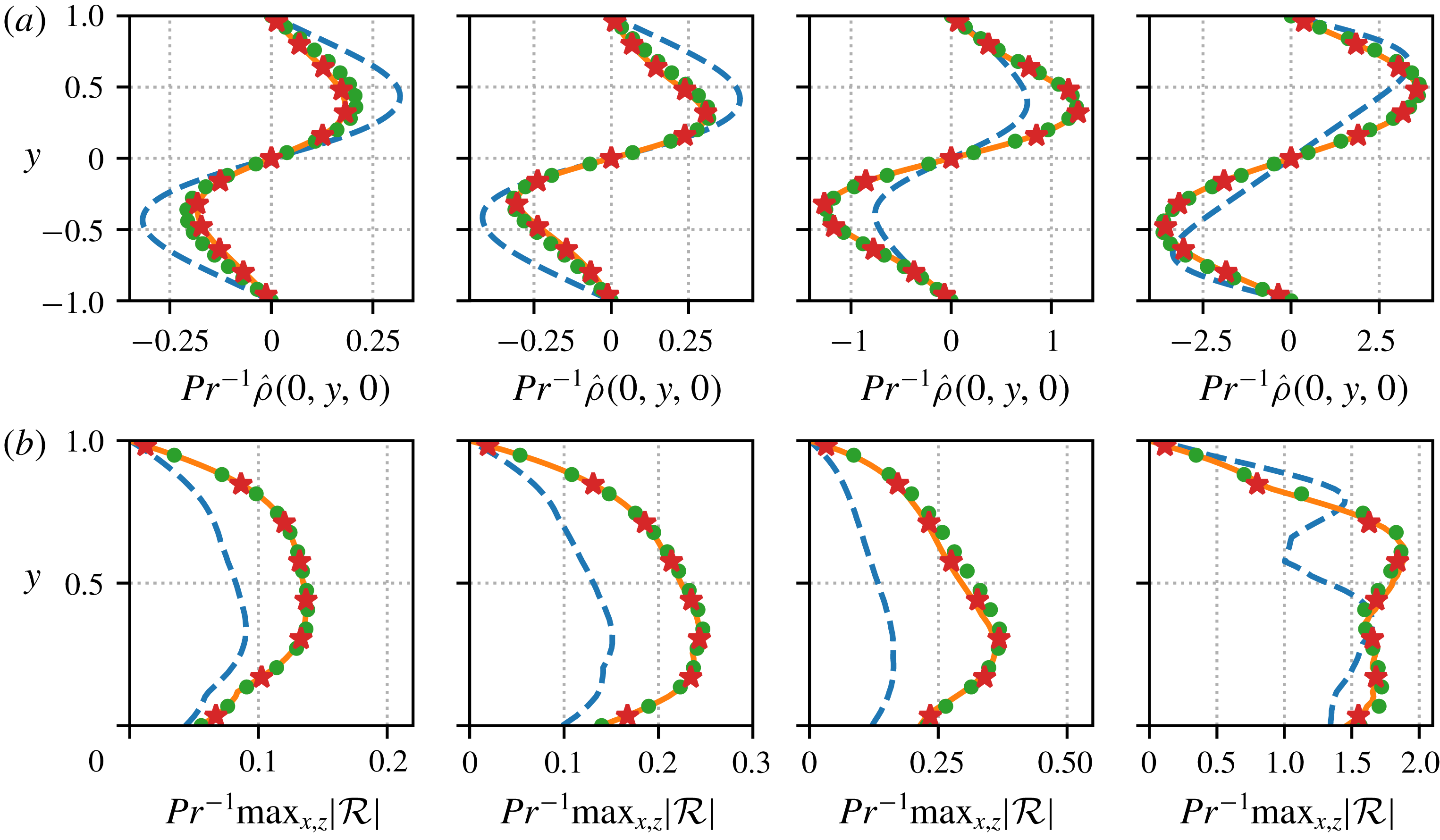
Verification of the
 $O(Pr)$
scalings predicted for low Prandtl number ECS. In all plots the Prandtl numbers are
 $Pr=10^{-1}$
(blue dashed),
 $Pr=10^{-2}$
(green circles)
 $Pr=10^{-3}$
(red stars) and
 $Pr=10^{-4}$
(orange solid). Across each column
 $Pr\mathit{Ri}_{b}$
is fixed at a given point along the solution curves plotted in figure 4(a). From left to right:
 $Pr\mathit{Ri}_{b}=0$
,
 $0.005$
(lower branch),
 $0.097$
(saddle-node) and
 $0.005$
(upper branch). (a) Cross-channel profiles of
 $\hat{\unicode[STIX]{x1D70C}}$
, for
 $x,z=0$
, rescaled by
 $Pr^{-1}$
. (b) Absolute maximum values along streamwise and spanwise directions of
 ${\mathcal{R}}:=\hat{v}+\unicode[STIX]{x1D6FB}^{2}\hat{\unicode[STIX]{x1D70C}}/(RePr)$
, rescaled by
 $Pr^{-1}$
.

This scaling result,
 $\mathit{Ri}_{b}=O(Pr^{-1}Re^{-2})$
, equivalent to the Rayleigh number
 $\mathit{Ra}:=-\mathit{Ri}_{b}PrRe^{2}$
being
 $O(1)$
, was first observed numerically in the
 $Pr=1$
case by Eaves & Caulfield (Reference Eaves and Caulfield2015) and then in the analysis of Deguchi (Reference Deguchi2017) and Olvera & Kerswell (Reference Olvera and Kerswell2017). There, at least for
 $Pr=O(1)$
, once the stratification strength increases beyond this scaling, new dynamic balances emerge (e.g. ‘regime 2’ in Olvera & Kerswell (Reference Olvera and Kerswell2017), ultimately followed by the ‘unit Reynolds number Navier–Stokes’ (UNS) regime of Deguchi (Reference Deguchi2017) or ‘regime 3’ of Olvera & Kerswell (Reference Olvera and Kerswell2017)). Here however, in the
 $Pr\rightarrow 0$
limit this is not the case. In figure 3(a), we demonstrate that the
 $O(Pr)$
scaling of the density perturbation persists along the whole length of the solution curves. The leftmost figure verifies the situation for
 $EQ_{7}$
at
 $\mathit{Ri}_{b}=0$
(where the stratification is still present but the buoyancy force is switched off), plotting
 $Pr^{-1}\hat{\unicode[STIX]{x1D70C}}$
as a function of
 $y$
for
 $x,z=0$
. These slices, taken from solutions at
 $Pr=10^{-1},10^{-2},10^{-3}$
and
 $10^{-4}$
, collapse neatly onto an asymptotic profile for
 $Pr\gtrsim 10^{-2}$
. The subsequent plots confirm that the same holds for
 $\mathit{Ri}_{b}>0$
solutions using the same Prandtl numbers, at various points along the solution branches, now keeping the size of the buoyancy forcing constant. This property is not specific to our choice of
 $x$
,
 $z=0$
. We have checked that the scalings are observed for profiles with
 $x=0$
,
 $\unicode[STIX]{x03C0}/4$
,
 $\unicode[STIX]{x03C0}/2$
,
 $3\unicode[STIX]{x03C0}/4$
and
 $z=0$
,
 $\unicode[STIX]{x03C0}/2$
.
In figure 3(b), we plot
 $\max _{x,z}|\hat{v}+\unicode[STIX]{x1D6FB}^{2}\hat{\unicode[STIX]{x1D70C}}/(RePr)|$
at the same points along the solution curves as in figure 3(a). These curves collapse upon rescaling by
 $Pr^{-1}$
, confirming that (3.3) is obeyed up to an
 $O(\unicode[STIX]{x1D700})$
error term across the whole domain, as implied by (3.2). The conclusion is then that solutions should be self-similar in the limit of low
 $Pr$
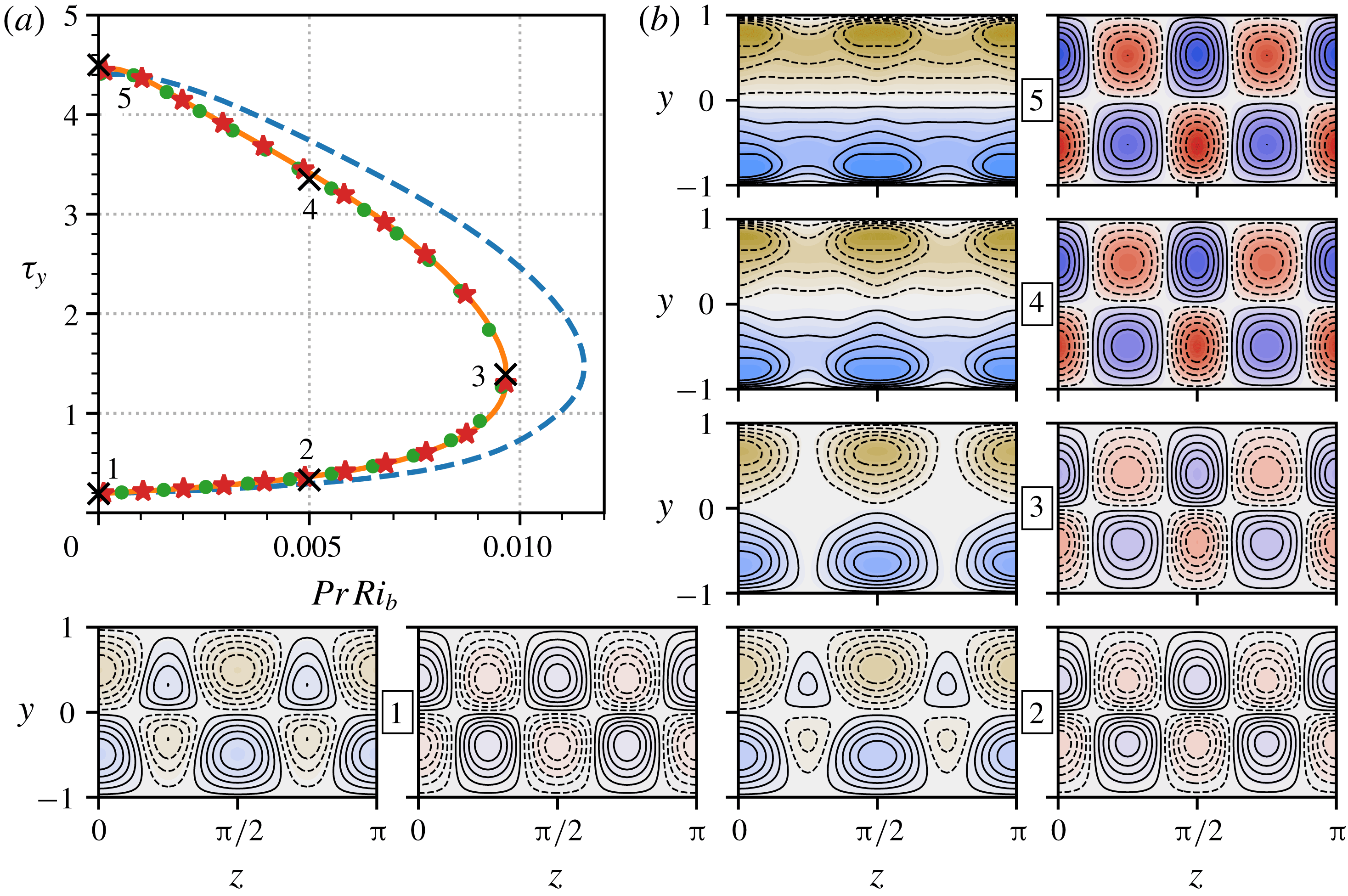
along the whole solution curve. Figure 4(a) replots the parameter continuation curves in figure 2(a) against
 $\mathit{Ri}_{b}Pr$
, confirming the collapse onto a single asymptotic branch. In particular, this implies that the maximum bulk Richardson number for these solutions is
 $\mathit{Ri}_{b}^{m}\approx 0.01/Pr$
at
 $Re=400$
as
 $Pr\rightarrow 0$
.
Self-similar solution branches of
 $EQ_{7}$
(lower)/
 $EQ_{8}$
(upper) in the
 $Pr\rightarrow 0$
limit. (a) Parameter continuation curves in bulk Richardson number as a function of mean wall stress. The horizontal axis has been rescaled by
 $Pr$
causing the curves to collapse. The Prandtl numbers match those in figure 3. (b) Pairs of contour plots along the
 $Pr=10^{-4}$
branch (orange solid), numbered according to the labelled points in part (a). Left-hand plots show the streamwise average of
 $\hat{u}$
, shaded between
 $-0.8$
(brown) and 0.8 (blue). Right-hand plots show the streamwise average of the
 $\hat{\unicode[STIX]{x1D70C}}$
field, shaded between
 $-2.3\times 10^{-4}$
(red) and
 $2.3\times 10^{-4}$
(blue). In all plots, the middle contour interval is white and centred at zero; black contour lines are overlaid to show the structure of solutions, using 11 equally spaced intervals, between
 $\pm \max _{y,z}|\bar{u}-y|$
or
 $\pm \max _{y,z}|\bar{\unicode[STIX]{x1D70C}}|$
for each field, as appropriate. Dashed lines are negative contours and solid lines are positive. Anti-clockwise from bottom left:
 $Pr\mathit{Ri}_{b}=0$
(
 $EQ_{7}$
, point 1), 0.005 (point 2), 0.097 (saddle-node, point 3), 0.005 (point 4), 0 (
 $EQ_{8}$
, point 5).

Contour plots of
 $\bar{v}(y,z)$
along the
 $Pr=10^{-4}$
solution branch, at the numbered points indicated in figure 4(a): from (a) to (c), the plots correspond to the first (
 $EQ_{7}$
), third (saddle-node) and fifth (
 $EQ_{8}$
) solution pairs in figure 4(b). The contours are shaded between
 $-0.19$
(pink) and 0.19 (cyan); black contour lines are overlaid using 11 equally spaced intervals, between
 $\pm \max _{y,z}|\bar{v}|$
, which equals 0.014, 0.076 and 0.19 respectively. Dashed contours indicate
 $\bar{v}<0$
, solid contours
 $\bar{v}>0$
.

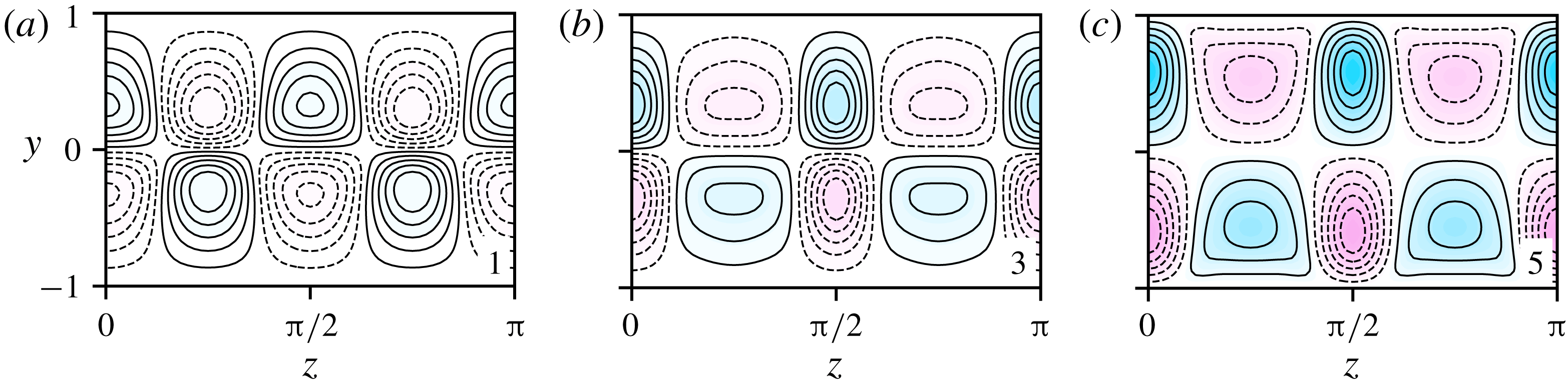
In figure 4(b) we plot contour slices through the
 $yz$
-plane along the
 $Pr=10^{-4}$
curve. The contour plots are organised in numbered side-by-side pairs, showing streamwise averages of
 $\hat{u}$
on the left and
 $\hat{\unicode[STIX]{x1D70C}}$
on the right. Along the lower branch (plots 1–3) we see that the streaks centred at
 $z=\unicode[STIX]{x03C0}/4$
and
 $3\unicode[STIX]{x03C0}/4$
shrink as
 $\mathit{Ri}_{b}$
increases. At the saddle node (plot 4) they have disappeared completely and the mean
 $\hat{u}$
field becomes separated into negative (upper) and positive (lower) halves. This can be traced to the
 $\hat{v}$
field, which feeds these streaks by advecting the base shear; its streamwise average is plotted in figure 5. (For reference, the corresponding roll streamlines are included in figure 6.) As the state transitions from the less energetic
 $EQ_{7}$
state toward the more energetic
 $EQ_{8}$
, the overall strength of the
 $\hat{v}$
field increases (as do the magnitudes of
 $\hat{u}$
and
 $\hat{\unicode[STIX]{x1D70C}}$
, which are driven by
 $\hat{v}$
). However, the increased buoyancy force from point 1 to point 3 penalises upward motion wherever
 $\hat{\unicode[STIX]{x1D70C}}>0$
and downward motion where
 $\hat{\unicode[STIX]{x1D70C}}<0$
. Consequently, there is a redistribution of the
 $\hat{v}$
field along the lower branch, diminishing in regions where the signs of
 $\hat{v}$
and
 $\hat{\unicode[STIX]{x1D70C}}$
match (outflow from the walls) and concentrating where they differ (inflow to the walls). This leads to the (inflow) streaks centred at
 $z=0\equiv \unicode[STIX]{x03C0}$
and
 $\unicode[STIX]{x03C0}/2$
becoming increasingly dominant. This division persists along much of the upper branch, connecting through to the
 $EQ_{8}$
solution where the unevenly distributed wall-normal velocity field and corresponding streak structure exist in the unstratified setting.
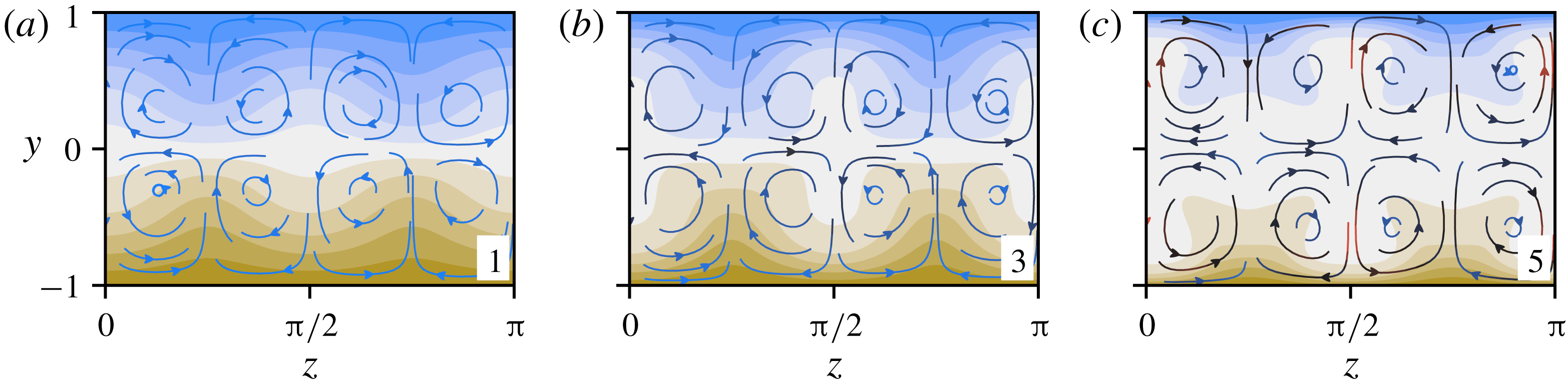
Contour plots of
 $\bar{u}(y,z)$
for
 $Pr=10^{-4}$
solutions at the numbered points indicated on the solid orange figure 4(a) curve. From (a) to (c), the plots correspond to the first (
 $EQ_{7}$
), third (saddle-node) and fifth (
 $EQ_{8}$
) plotted solutions in figure 4(b). Overlaid are
 $(\bar{v},\bar{w})$
-streamlines, coloured with a linear gradient from blue to black to red, according to
 $|(\bar{v},\bar{w})|$
, which lies in the interval
 $[0,0.19)$
.

The qualitative effect of these trends along the solution branches on the streamwise transport is shown in figure 6, which shows the
 $\bar{u}$
field for
 $EQ_{7}$
at
 $\mathit{Ri}_{b}=0$
(a), at the saddle node (b) and
 $EQ_{8}$
at
 $\mathit{Ri}_{b}=0$
(c). This shows that by the end of the lower branch,
 $\hat{u}$
is large enough to cancel the base laminar shear flow solution in some regions (i.e.
 $u=y+\hat{u} =0$
). The overlaid streamlines highlight the underlying roll advection, its increasing significance and the uneven distribution of inflow versus outflow to the walls. However, it is important to note that while streamwise-averaged quantities indicate overall trends, the streamwise dependence observed in figure 1 is present and persists along the solution curves. Specifically, it is not the case that
 $u$
is homogenised throughout the channel interior along the upper branch, even though this is true in a streamwise-averaged sense.
3.2 High Prandtl number (
$Pr\gg 1$
)

Just as in the case of low Prandtl number, solution curves calculated with large
 $Pr$
access higher and higher bulk Richardson numbers as
 $Pr$
increases. However, the mechanism which allows this is quite different, since
 $\hat{\unicode[STIX]{x1D70C}}$
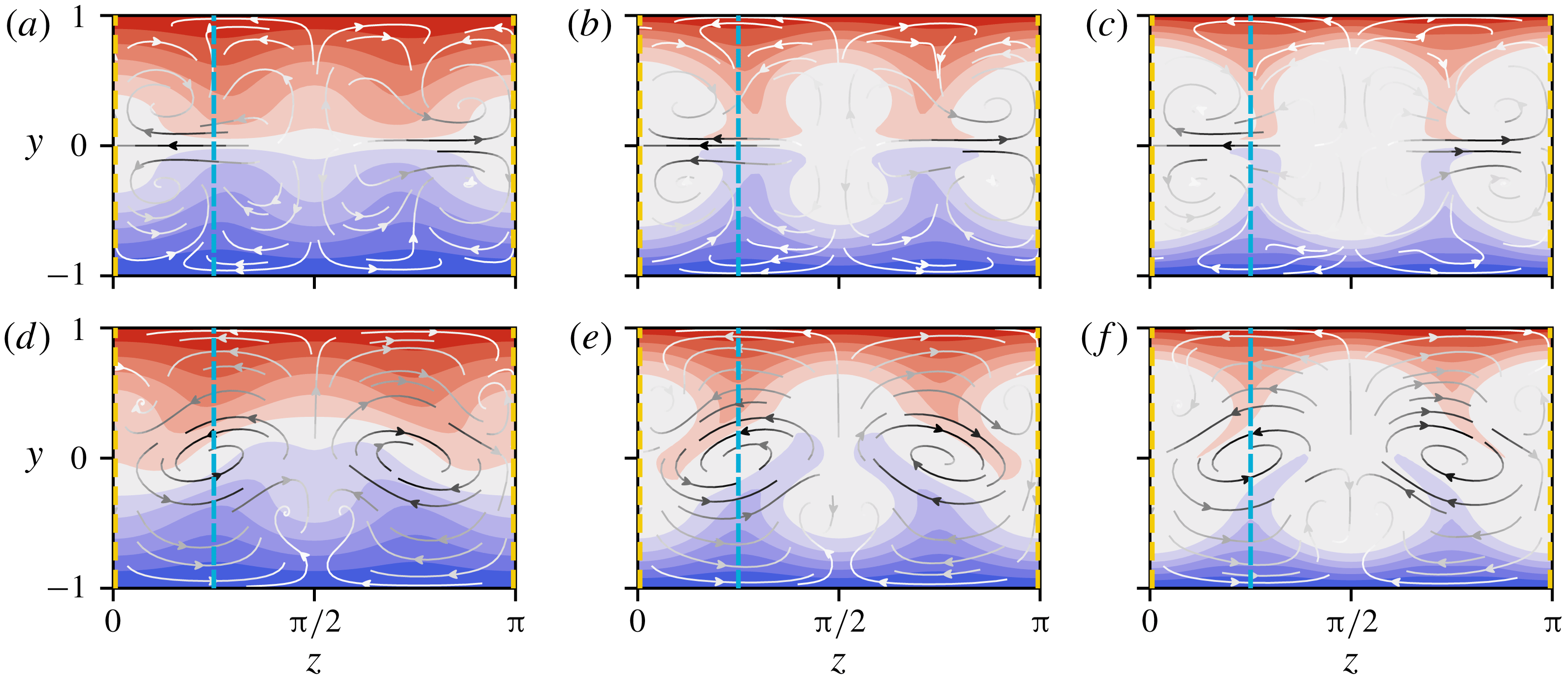
is no longer a weak perturbation of the uniform laminar density profile. In figure 7 we plot contour slices through the
 $yz$
-plane at
 $x=0$
(a–c) and
 $\unicode[STIX]{x03C0}/2$
(d–f) of the full density field
 $\unicode[STIX]{x1D70C}$
for
 $Pr=1$
, 5 and 20. The bulk Richardson number is 0.01 and the velocity field is near that of the (unstratified) lower-branch
 $EQ_{7}$
solution. Starting at
 $Pr=1$
(a,d), the density field for
 $x=0$
is a spanwise-wavy modulation of the laminar base profile. Centred at
 $z=0$
, there is a well-mixed region, where
 $\unicode[STIX]{x1D70C}\approx 0$
, sandwiched between two regions of strong spanwise inflow along the centreline
 $y=0$
. In the
 $\unicode[STIX]{x03C0}/2$
slice, in-plane advection is dominated by vortices centred at
 $(z,y)=(\unicode[STIX]{x03C0}/4,0)$
and
 $(3\unicode[STIX]{x03C0}/4,0)$
, inducing a global spanwise wave. At
 $Pr=5$
(b,e) the spanwise waviness in both
 $x$
slices has become much more exaggerated, with peaks of extremal density advected towards
 $y=0$
and corresponding troughs sent out towards the walls. In between these features, regions of approximately zero density are now well established. By
 $Pr=20$
(c,f), the spanwise-wavy structures have become spanwise localised ‘finger’-like incursions into an otherwise uniformly dense and neutrally buoyant channel interior. Moreover, the regions in the vicinity of the walls have become highly stratified.
Contour plots of
 $\unicode[STIX]{x1D70C}(x,y,z)$
, through
 $x=0$
(a–c) and
 $x=\unicode[STIX]{x03C0}/2$
(d–f) of the
 $EQ_{7}$
state at
 $Pr=1$
, 5 and 20 (left to right) and
 $\mathit{Ri}_{b}=0.01$
. Contours are equally spaced from
 $-1$
(red) to 1 (blue) with a width of
 $2/11$
, ensuring that the middle band (white) is centred at zero. Overlaid are
 $(v,w)$
-streamlines, coloured with a linear gradient from white to black according to the magnitude of
 $(v,w)$
across all six plots, which lies in the interval
 $[0,0.154)$
. The coloured dashed lines through
 $z=0$
and
 $\unicode[STIX]{x03C0}/4$
indicate the locations of the contour slices plotted in figure 8.

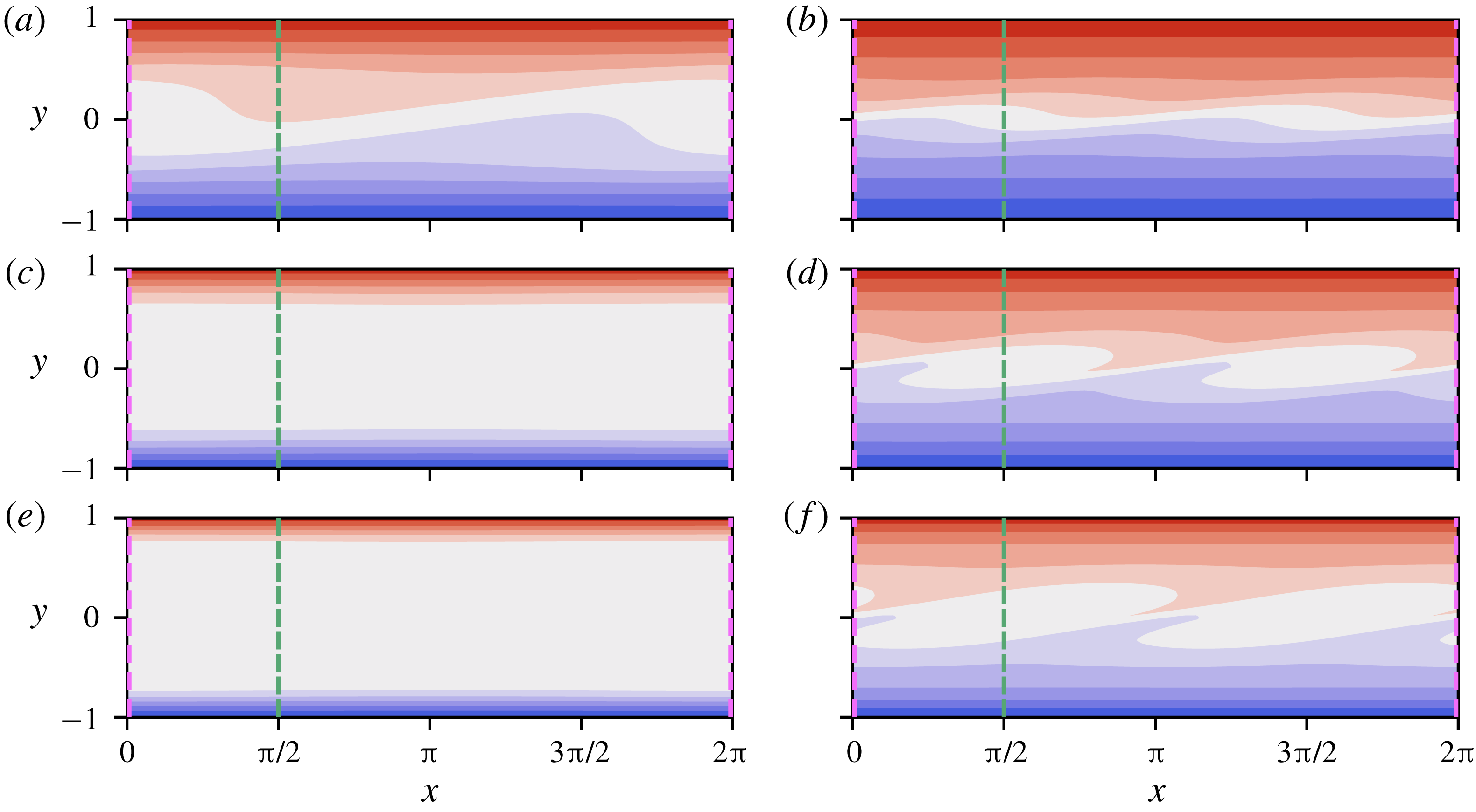
Contour slices through
 $xy$
-planes, of
 $\unicode[STIX]{x1D70C}(x,y,z)$
, at
 $z=0$
(a,c,e) and
 $z=\unicode[STIX]{x03C0}/4$
(b,d,f) of the
 $EQ_{7}$
state at
 $Pr=1$
(a,b), 5 (c,d) and 20 (e,f) and
 $\mathit{Ri}_{b}=0.01$
. The solutions match those depicted in figure 7, as do the contour intervals. The coloured dashed lines at
 $x=0$
and
 $\unicode[STIX]{x03C0}/2$
mark the locations of the contour slices depicted in figure 7.

Figure 8 shows contour slices in the
 $xy$
-plane using the same solutions as figure 7. In this case, the Prandtl number increases moving down each column. Panels (a,c,e) show a slice through
 $z=0$
; we see that the interior in this region is already homogenised by
 $Pr=5$
across the full length of the channel. Panels (b,d,f) show a slice through
 $z=\unicode[STIX]{x03C0}/4$
. Even in this region, by
 $Pr=20$
, the interior appears to be homogenising, despite the aforementioned inflow of density from the walls.
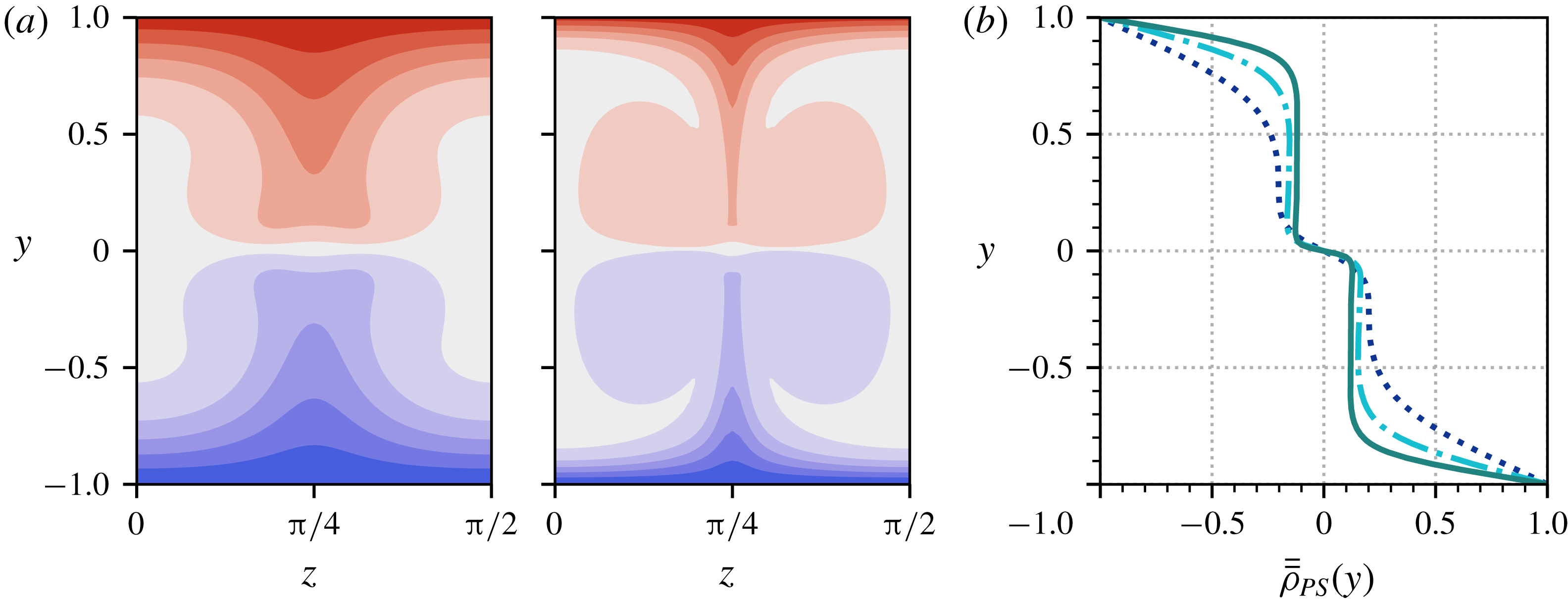
Localisation of stratification as
 $Pr$
increases. The data are from the
 $\mathit{Ri}_{b}=0.01$
solutions depicted in the contour plots of figures 7 and 8. The Prandtl numbers are:
 $Pr=1$
(purple dotted),
 $Pr=5$
(navy dashed),
 $Pr=20$
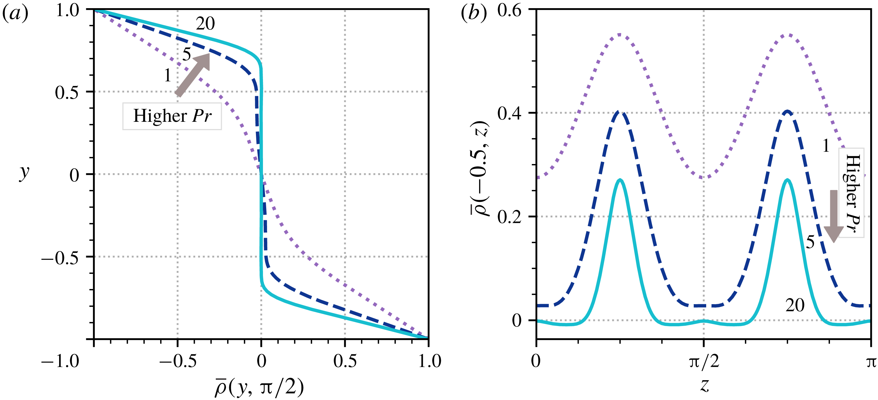
(cyan solid). (a) Vertical profiles of
 $\bar{\unicode[STIX]{x1D70C}}(y,z)$
for fixed
 $z=\unicode[STIX]{x03C0}/2$
, showing the development of boundary layers at the walls. (b) Horizontal slices of
 $\bar{\unicode[STIX]{x1D70C}}(y,z)$
for fixed
 $y=-0.5$
, showing the shrinking width and magnitude of the regions of extremal density uplifted from the boundaries.

At the channel walls, the homogenising density profile must connect to
 $\unicode[STIX]{x1D70C}(x,\pm 1,z)=\mp 1$
. Consequently, as the well-mixed interior region expands, we observe the profile at the walls steepening, developing into separate boundary layers. This is demonstrated in figure 9(a), in which we plot the streamwise-averaged density
 $\bar{\unicode[STIX]{x1D70C}}$
through the line
 $z=\unicode[STIX]{x03C0}/2$
. At
 $Pr=1$
,
 $\bar{\unicode[STIX]{x1D70C}}$
has an almost linear profile. By
 $Pr=20$
, the profile is essentially flat in the interior before becoming highly stratified at the walls. These profiles are reminiscent of turbulent mean temperature profiles of turbulent passively transported scalars simulated by Papavassiliou & Hanratty (Reference Papavassiliou and Hanratty1997), of fully stratified turbulence simulations (Zhou, Taylor & Caulfield Reference Zhou, Taylor and Caulfield2017a
) and of strongly stratified layers observed in geophysical flows (Turner Reference Turner1973). See § 4 for further discussion.
Simultaneously, the finger-like incursions, or ‘density fingers’, seen in figure 7 start to diminish as the channel becomes increasingly well mixed. Figure 9(b) shows horizontal slices of
 $\bar{\unicode[STIX]{x1D70C}}$
at
 $y=-0.5$
. We see that these structures progressively narrow as
 $Pr$
increases. Moreover, from
 $Pr=5$
to
 $Pr=20$
their ‘height’ (
 $\max _{z}\bar{\unicode[STIX]{x1D70C}}$
) and ‘prominence’ (
 $\max _{z}\bar{\unicode[STIX]{x1D70C}}-\min _{z}\bar{\unicode[STIX]{x1D70C}}$
) diminishes. These observations are consistent with the emerging homogenisation of the channel interior region through the plane
 $z=\unicode[STIX]{x03C0}/4$
, seen in figure 8.
It is the diminishing length scales described above that make obtaining solutions at high Prandtl number numerically expensive, ultimately forcing us to cut short some of the continuation curves in figure 2, since states demand increasingly high wall-normal and (to a lesser extent) spanwise resolution as
 $Pr$
increases. Accurately converging states in situations where structures become spatially localised is an important future challenge (see also Olvera & Kerswell Reference Olvera and Kerswell2017). In the following section we obtain higher Prandtl numbers by moving to a regime where we need only solve for the density field (see appendix A).
3.2.1 Passive scalar limit (
$\mathit{Ri}_{b}\rightarrow 0$
)

The passive scalar limit,
 $\mathit{Ri}_{b}\rightarrow 0$
, offers key insight into these high-
 $Pr$
solutions, since in this regime the momentum equation (2.1a
) decouples from the density field. We hereafter adopt the notation
 $\unicode[STIX]{x1D70C}_{PS}$
for the density fields in this limit. The uncoupling of momentum from density allows the stratification equation (2.1c
) to be studied independently from the velocity field, which is just that of the unstratified equilibrium state. Numerically, this limit can be accessed simply by setting
 $\mathit{Ri}_{b}=0$
in the non-dimensionalised system, equations (2.1a
)–(2.1c
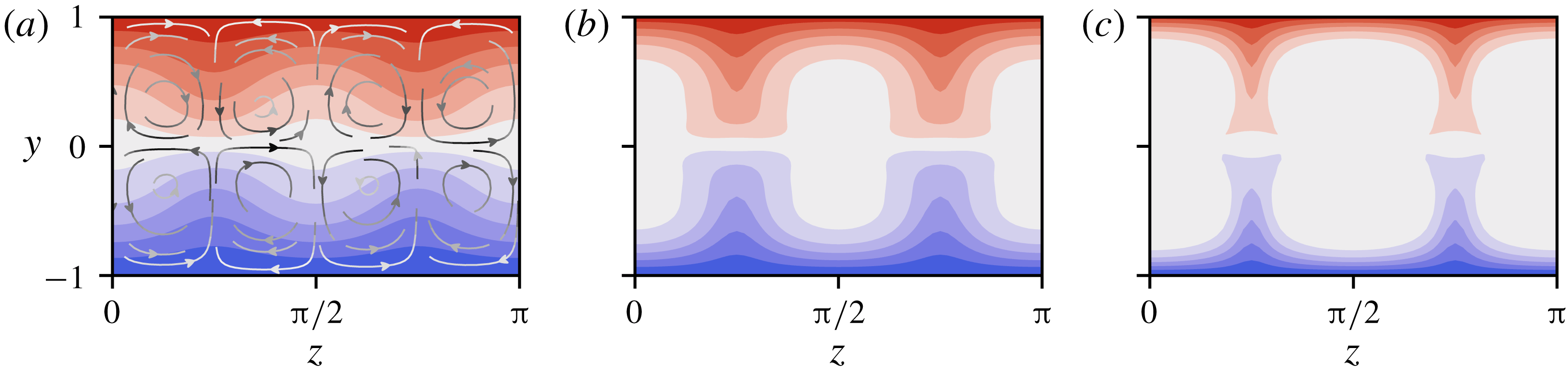
). Figure 10 shows the streamwise-averaged passive scalar density field,
 $\bar{\unicode[STIX]{x1D70C}}_{PS}$
, for
 $EQ_{7}$
at three successively increasing
 $Pr$
. This reveals an underlying structure of stacked rolls and their advective influence on the density field. Much of the character of the density fields described above persists in the
 $\mathit{Ri}_{b}=0$
case. In particular, the spanwise-localised fingers remain, as does the stratified boundary layer, which rapidly diminishes with increasing
 $Pr$
, leaving a largely homogeneous interior.
Contour plots of
 $\bar{\unicode[STIX]{x1D70C}}_{PS}(y,z)$
for increasing
 $Pr$
in the channel cross-section. From (a) to (c)
 $Pr=1$
,
 $Pr=5$
and
 $Pr=20$
are shown. The contour intervals match those in figure 7. Overlaid on the leftmost plot are streamlines of the
 $(\bar{v},\bar{w})$
-field (which is the same for all three solutions), coloured with a linear gradient from white to black according to the magnitude of
 $(\bar{v},\bar{w})$
, which lies in the interval
 $[0,0.02)$
.

The increasing concentration of
 $\unicode[STIX]{x1D70C}_{PS}$
at the boundaries indicates that high-
 $Pr$
solutions must involve a separation of length scales. Considering a boundary layer of thickness
 $\unicode[STIX]{x1D716}$
at the bottom boundary
 $y=-1$
, we define a scaled vertical coordinate
 $Y:=(y+1)/\unicode[STIX]{x1D716}$
and Taylor expand the leading order (VWI) velocity field across the layer
 $$\begin{eqnarray}\displaystyle & u(x,y,z)=-1+\unicode[STIX]{x1D716}u_{1}(x,z)Y+\cdots \,, & \displaystyle\end{eqnarray}$$
 $$\begin{eqnarray}\displaystyle & v(x,y,z)=\unicode[STIX]{x1D716}^{2}Re^{-1}v_{2}(x,z)Y^{2}+\cdots \,, & \displaystyle\end{eqnarray}$$
 $$\begin{eqnarray}\displaystyle & w(x,y,z)=\unicode[STIX]{x1D716}Re^{-1}w_{1}(x,z)Y+\cdots \,, & \displaystyle\end{eqnarray}$$
 $u+1=v=w=0$
at
 $Y=0$
) and incompressibility (
 $\unicode[STIX]{x2202}v/\unicode[STIX]{x2202}y=0$
at
 $Y=0$
). Since the boundaries are well away from the critical layer at
 $y=0$
, the flow fields (as
 $Re\rightarrow \infty$
) have the form
 $$\begin{eqnarray}\displaystyle & u_{1}(x,z)=\bar{u}_{1}(z)+Re^{-7/6}U_{1}(x,z)+\cdots \,, & \displaystyle\end{eqnarray}$$
 $$\begin{eqnarray}\displaystyle & v_{2}(x,z)=\bar{v}_{2}(z)+Re^{-1/6}V_{2}(x,z)+\cdots \,, & \displaystyle\end{eqnarray}$$
 $$\begin{eqnarray}\displaystyle & w_{1}(x,z)=\bar{w}_{1}(z)+Re^{-1/6}W_{1}(x,z)+\cdots \,. & \displaystyle\end{eqnarray}$$
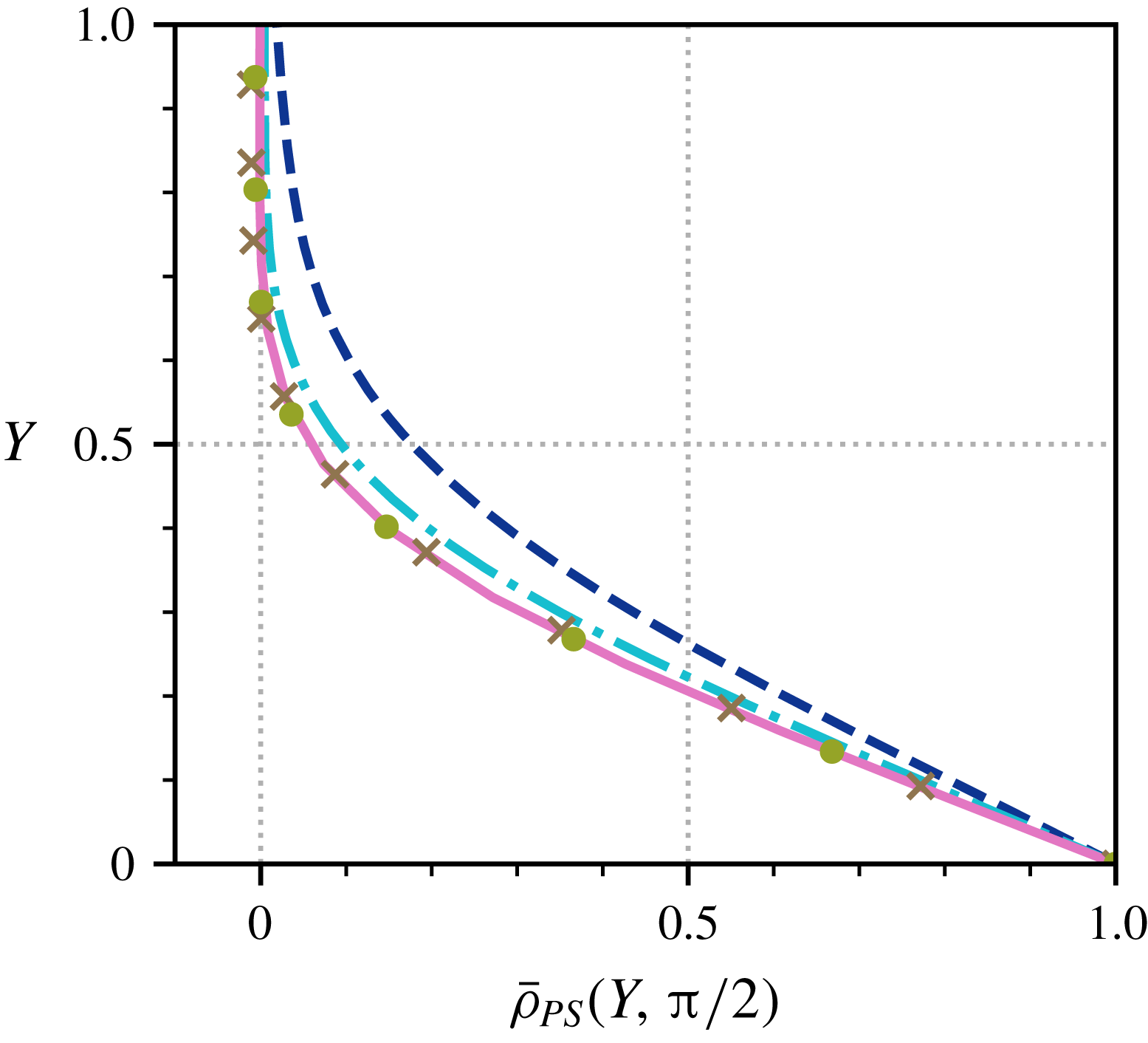
Verification of the boundary layer thickness
 $\unicode[STIX]{x1D716}=Pr^{-1/3}$
. Streamwise-averaged density profiles through
 $z=\unicode[STIX]{x03C0}/2$
are shown, plotted near the wall using boundary layer coordinates
 $Y:=Pr^{1/3}(y+1)$
. The data are from
 $EQ_{7}$
in the passive scalar limit, at
 $Pr=5$
(navy dashed),
 $Pr=20$
(turquoise dash–dot),
 $Pr=100$
(brown crosses),
 $Pr=300$
(olive circles) and
 $Pr=500$
(pink solid). The three highest Prandtl number profiles collapse almost exactly in the rescaled wall-normal coordinates.

It is straightforward to argue that
 $\unicode[STIX]{x1D70C}_{PS}$
must be streamwise invariant at leading order (see appendix B) so that an appropriate expansion for the density field inside the boundary layer is
 $$\begin{eqnarray}\unicode[STIX]{x1D70C}_{PS}(x,Y,z)=\unicode[STIX]{x1D70C}_{0}(Y,z)+\unicode[STIX]{x1D716}\unicode[STIX]{x1D70C}_{1}(x,Y,z)+\cdots \,,\end{eqnarray}$$
where the functions
 $\unicode[STIX]{x1D70C}_{0}$
and
 $\unicode[STIX]{x1D70C}_{1}$
are
 $O(\unicode[STIX]{x1D716}^{0})$
. On substituting (3.5a
)–(3.5c
) into (2.1c
), along with the asymptotic expansion for the density field and dropping all
 $O(\unicode[STIX]{x1D716}^{2})$
terms, we obtain the following leading-order stratification equation:
 $$\begin{eqnarray}-\unicode[STIX]{x1D716}Re\frac{\unicode[STIX]{x2202}\unicode[STIX]{x1D70C}_{1}}{\unicode[STIX]{x2202}x}+\unicode[STIX]{x1D716}v_{2}(x,z)Y^{2}\frac{\unicode[STIX]{x2202}\unicode[STIX]{x1D70C}_{0}}{\unicode[STIX]{x2202}Y}+\unicode[STIX]{x1D716}w_{1}(x,z)Y\frac{\unicode[STIX]{x2202}\unicode[STIX]{x1D70C}_{0}}{\unicode[STIX]{x2202}z}=\frac{1}{\unicode[STIX]{x1D716}^{2}Pr}\frac{\unicode[STIX]{x2202}^{2}\unicode[STIX]{x1D70C}_{0}}{\unicode[STIX]{x2202}Y^{2}}.\end{eqnarray}$$
Balancing advection with diffusion then requires
 $$\begin{eqnarray}\unicode[STIX]{x1D716}=Pr^{-1/3},\end{eqnarray}$$
which is confirmed in figure 11 by plotting
 $\bar{\unicode[STIX]{x1D70C}}_{PS}(Y,z)$
through the line
 $z=\unicode[STIX]{x03C0}/2$
(other values show similar collapse as long as they are not within the finger-like structures). In these coordinates, the density profiles collapse onto each other almost exactly at high
 $Pr$
(
 ${\gtrsim}100$
).
Equation (3.8) splits into a streamwise-independent part which defines
 $\unicode[STIX]{x1D70C}_{0}$
and a streamwise-dependent part which defines
 $\unicode[STIX]{x1D70C}_{1}$
given
 $\unicode[STIX]{x1D70C}_{0}$
as follows:
 $$\begin{eqnarray}\displaystyle & \displaystyle \bar{v}_{2}(z)Y^{2}\frac{\unicode[STIX]{x2202}\unicode[STIX]{x1D70C}_{0}}{\unicode[STIX]{x2202}Y}+\bar{w}_{1}(z)Y\frac{\unicode[STIX]{x2202}\unicode[STIX]{x1D70C}_{0}}{\unicode[STIX]{x2202}z}=\frac{\unicode[STIX]{x2202}^{2}\unicode[STIX]{x1D70C}_{0}}{\unicode[STIX]{x2202}Y^{2}}, & \displaystyle\end{eqnarray}$$
 $$\begin{eqnarray}\displaystyle & \displaystyle Re^{-7/6}V_{2}(x,z)Y^{2}\frac{\unicode[STIX]{x2202}\unicode[STIX]{x1D70C}_{0}}{\unicode[STIX]{x2202}Y}+Re^{-7/6}W_{1}(x,z)Y\frac{\unicode[STIX]{x2202}\unicode[STIX]{x1D70C}_{0}}{\unicode[STIX]{x2202}z}=\frac{\unicode[STIX]{x2202}\unicode[STIX]{x1D70C}_{1}}{\unicode[STIX]{x2202}x}. & \displaystyle\end{eqnarray}$$
 $\bar{w}_{1}^{\prime }(z)=-2\bar{v}_{2}(z)$
, the leading balance, equation (3.10a
), becomes
 $$\begin{eqnarray}\frac{\unicode[STIX]{x2202}^{2}\unicode[STIX]{x1D70C}_{0}}{\unicode[STIX]{x2202}Y^{2}}+\frac{1}{2}\bar{w}_{1}^{\prime }(z)Y^{2}\frac{\unicode[STIX]{x2202}\unicode[STIX]{x1D70C}_{0}}{\unicode[STIX]{x2202}Y}=\bar{w}_{1}(z)Y\frac{\unicode[STIX]{x2202}\unicode[STIX]{x1D70C}_{0}}{\unicode[STIX]{x2202}z},\end{eqnarray}$$
with the boundary conditions
 $\unicode[STIX]{x1D70C}_{0}(0,z)=1$
and
 $\unicode[STIX]{x1D70C}_{0}(Y,z)\rightarrow 0$
as
 $Y\rightarrow \infty$
to match onto a homogenised interior.
At stagnation points
 $z^{\ast }$
where the spanwise velocity is zero, the right-hand side of (3.11) vanishes and it reduces to an ordinary differential equation for
 $\unicode[STIX]{x1D70C}_{0}$
. A solution of this, which decays as it leaves the boundary layer (
 $Y\rightarrow \infty$
), is
 $$\begin{eqnarray}\unicode[STIX]{x1D70C}_{0}(Y,z^{\ast })=1-\frac{(9|\bar{v}_{2}|)^{1/3}}{\unicode[STIX]{x1D6E4}(1/3)}\int _{0}^{Y}\exp \left(\frac{1}{3}\bar{v}_{2}s^{3}\right)\text{d}s,\end{eqnarray}$$
and only exists if
 $\bar{v}_{2}<0$
, i.e. if there is inflow towards the
 $y=-1$
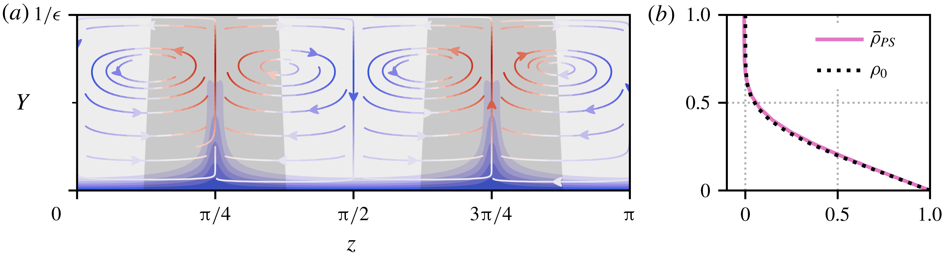
wall. Figure 12(a) shows a contour plot of
 $\bar{\unicode[STIX]{x1D70C}}_{PS}(Y,z)$
at high Prandtl number,
 $Pr=300$
. The density boundary layer is approximately uniform in the spanwise direction where there is inflow into the boundary layer and the asymptotic solution (3.12) matches the numerical solution at the inflow stagnation points: see figure 12(b).
(a) Plot of
 $\bar{\unicode[STIX]{x1D70C}}_{PS}(Y,z)$
in the half-channel
 $0\leqslant Y\leqslant 1/\unicode[STIX]{x1D716}$
, for
 $Pr=300$
, contoured with intervals matching those in figure 7. The streamlines show the streamwise-averaged fluid motion in the
 $(Y,z)$
-plane and are coloured from blue (inflow toward the wall), to white (
 $\bar{v}=0$
), to red (outflow from the wall) according to the value of
 $\bar{v}$
. Regions of outflow are shaded grey. (b) Asymptotic density profile
 $\unicode[STIX]{x1D70C}_{0}(Y,z^{\ast })$
(3.12), (black dotted, computed with
 $\bar{v}_{2}=-36.2$
to
 $3~\text{s.f.}$
), plotted alongside the streamwise-averaged density
 $\bar{\unicode[STIX]{x1D70C}}_{PS}(Y,z^{\ast })$
at
 $Pr=300$
, for the inflow stagnation point at
 $z^{\ast }=\unicode[STIX]{x03C0}/2$
.

Significantly, there is no equivalent solution of the form in (3.12), for an ‘outflow’ stagnation point. This is because these points,
 $z=\unicode[STIX]{x03C0}/4$
and
 $3\unicode[STIX]{x03C0}/4$
, are the focus of boundary layer eruptions (see figure 12
a), where the layer scaling breaks down. These eruptions are the
 $\mathit{Ri}_{b}\rightarrow 0$
manifestation of the fingers seen in figure 9 for
 $\mathit{Ri}_{b}=0.01$
. The situation is clearest at high
 $Re$
where the flow and density field are dominantly streamwise independent. Defining a length scale
 $\unicode[STIX]{x1D6FF}$
for the spanwise width of the fingers, the velocity fields may be Taylor expanded about the outflow stagnation points
 $(y,z)=(-1,z^{\ast })$
as follows:
 $\bar{v}(Y,Z)=\unicode[STIX]{x1D716}^{2}Re^{-1}AY^{2}+O(\unicode[STIX]{x1D716}^{2}\unicode[STIX]{x1D6FF},\unicode[STIX]{x1D716}^{3})$
, and (using incompressibility)
 $\bar{w}(Y,Z)=-2\unicode[STIX]{x1D716}\unicode[STIX]{x1D6FF}Re^{-1}AYZ+O(\unicode[STIX]{x1D716}^{2}\unicode[STIX]{x1D6FF},\unicode[STIX]{x1D716}\unicode[STIX]{x1D6FF}^{2})$
, where
 $Z:=(z-z^{\ast })/\unicode[STIX]{x1D6FF}$
and
 $A$
is an
 $O(Pr^{0})$
constant. Then, instead of (3.8), we have
 $$\begin{eqnarray}\unicode[STIX]{x1D716}AY^{2}\frac{\unicode[STIX]{x2202}\unicode[STIX]{x1D70C}_{0}}{\unicode[STIX]{x2202}Y}-2\unicode[STIX]{x1D716}AYZ\frac{\unicode[STIX]{x2202}\unicode[STIX]{x1D70C}_{0}}{\unicode[STIX]{x2202}Z}=\frac{1}{Pr}\left(\frac{1}{\unicode[STIX]{x1D716}^{2}}\frac{\unicode[STIX]{x2202}^{2}\unicode[STIX]{x1D70C}_{0}}{\unicode[STIX]{x2202}Y^{2}}+\frac{1}{\unicode[STIX]{x1D6FF}^{2}}\frac{\unicode[STIX]{x2202}^{2}\unicode[STIX]{x1D70C}_{0}}{\unicode[STIX]{x2202}Z^{2}}\right).\end{eqnarray}$$
As the flow in the boundary layer approaches an outflow stagnation point, it enters a corner region where the cross-stream diffusion becomes subdominant. (See Childress (Reference Childress1979) and Childress & Gilbert (Reference Childress and Gilbert1995), pp. 135–136, for a discussion of this for an equivalent magnetic field problem, although note that there the velocity boundary conditions used there are stress-free rather than no-slip conditions here.) Therefore, the density field is simply advected by the flow and the leading balance is
 $$\begin{eqnarray}\unicode[STIX]{x1D716}AY^{2}\frac{\unicode[STIX]{x2202}\unicode[STIX]{x1D70C}_{0}}{\unicode[STIX]{x2202}Y}-2\unicode[STIX]{x1D716}AYZ\frac{\unicode[STIX]{x2202}\unicode[STIX]{x1D70C}_{0}}{\unicode[STIX]{x2202}Z}=0.\end{eqnarray}$$
This has a solution of the form
 $\unicode[STIX]{x1D70C}_{0}=\unicode[STIX]{x1D70C}_{0}(\unicode[STIX]{x1D713})$
where
 $\unicode[STIX]{x1D713}:=A(\unicode[STIX]{x1D716}Y)^{2}\unicode[STIX]{x1D6FF}Z$
is a streamfunction.
Consider a streamline starting in the boundary layer where
 $(\unicode[STIX]{x1D716},\unicode[STIX]{x1D6FF})=(Pr^{-1/3},1)$
. Then
 $\unicode[STIX]{x1D713}=O(Pr^{-2/3})$
, requiring
 $\unicode[STIX]{x1D716}$
and
 $\unicode[STIX]{x1D6FF}$
to satisfy the condition
 $$\begin{eqnarray}\unicode[STIX]{x1D716}^{2}\unicode[STIX]{x1D6FF}=Pr^{-2/3}\end{eqnarray}$$
as the streamline negotiates the corner. In the corner itself,
 $\unicode[STIX]{x1D716}=\unicode[STIX]{x1D6FF}$
(this is the scaling of the closest point of approach of the streamline to the stagnation point), so the corner is defined by the scalings
 $$\begin{eqnarray}\unicode[STIX]{x1D716}=\unicode[STIX]{x1D6FF}=Pr^{-2/9}.\end{eqnarray}$$
As the streamline leaves the corner region (with
 $\unicode[STIX]{x1D6FF}$
decreasing) to enter the outer finger region, spanwise diffusion grows to balance advection, so that
 $$\begin{eqnarray}\unicode[STIX]{x1D716}AY^{2}\frac{\unicode[STIX]{x2202}\unicode[STIX]{x1D70C}_{0}}{\unicode[STIX]{x2202}Y}-2\unicode[STIX]{x1D716}AYZ\frac{\unicode[STIX]{x2202}\unicode[STIX]{x1D70C}_{0}}{\unicode[STIX]{x2202}Z}=\frac{1}{Pr\unicode[STIX]{x1D6FF}^{2}}\frac{\unicode[STIX]{x2202}^{2}\unicode[STIX]{x1D70C}_{0}}{\unicode[STIX]{x2202}Z^{2}},\end{eqnarray}$$
which requires
 $$\begin{eqnarray}\unicode[STIX]{x1D716}\unicode[STIX]{x1D6FF}^{2}=Pr^{-1}.\end{eqnarray}$$
Combining the conditions (3.15) and (3.18) leads to outer finger scalings of
 $$\begin{eqnarray}\unicode[STIX]{x1D716}=Pr^{-1/9},\quad \unicode[STIX]{x1D6FF}=Pr^{-4/9}.\end{eqnarray}$$
Significantly, this predicts that the extent of the fingers’ intrusion into the interior will ultimately vanish (albeit slowly) as
 $Pr\rightarrow \infty$
in this
 $\mathit{Ri}_{b}\rightarrow 0$
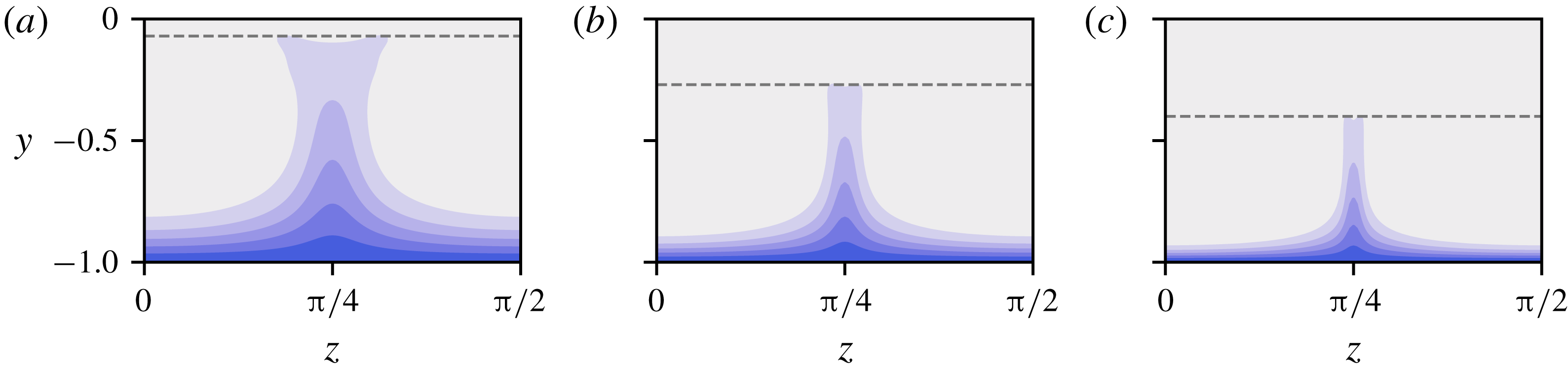
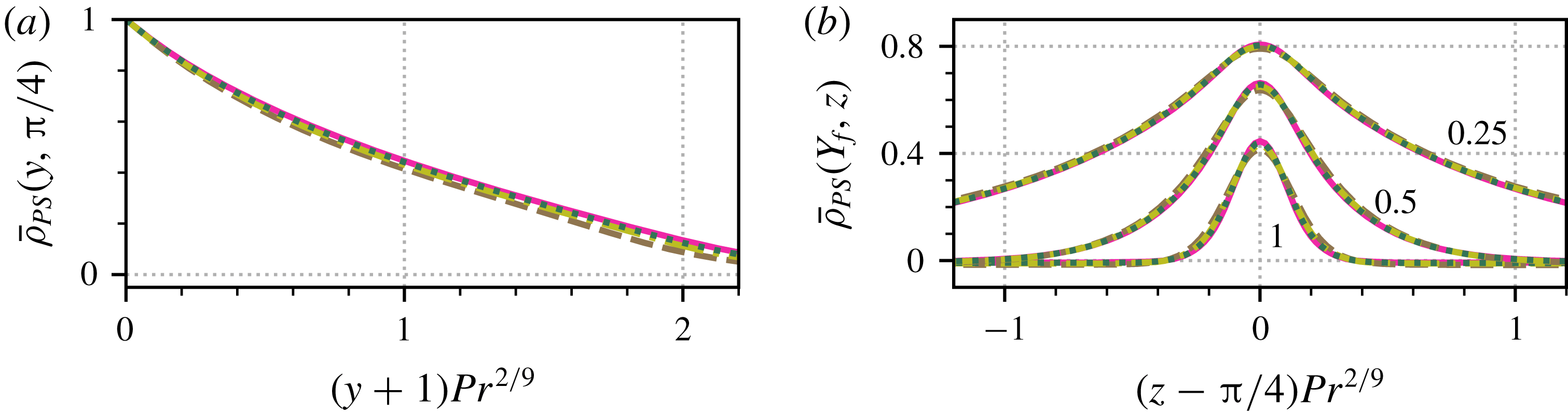
limit, consistent with the contour plots in figure 13. Unfortunately, the Prandtl numbers reached here are not large enough to confirm this small exponent. What is possible is to examine the lower finger profile or corner region. Figure 14(a) shows that streamwise-averaged density profiles through the centreline of the fingers can be collapsed by a rescaled wall-normal coordinate
 $Y_{f}:=(y+1)Pr^{2/9}$
, i.e. the lower parts (corner regions) of the fingers scale like
 $Pr^{-2/9}$
in
 $y$
. Figure 14(b) plots spanwise density profiles of
 $\bar{\unicode[STIX]{x1D70C}}_{PS}$
, across the finger at
 $z=\unicode[STIX]{x03C0}/4$
, at three fixed
 $Y_{f}=0.25$
, 0.5 and 1. On rescaling the spanwise coordinate by
 $Pr^{2/9}$
, the subsequent profiles, ranging from
 $Pr=100$
to 400, collapse well.
Density fingers diminishing with increasing
 $Pr$
in the passive scalar limit. Plotted are contours of
 $\bar{\unicode[STIX]{x1D70C}}_{PS}(y,z)$
at (from a to c)
 $Pr=20$
, 100 and 400. The contour intervals match those in figure 7. We only plot the bottom left quadrant of the full channel – the other parts are dictated by the solution symmetries. The dashed grey lines indicate the approximate height of the finger structures, at
 $y=-0.07$
,
 $-0.27$
and
 $-0.4$
respectively.

The important findings from this passive scalar limit are: (a) a rationale for an
 $O(Pr^{-1/3})$
density boundary layer being formed; (b) the existence of boundary layer eruptions, producing fingers, centred at outflow stagnation points in the boundary layer; and (c) the fact that these eruptions are actually secondary (they diminish with increasing
 $Pr$
) to the primary result that the density gets more and more confined to boundary layers, leaving an homogenised interior as
 $Pr\rightarrow \infty$
. We now examine whether this picture holds more generally for
 $\mathit{Ri}_{b}>0$
equilibria.
Scaling of density fingers at high
 $Pr$
. Both parts plot slices through the same set of solutions in the passive scalar limit, with Prandtl numbers
 $Pr=100$
(brown dashed),
 $Pr=200$
(olive dash–dot),
 $Pr=300$
(dark green dotted) and
 $Pr=400$
(magenta solid). (a) Streamwise-averaged density
 $\bar{\unicode[STIX]{x1D70C}}_{PS}$
through the finger-like structure at
 $z=\unicode[STIX]{x03C0}/4$
, as a function of the rescaled wall-normal coordinate
 $Y_{f}:=(y+1)Pr^{2/9}$
. (b) Streamwise-averaged density profiles in the spanwise coordinate, rescaled in the vicinity of the finger structure at
 $z=\unicode[STIX]{x03C0}/4$
by
 $Pr^{2/9}$
. For each Prandtl number, three slices are plotted at fixed
 $Y_{f}=0.25$
, 0.5 and 1 as indicated.

3.2.2 The case
$\mathit{Ri}_{b}>0$

Sections of the high-
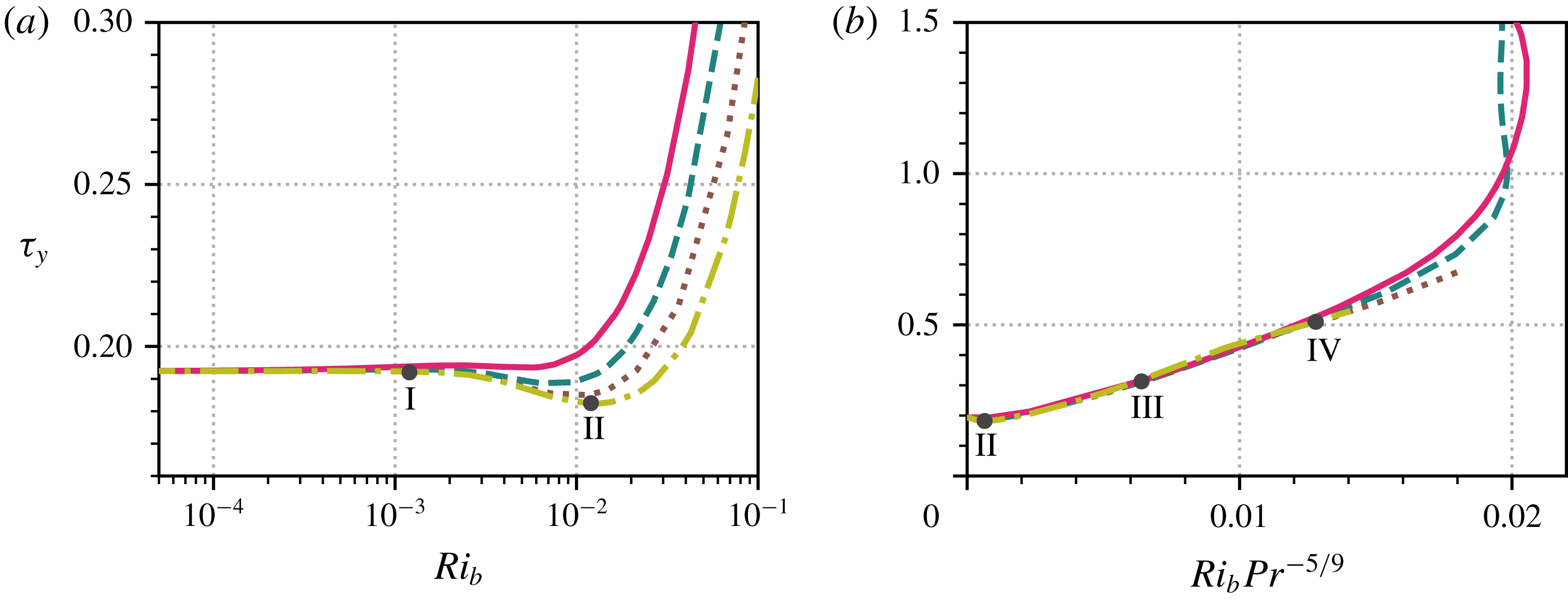
 $Pr$
solution curves from figure 2(b) along the lower branch. Shown are
 $Pr=40$
(magenta solid), 70 (teal dashed), 120 (brown dotted), 200 (olive dash–dot). (a) Low
 $\mathit{Ri}_{b}$
portion with logarithmic horizontal axis. (b) The lower branch plotted with the horizontal axis rescaled by
 $Pr^{-5/9}$
. In both parts, the numerals I–IV indicate the locations of solutions plotted below in figures 16–18.

We now look at how the lower-branch solutions behave as
 $\mathit{Ri}_{b}$
is increased from zero. In figure 15(a), we replot the lower-branch data from figure 2(b) on semi-log axes, for low
 $\mathit{Ri}_{b}$
and
 $Pr\geqslant 40$
(where the boundary layer and finger structures are well developed). As in both the low
 $Pr$
and
 $Pr=O(1)$
(Deguchi Reference Deguchi2017; Olvera & Kerswell Reference Olvera and Kerswell2017) cases, there is necessarily a passive scalar regime where the momentum and stratification equations ((2.1a
) and (2.1c
)) remain effectively uncoupled. This is the approximately horizontal part of the solution branch, from
 $\mathit{Ri}_{b}=0$
to
 $\mathit{Ri}_{b}\approx 10^{-3}$
. The fact that the upper limit of this regime does not display any dependence on
 $Pr$
contrasts with the scaling of
 $\mathit{Ri}_{b}=O(Pr^{-1}Re^{-2})$
for
 $Pr\lesssim O(1)$
(Deguchi Reference Deguchi2017; Olvera & Kerswell Reference Olvera and Kerswell2017, and § 3.1) in which
 $\mathit{Ri}_{b}$
scales inversely with
 $Pr$
. The difference here when
 $Pr\gg 1$
is that the density perturbation
 $\hat{\unicode[STIX]{x1D70C}}$
has to be
 $O(1)$
to homogenise the interior. The buoyancy force is then
 $O(\mathit{Ri}_{b})$
and the streamwise rolls first feel its influence when
 $\mathit{Ri}_{b}=O(Re^{-2})$
. It is worth noting that this argument relies on the fact that the interior is only partly homogenised, otherwise
 $\hat{\unicode[STIX]{x1D70C}}=y$
would precisely cancel out the linear base profile and then the buoyancy force can be exactly balanced by the pressure.
Just beyond
 $\mathit{Ri}_{b}=10^{-3}$
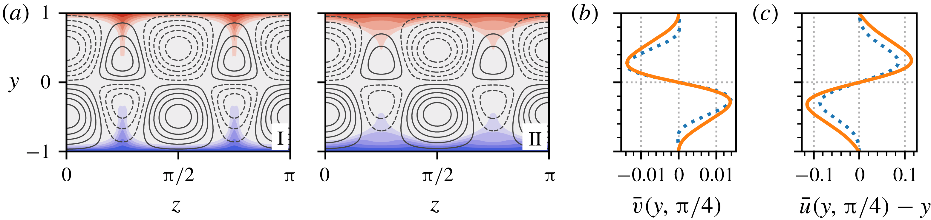
in figure 15(a), the lower-branch solutions all experience a small drop in stress at the walls. The reason for this is encapsulated in figure 16(a), where streamwise-averaged density slices through the
 $yz$
-plane are plotted for the
 $Pr=200$
density field at
 $\mathit{Ri}_{b}=1.2\times 10^{-3}$
(point I, figure 15) and
 $1.2\times 10^{-2}$
(point II, figure 15), with streamwise velocity contours overlaid. Between these two bulk Richardson numbers, the four streaks centred at
 $z=\unicode[STIX]{x03C0}/4$
and
 $3\unicode[STIX]{x03C0}/4$
noticeably weaken and recede from the walls. Increasing
 $\mathit{Ri}_{b}$
penalises the upward motion of dense fluid and likewise the downward motion of less-dense fluid. Consequently, we observe in figure 16(b), that the magnitude of the
 $\bar{v}$
field drops significantly for
 $0.3\lesssim |y|\leqslant 1$
, in the vicinity of the density fingers, leading to the weakening of the streaks there. This is highlighted further in figure 16(c), where we plot streamwise-averaged slices of
 $\hat{u}$
through
 $z=\unicode[STIX]{x03C0}/4$
and see that it drops along the approximate length of the fingers. The density fingers also retreat as
 $\mathit{Ri}_{b}$
increases, since they are no longer vertically advected as strongly. The streaks centred at
 $z=0\equiv \unicode[STIX]{x03C0}$
and
 $\unicode[STIX]{x03C0}/2$
are largely unaffected, since they only experience significant buoyancy forces in the thin boundary layer. Therefore, there is a small reduction in mean wall stress in this regime, caused by the streamwise flow receding from the wall in the finger regions.
Plots demonstrating the stress drop in the high-
 $Pr$
lower branch states. (a) Comparison of
 $EQ_{7}$
at
 $Pr=200$
and
 $\mathit{Ri}_{b}=1.2\times 10^{-3}$
(left) and
 $1.2\times 10^{-2}$
(right), located at points I and II on figure 15(a) respectively. The plots show
 $\bar{\unicode[STIX]{x1D70C}}$
contours in the
 $yz$
-planes, plotted from red (
 $\bar{\unicode[STIX]{x1D70C}}<0$
) to blue (
 $\bar{\unicode[STIX]{x1D70C}}>0$
), using intervals matching those in figure 7. Overlaid in black lines are 10 isolines of the streamwise-averaged
 $\hat{u}$
field, separated by equally spaced intervals between
 $\pm 0.2$
. Dashed lines represent
 $\bar{u}-y<0$
, solid lines
 $\bar{u}-y>0$
. (b) Profiles of
 $\bar{v}$
for the solutions depicted in part (a), through
 $z=\unicode[STIX]{x03C0}/4$
. (c) Corresponding profiles of
 $\bar{u}-y$
, through
 $z=\unicode[STIX]{x03C0}/4$
. In (b,c), solid orange lines are the
 $\mathit{Ri}_{b}=1.2\times 10^{-3}$
state (I) and dashed blue lines are the
 $\mathit{Ri}_{b}=1.2\times 10^{-2}$
state (II).

Following the mean stress drop, there is a marked and sustained rise in
 $\unicode[STIX]{x1D70F}_{y}$
as
 $\mathit{Ri}_{b}$
increases further and states enter a new regime, which covers most of the lower branch. Working on the basis that it is the stratification invading the interior which exerts the leading influence on the ECS, a simple estimate for how
 $\mathit{Ri}_{b}$
varies with
 $Pr$
can be deduced as follows. Assuming the passive scalar finger scalings, the fingers represent an
 $O(1)$
stratification perturbation to the interior in a volume of size
 $O(1)\times O(Pr^{-1/9})\times O(Pr^{-4/9})$
. This is equivalent to an
 $O(Pr^{-5/9})$
stratification over the entire
 $O(1)$
volume which could be expected to influence the wall-normal momentum equation when
 $Re^{-2}\sim \mathit{Ri}_{b}Pr^{-5/9}$
(balancing viscous diffusion with the buoyancy term) or
 $\mathit{Ri}_{b}=O(Pr^{5/9})$
. While the finger scales are by no means guaranteed to persist beyond the weakly stratified regime, figure 15(b) demonstrates a remarkably good collapse of the data.
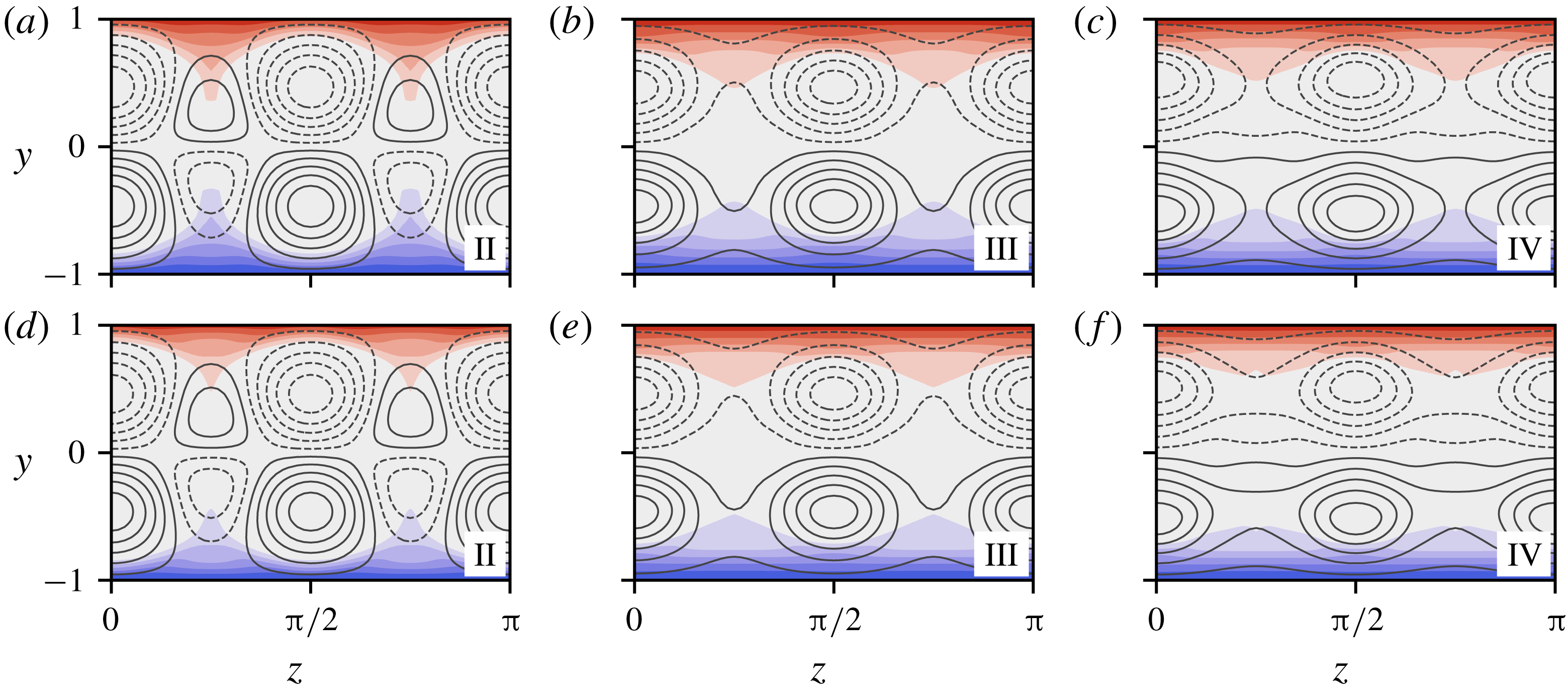
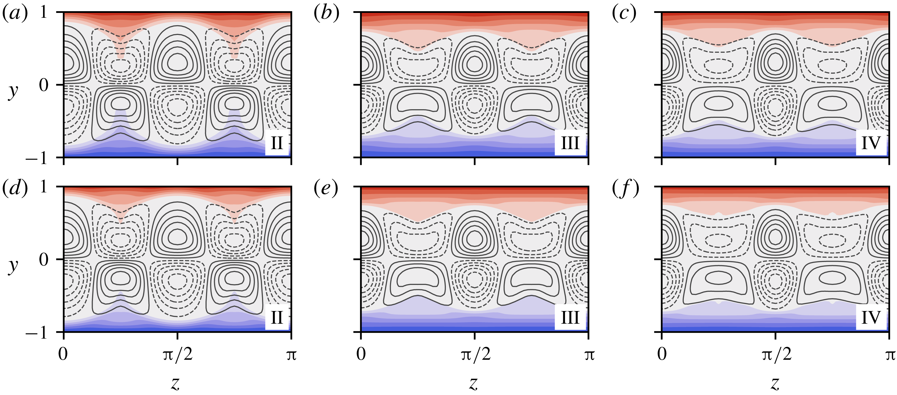
Streamwise-averaged contour plots of
 $EQ_{7}$
at high
 $Pr$
along the (
 $Pr^{-5/9}$
-rescaled) lower branch, at the points II–IV, as indicated in figure 15(b);
 $\mathit{Ri}_{b}Pr^{-5/9}=6.4\times 10^{-4}$
(II),
 $6.4\times 10^{-3}$
(III) and
 $1.28\times 10^{-2}$
(IV), with
 $Pr=70$
(a–c) and 200 (d–f). Contours of
 $\bar{\unicode[STIX]{x1D70C}}(y,z)$
are shown, plotted from red (
 $\bar{\unicode[STIX]{x1D70C}}>0$
) to blue (
 $\bar{\unicode[STIX]{x1D70C}}<0$
); intervals match those in figure 7. Overlaid in black are 10 evenly spaced isolines of the streamwise average of
 $\hat{u}$
, between
 $\pm 0.2$
(II),
 $\pm 0.29$
(III) and
 $\pm 0.37$
(IV). Dashed lines are negative contours and solid lines are positive. For reference, the bulk Richardson numbers for the
 $Pr=70$
data are
 $6.8\times 10^{-3}$
(II),
 $6.8\times 10^{-2}$
(III) and 0.14 (IV). For the
 $Pr=200$
data,
 $\mathit{Ri}_{b}=1.2\times 10^{-2}$
(II), 0.12 (III) and 0.24 (IV).

Figure 17 shows
 $yz$
-contours of the streamwise-averaged streak field
 $\bar{u}-y$
, overlain on
 $\bar{\unicode[STIX]{x1D70C}}$
, for states at three stages along the lower branch, namely the (rescaled) locations labelled on figure 15(b):
 $\mathit{Ri}_{b}Pr^{-5/9}=6.4\times 10^{-4}$
(point II, at the stress drop),
 $6.4\times 10^{-3}$
(point III) and
 $1.28\times 10^{-2}$
(point IV). The similarity between the
 $Pr=70$
and the
 $Pr=200$
fields is immediately striking, with the principal difference only being that the
 $Pr=200$
density field is slightly more homogenised in the interior. In both cases, we see the streak field developing in a similar way to the low
 $Pr$
states (see figure 4); the wall outflow streaks at
 $z=\unicode[STIX]{x03C0}/4$
and
 $3\unicode[STIX]{x03C0}/4$
recede into the interior, become dominated by the inflow streaks at
 $z=0\equiv \unicode[STIX]{x03C0}$
and
 $\unicode[STIX]{x03C0}/2$
(point III), and the streamwise velocity perturbation separates into negative and positive halves (point IV).
Evolution of the
 $\bar{v}$
field for increasing
 $\mathit{Ri}_{b}$
along the high-
 $Pr$
lower branches,
 $Pr=70$
(a–c) and 200 (d–f). Each panel features 10 equally spaced isolines of
 $\bar{v}$
corresponding to the states shown in figure 17, located at points II–IV along the solution branches in figure 15(b). The isolines lie between
 $\pm 0.015$
(II),
 $\pm 0.031$
(III) and
 $\pm 0.05$
(IV), with solid lines indicating
 $\bar{v}>0$
and dashed lines
 $\bar{v}<0$
. Underneath, the
 $\bar{\unicode[STIX]{x1D70C}}(y,z)$
contours (shown in figure 17) are replotted for reference. The bulk Richardson numbers for the
 $Pr=70$
data are
 $6.8\times 10^{-3}$
(II),
 $6.8\times 10^{-2}$
(III), 0.14 (IV) and for the
 $Pr=200$
data:
 $\mathit{Ri}_{b}=1.2\times 10^{-2}$
(II), 0.12 (III) and 0.24 (IV).

The
 $\bar{v}$
fields corresponding to the figure 17 lower-branch states are plotted in figure 18, again with
 $\bar{\unicode[STIX]{x1D70C}}$
underlaid. At the stress drop (II), the
 $\bar{v}$
field covers the full interior, though it is somewhat inhibited in the finger regions. By point III (one third along the lower branch) it has pulled away completely from the highly stratified regions at the walls and remains that way as
 $\mathit{Ri}_{b}$
increases to point IV (two thirds along the lower branch). Meanwhile, the density fingers have smeared out and the stratified layer has thickened, due to readjustment of the advective–diffusive balances there. It is worth noting that the magnitude of
 $\bar{v}$
in the interior has increased substantially. This leads to the growth of the streak fields and the corresponding mean stress increases along the lower branch (see figures 15
b and 17). However, the main message is that faced with increasing stratification at the walls, the
 $\bar{v}$
field isolates itself, pulling in towards the homogenised interior, where
 $\bar{\unicode[STIX]{x1D70C}}\approx 0$
. This appears to be a key mechanism via which the ECS extends the range of
 $\mathit{Ri}_{b}$
at which it can persist before being disrupted. As
 $Pr$
increases for any fixed
 $\mathit{Ri}_{b}$
, the stratified layer recedes further into the walls and the effect of
 $\mathit{Ri}_{b}$
on the structure is less severe. Indeed, our data and associated scaling argument hints that the maximum bulk Richardson number attained by states is
 $\mathit{Ri}_{b}^{m}=O(Pr^{5/9})$
, though it is currently challenging to verify this concretely, given the numerical difficulties inherent in resolving high-
 $Pr$
states and their shrinking length scales.
3.2.3 Other solutions
While Olvera & Kerswell (Reference Olvera and Kerswell2017) isolated
 $EQ_{7}$
and
 $EQ_{8}$
by tracking the edge manifold, many other equilibria exist in plane Couette flow that are dynamically important in the unstratified setting. Since these states, which typically enjoy fewer symmetries than the
 $EQ_{7}/EQ_{8}$
branch, are nevertheless based upon the same SSP/VWI tripartite structure of rolls, streaks and waves, the expectation is that our findings of density homogenisation in the interior with stably stratified boundary layers forming as a consequence at high Prandtl number are generic. To confirm this, we continued solutions
 $EQ_{1}$
–
 $EQ_{11}$
from Gibson et al. (Reference Gibson, Halcrow and Cvitanović2009) to increasing
 $Pr$
in the passive scalar limit (
 $\mathit{Ri}_{b}\rightarrow 0$
) and observed how they change as density transport becomes increasingly convectively dominated.
Streamwise-averaged density fields
 $\bar{\unicode[STIX]{x1D70C}}(y,z)$
for various equilibria in the passive scalar limit. The columns increase in Prandtl number from (a) to (c):
 $Pr=1$
, 10 and 70. The contour intervals match those in figure 7. Streamlines of
 $(\bar{v},\bar{w})$
are shown on (a), coloured with a linear gradient from white to black, according to
 $|(\bar{v},\bar{w})|$
, which has a maximum value of (to 2 significant figures): 0.018 (
 $EQ_{1}$
), 0.098 (
 $EQ_{2}$
), 0.033 (
 $EQ_{3}$
), 0.053 (
 $EQ_{5}$
) and 0.061 (
 $EQ_{10}$
).

Figure 19 shows contours of
 $\bar{\unicode[STIX]{x1D70C}}(y,z)$
for a subset of our converged solutions at
 $Pr=1$
(a), 10 (b) and 70 (c), with overlaid streamlines on column (a) depicting the different roll structures. Just as for
 $EQ_{7}$
in § 3.2.1, each of these new solutions develops a homogenised interior with a corresponding highly stratified boundary layer at the walls. Importantly, each solution features characteristic density fingers, advected into the interior by the rolls, which shrink as
 $Pr$
increases to leave an increasingly homogenised interior. The solutions
 $EQ_{4}$
,
 $EQ_{6}$
,
 $EQ_{9}$
and
 $EQ_{11}$
(not shown) behave similarly.
4 Discussion
In this study, we have computed exact coherent structures in stratified plane Couette flow across a wide range of Prandtl numbers at a fixed Reynolds number
 $Re=400$
. In the two asymptotic limits
 $Pr\ll 1$
and
 $Pr\gg 1$
, states persist to arbitrarily high bulk Richardson numbers, in spite of the stabilising influence of stratification. However, the underlying mechanisms which allow this in each case are quite different.
In the
 $Pr\rightarrow 0$
limit, density transport is diffusion dominated with perturbations from the constant base density gradient being only
 $O(Pr)$
. To leading order, the bulk Richardson number
 $\mathit{Ri}_{b}$
only affects the ECS in the combination
 $\mathit{Ri}_{b}Pr$
with stratification having no noticeable effect on the flow until
 $\mathit{Ri}_{b}=O(Pr^{-1}Re^{-2})$
. Beyond this regime, states continue to follow an
 $O(Pr)$
asymptotic solution curve, reaching a maximum value of
 $\mathit{Ri}_{b}^{m}\approx 0.01/Pr$
at
 $Re=400$
, for the ECS studied in detail here (
 $EQ_{7}$
).
In the
 $Pr\rightarrow \infty$
limit, density transport is advection dominated for any
 $\mathit{Ri}_{b}>0$
, with the interior becoming homogenised as the stratification is confined to boundary layers at the walls (their thickness being
 $O(Pr^{-1/3})$
in the
 $\mathit{Ri}_{b}\rightarrow 0$
limit). The flow and the density stratification are then separated into different parts of the domain with the stratification only starting to influence the velocity field when
 $\mathit{Ri}_{b}=O(Re^{-2})$
independently of
 $Pr$
, which differs from the
 $Pr\lesssim O(1)$
scaling of
 $O(Pr^{-1}Re^{-2})$
(Deguchi Reference Deguchi2017; Olvera & Kerswell Reference Olvera and Kerswell2017). The maximum stratification which can be tolerated by the ECS looks to be
 $\mathit{Ri}_{b}^{m}\sim O(Pr^{5/9})$
at fixed
 $Re$
. Numerically, the situation at large but finite
 $Pr$
and small
 $\mathit{Ri}_{b}$
is complicated by eruptions in the density boundary layers at regions of outflow. These eruptions give rise to fingers, which ultimately vanish to leave a homogenised interior in the limit
 $Pr\rightarrow \infty$
. This behaviour is qualitatively captured in the passive scalar limit (
 $\mathit{Ri}_{b}\rightarrow 0$
) where these fingers have spanwise width
 $O(Pr^{-2/9})$
near the wall, contracting to
 $O(Pr^{-4/9})$
further away and wall-normal length
 $O(Pr^{-1/9})$
.
As discussed in the introduction, a dynamical systems perspective of stratified turbulence imagines a ‘turbulent’ trajectory guided through a complicated phase space by a hierarchy of simple invariant solutions (ECS) and their entangled stable and unstable manifolds. Therefore, it is reasonable to expect that understanding the structure of ECS as a function of the parameters
 $Re$
,
 $Pr$
and
 $\mathit{Ri}_{b}$
may help explain what is seen (maybe fleetingly) in stratified turbulence. Here, we have found simple (laminar) realisations of boundary layers and homogenised regions seen in turbulence with clear scalings emerging, at least for small
 $\mathit{Ri}_{b}$
. For example, the
 $O(Pr^{-1/3})$
boundary layers found here resonate with empirical observations (Kader Reference Kader1981; Schlichting & Gersten Reference Schlichting and Gersten2016) and recent numerical work (Zhou et al.
Reference Zhou, Taylor and Caulfield2017a
) concerning the thickness of the conductive sublayer. Further work is obviously needed to push these to higher
 $\mathit{Ri}_{b}$
and
 $Re$
, but at least this is a start.
Perhaps most noteworthy is the homogenisation seen at high
 $Pr$
, where the shear-driven flow simply clears the stratification out of its way. This limit is costly to simulate at high
 $Re$
since the Péclet number (
 $Pe:=RePr$
) is even larger and hence is little explored. However, hopefully our findings here will help encourage more effort to reach this environmentally relevant limit, since these results clearly highlight the difference between
 $Pr\sim 1$
and
 $Pr$
being large, where a value of 70 (let alone 700 for salt in water) is significant enough to see the difference.
While our results concentrated principally on the highly symmetric
 $EQ_{7}/EQ_{8}$
branch, the high-
 $Pr$
homogenisation of the stratified analogues for the remaining Gibson et al. (Reference Gibson, Halcrow and Cvitanović2009) equilibria demonstrated in § 3.2.3 is an indication that this phenomenon is generic. To establish more fully the relevance of these solutions to observations of real stratified flows, it would be desirable to check whether solutions outside the constraints of our small periodic computational domains behave similarly, especially to see if states with no discrete symmetries can be identified. Moreover, there is the question of whether travelling waves and periodic orbits adapt to increasing
 $Pr$
and
 $\mathit{Ri}_{b}$
in the same way. However, the extremely high resolutions needed to obtain these solutions pushes these computations beyond our reach for now.
Looking ahead, the existence of highly stratified boundary layers found here in the large
 $Pr$
limit begs the question whether stably stratified interior density interfaces could exist for these unstable steady flows. One exploratory computation, taking the
 $EQ_{7}$
solution in the passive scalar limit and increasing
 $Re$
from 400 to
 $10^{5}$
indicates ‘yes’. Figure 20(a) plots contours of the resulting streamwise-averaged density fields and, from
 $Pr=5$
to 70, we see the usual finger structures and boundary layers developing. In this case, however, the top and bottom halves of the channel interior have separated into distinct patches of roughly constant density. In this high-
 $Re$
regime, the ECS converges to a VWI state, becoming streamwise invariant to leading order (see § 2.2). The symmetries of
 $EQ_{7}$
dictate that
 $v(x,0,z)\rightarrow 0$
as
 $Re\rightarrow \infty$
(since the flow becomes increasingly streamwise independent and
 $v(x,0,z)=-v(-x,0,z)$
). Therefore, while density in the top and bottom half-channels can become well mixed as
 $Pr$
increases, there is little exchange between the two. (Note that states such as
 $EQ_{1}$
, whose rolls span the full height of the channel, do not enjoy this property.)
Emergence of internal density interfaces as
 $Pr$
increases at
 $Re=10^{5}$
. (a) Streamwise-normal contour plots of
 $\bar{\unicode[STIX]{x1D70C}}_{PS}(y,z)$
, for
 $Pr=5$
(left) and
 $Pr=70$
(right). Half the channel (
 $0\leqslant z\leqslant \unicode[STIX]{x03C0}/2$
) is shown (the rest being dictated by symmetry). (b) Spanwise- and streamwise-averaged density profiles
 $\bar{\bar{\unicode[STIX]{x1D70C}}}_{PS}:=1/L_{z}\int _{0}^{L_{z}}\bar{\unicode[STIX]{x1D70C}}_{PS}(y,z)\,\text{d}z$
, for
 $Pr=5$
(blue dotted), 20 (turquoise dash-dot) and 70 (teal solid).

Figure 20(b) plots the spanwise average of
 $\bar{\unicode[STIX]{x1D70C}}_{PS}(y,z)$
against
 $y$
for
 $EQ_{7}$
and reveals a highly stratified region at the midplane. In this passive scalar limit where the velocity field is independent of
 $Pr$
, an advective–diffusive balance sets the thickness of this interface at
 $O(Pr^{-1/2})$
which is borne out by the limited data here, plotted in figure 21(a) up to
 $Pr=300$
. The scaling of the density change across the layer is less clear, though
 $O(Pr^{-3/4})$
seems to capture its dependence for
 $Pr\gtrsim 100$
and taken together, these two scales succeed in collapsing the density profiles at the interface in figure 21(b). Whilst this ultimately implies that the interface vanishes in the
 $Pr\rightarrow \infty$
limit, it is nevertheless finite in the
 $Pr=O(10^{2})$
range most relevant to geophysical phenomena. Clearly more computations need to be done to explore this phenomenon.
Empirical scalings of the high-
 $Re$
(
 $=10^{5}$
), high-
 $Pr$
internal layers plotted in figure 20. (a) Log–log plot showing half the interface thickness
 $\unicode[STIX]{x1D6FF}_{y}$
(blue
 $\times$
) and half the density change
 $\unicode[STIX]{x1D6FF}_{\unicode[STIX]{x1D70C}}$
(orange
 $+$
) between the two well-mixed regions, as a function of
 $Pr$
, ranging from 20 to 300. The two black dashed lines are
 $0.4Pr^{-1/2}$
and
 $3.4Pr^{-3/4}$
. Across all data points, the interface is contained within the region
 ${\mathcal{I}}:=(-0.2,0.2)$
and
 $\unicode[STIX]{x1D70C}_{PS}$
reaches an approximately constant value near the edges of this region. Therefore, the half-thickness
 $\unicode[STIX]{x1D6FF}_{y}/2$
was estimated by
 $\operatorname{argmax}_{y\in {\mathcal{I}}}\bar{\unicode[STIX]{x1D70C}}_{PS}(y,3\unicode[STIX]{x03C0}/8)$
and
 $\unicode[STIX]{x1D6FF}_{\unicode[STIX]{x1D70C}}/2$
was estimated using
 $\bar{\unicode[STIX]{x1D70C}}_{PS}(-0.2,3\unicode[STIX]{x03C0}/8)$
. (b) Streamwise- and spanwise-averaged density profiles
 $\bar{\bar{\unicode[STIX]{x1D70C}}}_{PS}(y)$
, rescaled as indicated, by the observed
 $Pr$
-dependences in part (a). The Prandtl numbers are
 $Pr=70$
(teal dotted), 200 (olive dashed), 250 (red dash-dot) and 300 (dark grey solid).

Acknowledgements
The numerical component of this study was carried out using the computational facilities of the Advanced Computing Research Centre, University of Bristol (http://www.bris.ac.uk/acrc/). J.L. acknowledges the support of an EPSRC Doctoral Prize fellowship under grant no. EP/N509619/1 and the Channelflow 2.0 developers, for assistance with their code. R.R.K. acknowledges the support of EPSRC under grant no. EP/K034529/1.
Appendix A. Numerical code details
The flow fields in our direct steady Boussinesq solver are represented by the real part of the truncated pseudo-spectral expansion
 $$\begin{eqnarray}\mathop{\sum }_{m=-M}^{M}\mathop{\sum }_{n=1}^{N}\mathop{\sum }_{l=-L}^{L}\unicode[STIX]{x1D709}_{n,l,m}F_{n}(y)\text{e}^{\text{i}(m\unicode[STIX]{x1D6FC}x+l\unicode[STIX]{x1D6FD}z)}\end{eqnarray}$$
for
 $(x,y,z)\in [0,L_{x}]\times [-1,1]\times [0,L_{z}]$
, where
 $\unicode[STIX]{x1D6FC}=2\unicode[STIX]{x03C0}/L_{x}$
and
 $\unicode[STIX]{x1D6FD}=\unicode[STIX]{x03C0}/L_{z}$
. The
 $\unicode[STIX]{x1D709}_{n,l,m}$
are unknown complex coefficients and
 $F_{n}:=F_{n}^{(r)}+\text{i}F_{n}^{(i)}$
are basis functions in the wall-normal coordinate chosen to satisfy the boundary conditions. For
 $\unicode[STIX]{x1D709}\in \{\hat{u} ,\hat{v},{\hat{w}},\hat{\unicode[STIX]{x1D70C}}\}$
, we have
 $\unicode[STIX]{x1D709}(\pm 1)=0$
and use
 $$\begin{eqnarray}F_{n}^{(r)}=T_{2n+1}-T_{2n-1},\quad F_{n}^{(i)}=T_{2n}-T_{2n-2},\end{eqnarray}$$
where
 $T_{n}$
denotes the
 $n$
th Chebyshev polynomial; for the pressure field we use
 $$\begin{eqnarray}F_{n}^{(r)}=T_{2n-2},\quad F_{n}^{(i)}=T_{2n-1}.\end{eqnarray}$$
We save memory and computation time by omitting coefficients that are fixed by the symmetries defined in (2.6a
)–(2.6c
). In particular,
 ${\mathcal{S}}$
implies that
 $\unicode[STIX]{x1D709}_{n,l,m}=0$
if
 $m+l$
is odd;
 ${\mathcal{Z}}$
implies that
 $\unicode[STIX]{x1D709}_{n,l,m}=\unicode[STIX]{x1D709}_{n,-l,m}$
for
 $\unicode[STIX]{x1D709}\in \{u,v,p,\unicode[STIX]{x1D70C}\}$
and
 $\unicode[STIX]{x1D709}_{n,l,m}=-\unicode[STIX]{x1D709}_{n,-l,m}$
for
 $\unicode[STIX]{x1D709}=w$
;
 $\unicode[STIX]{x1D6FA}$
, together with our basis choices in (A 2) and (A 3) leads to
 $\unicode[STIX]{x1D709}_{n,l,m}^{}=\unicode[STIX]{x1D709}_{n,l,-m}^{\ast }$
for
 $\unicode[STIX]{x1D709}\in \{u,v,p,\unicode[STIX]{x1D70C}\}$
and
 $\unicode[STIX]{x1D709}_{n,l,m}^{}=-\unicode[STIX]{x1D709}_{n,l,-m}^{\ast }$
for
 $\unicode[STIX]{x1D709}=w$
, where the asterisk denotes complex conjugation. These relations reduce the number of Fourier modes required from
 $(2M+1)(2L+1)\approx 4ML$
to
 $\lfloor {\textstyle \frac{1}{2}}((M+1)(L+1)+1)\rfloor \approx ML/2$
.
Equilibria are converged by inverting the steady form of (2.1a
)–(2.1c
) for each Fourier mode at the Chebyshev collocation points
 $y_{j}$
, defined by
 $$\begin{eqnarray}-1<y_{j}:=\cos \left[\frac{\unicode[STIX]{x03C0}(2(j+N)-1)}{4N}\right]<0,\quad j=1,\ldots ,N.\end{eqnarray}$$
Note that the remaining half-channel,
 $0\leqslant y\leqslant 1$
, need not be discretised, since it is given by
 $\unicode[STIX]{x1D6FA}$
.
Solution branches were numerically refined until increasing
 $M$
,
 $N$
or
 $L$
no longer noticeably affected
 $\unicode[STIX]{x1D70F}_{y}$
. Individual states plotted for analysis were typically refined further to ensure that the density field was well resolved. Typical resolutions were
 $(M,N,L)=(12,40,12)$
in the low-
 $Pr$
case (see § 3.1) and up to a maximum of
 $(12,90,38)$
or
 $(10,120,30)$
for high-
 $Pr$
states analysed in § 3.2. In the passive scalar limit
 $\mathit{Ri}_{b}\rightarrow 0$
, the velocity and pressure fields are independent of density. Consequently, we need only solve (2.1c
) subject to fixed
 $u$
,
 $v$
and
 $w$
fields, achieving higher resolution in
 $\unicode[STIX]{x1D70C}$
as a result. This method was to verify the structure scalings derived in § 3.2.1 and to compute the high-
 $Re$
states discussed in § 4, reaching resolutions for the density field of up to
 $(18,140,60)$
and
 $(4,650,68)$
respectively. In all cases the system possessed roughly 200 000 degrees of freedom at maximum resolutions, requiring
 ${\approx}400~\text{GB}$
of computer memory to directly invert the linear operator. Each Newton step at the highest resolutions needed roughly 2 h of wall-clock time on a single compute node with 28 Intel Xeon E5-2680 2.4 GHz cores, making continuation at these resolutions expensive. Tracing out the
 $Pr=70$
branch, for example, required about 1 month of wall-clock time.
Details of the Channelflow code used to compute states in § 3.2.3 may be found elsewhere (Gibson et al.
Reference Gibson, Halcrow and Cvitanović2008, Reference Gibson, Reetz, Azimi, Ferraro, Kreilos, Schrobsdorff, Farano, Yesil, Schütz and Culpo2019). This base code was modified to include (2.1c
) in the time stepping routines. The maximum resolution employed was to converge
 $EQ_{3}$
at
 $Pr=70$
and used a discretised box with
 $(N_{x},N_{y},N_{z})=(120,221,189)$
physical points in the
 $x$
,
 $y$
and
 $z$
directions – approximately 6 million degrees of freedom (though this could have been reduced substantially by decoupling velocity and density as for the direct solver). After omitting dealiased modes this corresponds to maximum Fourier wavenumbers of 39 in
 $x$
, 61 in
 $z$
and 110 collocation points in the half-channel
 $y\in (-1,0)$
. Obtaining a fully stratified state with the direct solver at these resolutions would be infeasible due to memory constraints. A Newton step at this resolution required approximately 6 h of wall-clock time.
Appendix B. Streamwise invariance of the high-
$Pr$
boundary layer

A steady passive scalar layer of thickness
 $\unicode[STIX]{x1D716}$
at the wall in (incompressible) plane Couette flow must be streamwise invariant to leading order. To show that this is true we assume the opposite and reach a contradiction. Substituting the asymptotic expansions of (3.5a
)–(3.5c
) into the steady form of (2.1c
) and presuming
 $\unicode[STIX]{x2202}_{x}\unicode[STIX]{x1D70C}_{PS}=O(\unicode[STIX]{x1D716}^{0})$
leads to the dominant balance
 $$\begin{eqnarray}-\frac{\unicode[STIX]{x2202}\unicode[STIX]{x1D70C}_{PS}}{\unicode[STIX]{x2202}x}=\frac{1}{\unicode[STIX]{x1D716}^{2}RePr}\frac{\unicode[STIX]{x2202}^{2}\unicode[STIX]{x1D70C}_{PS}}{\unicode[STIX]{x2202}Y^{2}}.\end{eqnarray}$$
Taking a Fourier transform of (B 1) in
 $x$
yields
 $-\text{i}k_{x}\unicode[STIX]{x1D716}^{2}RePr\tilde{\unicode[STIX]{x1D70C}}_{PS}=\unicode[STIX]{x2202}_{YY}\tilde{\unicode[STIX]{x1D70C}}_{PS}$
for a given streamwise wavenumber
 $k_{x}$
, where
 $\tilde{\unicode[STIX]{x1D70C}}_{PS}(k_{x},Y,z,t)$
is the transformed density field. At any particular
 $z$
, this has the general solution
 $$\begin{eqnarray}\tilde{\unicode[STIX]{x1D70C}}_{PS}(k_{x};Y,z,t)=C_{1}\text{e}^{Y\sqrt{-\text{i}k_{x}\unicode[STIX]{x1D702}}}+C_{2}\text{e}^{-Y\sqrt{-\text{i}k_{x}\unicode[STIX]{x1D702}}},\end{eqnarray}$$
for constants
 $C_{1}$
and
 $C_{2}$
and
 $\unicode[STIX]{x1D702}:=\unicode[STIX]{x1D716}^{2}RePr$
. For the density field not to blow up in the interior,
 $C_{1}=0$
, leaving just
 $C_{2}$
to be determined. Since the density boundary condition at the wall has no streamwise variation,
 $\tilde{\unicode[STIX]{x1D70C}}_{PS}(k_{x};0,z,t)=0$
for any
 $k_{x}\neq 0$
. Consequently,
 $C_{2}$
also has to vanish meaning that
 $\unicode[STIX]{x1D70C}_{PS}$
has no streamwise variation, which is a contradiction.