NOMENCLATURE

b

wing span (m)

c

reference chord length (m)

c(z)

vector of inequality constraints

C _(⋅)

cosine of an angle

$$\tilde{C}_{{D0}} $$

average contribution of control surface deflections to C _D

C _D0, C _Υ0, C _L0

intercept terms in the expression of C _D , C _Υ and C _L , respectively

C _D(⋅), C _Υ(⋅), C _L(⋅)

derivatives of the aerodynamic force coefficients with respect to (⋅)

C _l(⋅), C _m(⋅), C _n(⋅)

derivatives of the aerodynamic moment coefficients with respect to (⋅)

C _Tx , C _Ty

components of the vectored thrust (normalised with QS) along the body x and y axes, respectively

d

distance between the CG and the propeller along the body x-axis (m)

d, b ₀, b _si , b _ci

coefficient vectors in the Fourier series expansion of the flat outputs (i=1,…, M), belonging to ℝ⁶

D, L

aerodynamic drag and lift force in the wind axes (N)

f

force on the aircraft in the body frame, acting at the CG (N)

g

acceleration due to gravity at sea-level, 9.806 m/s²

g

vector field representing the right-hand side of the state-space form of the 6DoF equations of motion

h

smooth vector field

H _R

reference altitude, 20 m

i, j, k

natural numbers

I

mass moment of inertia matrix (kg m²)

l _b , u _b

vector of lower bound and upper bound on z, respectively

${\cal L},{\cal M},{\cal N}$

roll, pitch and yaw moment – aerodynamic moments in the wind axes (N m)

m

mass of the aircraft (kg)

M

number of harmonics in the Fourier series representation of the flat outputs

n

load factor

N

number of points within [0, t _f ] where constraints are imposed during optimisation

m

moment on the aircraft in the body frame, acting about the CG (N m)

${\frak p}$

exponent in the wind model, 0.25

[p q r] ^T

components of the body frame angular velocity along the body axes (rad/s)

Q

dynamic head (N/m²)

ℝ

set of real numbers

S

reference surface area (m²)

S _(⋅)

sine of an angle

S

matrix for transforming from the inertial frame to the body frame

t _f

time of flight (s) [u v w] ^T components of the relative wind velocity along the body axes (m/s)

u

vector of control inputs

V _R

wind speed at reference altitude H _R (m/s)

V _T

aircraft’s total airspeed (m/s)

[W _x W _y W _z ] ^T

components of wind velocity along the inertial axes (m/s)

W _xz

∂W _x /∂z (per second)

[x y z] ^T

co-ordinates of the aircraft’s CG in an inertial frame (m)

(X, Y, Z)

inertial frame axes

(X _b , Y _b , Z _b )

body frame axes

x

vector of state variables

y

vector of flat outputs

y ^(k)

k ^th time derivative of y

z

vector of design variables

2.0 AIRCRAFT MODEL

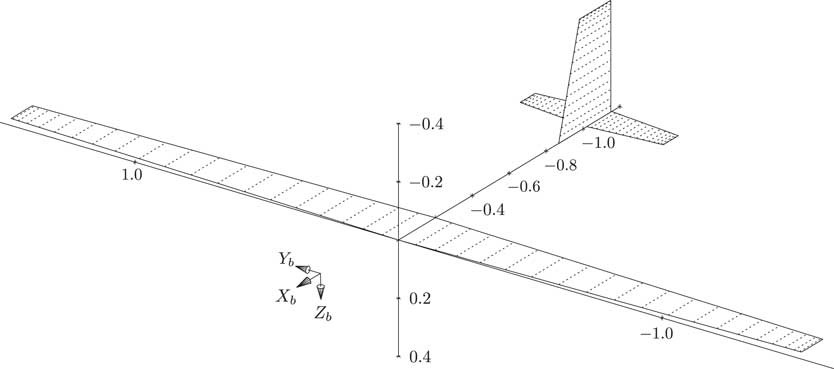
The aircraft model considered in this analysis is a small-scale UAV which is created based on the guidelines followed in Deittert et al.⁽ Reference Deittert, Richards, Toomer and Pipe ^{7 )} and Bower⁽ Reference Bower ^{21 )}. It possesses the attributes of a high aspect-ratio sailplane designed for soaring and has the capacity to vector its thrust in the x–y plane (Fig. 1)

Figure 1

Aircraft geometry generated in AVL

Table 1

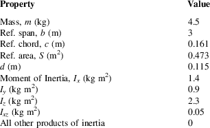
Aircraft parameters

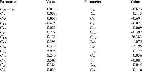
. This model accounts for six control inputs as mentioned previously. The essential parameters of the aircraft are summarised in Table 1. The stability and control derivatives of the aircraft given in Table A1 are used in the computation of aerodynamic coefficients (8). These are estimated using AVL⁽ Reference Drela and Youngren ^{22 )} for a level trimmed flight at a nominal airspeed of 20 m/s. The nominal airspeed is obtained from the solution to the 3DoF trajectory optimisation. It represents the aircraft’s mean airspeed across the duration of the manoeuvre.

3.0 EQUATIONS OF MOTION

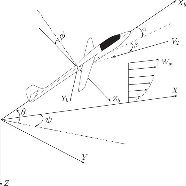
Three co-ordinate frames are required for developing the aircraft’s equations of motion – the Earth-fixed inertial frame, the wind frame and the body-fixed frame. The standard north-east-down co-ordinate axes are used for each of the frames. The body axes, inertial axes and the orientation of the relative wind perceived by the aircraft are depicted in Fig. 2.

Figure 2

Depiction of the various co-ordinate frames.

Dynamic soaring manoeuvres require the presence of wind shear. So a steady wind whose strength varies exponentially with altitude is assumed to blow along the positive x-axis of the inertial frame as shown in (1). The exponential model provides a fairly good representation of the wind speed in the atmospheric boundary layer near the ground and it has been employed in several prior studies of dynamic soaring⁽ Reference Deittert, Richards, Toomer and Pipe ^{7 ,} Reference Liu, Hou, Guo, Yang and Gao ^{23 ,} Reference Sachs and Bussotti ^{24 )}. In (1), V _R is the wind speed at a reference altitude H _R and it denotes the strength of the wind field. During trajectory optimisation, V _R is a design variable while H _R and ${\frak p}$ are constants, 20 m and 0.25, respectively, adopted from Liu et al.⁽ Reference Liu, Hou, Guo, Yang and Gao ^{23 )}:

(1) $$W_{x} {\equals}V_{R} \left( {{{{\minus}z} \over {H_{R} }}} \right)^{{\frak p}} $$

The relationship between the components of the relative wind velocity along the body axes and the aircraft’s velocity in the inertial frame is given by (2). The components of the wind velocity along the body axes are represented by φ (A.3) and the matrix S (A.2) transforms the inertial axes quantities to the body axes:

(2) $$\left[ {\matrix{ {\dot{x}} \hfill \cr {\dot{y}} \hfill \cr {\dot{z}} \hfill \cr } } \right]{\equals}{\bf S}^{T} \left( {\left[ {\matrix{ u \hfill \cr v \hfill \cr w \hfill \cr } } \right]{\plus}{\bf {<bold>&#x03C6;</bold>}} } \right)$$

Rearrangement of the time derivative of (2) yields us (3) and (4), which concern the forces on the body and the rate of change of the components of the relative wind along the body axes:

(3) $$\left[ {\matrix{ {\dot{u}} \hfill \cr {\dot{v}} \hfill \cr {\dot{w}} \hfill \cr } } \right]{\plus}{\bf S}\dot{\bf S}}^{T} \left[ {\matrix{ u \hfill \cr v \hfill \cr w \hfill \cr } } \right]{\equals}{{\bf f} \over m}{\plus}{\bf S}\left[ {\matrix{ 0 \hfill \cr 0 \hfill \cr g \hfill \cr } } \right]{\minus}{\bf S}\left[ {\matrix{ {W_{{xz}} \dot{z}} \hfill \cr 0 \hfill \cr 0 \hfill \cr } } \right]$$

(4) $${\bf f}{\equals}\left[ {\matrix{ {F_{x} } \hfill \cr {F_{y} } \hfill \cr {F_{z} } \hfill \cr } } \right]{\equals}m\left( {\left[ {\matrix{ {\dot{u}} \hfill \cr {\dot{v}} \hfill \cr {\dot{w}} \hfill \cr } } \right]{\plus}\left[ {\matrix{ {wq{\minus}vr} \hfill \cr {ru{\minus}pw} \hfill \cr {pv{\minus}qu} \hfill \cr } } \right]{\minus}g\left[ {\matrix{ {{\minus}S_{{ \rtheta }} } \hfill \cr {C_{{\rtheta }} S_{\rphi } } \hfill \cr {C_{{\rtheta }} C_{\rphi } } \hfill \cr } } \right]{\plus}W_{{xz}} \dot{z}\left[ {\matrix{ {C_{{\rpsi }} C_{{\rtheta }} } \cr {C_{{\rpsi }} S_{{\rtheta }} {S_{\rphi}} {\minus}S_{{\rpsi }} C_{\rphi } } \cr {C_{{\rpsi }} S_{{\rtheta }} C_{\rphi } {\plus}S_{{\rpsi }} {S_{\rphi} }} \cr } } \right]} \right)$$

The relationship between the body frame angular velocity and the rate of change of the Euler angles is given by (5). This, along with the Euler equations of motion defines the rotational dynamics of the aircraft in (6, 7):

(5) $$\left[ {\matrix{ {\dot{\rphi }} \hfill \cr {\hskip1pt\vskip2pt{\dot{\rtheta }}} \hfill \cr {{\dot{\rpsi }}} \hfill \cr } } \right]{\equals}\left[ {\matrix{ 1 \hfill &#x0026; {S_{\rphi } {\rm tan}\rtheta } \hfill &#x0026; {C_{\rphi } {\rm tan}\rtheta } \hfill \cr 0 \hfill &#x0026; {C_{\rphi } } \hfill &#x0026; {{\minus}S_{\rphi } } \hfill \cr 0 \hfill &#x0026; {S_{\rphi } {\rm sec}\rtheta } \hfill &#x0026; {C_{\rphi } {\rm sec}\rtheta } \hfill \cr } } \right]\left[ {\matrix{ p \hfill \cr q \hfill \cr r \hfill \cr } } \right]$$

(6) $${\bf I}\left[ {\matrix{ {\dot{p}} \hfill \cr {\dot{q}} \hfill \cr {\dot{r}} \hfill \cr } } \right]{\plus}\left[ {\matrix{ p \hfill \cr q \hfill \cr r \hfill \cr } } \right]{\times}\left( {{\bf I}\left[ {\matrix{ p \hfill \cr q \hfill \cr r \hfill \cr } } \right]} \right){\equals}{\bf m},\quad {\bf I}{\equals}\left[ {\matrix{ {\,\,\,\,\,I_{x} } \hfill &#x0026; 0 \hfill &#x0026; {{\minus}I_{{xz}} } \hfill \cr \,\,\,\,0 \hfill &#x0026; {I_{y} } \hfill &#x0026; \,\,\,\,0 \hfill \cr {{\minus}I_{{xz}} } \hfill &#x0026; 0 \hfill &#x0026; {\,\,\,\,I_{z} } \hfill \cr } } \right]$$

(7) $${\bf m}{\equals}\left[ {\matrix{ {M_{x} } \hfill \cr {M_{y} } \hfill \cr {M_{z} } \hfill \cr } } \right]{\equals}\left[ {\matrix{ {I_{x} \dot{p}{\minus}I_{{xz}} \dot{r}} \hfill \cr \,\,\,\,\,{I_{y} \dot{q}} \hfill \cr {I_{z} \dot{r}{\minus}I_{{xz}} \dot{p}} \hfill \cr } } \right]{\plus}\left[ {\matrix{ {(I_{z} {\minus}I_{y} )qr{\minus}I_{{xz}} pq} \hfill \cr {(I_{x} {\minus}I_{z} )pr{\plus}(p^{2} {\minus}r^{2} )I_{{xz}} } \hfill \cr {(I_{y} {\minus}I_{x} )pr{\plus}I_{{xz}} qr} \hfill \cr } } \right]$$

The aerodynamic forces and moments defined in the wind axes are estimated using the component build-up approach in (8). The stability and control derivatives for the corresponding force and moment coefficients are used for this purpose:

(8) $$\matrix{ {C_{D} } {{\equals}{D \over {QS}}{\equals}C_{{D0}} {\plus}C_{{D1}} C_{L} {\plus}C_{{D2}} C_{L}^{2} {\plus}C_{{D{\rm \rdelta }_{f} }}\mid\hskip -2pt{\rm \rdelta }_{f}\hskip -3pt\mid\,{\plus}C_{{D{\rm \rdelta }_{a} }} \,\mid\hskip -2pt{\rm \rdelta }_{a} \hskip -3pt\mid\,{\plus}C_{{D{\rm \rdelta }_{e} }} \,\mid\hskip -2pt{\rm \rdelta }_{e} \hskip -3pt\mid\,{\plus}C_{{D{\rm \rdelta }_{r} }} \mid\hskip -2pt{\rm \rdelta }_{r} \hskip -3pt\mid\,} \hfill \cr {C_{{\rm \Upsilon }} } {{\equals}{{\rm \Upsilon } \over {QS}}{\equals}C_{{{\rm \Upsilon \rbeta }}} {\rm \rbeta }{\plus}C_{{{\rm \Upsilon }p}} {{pb} \over {2V_{T} }}{\plus}C_{{{\rm \Upsilon }r}} {{rb} \over {2V_{T} }}{\plus}C_{{{\rm \Upsilon \rdelta }_{a} }} {\rm \rdelta }_{a} {\plus}C_{{{\rm \Upsilon \rdelta }_{r} }} {\rm \rdelta }_{r} } \hfill \cr \hskip 1.5pt{C_{L} } {{\equals}{L \over {QS}}{\equals}C_{{L0}} {\plus}C_{{L{\rm \ralpha }}} {\rm \ralpha }{\plus}C_{{Lq}} {{qc} \over {2V_{T} }}{\plus}C_{{L{\rm \rdelta }_{f} }} {\rm \rdelta }_{f} {\plus}C_{{L{\rm \rdelta }_{e} }} {\rm \rdelta }_{e} } \hfill \cr \hskip 3pt{C_{l} } {{\equals}{{\cal L} \over {QSb}}{\equals}C_{{l{\rm \rbeta }}} {\rm \rbeta }{\plus}C_{{lp}} {{pb} \over {2V_{T} }}{\plus}C_{{lr}} {{rb} \over {2V_{T} }}{\plus}C_{{l{\rm \rdelta }_{a} }} {\rm \rdelta }_{a} {\plus}C_{{l{\rm \rdelta }_{r} }} {\rm \rdelta }_{r} } \hfill \cr {C_{m} } {{\equals}{{\cal M} \over {QSc}}{\equals}C_{{m0}} {\plus}C_{{m{\rm \ralpha }}} {\rm \ralpha }{\plus}C_{{mq}} {{qc} \over {2V_{T} }}{\plus}C_{{m{\rm \rdelta }_{f} }} {\rm \rdelta }_{f} {\plus}C_{{m{\rm \rdelta }_{e} }} {\rm \rdelta }_{e} } \hfill \cr \hskip 1.5pt{C_{n} }{{\equals}{{\cal N} \over {QSb}}{\equals}C_{{n{\rm \rbeta }}} {\rm \rbeta }{\plus}C_{{np}} {{pb} \over {2V_{T} }}{\plus}C_{{nr}} {{rb} \over {2V_{T} }}{\plus}C_{{n{\rm \rdelta }_{a} }} {\rm \rdelta }_{a} {\plus}C_{{n{\rm \rdelta }_{r} }} {\rm \rdelta }_{r} } \hfill \cr } $$

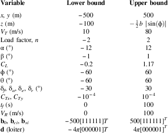
The wind axes are obtained by rotating the body axes through α followed by β. The aerodynamic forces and moments defined in the wind axes can be related to the body axes force f and moment m by appropriate transformation as shown in (9) and (10). It is assumed that the aircraft flies in a co-ordinated fashion i.e. the side-slip β is negligible (C _β≈1 and S _β≈0). This assumption translates to imposing inequality constraints on β during optimisation (Table 2):

(9) $${\bf f}{\equals}\left[ {\matrix{ {F_{x} } \hfill \cr {F_{y} } \hfill \cr {F_{z} } \hfill \cr } } \right]{\equals}QS\left[ {\matrix{ {{\minus}C_{{\rm \ralpha }} C_{D} {\plus}S_{{\rm \ralpha }} C_{L} {\plus}C_{{Tx}} } \cr {C_{{\rm \Upsilon }} {\plus}C_{{Ty}} } \cr {{\minus}S_{{\rm \ralpha }} C_{D} {\minus}C_{{\rm \ralpha }} C_{L} } \cr } } \right]$$

(10) $${\bf m}{\equals}\left[ {\matrix{ {M_{x} } \hfill \cr {M_{y} } \hfill \cr {M_{z} } \hfill \cr } } \right]{\equals}QS\left[ {\matrix{\hfill {bC_{{\rm \ralpha }} C_{l} {\minus}bS_{{\rm \ralpha }} C_{n} } \hfill \cr \,\,\,\,\,\,\,\,\,\,\,\,\,\,\,\,\,\,\,{cC_{m} } \hfill \cr {bS_{{\rm \ralpha }} C_{l} {\plus}bC_{{\rm \ralpha }} C_{n} {\plus}dC_{{Ty}} } \hfill \cr } } \right]$$

Table 2

Constraints

In (9) and (10), C _Tx and C _Ty denote the components of the normalised thrust along the body x- and y-axes, respectively. The propeller is placed at a distance d away from the CG along the body x-axis. This leads to a contribution from C _Ty to the moment along the body z-axis.

The set of 12 differential equations ((2), (3), (5) and (7)) for the 12 states – x, y, z, u, v, w, ϕ, θ, ψ, p, q, r constitute the aircraft’s six-degree-of-freedom (6DoF) equations of motion involving 6 control inputs – δ _f , δ _a , δ _e , δ _r , C _Tx , C _Ty .

4.0 FLATNESS OF 6DoF AIRCRAFT

A dynamical system ${{\dot{\bf x}}} $ =g(x,u) with state vector x∈ℝ ⁱ , input vector u∈ℝ ^j and with a smooth vector field g, is differentially flat⁽ Reference Rigatos ^{25 )} if there exists y∈ℝ ^j of the form

(11) $${\bf y}{\equals}{\bf h}({\bf x},{\rm }{\bf u},{\rm }{\dot{\bf u}},\,\ldots\,,{\rm }{\bf u}^{{(k)}} )$$

such that

(12) $$\eqalignno{ &#x0026; {\bf x}{\equals}{\rm }{\mib{<bold>&#x03B6;</bold> }} ({\bf y},{\rm }{\dot{\bf y}},\,\ldots\,,{\rm }{\bf y}^{{(k{\minus}1)}} ){\,\,\rm and} \cr &#x0026; {\bf u}{\equals}{\rm }{<bold>&#x03BE;</bold>} ({\bf y},{\rm }{\dot{\bf y}},\,\ldots\,,{\rm }{\bf y}^{{(k{\minus}1)}} ,{\rm }{\bf y}^{{(k)}} ) $$

where h, ζ and ξ are smooth vector fields defined as

(13) $$\eqalignno{ &#x0026; {\bf h}\,\colon\,{\rm }{\Bbb R}^{i} {\times}({\Bbb R}^{j} )^{{k{\plus}1}} \to{\Bbb R}^{j} , \cr &#x0026; {<bold>&#x03B6;</bold>} \,\colon\,{\rm }({\Bbb R}^{j} )^{k} \to{\Bbb R}^{i} {\rm \,\,and} \cr &#x0026; {<bold>&#x03BE;</bold>} \,\colon\,({\Bbb R}^{ j} )^{{k{\plus}1}} \to{\Bbb R}^{j} $$

From (12), it is seen that all the states and the control inputs can be expressed in terms of the flat outputs and their time derivatives. In addition, there must not exist any differential relation of the form r(y, ${{\dot{\bf y}}} $ , …, y ^(κ))=0 i.e. the flat outputs y should be differentially independent.

The system of 12 nonlinear differential equations described in the previous section will be shown to be differentially flat. The aircraft’s inertial frame co-ordinates and the body axes Euler angles, (x, y, z, ϕ, θ, ψ), are picked as flat outputs. All the states and the control inputs can be uniquely represented in terms of these flat outputs and their first two derivatives. Furthermore, the flat outputs are solely a function of the states. In such cases, the system is said to be 0-flat. By rearranging (2) and (5), the states (u, v, w, p, q, r) and their first derivatives can be expressed in terms of the flat outputs as shown in (A.5) and (A.6). These are then substituted into (4) and (7) to obtain f and m, respectively. Following this, (8) is plugged into (9) and (10) to obtain the solution for the control inputs. As a consequence of assuming the side-slip to be negligible, the lateral and the longitudinal aerodynamics become decoupled. This means that the solution to δ _f , δ _e and C _Tx can be obtained independently of δ _a , δ _r and C _Ty . The important steps involved are summarised below.

4.1 Solution for δ _f , δ _e , C _Tx

The terms involving the absolute values of the control inputs are dropped from the expression of C _D in (8) in order to make the process of evaluating the control inputs tractable. This inconsistency is accounted for by adding an extra term $$\tilde{C}_{{D0}} $$ , given by (14), to the drag coefficient. It corresponds to the drag incurred due to average control surface deflections during the period of flight. The x and z components of the body axes force f in (9) can be rearranged to yield (15):

(14) $$\tilde{C}_{{D0}} {\equals}C_{{D{\rm \rdelta }_{f} }} \,\mid\hskip -2pt{\rm \rdelta }_{f} \hskip -3pt\mid\,_{{\rm avg.}} {\plus}C_{{D{\rm \rdelta }_{a} }} \,\mid\hskip -2pt{\rm \rdelta }_{a} \hskip -3pt\mid\,_{{\rm avg.}} {\plus}C_{{D{\rm \rdelta }_{e} }} \,\mid\hskip -2pt{\rm \rdelta }_{e} \hskip -3pt\mid\,_{{\rm avg.}} {\plus}C_{{D{\rm \rdelta }_{r} }} \,\mid\hskip -2pt{\rm \rdelta }_{r} \hskip -3pt\mid\,_{{\rm avg.}} $$

(15) $$\eqalignno{ &#x0026; f_{1} {\equals}{{F_{x} } \over {QS}}S_{{\rm \ralpha }} {\minus}{{F_{z} } \over {QS}}C_{{\rm \ralpha }} {\equals}{\rm }C_{L} {\plus}S_{{\rm \ralpha }} C_{{Tx}} \cr &#x0026; f_{2} {\equals}{{F_{x} } \over {QS}}C_{{\rm \ralpha }} {\plus}{{F_{z} } \over {QS}}S_{{\rm \ralpha }} {\equals}{\minus}C_{D} {\plus}C_{{\rm \ralpha }} C_{{Tx}} $$

(16) $$C_{D} {\equals}a_{0} {\plus}a_{1} C_{L} {\plus}a_{2} C_{L}^{2} ,\quad \matrix{ {a_{0} {\equals}C_{{D0}} {\plus}\tilde{C}_{{D0}} } \hfill \cr {a_{1} {\equals}C_{{D1}} } \hfill \cr {a_{2} {\equals}C_{{D2}} } \hfill \cr } $$

A quadratic equation (17) for C _Tx can be obtained from (15) and (16):

(17) $$(a_{2} S_{{\rm \ralpha }}^{2} )C_{{Tx}}^{2} {\plus}({\minus}a_{1} S_{{\rm \ralpha }} {\minus}2a_{2} f_{1} S_{{\rm \ralpha }} {\minus}C_{{\rm \ralpha }} )C_{{Tx}} {\plus}(a_{0} {\plus}a_{1} f_{1} {\plus}a_{2} f_{1}^{2} {\plus}f_{2} ){\equals}0$$

The constants f ₁, f ₂, a ₀, a ₁ and a ₂ are introduced merely for convenience in notation. A simple order of magnitude analysis (A.7–A.10) reveals that only one of the solutions of (17) is physically realisable, hence leaving no room for ambiguity:

(18) $$C_{{Tx}} {\equals}\left( {{{a_{1} S_{{\rm \ralpha }} {\plus}2a_{2} f_{1} S_{{\rm \ralpha }} {\plus}C_{{\rm \ralpha }} } \over {2a_{2} S_{{\rm \ralpha }}^{2} }}} \right){\minus}\sqrt {\left( {{{a_{1} S_{{\rm \ralpha }} {\plus}2a_{2} f_{1} S_{{\rm \ralpha }} {\plus}C_{{\rm \ralpha }} } \over {2a_{2} S_{{\rm \ralpha }}^{2} }}} \right)^{2} {\minus}\left( {{{a_{0} {\plus}a_{1} f_{1} {\plus}a_{2} f_{1}^{2} {\plus}f_{2} } \over {a_{2} S_{{\rm \ralpha }}^{2} }}} \right)} $$

C _L is determined by plugging this solution for C _Tx into (15) while C _m is known from (10). Two linear equations in δ _f and δ _e are then obtained using the expansions for C _L and C _m in (8):

(19) $$\matrix{ \hskip 47pt{{{M_{y} } \over {QSc}}} {\equals} \displaystyle{\mathop{\overbrace{{\left( {C_{{m0}} {\plus}C_{{m{\rm \ralpha }}} {\rm \ralpha }{\plus}C_{{mq}} \left( {{{qc} \over {2V_{T} }}} \right)} \right)}}}^{{\rm }a_{m} {\rm }}{\plus}\mathop{\overbrace{{\left[ {\matrix{ {C_{{m{\rm \rdelta }_{f} }} } \hfill &#x0026; {C_{{m{\rm \rdelta }_{e} }} } \hfill \cr } } \right]}}}^{{\rm }{\bf a}_{m} {\rm }}\left[ {\matrix{ {{\rm \rdelta }_{f} } \hfill \cr {{\rm \rdelta }_{e} } \hfill \cr } } \right]} \hfill \cr {C_{L} {\equals}f_{1} {\minus}S_{{\rm \ralpha }} C_{{Tx}} } {\equals} \displaystyle{\mathop{\overbrace{{\left( {C_{{L0}} {\plus}C_{{L{\rm \ralpha }}} {\rm \ralpha }{\plus}C_{{Lq}} \left( {{{qc} \over {2V_{T} }}} \right)} \right)}}}^{{\rm }a_{L} {\rm }}{\rm }{\plus}\mathop{\overbrace{{\left[ {\matrix{ {C_{{L{\rm \rdelta }_{f} }} } \hfill &#x0026; {C_{{L{\rm \rdelta }_{e} }} } \hfill \cr } } \right]}}}^{{\rm }{\bf a}_{L} {\rm }}\left[ {\matrix{ {{\rm \rdelta }_{f} } \hfill \cr {{\rm \rdelta }_{e} } \hfill \cr } } \right]} \hfill \cr } $$

(20) $$\left[ {\matrix{ \,\,\,\,\,\,\,\,\,{{{M_{y} } \over {QSc}}{\minus}a_{m} } \hfill \cr {f_{1} {\minus}S_{{\rm \ralpha }} C_{{Tx}} {\minus}a_{L} } \hfill \cr } } \right]{\equals}\left[ {\matrix{ {{\bf a}_{m} } \hfill \cr {{\bf a}_{L} } \hfill \cr } } \right]\left[ {\matrix{ {{\rm \rdelta }_{f} } \hfill \cr {{\rm \rdelta }_{e} } \hfill \cr } } \right]$$

4.2 Solution for δ _a , δ _r , C _Ty

The expansions for C _ϒ , C _l and C _n from (8) are substituted into the expressions for F _y , M _x and M _z in (9) and (10). A system of three linear equations in δ _a , δ _r and C _Ty is obtained:

(21) $$\matrix{ \hskip 6.5pt{C_{l} } {\equals} \displaystyle{\mathop{\overbrace{{\left( {C_{{l{\rm \rbeta }}} {\rm \rbeta }{\plus}C_{{lp}} \left( {{{pb} \over {2V_{T} }}} \right){\plus}C_{{lr}} \left( {{{rb} \over {2V_{T} }}} \right)} \right)}}}^{{\rm }a_{l} {\rm }}{\plus}\mathop{\overbrace{{\left[ {\matrix{ {C_{{l{\rm \rdelta }_{a} }} } \hfill &#x0026; {C_{{l{\rm \rdelta }_{r} }} } \hfill &#x0026; 0 \hfill \cr } } \right]}}}^{{\rm }{\bf a}_{{\mib{l}} } {\rm }}\left[ {\matrix{ {{\rm \rdelta }_{a} } \hfill \cr {{\rm \rdelta }_{r} } \hfill \cr {C_{{Ty}} } \hfill \cr } } \right]} \hfill \cr \,\hskip 3pt{C_{n} } {\equals} \displaystyle{\mathop{\overbrace{{\left( {C_{{n{\rm \rbeta }}} {\rm \rbeta }{\plus}C_{{np}} \left( {{{pb} \over {2V_{T} }}} \right){\plus}C_{{nr}} \left( {{{rb} \over {2V_{T} }}} \right)} \right)}}}^{{\rm }a_{n} {\rm }}{\plus}\mathop{\overbrace{{\left[ {\matrix{ {C_{{n{\rm \rdelta }_{a} }} } \hfill &#x0026; {C_{{n{\rm \rdelta }_{r} }} } \hfill &#x0026; 0 \hfill \cr } } \right]}}}^{{\rm }{\bf a}_{{\mib{n}} } {\rm }}\left[ {\matrix{ {{\rm \rdelta }_{a} } \hfill \cr {{\rm \rdelta }_{r} } \hfill \cr {C_{{Ty}} } \hfill \cr } } \right]} \hfill \cr \,\,\,\,{{{F_{y} } \over {QS}}} \hfill {\equals} \hfill \displaystyle{\mathop{\overbrace{{\left( {C_{{{ \Upsilon \rbeta }}} {\rm \rbeta }{\plus}C_{{{\rm \Upsilon }p}} \left( {{{pb} \over {2V_{T} }}} \right){\plus}C_{{{\rm \Upsilon }r}} \left( {{{rb} \over {2V_{T} }}} \right)} \right)}}}^{{\rm }a_{\Upsilon} {\rm }}{\plus}\mathop{\overbrace{{\left[ {\matrix{ {C_{{{\rm \Upsilon \rdelta }_{a} }} } \hfill &#x0026; {C_{{{\rm \Upsilon \rdelta }_{r} }} } \hfill &#x0026; 0 \hfill \cr } } \right]}}}^{{\rm }{\bf a}_{{\Upsilon }} {\rm }}\left[ {\matrix{ {{\rm \rdelta }_{a} } \hfill \cr {{\rm \rdelta }_{r} } \hfill \cr {C_{{Ty}} } \hfill \cr } } \right]} \cr \quad \hskip 4pt \,{\plus}\displaystyle\mathop{\overbrace{{\left[ {\matrix{ 0 \hfill &#x0026; 0 \hfill &#x0026; 1 \hfill \cr } } \right]}}}^{{\rm }{\bf a}_{t} {\rm }}\left[ {\matrix{ {{\rm \rdelta }_{a} } \hfill \cr {{\rm \rdelta }_{r} } \hfill \cr {C_{{Ty}} } \hfill \cr } } \right] \hfill &#x0026; \hfill &#x0026; } } $$

Collecting (21) into a compact form yields us the following equation:

(22) $$\left[ {\matrix{ {{{M_{x} } \over {QSb}}{\minus}\left( {C_{{\rm \ralpha }} a_{l} {\minus}S_{{\rm \ralpha }} a_{n} } \right)} \cr {{{M_{z} } \over {QSb}}{\minus}\left( {S_{{\rm \ralpha }} a_{l} {\plus}C_{{\rm \ralpha }} a_{n} } \right)} \cr {{{F_{y} } \over {QS}}{\minus}a_{{\rm \Upsilon }} } \cr } } \right]{\equals}\left[ {\matrix{ {C_{{\rm \ralpha }} {\bf a}_{l} {\minus}S_{{\rm \ralpha }} {\bf a}_{n} } \cr {S_{{\rm \ralpha }} {\bf a}_{l} {\plus}C_{{\rm \ralpha }} {\bf a}_{n} {\plus}{d \over b}{\bf a}_{t} } \cr {{\bf a}_{{\rm \Upsilon }} {\plus}{\bf a}_{t} } \cr } } \right]\left[ {\matrix{ {{\rm \rdelta }_{a} } \hfill \cr {{\rm \rdelta }_{r} } \hfill \cr {C_{{Ty}} } \hfill \cr } } \right]$$

The flatness of a 6DoF aircraft model with conventional control surfaces and thrust vectoring ability has been brought out. The next section demonstrates how this can be effectively applied to trajectory optimisation for dynamic soaring.

5.0 TRAJECTORY OPTIMISATION FOR DYNAMIC SOARING

The proposed recipe of flatness is applied to 6DoF dynamic soaring trajectory optimisation. As mentioned earlier, dynamic soaring involves the extraction of energy from wind gradient for sustained un-powered flight. Given an aircraft model, it is desirable to know the limiting condition under which it can exhibit dynamic soaring. This corresponds to determining the minimum strength of wind gradient required for achieving the same. In the wind model (2) that is considered in this work, the magnitude of reference wind speed V _R quantifies the strength of wind gradient. The objective of the trajectory optimisation problem is, therefore, the minimisation of V _R . Trajectories where the chosen aircraft can exhibit dynamic soaring with the aid of as low a wind gradient strength as possible are sought.

All the 12 states and the six control inputs have been expressed in terms of the six flat outputs. The dimension of the system is effectively halved and the problem of trajectory optimisation is confined to the space of the flat outputs. The trajectories associated with dynamic soaring necessitate all or most of the states to be periodic. It is then apt to consider a Fourier series-like representation for the flat outputs, y=[x y z ϕ θ ψ] ^T , given by (23), where M is the number of harmonics:

(23) $${\bf y}{\equals}{\bf d}{t \over {t_{f} }}{\plus}{\bf b}_{0} {\plus}\mathop{\sum}\limits_{i{\equals}1}^M {\left\{ {{\bf b}_{{ci}} {\rm \,\,cos}\left( {2{\rm \rpi }i{t \over {t_{f} }}} \right){\plus}{\bf b}_{{si}} {\rm sin}\left( {2{\rm \rpi }i{t \over {t_{f} }}} \right)} \right\}} $$

In (23), t _f represents the time-period of the trajectory and the linear term d is incorporated to model travelling trajectories⁽ Reference Deittert, Richards, Toomer and Pipe ^{7 )}. The elements corresponding to ϕ, θ and z in d are set to zero as these states are necessarily periodic for all kinds of energy-neutral trajectories. The Fourier coefficients of the flat outputs, period of flight t _f and the reference wind speed V _R are treated as the design variables. All of these are collected into the design vector z:

(24) $${\bf z}{\equals}\left[ {\matrix{ {{\bf d}^{T} } \hfill &#x0026; {{\bf b}_{0}^{T} } \hfill &#x0026; {{\bf b}_{{c1}}^{T} } \hfill &#x0026; {{\bf b}_{{s1}}^{T} } \hfill &#x0026; \cdots \hfill &#x0026; {{\bf b}_{{cM}}^{T} } \hfill &#x0026; {{\bf b}_{{sM}}^{T} } \hfill &#x0026; {t_{f} } \hfill &#x0026; {V_{R} } \hfill \cr } } \right]^{T} $$

The optimisation problem is stated as follows:

(25) $$\matrix{ {{\rm minimise}} \hfill &#x0026; {V_{R} } \hfill \cr {{\rm such\ that}} \hfill &#x0026; {{\bf l}_{b} \leq {\bf z}\leq {\bf u}_{b} } \hfill \cr {} \hfill &#x0026; {{\bf c}({\bf z})\leq 0} \hfill \cr {} \hfill &#x0026; {} \hfill \cr } $$

Even though all the states and the controls can be derived from the flat outputs, all combinations for these flat outputs would not translate to physically realisable values for states and controls. For this reason, inequality constraints c(z) are imposed at N uniformly spaced points within the period. In addition to this, upper bound u _b and lower bound l _b are imposed on z. Table 2 lists the constrained variables and their bounds. In order to obtain closed or cross-country trajectories, appropriate constraints are placed on the elements of d corresponding to x and y. The thrust inputs along both the axes are constrained to lie close to zero as the primary motive behind dynamic soaring is to illustrate sustained flight without expending energy from the power plant.

5.1 Initial guess

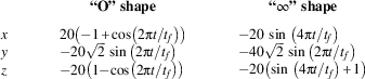
A proper initial guess is necessary for the optimiser to yield a converged solution to the proposed optimisation problem within a reasonable time. It is observed that the solution to the 3DoF flatness-based trajectory optimisation serves as a good initial guess for the proposed 6DoF version. The 3DoF (point mass) version has been implemented by Deittert et al.⁽ Reference Deittert, Richards, Toomer and Pipe ^{7 )}, where the inertial frame co-ordinates of the aircraft (x, y, z) are treated as flat outputs. The coefficients of the Fourier series representation of these outputs serve as design variables. It is noted that the solver consistently fails to converge when an arbitrary initial guess, consisting of pseudo-random values or zeros is provided. On the other hand, provision of initial guesses that capture the approximate shape of the sought dynamic soaring trajectory ensures near-certain convergence of the optimiser. Guess trajectories that mimic the “O” and “∞” shaped dynamic soaring trajectories are shown in Table 3. A Fourier series representation of these is provided as an initial guess to the optimiser. A similar approach was followed in Liu et al.⁽ Reference Liu, Hou, Guo, Yang and Gao ^{23 )}, although the optimisation was performed in time-domain. Cross-country or travelling trajectories can be obtained using the same initial guesses as that for the closed orbits but with constraints placed on the appropriate elements of d. Once the optimal solution for the flat outputs of the 3DoF implementation is obtained, the wind axes orientation angles can be computed by invoking the property of flatness. The details are provided in Deittert et al.⁽ Reference Deittert, Richards, Toomer and Pipe ^{7 )}. These angles serve as a good approximation for the Euler angles of the 6DoF aircraft when α and β are small. The Fourier series approximation for the position time-history and, for these wind axes orientation angles are then provided as initial guess for the 6DoF implementation. Furthermore, the stability and the control derivatives that are required in (8) are estimated for trimmed flight at the mean airspeed observed in the 3DoF solution. This effectively means that the proposed method requires a carefully selected initial guess for the position time-trajectory alone to initiate the flatness-based 3DoF optimisation, whose solution subsequently kick-starts the proposed flatness-based 6DoF optimisation.

Table 3

Initial guess for 3DoF implementation

5.2 Results

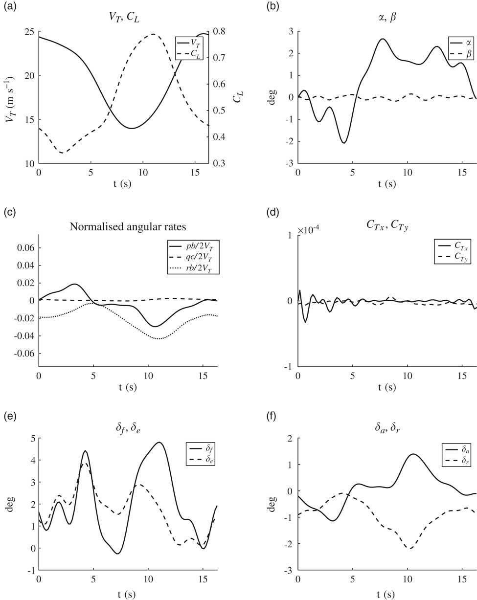
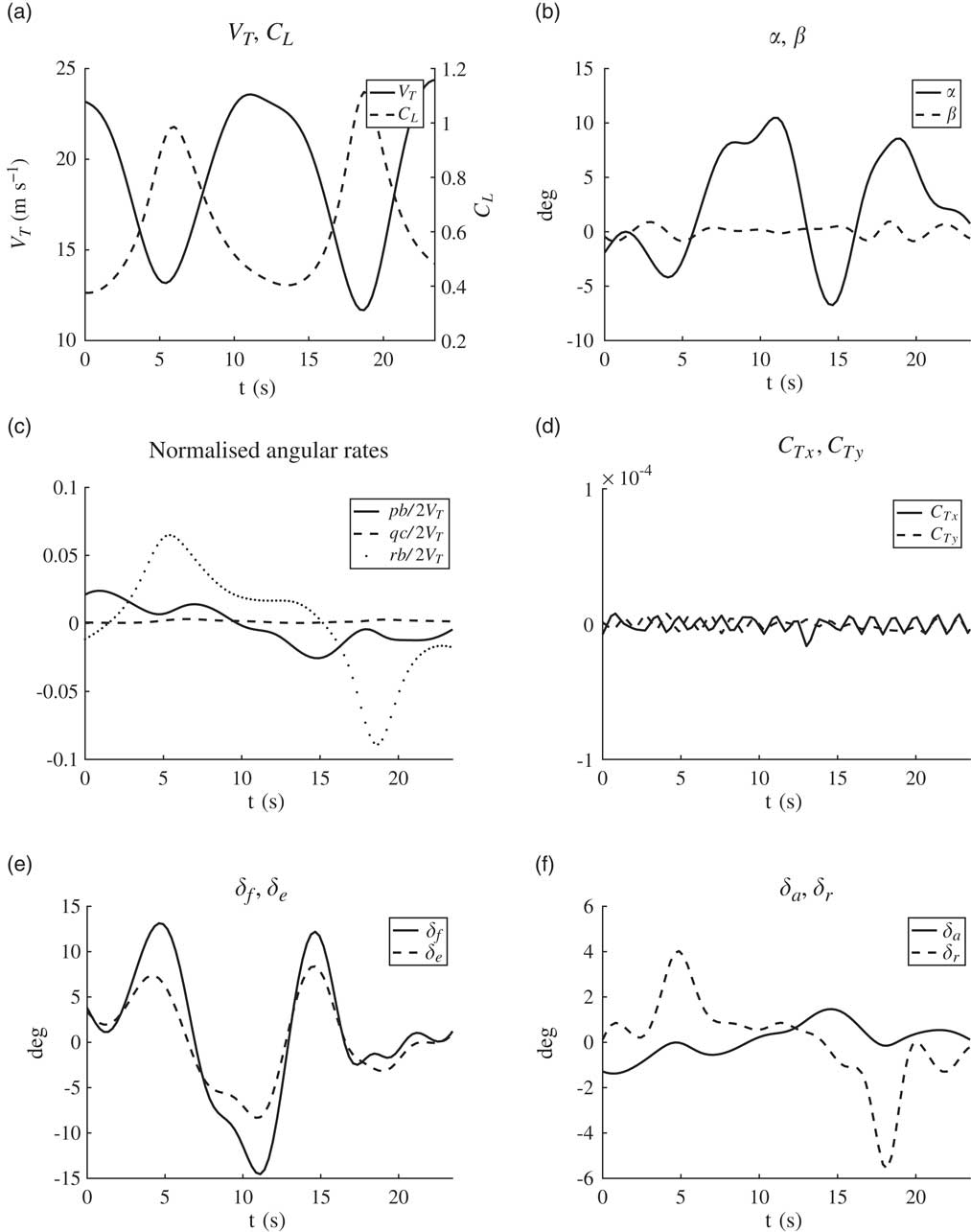
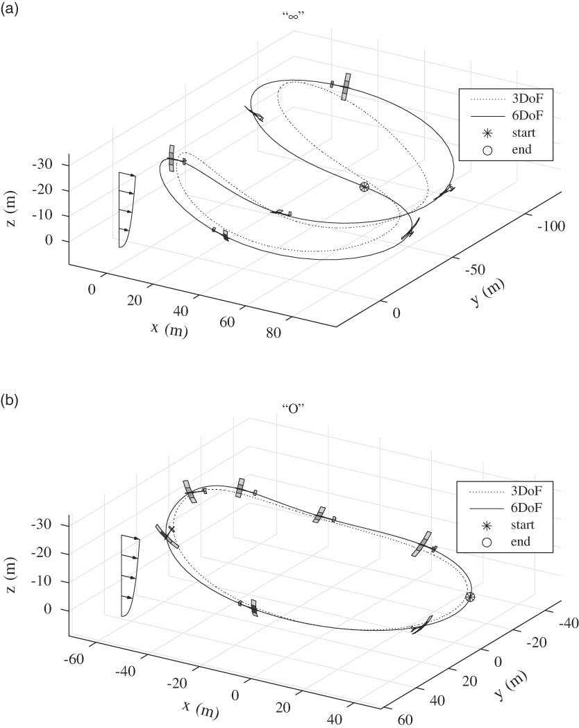
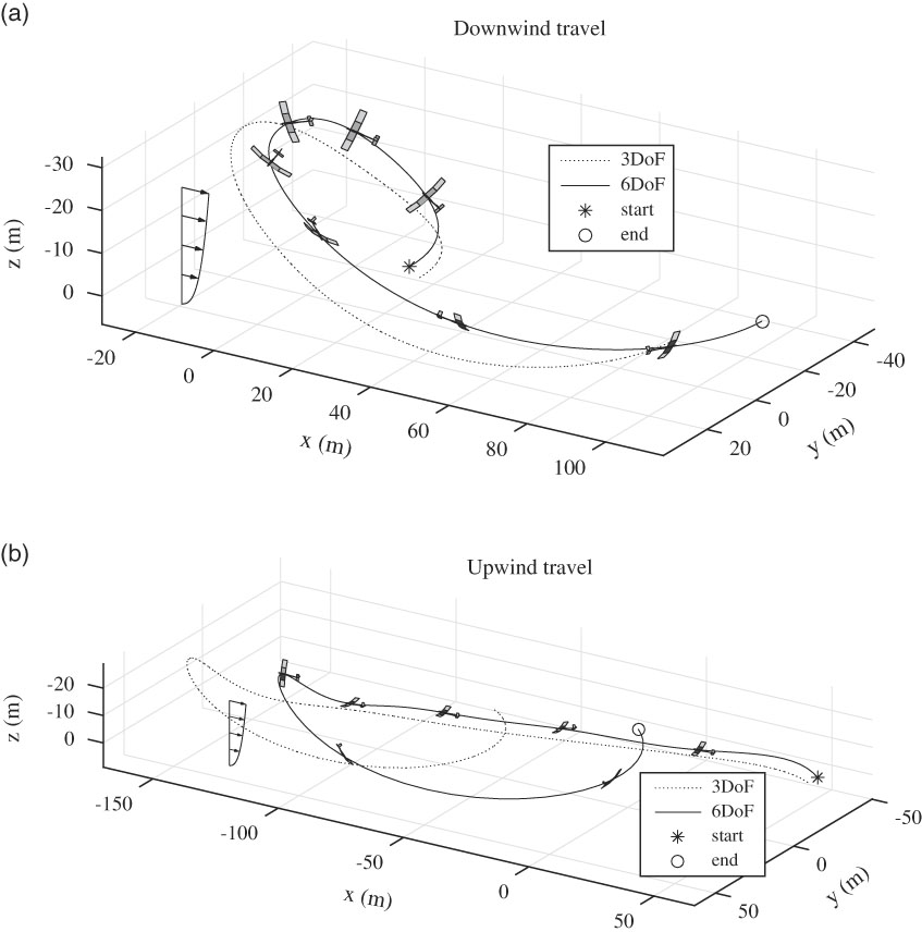
The optimisation problem is solved in MATLAB^® using the nonlinear programming solver, fmincon, and within that the Interior-Point algorithm is selected. The solution for closed and travelling trajectories along with the attitude of the aircraft are illustrated in Figs 6 and 7. The 3DoF trajectories which are provided as initial guesses are also indicated. The optimal wind field strength V _R and the period t _f of the various trajectory solutions are given in Table 4. The observation that the wind strength required for making upwind progress is considerably higher than that required to make the same amount of downwind progress subscribes to the expectations. Among the closed (loiter) trajectories, the “∞” shape requires a smaller wind strength than the “O” shape. Liu et al.⁽ Reference Liu, Hou, Guo, Yang and Gao ^{23 )} have also arrived at the same conclusion and the optimal V _R and t _f calculated by them are very close to that obtained in the present work. The small discrepancy observed is due to the difference in the aircraft models considered. The optimality of the “∞” shape over the “O” shape comes at the cost of large variations in the angle of attack and the control surface deflections (Fig. 4).

Table 4

Optimal parameters

It is seen that the side-slip and the thrust inputs (Figs 3(b) and (d) and 4(b) and (d)) lie within the bounds prescribed in Table 2. Moreover, the assumption of quasi-steady flow inherent in the aerodynamic model is justified as the normalised angular velocity components (Figs 3(c) and 4(c)) are well within the bounds⁽ Reference Drela and Youngren ^{22 )} where the reduced frequency is low.

Figure 3

“O” trajectory

Figure 4

“∞” trajectory

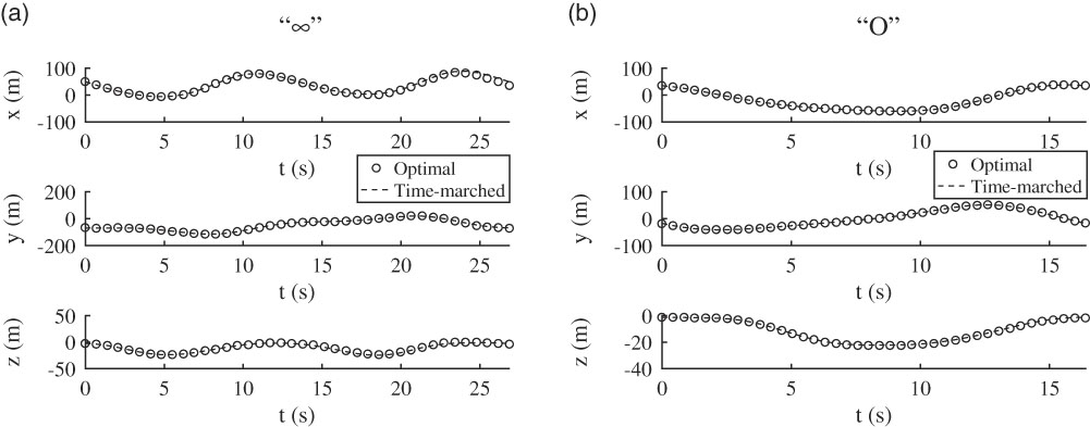
The optimal trajectory solutions from the proposed method are obtained with an approximation (14) introduced to the expression of C _D . Furthermore, since the optimal thrust inputs take very small values within the prescribed bounds, they can be considered to be zero from a practical standpoint. Even after these approximations are accounted for, the optimal solution for the control surface deflections obtained from the proposed flatness-based optimisation is seen to give satisfactory results. The aircraft equations of motion containing the higher fidelity expression for C _D in (8) are time-marched with the optimal control surface deflections and with the thrust inputs set to zero (Fig. 5). It is observed that the error (RMSE) between the time-marched trajectory and that obtained from optimisation does not exceed 0.5 m for “O” shape, and 4 m for “∞” shape. Given the scale of these trajectories, this amounts to less than 5% error. The presence of different time-scales in the aircraft dynamics can be observed in the obtained trajectory solutions (Figs 3 and 4). The contribution of higher harmonics is more evident in the control surface time-histories. The position time-history, on the other hand, does not show rapid variations i.e. the contribution of lower harmonics is dominant. The relative magnitude of the coefficients in their Fourier series representation verifies this observation.

Figure 5

Optimal trajectory and time-marched trajectory

The optimal wind gradient strength reduces when the number of harmonics in the Fourier series expansion of the flat outputs is increased. However, no significant improvement in the optimal solution is noted when more than 12 harmonics are considered.

Visual inspection of the aircraft’s attitude near the top portion of the trajectories, especially in Figs 6(b) and 7(a), seems to indicate a considerably large side-slip. This is in apparent conflict with the computed optimal time-history of β (Figs 3(b) and 4(b)) where the prescribed bounds are not seen to be violated. This apparent discrepancy can be resolved by noting that near the top portion of the trajectory, there is a considerable difference between the aircraft’s airspeed and its inertial frame speed. The large side-slip that is observed in the plots is between the body axes and the inertial frame velocity. On the contrary, the true side-slip β between the body axes and the relative wind vector is indeed small as indicated in Figs 3(b) and4(b).

Figure 6

Closed trajectories

5.2.1 Comparison with the collocation-based optimisation

A direct collocation-based trajectory optimisation is compared with the proposed flatness-based implementation. The former is implemented using Chebyshev pseudospectral method where the set of 12 differential equations are discretized using the Chebyshev differentiation matrix and are posed as nonlinear algebraic equality constraints. These constraints are imposed on a grid of points with Chebyshev spacing within the period of flight. In addition to this, constraints on control rates and those given in Table 2 are also imposed. Chebyshev spacing clusters the grid points towards the extremities and leaves the middle sparse. Due to this, it is observed that at least 35–40 points are required to obtain a satisfactory trajectory solution. The details of the method are provided in Fahroo and Ross⁽ Reference Fahroo and Ross ^{26 )}. The advantage of the flatness-based optimisation is multi-fold. The dimensionality of the direct collocation-based optimisation is significantly higher than that of the proposed flatness-based method. For a trajectory parameterised with 40 points, the former involves 722 design variables while the latter only has 132 when a ten-harmonic representation for the flat outputs is used. 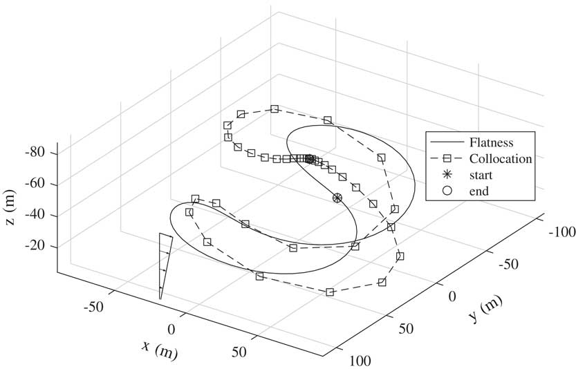The comparison of the trajectory solutions obtained for a linear wind field ( ${\frak p}{\equals}1$ ) from the two approaches is shown in Fig. 8 and Table 5. The codes are run on a machine with 4th generation Intel^® CORE^TM i7 2.6 GHz processor and 8GB of RAM. The flatness-based method has a considerably smaller computational time and yields a continuous solution as compared to the discrete trajectory obtained from the collocation approach. Also, the slightly larger value of V _R from the former should not be construed as the sub-optimality of the flatness-based method over the collocation approach. Such a conclusion cannot be drawn unless a convergence study based on the number of harmonics, collocation points and over a range of initial guesses is undertaken. Second, the control time-histories obtained from the proposed flatness-based implementation are near-optimal but smooth because the flat outputs are parameterised with infinitely differentiable basis functions. On the other hand, the collocation method yields control solutions that possess rapid fluctuations. These fluctuations can be eliminated with the scaling of the control inputs to the same order of magnitude and with the inclusion of constraints on their first derivatives. Another disadvantage that the collocation method suffers from is the inability to converge in a single attempt with the prescribed initial guess (Table 3) when the wind field is changed from linear to exponential. In order to obtain a converged solution for ${\frak p}{\equals}0.25$ , solutions need to be obtained for higher values of ${\frak p}$ (<1) in descending order and used as an initial guess for the optimiser successively. The flatness method, on the contrary, obtains a converged solution in a single attempt without the need for any iterations.

Figure 7

Travelling trajectories

Figure 8

“∞” trajectories from collocation and flatness methods

Table 5

“∞” trajectory from flatness and collocation-based optimisation

At this conjecture, it is apposite to take note of certain salient features and limitations of the proposed recipe of 6DoF aircraft flatness. The provision of six control inputs in an aircraft model, as described in Section 3, is necessary for the proposed recipe to be viable. That being said, for applications involving trajectory generation or tracking, the absent control inputs can be constrained to lie near zero during optimisation. Their contribution, as a consequence, is made negligible, which is equivalent to their absence. This has been demonstrated in the present trajectory optimisation problem where the thrust inputs are constrained (Figs 3(d) and 4(d)). The aerodynamics model is obtained through linearisation about a reference state (steady level cruise). Such a model is valid for trajectories that do not significantly deviate from the reference state. Furthermore, the linear aerodynamics model yields quasi-steady estimate of the forces and moments. In order for the quasi-steady estimate to be reliable, the reduced frequency associated with the flight manoeuvre must be sufficiently small and the angle of attack must not venture into the stall regime. The bounds on the normalised body angular rates suggested by Drela and Youngren⁽ Reference Drela and Youngren ^{22 )} demarcate the region where the quasi-steady assumption is valid. Another crucial assumption that the proposed recipe relies on is that of co-ordinated flight (β≈0). Except in aero-acrobatic manoeuvres, it is usually desirable that the aircraft flies in a co-ordinated fashion. When the side-slip is small, the proposed recipe holds, which as a result allows the aircraft trajectories to be planned in the flat output space. Constraints can be imposed during optimisation such that β lies in a small band near zero, as seen in Figs 3(b) and 4(b).

Aggressive flight manoeuvres are typically costly, in the sense that the airframe is subjected to larger loads and higher fuel consumption is necessitated. In applications involving trajectory generation for reconnaissance or station-keeping missions, it is usually preferable to restrict to benign manoeuvres. The proposed recipe could be advantageous for generating non-aggressive trajectories where α and β are small, and the reduced frequency is sufficiently low. It has been illustrated that the optimal 3DoF solution of a trajectory optimisation problem can be used to construct a good initial guess for the related 6DoF problem, as described in Section 5.1. Furthermore, by using the 3DoF trajectory optimisation solution, an appropriate reference state for linearising the 6DoF aerodynamics can be inferred. The average airspeed over the duration of flight can be determined from the 3DoF solution. Steady level cruise at this mean airspeed would serve as an appropriate reference for linearisation, provided the minimum and the maximum airspeed encountered during the manoeuvre is not significantly different from the mean airspeed. Finally, the proposed recipe has made use of thrust vectoring capability that is confined to the x–y plane. Ideally, it would be more advantageous to vector thrust in all the directions.

Martin’s⁽ Reference Martin ^{14 )} formulation of flatness, in contrast, is applicable for a wider region in the flight envelope as it employs a look-up table spanning operating points for estimating the aerodynamic coefficients. However, the use of a look-up table for trajectory generation or tracking is computationally costly. For this reason, a slightly less accurate low-order functional form for the aircraft’s aerodynamic coefficients (as shown in (8)) is preferable. In addition to this, the advantage of taking the aid of the optimal 3DoF solution to solve a 6DoF trajectory optimisation is absent from Martin’s formulation.