1 Introduction
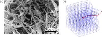
Microorganism motility in a Newtonian fluid is a classical theme in biological fluid mechanics (Lighthill Reference Lighthill1975) and experimental, computational and theoretical studies have elucidated many of its fundamental aspects (Lauga & Powers Reference Lauga and Powers2009). However, microorganisms typically navigate a complex environment composed of a viscous fluid with suspended microstructures such as elastic polymers and filamentous networks. Mammalian sperm must penetrate such heterogeneous networks as they make their way through the female reproductive tract (Fauci & Dillon Reference Fauci and Dillon2006). The arrangement and spacing between mucin fibres of vaginal and cervical mucus vary during the menstrual cycle (Rutllant et al. Reference Rutllant, López-Béjar, Santolaria, Yániz and López-Gatius2002; Rutllant, López-Béjar & López-Gatius Reference Rutllant, López-Béjar and López-Gatius2005). Figure 1(a), from Rutllant et al. (Reference Rutllant, López-Béjar and López-Gatius2005), depicts bovine sperm in a vaginal fluid sample, where the voids in the cross-linked network of filaments are of the order of the size of the sperm head. How do the mechanics and energetics of motility depend upon the network’s microstructure and elastic properties? How does the swimmer’s velocity and orientation fluctuate in response to its interaction with the network? Such questions are also relevant in the development of fabricated micromachines that are driven by magnetic actuation (Tottori et al. Reference Tottori, Zhang, Krawczyk, Franco-Obregon and Nelson2012). For these nanopropellers to be used for biomedical applications, like their natural counterparts, they must be able to move through complex heterogeneous networks (Schamel et al. Reference Schamel, Mark, Gibbs, Miksch, Morozov, Leshansky and Fischer2014).
(a) From Rutllant et al. (Reference Rutllant, López-Béjar and López-Gatius2005), photomicrograph of bovine spermatozoa in a vaginal fluid sample. Scale bar
 $10~{\rm\mu}\text{m}$
. (b) Snapshot of the model flagellar swimmer moving through a viscoelastic network.

The swimming of microorganisms in a non-Newtonian fluid has recently received significant attention. Using a single-phase nonlinear viscoelastic model of the fluid, such as Stokes/Oldroyd-B, it was shown that the swimming velocity of an infinite sheet undergoing sinusoidal oscillations is always impeded by viscoelasticity (Lauga Reference Lauga2007). However, a finite sheet with accentuated tail amplitude enjoys a boost in velocity when its beat frequency is tuned with the relaxation time of the polymeric fluid (Teran, Fauci & Shelley Reference Teran, Fauci and Shelley2010). Thomases & Guy (Reference Thomases and Guy2014) show that both stroke geometry and sheet elasticity must work in tandem to achieve this enhancement in speed and efficiency. Indeed, experiments on Caenorhabditis elegans (Shen & Arratia Reference Shen and Arratia2011) whose gait exhibits larger amplitude towards its head, demonstrate that fluid elasticity hinders propulsion of these swimmers in a dilute viscoelastic fluid.
When the polymeric network is of the scale of the swimmer, the effects of the microstructure on propulsion may not be captured using a continuum description of viscoelasticity. In fact, experiments on C. elegans in viscous fluids with embedded polymeric networks demonstrated enhanced velocities in concentrated solutions compared to semi-dilute solutions (Gagnon, Shen & Arratia Reference Gagnon, Shen and Arratia2013). Enhanced propulsion of manufactured micropropellers in gels has also been demonstrated when the size of the swimmer is of the order of the mesh size of the entangled polymer network (Ledesma-Aguilar & Yeomans Reference Ledesma-Aguilar and Yeomans2013). There has been recent progress in modelling microorganism motility in a viscous fluid with heterogeneous microstructures. Leshansky (Reference Leshansky2009) shows that a microswimmer with prescribed transverse strokes in a Brinkman medium swims faster than in a purely Newtonian fluid. This Brinkman description models a sparse array of stationary obstacles within a viscous fluid, and these obstacles are not affected by the swimmer’s motion. Jabbarzadeh, Hyon & Fu (Reference Jabbarzadeh, Hyon and Fu2014) choose a model of a viscous fluid with embedded spherical and filamentous obstacles, and examine the fluctuations in swimming speeds of a reduced model of a swimmer in this heterogeneous medium. In both of these models, the embedded obstacles do not deform in response to the swimming motion. Recent models do address microorganism motility near compliant structures. Chrispell, Fauci & Shelley (Reference Chrispell, Fauci and Shelley2013) show that an infinite sheet oscillating next to a membrane with bending rigidity experiences enhanced swimming efficiency, and Ledesma-Aguilar and Yeomans show that a dipolar model swimmer in an elastic tube achieves enhanced swimming velocity (Ledesma-Aguilar & Yeomans Reference Ledesma-Aguilar and Yeomans2013). Fu, Shenoy & Powers (Reference Fu, Shenoy and Powers2010) consider an infinite sheet in a two-fluid model of a gel and show that swimming velocities depend upon whether the network phase deforms to follow the flow of the solvent phase.
Here we present a model of a flagellar swimmer with a prescribed gait moving through a compliant viscoelastic network immersed in a three-dimensional viscous fluid (see figure 1 b). The flagellar oscillations interact with the network through the surrounding Stokes fluid. The evolution of the network structure is tracked, along with the evolution of its stored elastic energy. We choose a discrete description of the network, made up of a collection of nodes and virtual links (Wróbel, Cortez & Fauci Reference Wróbel, Cortez and Fauci2014). The virtual links are thought of as linear viscoelastic elements and are assigned their own constitutive properties. The deformation of the links connecting two nodes results in forces applied to the viscous fluid at these nodes. In Wróbel et al. (Reference Wróbel, Cortez and Fauci2014) we demonstrated through computational rheology tests that when the links are taken to be Maxwell elements, the loss and storage moduli measured for the network behave like those of viscoelastic biofluids such as mucus, actin networks and DNA solutions. This framework, where forces due to a discrete mesh of elastic elements are coupled to a surrounding fluid, was used by Dillon & Zhuo (Reference Dillon and Zhuo2011) to investigate sperm motility in a two-dimensional Navier–Stokes fluid using an immersed boundary method. Here we use a three-dimensional regularized Stokeslet formulation of the coupled system (Cortez Reference Cortez2001; Cortez, Fauci & Medovikov Reference Cortez, Fauci and Medovikov2005).
This paper is organized as follows. In § 2, we introduce the model of the viscoelastic network and the swimmer, and describe how these are coupled through a surrounding viscous fluid. In § 3, we examine the dynamics of the model swimmer as it navigates viscoelastic networks with different topologies and constitutive properties. The velocity, orientation and efficiency of swimming depend upon the viscoelastic microstructure, and fluctuate as the swimmer moves through the compliant network.
2 Stokes flow
Fluid flow at this microscopic level is described by the incompressible Stokes equations:
 $$\begin{eqnarray}\displaystyle & {\it\mu}{\rm\Delta}\boldsymbol{u}=\boldsymbol{{\rm\nabla}}p-\boldsymbol{F}(\boldsymbol{x}), & \displaystyle\end{eqnarray}$$
 $$\begin{eqnarray}\displaystyle & \boldsymbol{{\rm\nabla}}\boldsymbol{\cdot }\boldsymbol{u}=0, & \displaystyle\end{eqnarray}$$
 ${\it\mu}$
is the fluid viscosity,
 $\boldsymbol{u}$
is the fluid velocity,
 $p$
is the pressure and
 $\boldsymbol{F}$
is the external force per unit volume. In the coupled swimmer–viscoelastic network system, the external force will be concentrated at the discrete nodes of the network and the material points of the swimmer. We choose a regularized Stokeslet formulation of the external forcing, which has been widely used to study the hydrodynamics of microorganism motility (Cortez et al.
Reference Cortez, Fauci and Medovikov2005; Flores et al.
Reference Flores, Lobaton, Méndez-Diez, Tlupova and Cortez2005; Gillies et al.
Reference Gillies, Cannon, Green and Pacey2009; Lobaton & Bayen Reference Lobaton and Bayen2009; Olson, Suarez & Fauci Reference Olson, Suarez and Fauci2011; Guo et al.
Reference Guo, Nawroth, Ding and Kanso2014), and recently to model viscoelastic networks in Stokes flow (Wróbel et al.
Reference Wróbel, Cortez and Fauci2014).
We first consider a force
 $\boldsymbol{F}(\boldsymbol{x})=\boldsymbol{f}_{k}{\it\phi}_{{\it\delta}}(\boldsymbol{x}-\boldsymbol{x}_{k})$
distributed in a small fluid volume around the point
 $\boldsymbol{x}_{k}$
(Cortez et al.
Reference Cortez, Fauci and Medovikov2005). Here we choose the blob function:
 $$\begin{eqnarray}{\it\phi}_{{\it\delta}}(\boldsymbol{x}-\boldsymbol{x}_{k})=\frac{15{\it\delta}^{4}}{8{\rm\pi}(r_{k}^{2}+{\it\delta}^{2})^{7/2}},\end{eqnarray}$$
where
 $r_{k}=\Vert \boldsymbol{x}-\boldsymbol{x}_{k}\Vert$
. The parameter
 ${\it\delta}$
controls the width of the bell-shaped function
 ${\it\phi}_{{\it\delta}}$
. The resulting velocity at any point
 $\boldsymbol{x}$
in
 $\mathbb{R}^{3}$
due to
 $N$
such forces is:
 $$\begin{eqnarray}{\it\mu}\boldsymbol{u}(\boldsymbol{x})=\mathop{\sum }_{k=1}^{N}S_{{\it\delta}}(\boldsymbol{x},\boldsymbol{x}_{k})\boldsymbol{f}_{k}=\mathop{\sum }_{k=1}^{N}\frac{\boldsymbol{f}_{k}(r_{k}^{2}+2{\it\delta}^{2})}{8{\rm\pi}(r_{k}^{2}+{\it\delta}^{2})^{3/2}}+\frac{(\boldsymbol{f}_{k}\boldsymbol{\cdot }(\boldsymbol{x}-\boldsymbol{x}_{k}))(\boldsymbol{x}-\boldsymbol{x}_{k})}{8{\rm\pi}(r_{k}^{2}+{\it\delta}^{2})^{3/2}}.\end{eqnarray}$$
Note that this velocity is an exact solution to the Stokes equations, is defined everywhere and is incompressible. Moreover,
 $S_{{\it\delta}}(\boldsymbol{x},\boldsymbol{x}_{k})$
tends to the classical singular Stokeslet solution as the regularization parameter
 ${\it\delta}$
goes to zero. The evaluation of (2.3) at each of the points
 $\boldsymbol{x}_{j}$
at which the forces are applied gives the
 $3N\times 3N$
linear relationship between the velocities and the forces:
 $$\begin{eqnarray}{\it\mu}\boldsymbol{u}(\boldsymbol{x}_{j})=\mathop{\sum }_{k=1}^{N}S_{{\it\delta}}(\boldsymbol{x}_{j},\boldsymbol{x}_{k})\boldsymbol{f}_{k}\end{eqnarray}$$
for
 $j=1,2,\ldots ,N$
. While this linear relationship may be directly evaluated to arrive at the resulting velocities at the points
 $\boldsymbol{x}_{j}$
when forces are specified at these points, it may also be inverted to solve for the forces
 $\boldsymbol{f}_{j}$
that are required to produce prescribed velocities at these points. This feature will be exploited in our model because, while we specify forces at the nodes of the viscoelastic mesh, we prescribe the gait of the swimming organism, and hence specify velocities at discretized nodes of the swimmer. The translation and rotation of the swimmer will result from ensuring that the total force and torque it exerts is zero. In §§ 2.1 and 2.2 we describe the model of the swimming organism and the viscoelastic network, respectively.
2.1 Flagellar swimmer model
Many spermatozoa swim with a nearly planar flagellar beat (Gray & Hancock Reference Gray and Hancock1955; Dresdner & Katz Reference Dresdner and Katz1981). Here we consider a model swimmer with a rigid spherical head, and specify the time-dependent geometry of the flagellum as a sinusoidal planar wave:
 $$\begin{eqnarray}\boldsymbol{x}_{f}(s,t)=(s,0,A(s)\sin (ks-{\it\omega}t)).\end{eqnarray}$$
This parameterization is taken in a frame of reference relative to the organism, where
 $A(s)$
is the amplitude of the wave,
 $k$
is the wavenumber,
 ${\it\omega}$
is the frequency and
 $s$
is a material parameter so that
 $0\leqslant s\leqslant S_{max}(t)$
, where
 $S_{max}(t)$
is computed at every time step so that the flagellum arclength is constant. Following Higdon (Reference Higdon1979a
,Reference Higdon
b
), we choose an amplitude that tapers to zero at the cell body (
 $s=0$
). Figure 1(b) shows a snapshot of such a flagellar swimmer.
We discretize the surface of the spherical cell body using a Delaunay triangulation with
 $N_{c}$
nodes, and the centreline of the flagellum is discretized with
 $N_{f}$
nodes. For the moment, we will consider the swimming of this model organism in the absence of any viscoelastic network. While its body deformations
 $\boldsymbol{u}_{d}$
are specified, we compute its translational velocity
 $\boldsymbol{U}$
and rotational velocity
 ${\it\bf\Omega}$
by solving for the forces that it must exert on the viscous fluid to achieve these body deformations and remain force- and torque-free. At the nodes on the cell body surface, the deformation velocity
 $\boldsymbol{u}_{d}$
is zero, and at the nodes along the flagellum
 $\boldsymbol{u}_{d}$
is easily computed by differentiating (2.5) with respect to
 $t$
. The
 $(3N+6)\times (3N+6)$
linear system of equations that needs to be solved for the body forces
 $\boldsymbol{f}_{k}$
at the nodes, the translational velocity
 $\boldsymbol{U}$
and the rotational velocity
 ${\it\bf\Omega}$
is:
 $$\begin{eqnarray}\displaystyle & \displaystyle \boldsymbol{u}_{d}(\boldsymbol{x}_{j})=\frac{1}{{\it\mu}}\mathop{\sum }_{k=1}^{N}S_{{\it\delta}}(\boldsymbol{x}_{j},\boldsymbol{x}_{k})\boldsymbol{f}_{k}-\boldsymbol{U}-{\it\bf\Omega}\times (\boldsymbol{x}_{j}-\boldsymbol{x}_{c}),\quad j=1,2,\ldots ,N, & \displaystyle\end{eqnarray}$$
 $$\begin{eqnarray}\displaystyle & \displaystyle \mathop{\sum }_{k=1}^{N}\boldsymbol{f}_{k}=0,\quad \mathop{\sum }_{k=1}^{N}(\boldsymbol{x}-\boldsymbol{x}_{c})\times \boldsymbol{f}_{k}=0, & \displaystyle\end{eqnarray}$$
where
 $N=N_{c}+N_{f}$
, and
 $\boldsymbol{x}_{c}$
is the centroid of the cell body.
Dresdner & Katz (Reference Dresdner and Katz1981) investigated the effect of cell body morphology and flagellar beat pattern on the swimming velocity of several mammalian sperm. Following Dresdner & Katz (Reference Dresdner and Katz1981) we consider a human sperm where the flagellar length is
 $45~{\rm\mu}\text{m}$
, the cell body radius is
 $1.25~{\rm\mu}\text{m}$
, the flagellar radius is
 $0.25~{\rm\mu}\text{m}$
and the beat frequency is 14 Hz. The flagellum supports one wavelength and its flagellar envelope is given by the amplitude
 $A(s)=(0.1087s+0.05543)(1-\text{e}^{-64s^{2}})~{\rm\mu}\text{m}$
. Choosing the regularization parameter
 ${\it\delta}$
to be the slender flagellum radius, and the spacing between discrete nodes on the flagellum at approximately
 ${\it\delta}/3$
, we used
 $N_{c}=1962$
and
 $N_{f}=600$
. The computed translational velocity, averaged over a beat period, is
 $\boldsymbol{U}=43.5~{\rm\mu}\text{m}~\text{s}^{-1}$
, whereas the reported velocity by Dresdner & Katz (Reference Dresdner and Katz1981), using a slender body theory, is
 $43~{\rm\mu}\text{m}~\text{s}^{-1}$
. Smith et al. (Reference Smith, Gaffney, Blake and Kirkman-Brown2009) consider a swimmer with the same flagellar kinematics, but with ellipsoidal head. The velocity of this swimmer was reported to be
 $40.2~{\rm\mu}\text{m}~\text{s}^{-1}$
.
The coupled swimmer–viscoelastic network model is made non-dimensional by choosing the characteristic length as the flagellum’s total arclength and the characteristic time as one over beat frequency. In this model, we do not discretize the surface of the flagellum, but distribute forces at discrete points along its centreline. The regularization parameter
 ${\it\delta}$
is chosen to reflect the flagellar radius (Olson et al.
Reference Olson, Suarez and Fauci2011). For a given regularization or blob parameter, the distance between discrete points on the flagellum has to be chosen small enough with respect to
 ${\it\delta}$
so that the discretized flagellum is not leaky – i.e. fluid markers placed between flagellar nodes should remain between the nodes if their velocity is computed using (2.3). Note that in the simulations presented below, for computational efficiency, we choose a blob size that corresponds to a model flagellum that is six times thicker than that of the human sperm considered in Dresdner & Katz (Reference Dresdner and Katz1981). In this case
 $N_{c}=92$
and
 $N_{f}=92$
.
2.2 Viscoelastic network model
In Wróbel et al. (Reference Wróbel, Cortez and Fauci2014) we presented a model of a viscoelastic network coupled to a Stokesian fluid. These networks are constructed out of a collection of cross-linked nodes where each link is modelled by one or more simple viscoelastic elements. Computational rheometry tests were used to characterize the viscoelastic structures (Wróbel et al. Reference Wróbel, Cortez and Fauci2014). It was found that when the linkages between nodes were modelled by Maxwell elements, the rheological behaviour of the system captured that of many biological viscoelastic structures. We summarize the viscoelastic network model below.
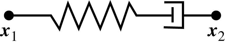
Schematic of Maxwell element.

First we consider a single viscoelastic element between the nodes
 $\boldsymbol{x}_{1}(t)$
and
 $\boldsymbol{x}_{2}(t)$
immersed in a viscous fluid; see figure 2. In this case, the element exerts a restoring force given by
 $$\begin{eqnarray}\boldsymbol{f}_{s}(\boldsymbol{x}_{1})=-\boldsymbol{f}_{s}(\boldsymbol{x}_{2})=\ell _{0}^{2}E\left(\frac{\Vert \boldsymbol{x}_{2}-\boldsymbol{x}_{1}\Vert }{\ell (t)}-1\right)\frac{\boldsymbol{x}_{2}-\boldsymbol{x}_{1}}{\Vert \boldsymbol{x}_{2}-\boldsymbol{x}_{1}\Vert },\end{eqnarray}$$
where
 $\ell (t)$
denotes the element resting length,
 $E$
the spring stiffness constant and
 $\ell _{0}=\ell (0)$
an initial resting length. Since the force required to open a dashpot is proportional to the rate of change of the length of the element, the model is just an elastic spring whose resting length
 $\ell (t)$
changes dynamically as the spring is stretched or contracted. When the spring is stretched, the resting length must increase to simulate the opening of the dashpot. The model that sets the rate of change of the spring resting length proportional to the spring force is
 $$\begin{eqnarray}\frac{\text{d}\ell (t)}{\text{d}t}=\frac{E\ell _{0}}{{\it\eta}}\left(\frac{\Vert \boldsymbol{x}_{2}-\boldsymbol{x}_{1}\Vert }{\ell (t)}-1\right),\end{eqnarray}$$
where
 ${\it\eta}$
denotes the dashpot constant. Note that if the viscosity constant
 ${\it\eta}\rightarrow \infty$
in (2.8), there would be no change in the element’s resting length, and the link would be a simple elastic spring. For viscoelastic networks, such as that depicted in figure 5(a), the force at node
 $\boldsymbol{x}_{i}(t)$
is given by
 $$\begin{eqnarray}\boldsymbol{g}(\boldsymbol{x}_{i})=\mathop{\sum }_{j}\ell _{0,ij}^{2}E_{ij}\left(\frac{\Vert \boldsymbol{x}_{j}-\boldsymbol{x}_{i}\Vert }{\ell _{ij}(t)}-1\right)\frac{\boldsymbol{x}_{j}-\boldsymbol{x}_{i}}{\Vert \boldsymbol{x}_{j}-\boldsymbol{x}_{i}\Vert },\end{eqnarray}$$
where the
 $\boldsymbol{x}_{j}$
are all neighbour nodes connected to
 $\boldsymbol{x}_{i}$
,
 $E_{ij}$
is a stiffness and
 $\ell _{ij}(t)$
is the resting length of the link between node
 $\boldsymbol{x}_{i}$
and
 $\boldsymbol{x}_{j}$
that satisfies the relation (2.8).
When the links of the elements comprising a network are disturbed from their equilibrium configuration, an elastic potential energy develops:
 $$\begin{eqnarray}PE(t)=\mathop{\sum }_{j<i}\mathop{\sum }_{i}\ell _{0,ij}^{3}E_{ij}\left(\frac{\Vert \boldsymbol{x}_{j}-\boldsymbol{x}_{i}\Vert }{\ell _{ij}(t)}-1\right)^{2}.\end{eqnarray}$$
We first consider a regular cubic network as in figure 5(a) that is constructed of
 $m\times m\times m$
equally spaced nodes. A length scale is chosen so that the non-dimensional lengths of the sides of the cube are one. We designate
 $3m^{2}(m-1)$
viscoelastic elements that connect adjacent points in the directions aligned with the unperturbed cube faces. We can also consider networks with higher connectivity that add diagonal links so that each interior node is connected to its twenty-six neighbours; see figure 6(e). This cubic high-connectivity network is composed of
 $(13m^{2}-14m+4)(m-1)$
links. Of course, these are idealized structures but present a starting point for representing more biologically realistic networks. More random structures that are perturbations of these networks will be discussed below.
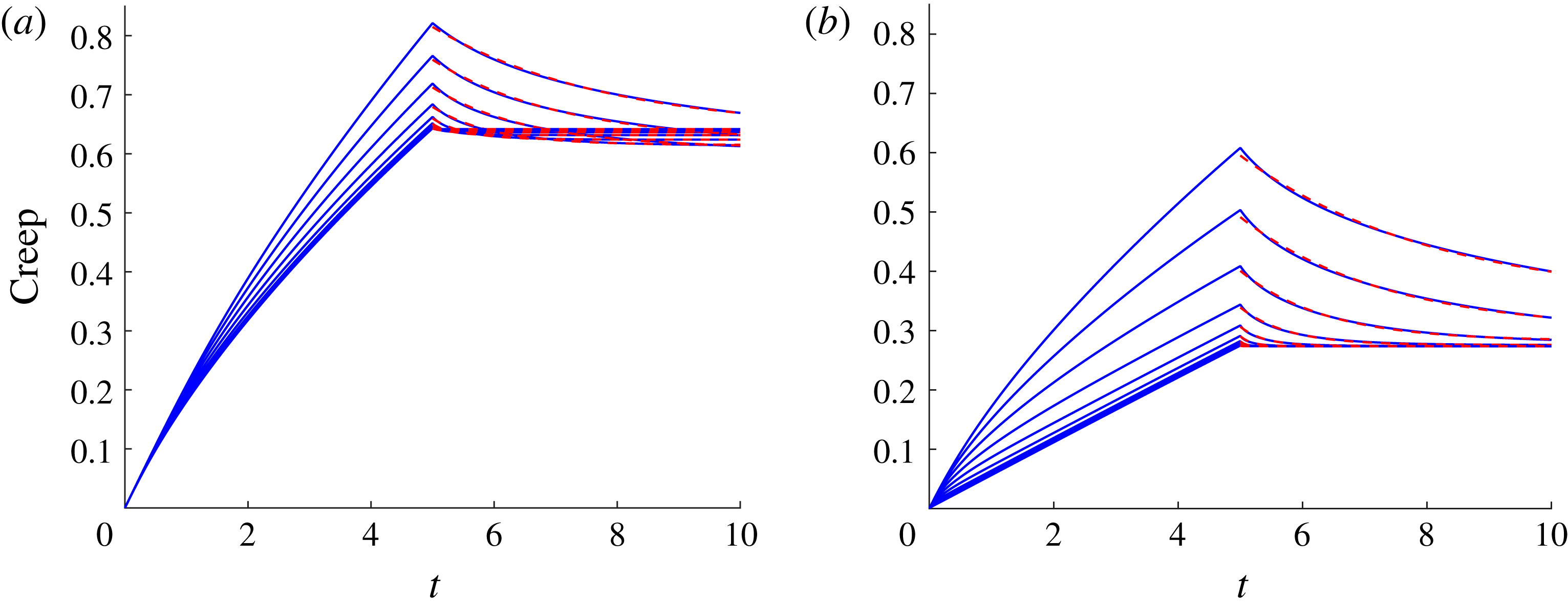
As in Wróbel et al. (Reference Wróbel, Cortez and Fauci2014), and using the non-dimensionalization presented therein, we characterize the non-dimensional relaxation time of these regular networks by subjecting them to a computational creep test. We measure the behaviour of the viscoelastic material by applying a constant stress to the top layer of the network in a coordinate direction parallel to the layer. These forces are communicated through the background viscous fluid, and the nodes of the mesh move with the resulting fluid velocity determined by (2.3). The network deforms as the top layer slides, and the individual Maxwell elements also generate force on the viscous fluid. The constant stress is then turned off, and the viscoelastic network relaxes. We compute the evolving strain at the top plate as a function of time. Figure 3(a,b) show the resulting creep functions for both the low connectivity and high connectivity
 $8\times 8\times 8$
networks, respectively, where all links in the network are assigned the same spring constant
 $E$
and dashpot parameter
 ${\it\eta}$
. Results for a range of elastic spring constants
 $E$
and the fixed dashpot parameter
 ${\it\eta}=10$
are shown. In order to assign a relaxation time to the viscoelastic structure, an exponential decaying function is fitted to the unloaded phase of the creep functions. Here, for the range of
 $0.625<E<320$
, the relaxation times for the low-connectivity network are
 $2.78>{\it\tau}>0.017$
and
 $3.12>{\it\tau}>0.012$
for the high connectivity network, with
 ${\it\tau}$
decreasing as
 $E$
increases. Note that we non-dimensionalize time by the temporal period of a flagellar beat, so this relaxation time may be thought of as effective Deborah number for the coupled swimmer–network system.
Creep functions for the viscoelastic network whose top surface is subject to a unit stress. The response of the network is shown for (a) low connectivity and (b) high connectivity networks with ten different stiffness parameters
 $E=0.625\times 2^{0{-}9}$
for a fixed damping constant
 ${\it\eta}=10$
. Exponentially decaying functions are fitted to the unloading phase of the creep (dashed line). In each case, the non-dimensional viscosity
 ${\it\mu}=1$
and the blob parameter was
 ${\it\delta}=1/4{\rm\pi}$
.

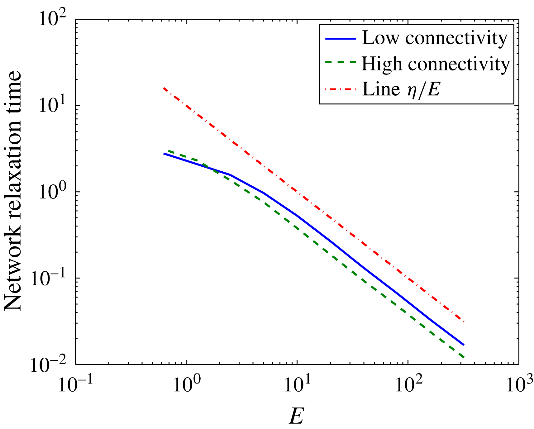
These creep functions in figure 3(a,b) show that the high-connectivity network is stiffer than the network with low connectivity. The high-connectivity network does not deform as much as the one with fewer structural links, and it relaxes more rapidly when the stress is turned off. Because of the dashpot in the Maxwell elements, the strain does not approach zero. Figure 4 shows a log–log plot of the relaxation time as a function of the non-dimensional elasticity parameter
 $E$
for the low and high connectivity networks.
Relaxation times for both low- and high-connectivity networks as a function of
 $E$
computed using a computational creep test. The relaxation time of a single Maxwell element
 ${\it\eta}/E$
is plotted for reference. All computations used
 ${\it\eta}=10$
.

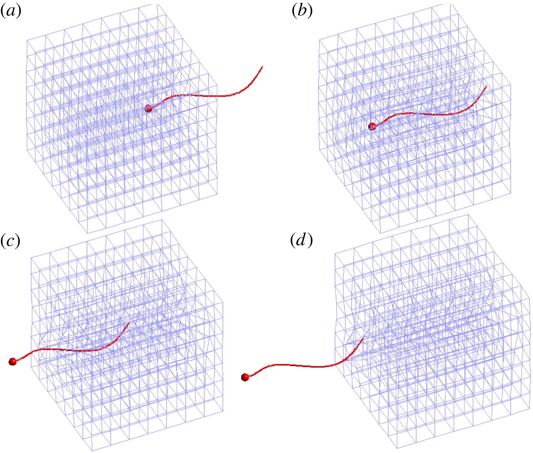
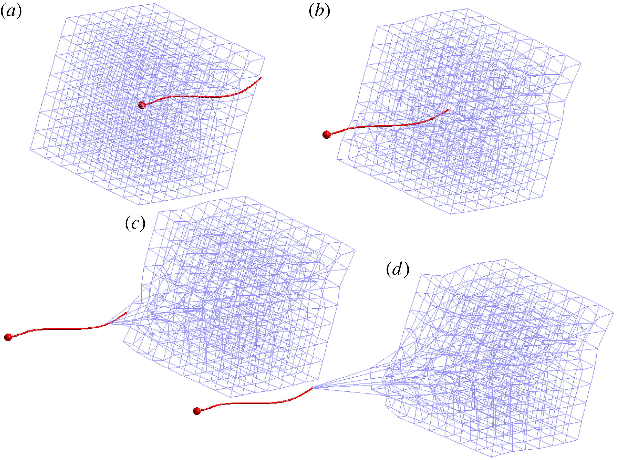
Swimmer moving through the low-connectivity cubic viscoelastic network composed of 1344 links at times
 $t=15$
, 25, 35, 45, respectively. Note that the temporal period of a flagellar beat is
 $t=1$
. Here the stiffness parameter of each Maxwell element is
 $E=10$
, the damping parameter is
 ${\it\eta}=10$
and the network relaxation time is
 ${\it\tau}=0.53$
. See supplementary movie 1 available at http://dx.doi.org/10.1017/jfm.2016.99.

Swimmer moving through the high-connectivity viscoelastic network composed of 5068 links at times
 $t=15$
, 25, 35, 45, respectively. Note that the temporal period of a flagellar beat is
 $t=1$
. Here the stiffness parameter of each Maxwell element is
 $E=10$
, the damping parameter is
 ${\it\eta}=10$
, and the relaxation time is
 ${\it\tau}=0.40$
. See supplementary movie 2.

2.3 Coupled network–swimmer model
Here we describe the algorithm that couples the dynamics of the viscoelastic network and the flagellar swimmer immersed in a 3-D Stokesian fluid. The cell body and the flagellum of the swimmer at time step
 $n$
are discretized by
 $N=N_{c}+N_{f}$
nodes
 $\boldsymbol{x}_{k}$
for
 $k=1,\ldots ,N$
. Using the prescribed waveform in (2.5), the prescribed body velocities
 $\boldsymbol{u}_{\boldsymbol{b}_{k}^{n}}$
may be calculated by differentiation with respect to
 $t$
. At time step
 $n$
the
 $N_{v}=m\times m\times m$
nodes of the viscoelastic network are
 $\boldsymbol{y}_{j}^{n}$
for
 $j=1,\ldots ,N_{v}$
. The time-stepping algorithm proceeds as follows:
Given the network nodes
 $\boldsymbol{y}_{j}^{n}$
for
 $j=1,\ldots ,N_{v}$
, and the body velocities
 $\boldsymbol{u}_{\boldsymbol{b}_{k}^{n}}$
imposed on the swimmer nodes
 $\boldsymbol{x}_{k}^{n},k=1,\ldots ,N$
:
-
(i) Compute the
 $N_{v}$
forces
$\boldsymbol{g}_{j}^{n}$
for
$j=1,\ldots ,N_{v}$
at these network nodes due to the deformation of the Maxwell elements using (2.9).
-
(ii) Evaluate (2.3) at the
$N$
swimmer nodes
$\boldsymbol{x}_{k}^{n}$
to find the velocities that would be induced by the
$N_{v}$
viscoelastic forces
$\boldsymbol{g}_{j}^{n}$
in the absence of any other forces. Call these auxiliary velocities
$\bar{\boldsymbol{U}}_{k}^{n},k=1,\ldots ,N$
. -
(iii) Use the linear system in (2.6a ) and (2.6b,c ) with the left-hand side of (2.6a ) replaced by
$\boldsymbol{u}_{\boldsymbol{b}_{j}^{n}}-\bar{\boldsymbol{U}}_{j}^{n}$
to solve for the translational velocity
$\boldsymbol{U}^{n}$
, rotational velocity
${\it\bf\Omega}^{n}$
and the forces
$\boldsymbol{f}_{k}^{n},k=1,\ldots ,N$
on the swimmer. -
(iv) Given the distribution of forces
$\boldsymbol{f}_{k}^{n},k=1,\ldots ,N$
and
$\boldsymbol{g}_{k}^{n},k=1,\ldots ,N_{v}$
at the swimmer nodes and the network nodes, respectively, use (2.3) to evaluate the velocities
$\boldsymbol{V}_{j}^{n+1}$
at the network nodes
$\boldsymbol{y}_{j}^{n},j=1,\ldots ,N_{v}$
due to all
$N+N_{v}$
forces. -
(v) Update the position of the network nodes:
(2.11)
$$\begin{eqnarray}\boldsymbol{y}_{j}^{n+1}=\boldsymbol{y}_{j}^{n}+{\rm\Delta}t\boldsymbol{V}_{j}^{n+1},\quad j=1,\ldots ,N_{v}.\end{eqnarray}$$
-
(vi) Update the position of the swimmer nodes:
(2.12)where
$$\begin{eqnarray}\boldsymbol{x}_{k}^{n+1}=\boldsymbol{x}_{k}^{n}+{\rm\Delta}t(\boldsymbol{U}^{n}+{\it\bf\Omega}^{n}\times (\boldsymbol{x}_{k}^{n}-\boldsymbol{x}_{c}^{n})+\boldsymbol{u}_{\boldsymbol{ b}_{k}^{n}}),\quad k=1,\ldots ,N_{v},\end{eqnarray}$$
$\boldsymbol{x}_{c}^{n}$
is the centroid of the cell body at time step
$n$
.


Here
 ${\rm\Delta}t$
is a time step. This algorithm does allow the viscoelastic network geometry to respond to the evolving fluid flow. However, we remark that this algorithm does not represent a fully coupled system, since the kinematics of the flagellar swimmer are pre-set and do not respond to the evolution of the viscoelastic mesh.
3 Results
We present examples in which a microorganism swims in a viscous Newtonian fluid and encounters a heterogeneous viscoelastic structure suspended in the viscous environment. The heterogeneous medium is represented by the viscoelastic network submerged in a Stokes flow. The organism swims and enters the embedded elastic network, interacts with it as it deforms and eventually exits the network. In all examples we use a network of
 $8\times 8\times 8$
nodes connected by Maxwell virtual elements. We refer to them as virtual because a Maxwell link connecting two nodes is only used to compute the forces at those nodes but does not represent a solid obstacle to the swimming microorganism. Initially, the network is a unit cube, and this unit length is also the total arclength of the swimmer’s flagellum.
The connectivity of the network nodes matters. As shown above, two networks with the same set of nodes can display different responses to a perturbation if the nodes in one network are connected to more neighbours than the other. Here we report results from the two different connectivities discussed in § 2.2 above. In the low connectivity network, each internal node is connected to six neighbours (the six nearest nodes in a cubic lattice) and in the high-connectivity network, each internal node is connected to 26 neighbours (the 26 nearest nodes in a cubic lattice).
3.1 A cubic network aligned with the axes
In this example, the network is a cubic lattice of unit side length so that the initial length of every virtual link is
 $\ell _{k}(0)=0.1428$
. The network is centred at the origin and the microorganism starts swimming along the
 $x$
-axis toward the network with the centre of the spherical cell at
 $(1,0,0)$
. The dimensionless flagellar length is one, the diameter of the cell is 0.0555 and the parameter values used are
 $E=10$
and
 ${\it\eta}=10$
. The computed relaxation time of this low connectivity network is
 ${\it\tau}=0.53$
. Figure 5 shows snapshots of the motion of the microorganism and the deformation of the low-connectivity network as the organism makes its way through it. Figure 6 shows snapshots of the motion of the microorganism and the deformation of the high-connectivity network at the same instances in time.
The forward swimming speed – the projection of the swimmer’s velocity onto its forward direction – is averaged over a flagellum oscillation period (
 $T=1$
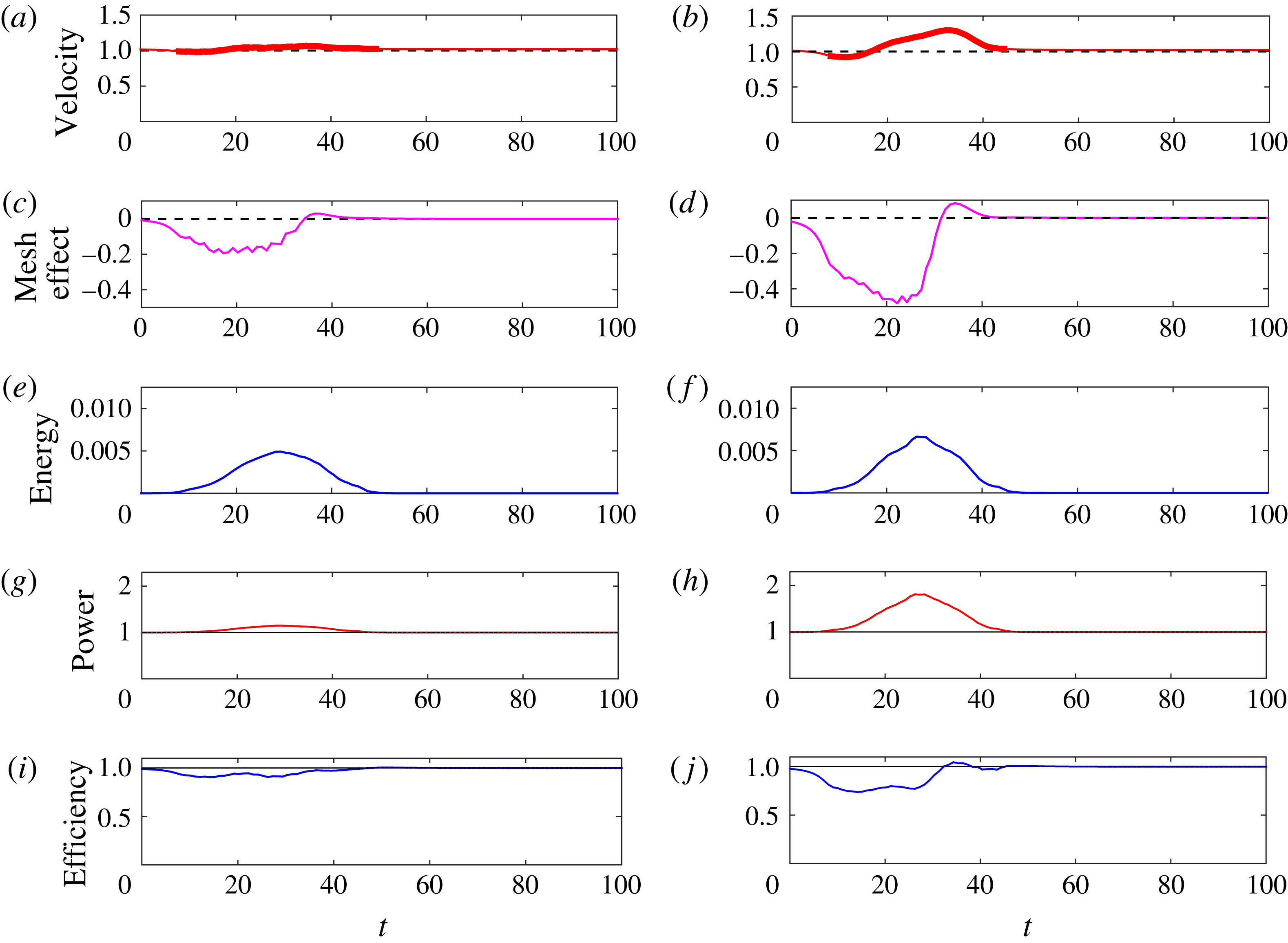
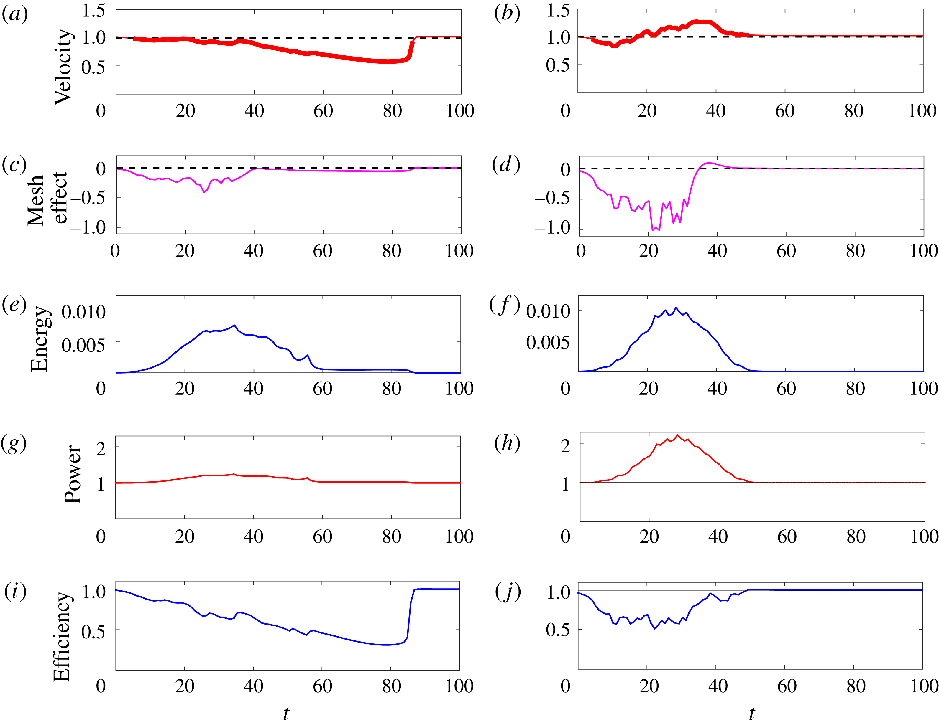
) and normalized by its swimming speed in the absence of the network. The result is plotted in figure 7(a) for the low-connectivity network and figure 7(b) for the high-connectivity one. The bold part of the curve indicates the times when any part of the organism was inside the network structure.
Swimmer through cubic network with Maxwell elements of stiffness
 $E=10$
and damping
 ${\it\eta}=10$
. Swimming velocity normalized by the velocity of the same swimmer in Stokes flow (a) low connectivity (b) and high connectivity. The bold part of the curve indicates that a swimmer node is inside the network. Mesh-effect velocity normalized by network-free swimming velocity (c) low connectivity (d) high connectivity. Potential energy of the network (e) low connectivity (f) high connectivity. Power expended by swimmer normalized by the power expended by the same swimmer in Stokes flow (g) low connectivity (h) high connectivity. Efficiency of swimmer normalized by the efficiency of same swimmer in Stokes flow (i) low connectivity (j) high connectivity.

A comparison of figures 7(a) and 7(b) shows the effect of the different connectivity for the same set of network nodes. For the structure with lower connectivity, the swimming speed oscillates only slightly around the network-free speed. The high-connectivity network shows a more pronounced deviation, where the forward swimming slows down as the microorganism approaches and enters the network. Once the organism is inside and as it exits the network, its swimming speed gets a boost when compared to the network-free case. When the organism is completely out of the network, its speed goes back to the network-free speed.
Does the stored elastic energy in the viscoelastic network help or hinder the swimmer? As the network elements contract or expand, they develop forces at the nodes which affect the motion of the organism. Because of the linearity of the system, we can isolate the instantaneous cell speed due only to the network by computing the network force velocity contribution to the cell motion while ignoring the forces at the nodes of the swimmer. This network contribution to the cell velocity is computed by evaluating the velocity due to the network forces at the cell body centroid, and then projecting this onto the direction of swimming. Figure 7(c,d) show this mesh-effect speed normalized by the network-free swimming speed. The figures indicate that the instantaneous cell speed due only to the network initially is negative (opposes forward motion), but once the organism begins to exit the structure, the instantaneous cell speed due to the network is positive (in the direction of forward motion). The time of largest swimming speed corresponds to the maximum contribution by the network. We note that even when the network has a negative contribution to the cell speed, the organism may progress faster or slower than in a Newtonian fluid because the beating of the flagellum has been prescribed and the organism forces are computed to meet the prescribed beat regardless of any network effects. Moreover, the computation of forces on the flagellum uses information from the elastic deformation of the network.
The evolution of the potential energy (2.10) stored in the network elements is shown in figure 7(e,f). Although the network does not relax to its initial configuration due to the changing resting lengths of the Maxwell elements, the figures show that the potential energy reaches a maximum and decays to zero at about the time when then swimming speed settles to the network-free speed.
In this idealized system the gait of the flagellar swimmer is prescribed without any feedback from the evolving network. We measure the power that must be expended by the flagellum to maintain this gait as it progresses into and through the viscoelastic structure:
 $$\begin{eqnarray}P(t)=\mathop{\sum }_{k=1}^{N_{f}}\boldsymbol{u}(\boldsymbol{x}_{k}(t))\boldsymbol{\cdot }\boldsymbol{f}_{k}(t){\rm\Delta}s,\end{eqnarray}$$
where
 $\boldsymbol{x}_{k}$
are the flagellar nodes,
 $\boldsymbol{f}_{k}$
are the forces at these nodes and
 ${\rm\Delta}s$
is the spacing between nodes. Figure 7(g,h) show this power normalized by the power for a network-free swimmer, for both the low- and high-connectivity networks. We see that evolution of power follows the same pattern as the potential energy – reaching a maximum when the swimmer is inside the network, but then begins to decrease at the same time as the instantaneous cell speed due to the network starts to increase. When the swimmer leaves the network the power requirements return to that of the network-free case. We also measure the efficiency
 $EF(t)=V^{2}/P$
of swimming, where
 $V$
is the forward swimming speed. Figure 7(i,j) show this efficiency normalized by that of a network-free swimmer for both the low- and high-connectivity networks. For most of the swimmer’s path, the presence of the viscoelastic network results in lower efficiency. However, in the high-connectivity network, we see a slight increase in efficiency as the swimmer exits the network.
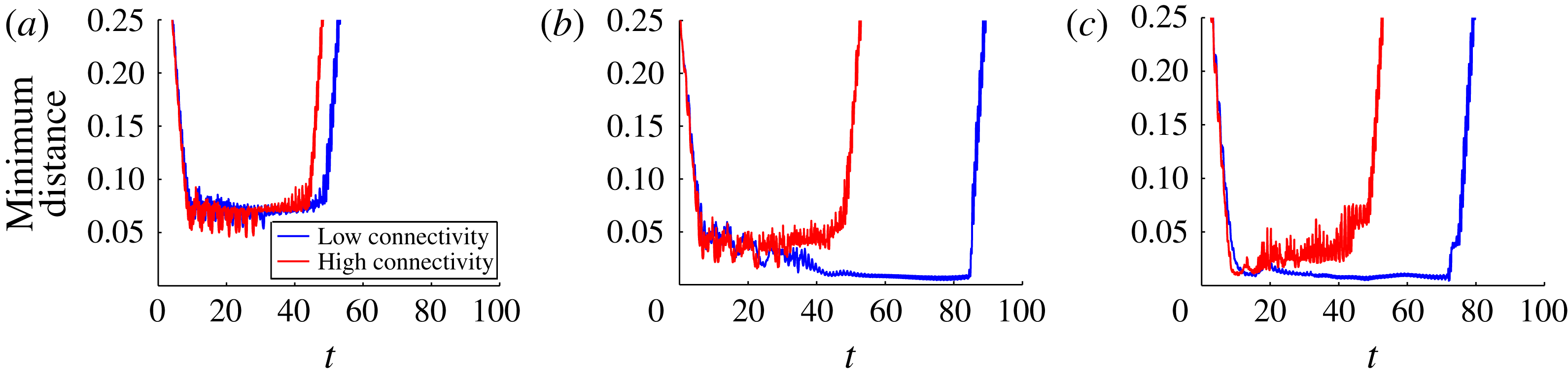
The discrete nature of the network nodes influences the swimming progression depending on the position of the microorganism relative to the nodes. The minimum distance between any point on the organism and any network node throughout the simulations in figures 5 and 6 is shown in figure 8(a). For both types of connectivity, this distance is never smaller than about one cell body diameter. However, this result may change if the organism approaches a face of the network at an angle or if the network is not uniform. We consider these cases next.
The minimum distance between the organism and the network nodes for both the low- and high-connectivity cubic networks (a) regular cubic network, (b) rotated cubic network, (c) randomly perturbed network.

3.2 A tilted cubic network
When the microorganism approaches a face of the cubic network at an angle between 0 and
 $90^{\circ }$
, there is a different likelihood that the organism will come close to a network node and experience a higher resistance to its swimming motion. In this example the organism swims initially along the
 $x$
-axis toward the network as before, but the network has been rotated slightly (see figure 9 in the case of low connectivity). The computation of the forward swimming speed, the effect of the network on this speed, the potential energy stored in the network and power expenditure are shown in figure 10 for both connectivities, and should be compared to figure 7.
Swimmer moving through the low-connectivity rotated cubic viscoelastic network composed of 1344 links at times
 $t=20$
, 40, 60, 80, respectively. Note that the temporal period of a flagellar beat is
 $t=1$
. Here the stiffness parameter of each Maxwell element is
 $E=10$
and the damping parameter is
 ${\it\eta}=10$
. See supplementary movies 3 and 4.

For the high-connectivity network, figure 10(b,d,f,h) shows that the tilt angle did not affect the results significantly, although a boost in efficiency as the swimmer leaves the network is not prominent in figure 10(j). Some of the fluctuations are more pronounced and the instantaneous cell speed due to the network is larger in magnitude than when the tilt angle was 0. Figure 8(b) shows that the organism came closer than before to network nodes to within half of a cell diameter. On the other hand, the low-connectivity case is significantly different. Figure 9 shows that the organism came so close to at least one network node (figure 8 b) that it dragged it a substantial distance. As a consequence, it took the organism much longer to swim through the network as the swimming speed was significantly lower (figure 10 a). By the time the organism was exiting the network, most of the Maxwell elements had had enough time to relax to their new equilibrium lengths and there was not enough potential energy stored in the network to have a significant effect on the organism’s swimming speed, which simply rose to the network-free value.
Swimmer through rotated cubic network with Maxwell elements of stiffness
 $E=10$
and damping
 ${\it\eta}=10$
. Swimming velocity normalized by the velocity of the same swimmer in Stokes flow (a) low connectivity (b) and high connectivity. The bold part of the curve indicates that a swimmer node is inside the network. Mesh-effect velocity normalized by network-free swimming velocity (c) low connectivity (d) high connectivity. Potential energy of the network (e) low connectivity (f) high connectivity. Power expended by swimmer normalized by the power expended by the same swimmer in Stokes flow (g) low connectivity (h) high connectivity. Efficiency of swimmer normalized by the efficiency of same swimmer in Stokes flow (i) low connectivity (j) high connectivity.

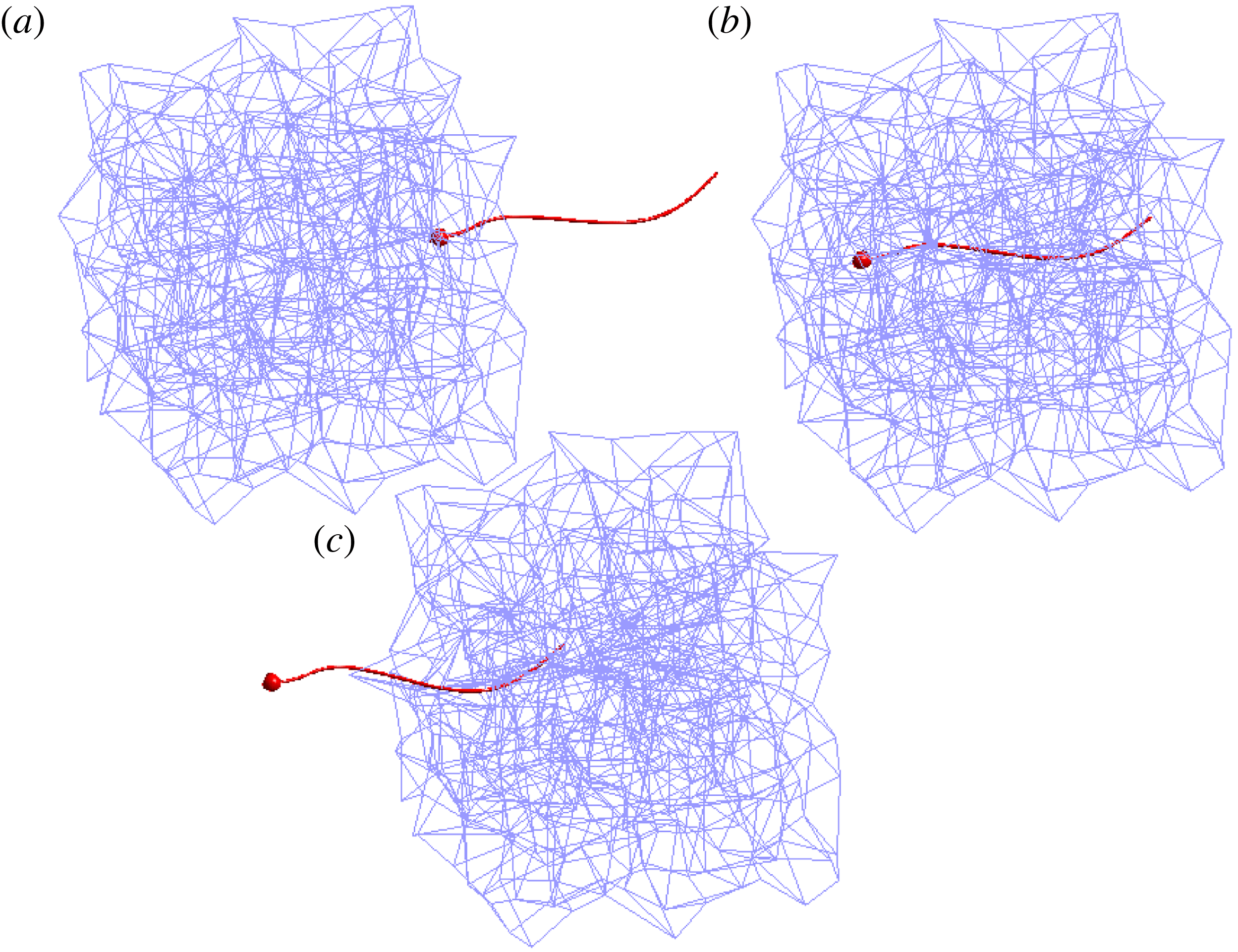
Swimmer moving through the low-connectivity perturbed viscoelastic network composed of 1344 links at times
 $t=10$
, 30, 50. Note that the temporal period of a flagellar beat is
 $t=1$
. Here the stiffness parameter of each Maxwell element is
 $E=10$
and the damping parameter is
 ${\it\eta}=10$
. See supplementary movie 5.

Swimmer moving through the high-connectivity perturbed viscoelastic network composed of 5068 links at times
 $t=10$
, 30, 50. Note that the temporal period of a flagellar beat is
 $t=1$
. Here the stiffness parameter of each Maxwell element is
 $E=10$
and the damping parameter is
 ${\it\eta}=10$
. See supplementary movie 6.

3.3 A randomly perturbed network
A network without symmetries can be created by starting with the cubic network and then randomly perturbing the node locations by a fraction of the original spacing. In this case we still have the same number of nodes as before and the connectivity of each node is retained from the unperturbed cases. A randomly perturbed network is shown in figures 11 and 12 with the two types of connectivities. One noticeable difference that is evident in this figure compared to previous examples is that the microorganism experiences more rotation in the high-connectivity case. Although the flagellum in figure 12(c) looks straight, it is in fact sinusoidal but it has rotated so that it appears straight from the perspective of the figure.
Swimmer through perturbed viscoelastic networks with Maxwell elements of stiffness
 $E=10$
and damping
 ${\it\eta}=10$
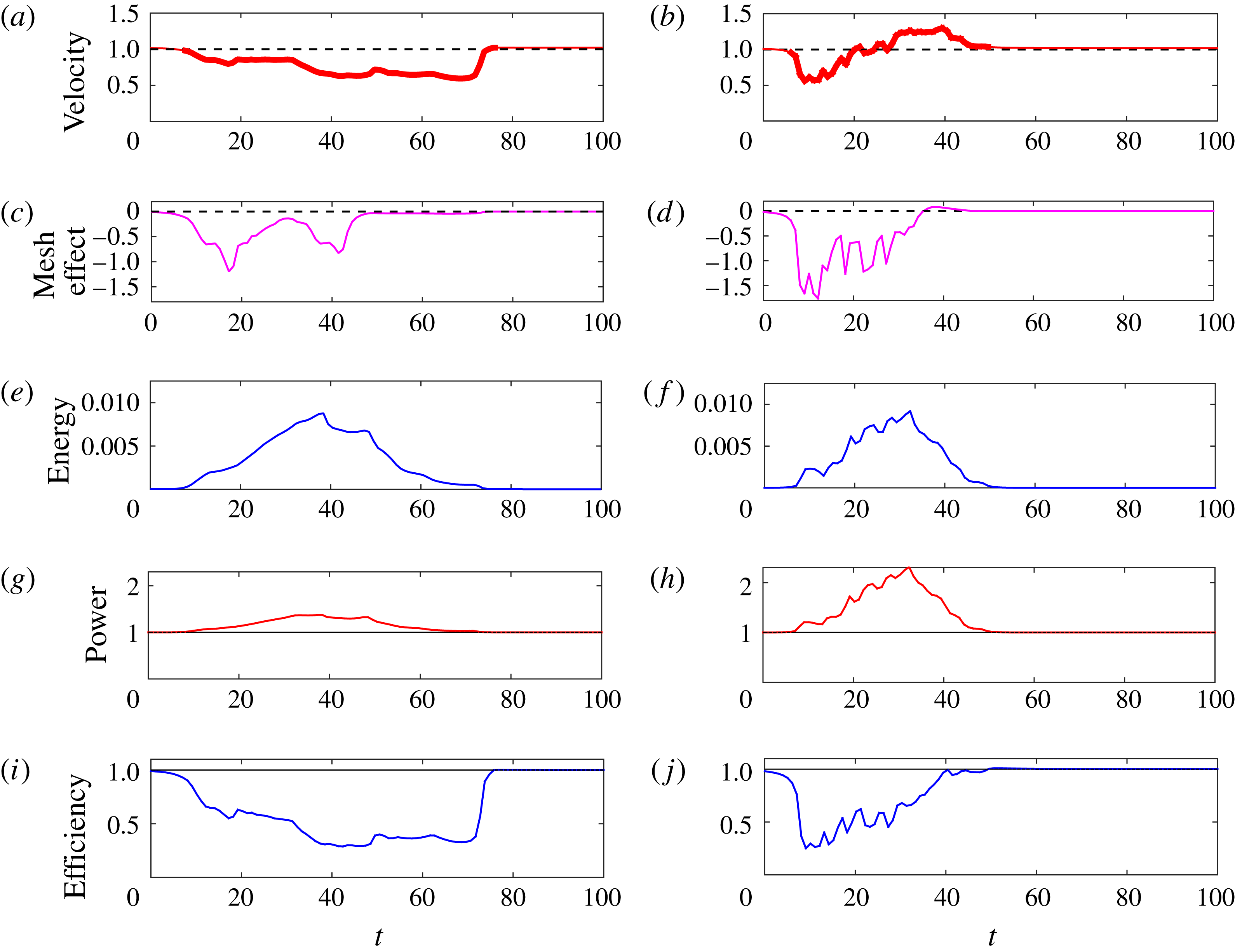
. Swimming velocity normalized by the velocity of the same swimmer in Stokes flow (a) low connectivity (b) and high connectivity. The bold part of the curve indicates that a swimmer node is inside the network. Mesh-effect velocity normalized by network-free swimming velocity (c) low connectivity (d) high connectivity. Potential energy of the network (e) low connectivity (f) high connectivity. Power expended by swimmer normalized by the power expended by the same swimmer in Stokes flow (g) low connectivity (h) high connectivity. Efficiency of swimmer normalized by the efficiency of same swimmer in Stokes flow (i) low connectivity (j) high connectivity.

Figure 13 shows the forward swimming speed, the instantaneous cell speed due to the network, the potential energy stored in the network and the power and efficiency, all of which look qualitatively similar to those in figure 10. The curves corresponding to the randomly perturbed network show larger fluctuations and indicate that the microorganism is likely to come close to some of the nodes (figure 8 c). In fact, the velocity of the swimmer in the low-connectivity network (figure 13 a) is slow enough that stored energy due to the Maxwell elements relaxes nearly to zero even when part of the organism is still in the network (figure 13 e).
3.4 Effects of stiffness variation
The examples presented so far have used fixed values of the Maxwell element parameters. We perform similar simulations with the cubic networks of figures 5 and 6 with
 ${\it\eta}=10$
but varying values of
 $E$
(we use the same parameter values for all elements in a given simulation). Although
 ${\it\eta}/E$
is a relaxation time for a single Maxwell element, the network as a whole develops its own effective relaxation time, and we compute this as described in § 2.2 using a computational creep test (see figure 4). The resulting non-dimensional relaxation times of the network fall in the range
 $2.78>{\it\tau}>0.017$
(low connectivity) and
 $3.12>{\it\tau}>0.012$
(high connectivity).
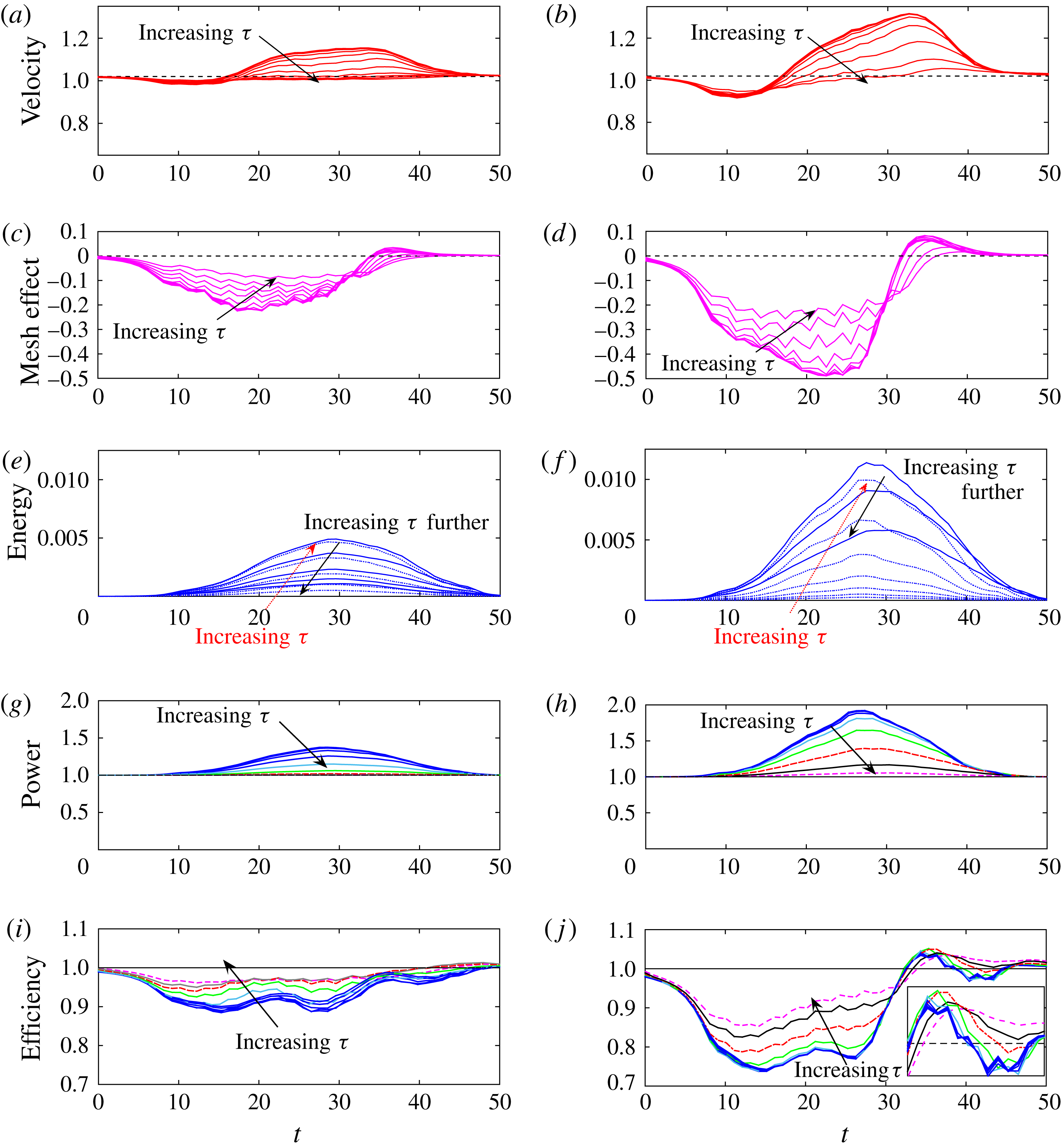
We track the swimmer’s velocity, the instantaneous cell speed due to the network, potential energy in the network, power expended by the swimmer and efficiency, and indicate how these curves change with the relaxation time of the network
 ${\it\tau}$
in figure 14. Figure 14(a,b) show that the shape of the swimming speed curves are similar to those of the cubic network cases presented earlier, but deviate more from the network-free swimming speed for smaller values of the network relaxation time
 ${\it\tau}$
(larger spring stiffness
 $E$
). The swimming speed decreases as the organism enters the network and experiences a boost as it exits. This boost is larger for small values of
 ${\it\tau}$
. When
 ${\it\tau}$
is large, the network is floppy and has less of an effect on the swimmer, resulting in a more uniform swimming speed throughout the simulation (as in a Newtonian fluid). This conclusion is supported by figure 14(c,d) that show that the instantaneous cell speed due to the network is largest in magnitude for small
 ${\it\tau}$
and is reduced as
 ${\it\tau}$
increases. Note that as
 ${\it\tau}$
decreases, the curves saturate, indicating that for large values of
 $E$
the network elements are stiff and the network acts as a rigid cage within the fluid. The nodes develop forces that keep the structure rigid and affect the organism’s swimming speed.
Results of the coupled swimmer–network system in both the low- and high-connectivity networks with ten different stiffness parameters
 $E=0.625\times 2^{0{-}9}$
for a fixed damping constant
 ${\it\eta}=10$
. Relaxation time of network computed by creep test is
 ${\it\tau}$
, and falls in the range
 $2.78>{\it\tau}>0.017$
(low connectivity) and
 $3.12>{\it\tau}>0.012$
(high connectivity). Swimming velocity normalized by the velocity of the same swimmer in Stokes flow (a) low connectivity (b) high connectivity. Mesh-effect velocity normalized by network-free swimming velocity (c) low connectivity (d) high connectivity. Potential energy of the network (e) low connectivity (f) high connectivity. Power expended by swimmer normalized by the power expended by the same swimmer in Stokes flow (g) low connectivity (h) high connectivity. Efficiency of swimmer normalized by the efficiency of same swimmer in Stokes flow (i) low connectivity (j) high connectivity.

Figure 14(e,f) show the evolution of the potential energy in the low- and high-connectivity viscoelastic networks, respectively. For each set of parameters the potential energy reaches a maximum value as the swimmer moves through the network, and then relaxes to zero as the swimmer moves out. However, as indicated in figure 14(e,f), the maximum potential energy is not monotonic in the relaxation time
 ${\it\tau}$
. For very stiff networks (small
 ${\it\tau}$
) the flagellar beating causes little network distortion, and the potential energy developed is small. As
 ${\it\tau}$
increases, the network becomes more compliant, experiences greater deformation and, hence, stores more potential energy. However, increasing
 ${\it\tau}$
even more (decreasing the elastic parameter
 $E$
) represents very floppy links and, hence, the maximal potential energy stored decreases.
Figure 14(g,h) show the evolution of the power expenditure by the swimmers as they move through the low- and high-connectivity networks. Here the behaviour is again monotonic in the relaxation time
 ${\it\tau}$
. Stiffer networks require more power from the organism to achieve its prescribed gait. Figure 14(i,j) show the evolution of the swimming efficiency normalized by the efficiency of the same swimmer in Stokes flow. Again, we see that all swimmers achieve lower efficiencies as they move through the network, while those in the high-connectivity network achieve a boost as they exit. This boost is non-monotonic in
 ${\it\tau}$
(see inset of figure 14
f).
3.5 A larger network
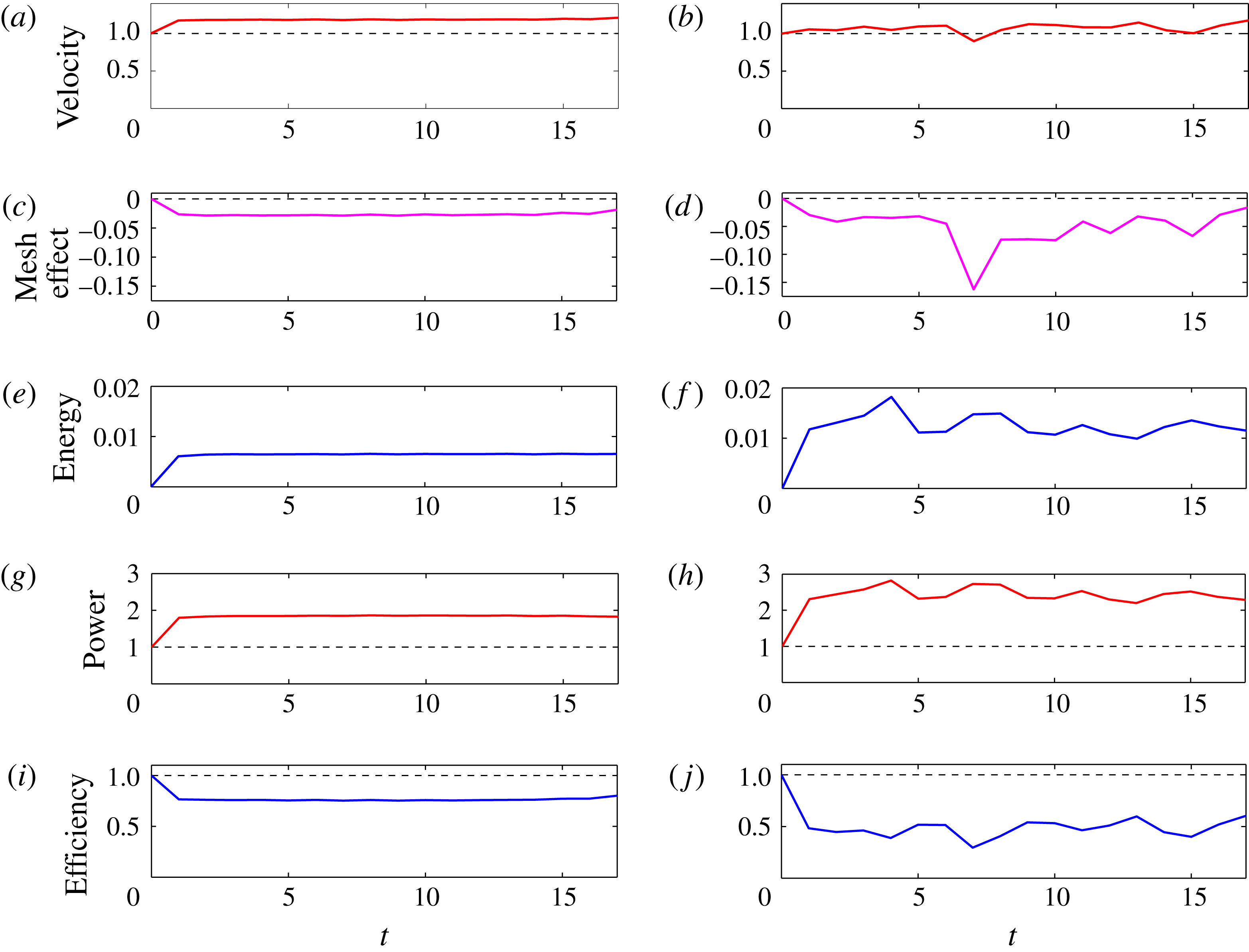
Here we present results of simulations where the swimmer moves through viscoelastic networks that are twice as long in the direction of swimming compared to previous simulations. In order to eliminate entrance and exit effects, the swimmer is launched totally within the mesh, and follow its progression during the time that it remains within the mesh. Figure 15 shows the results of two simulations of the swimmer moving within a high-connectivity regular network (a,c,e,g,i) and a high-connectivity perturbed network (b,d,f,h,j). We see that the swimmer in the regular network reaches a steady state, with an increased velocity (figure 15 a) and negative mesh effect (figure 15 c). The potential energy in the system also stabilizes as the flagellum periodically disturbs the Maxwell links it encounters as it moves through the uniform mesh (figure 15 e). The power expended by the swimmer in the regular network is almost double that required to maintain its gait in Stokes flow (figure 15 g), and we see that the efficiency is always below the Newtonian case (figure 15 i). For the corresponding swimmer in the high-connectivity perturbed mesh, Figure 15(b,d,f–h) show that these quantities fluctuate due to the discrete nature of the network and the relative position of the nodes and the swimmer as it progresses. In particular, the power expended by the swimmer in this perturbed network is even greater than that in the regular network (figure 15 h), and the same is true of the potential energy (figure 15 f).
Swimmer through double, high-connectivity viscoelastic networks composed of Maxwell elements of stiffness
 $E=10$
and damping
 ${\it\eta}=10$
. Swimming velocity normalized by the velocity of the same swimmer in Stokes flow (a) regular network (b) perturbed network. The swimmer is in the network throughout the simulation. Mesh-effect velocity normalized by network-free swimming velocity (c) regular network (d) perturbed network. Potential energy of the network (e) regular network, (f) perturbed network. Power expended by swimmer normalized by the power expended by the same swimmer in Stokes flow (g) regular network, (h) perturbed network. Efficiency of swimmer normalized by the efficiency of same swimmer in Stokes flow (i) regular network, (j) perturbed network.

By comparing these simulations of swimmers that remain within the network to the corresponding swimmers that enter, move through, and exit the same networks that were half as long (regular network: figure 7(b,d–h) and perturbed network: figure 13(b,d–h)), we can isolate some boundary effects. One such effect occurs as the swimmer in the Newtonian fluid approaches the compliant network. Its velocity is smaller than that in the network-free case, which suggests that the network develops forces that resist the forward swimming. However, for a swimmer totally within the network, figure 15 shows that the swimming speed remains roughly constant but with variations introduced by the discrete nature of the system and the near encounters of the swimmer with network nodes. Another boundary effect occurs when the swimmer exits the viscoelastic mesh. When the network stiffness is sufficiently large, the swimmer experiences a boost in speed and efficiency as it exits the network (figure 14). This only occurs if the time to cross the network is fast enough so that the dashpot elements have not yet relaxed to their equilibrium length. Figure 13(a) shows the velocity of a swimmer in a low-connectivity perturbed network. Because of interactions with the nodes, this reduced velocity resulted in a time to traverse the network that was too large compared to the Maxwell element relaxation time, so that not enough energy remained stored in the network links to help produce a boost to the swimmer as it exited.
4 Conclusion
Here we have presented a model of flagellar swimming through a viscoelastic network coupled to a Stokesian fluid in three dimensions. We measure the transient dynamics of motility as the swimmer moves from a Newtonian fluid region, into the heterogeneous medium and then out again. The discrete nodes of the compliant viscoelastic network are connected by virtual Maxwell elements that stretch or compress due to forces exerted by the swimmer and forces due to the deformations of other elements in the interconnected network. We find that swimmers with prescribed gaits can experience an enhanced swimming velocity as they enter and move through the heterogeneous network. However, more power is needed to achieve the prescribed gait in the viscoelastic network when compared to that required in a Newtonian fluid.
The increase in swimming velocity and the larger power requirements for the flagellar swimmer in the network are reminiscent of classical results in microorganism motility near boundaries. For instance, Katz (Reference Katz1974) extended Taylor’s study of swimming of an infinite sheet in an unbounded viscous fluid (Taylor Reference Taylor1951) to an infinite sheet swimming in a channel. Lubrication theory was used to show that waving near the boundaries of the channel gave the swimmer a boost, but more power was required to maintain its waveform (Katz Reference Katz1974). Our results are also consistent with the recent computational models of a finite flagellar sheet swimming through a single-phase viscoelastic fluid described by the continuum Stokes–Oldroyd-B equations (Teran et al.
Reference Teran, Fauci and Shelley2010; Thomases & Guy Reference Thomases and Guy2014). Such a system is characterized by the Deborah number (De), the ratio of the relaxation time of the fluid polymers to the characteristic flow time scale. These computations demonstrated that for swimmers with large tail amplitude whose beat period is tuned to the polymer relaxation time (
 $De\approx 1$
), the swimmer enjoys a significant speed up when compared to its velocity in a Newtonian fluid (
 $De=0$
). It is natural to ask how some properties of our discrete network model of viscoelastic elements immersed in a Stokesian fluid correspond to a continuum model of viscoelasticity, such as Oldroyd-B. Within the context of the discrete model, we can define the Deborah number to be the ratio of the mesh relaxation time
 ${\it\tau}$
to the flagellar beat period (
 $T=1$
). For the floppiest networks, the spring stiffness
 $E$
is small, the relaxation time is large and hence the Deborah number is large. However, in the extreme case of spring stiffness
 $E=0$
, no network forces are exerted on the fluid and we return to Newtonian Stokes flow. At the other extreme case, for very large spring stiffnesses, the relaxation time is small, and we approach the
 $De=0$
limit. For such stiff networks, the fluid medium is not Newtonian, but more like a Brinkman fluid with embedded obstacles. The velocity speed up demonstrated in these stiff, less compliant networks agrees qualitatively with Leshansky’s analysis that shows an enhanced swimming velocity for an infinite sheet swimming in a Brinkman fluid (Leshansky Reference Leshansky2009). This analysis indicates that the velocity of the sheet in the structured medium increases with the ratio of the sheet wavelength to obstacle spacing. For this ratio near two, the swimming of the sheet in such a medium is double that in a Stokesian fluid. However, in simulations of a finite filament swimming in a three-dimensional Brinkman fluid (closer to the system presented here), Cortez et al. (Reference Cortez, Cummins, Leiderman and Varela2010) calculate a speed up of approximately five percent. This moderate speed up is consistent with the simulations of our finite swimmer moving through the viscoelastic network.
What is not captured in a continuum model of a viscoelastic fluid are the swimmer’s velocity fluctuations as it moves through the network, and that this velocity is dependent upon the details of the network configuration. Such fluctuations were also demonstrated in the model of a reduced swimmer moving in a fluid with embedded obstacles in Jabbarzadeh et al. (Reference Jabbarzadeh, Hyon and Fu2014). In addition, we do compute the angular velocity of the flagellated swimmer, and find that the interaction of the flagellar swimmer with the network may cause it to rotate and change its swimming path.
For simplicity, we have considered simple networks whose virtual links have the same material parameters that do not change in time. Because of the discrete network formulation, one can readily incorporate dynamic element properties, such as the breaking of links in response to local network strains or stresses induced by the swimming organism. Moreover, here we have only considered swimmers whose kinematics are specified without any feedback from the local fluid environment. Within this regularized Stokeslet framework it is straightforward to replace the model swimmer described here with a flexible swimmer driven by a preferred curvature as in Olson et al. (Reference Olson, Suarez and Fauci2011), so that the gait is an emergent property of the coupled system.
Acknowledgements
This work was funded, in part, by National Science Foundation grant DMS-1043626. The work of S.L. and A.B. was conducted as Research Experiences for Undergraduates, ‘EMSW21: RTG: Mathematical and Computational Biofluids’. The authors thank H. Fu for helpful discussions.
Supplementary movies
Supplementary movies are available at http://dx.doi.org/10.1017/jfm.2016.99.