1 Introduction
The present study experimentally investigates the effects of using spanwise-modulated alternating current dielectric barrier discharge (AC-DBD) plasma actuators to condition cross-flow instability (CFI) modes. The followed strategy follows the upstream flow deformation (UFD) approach, where sub-critical stationary modes of shorter wavelength with respect to the dominant critical mode have been shown to weaken the critical mode and delay transition (Saric, Carrillo & Reibert Reference Saric, Carrillo and Reibert1998; Malik et al. Reference Malik, Li, Choudhari and Chang1999; Wassermann & Kloker Reference Wassermann and Kloker2002; Hosseini et al. Reference Hosseini, Tempelmann, Hanifi and Henningson2013). The aim of this study is to identify the pertinent interaction mechanisms between the plasma forcing and cross-flow instability modes, in view of future efforts towards transition delay.
The following sections provide an overview of the published literature on control of CFI and the background of the present study. Thorough reviews on the topic of CFI can be found in Arnal, Gasparian & Salinas (Reference Arnal, Gasparian and Salinas1998), Bippes (Reference Bippes1999) and Saric, Reed & White (Reference Saric, Reed and White2003). Some more recent studies (e.g. White & Saric Reference White and Saric2005; Bonfigli & Kloker Reference Bonfigli and Kloker2007; Serpieri & Kotsonis Reference Serpieri and Kotsonis2016) further focus on the secondary cross-flow instability.
1.1 Control of cross-flow instability
The term laminar flow control (LFC) generally describes the deployment of passive and active techniques to maintain laminar flow over aerodynamic bodies by delaying laminar-to-turbulent transition. A review of the techniques developed for this purpose was compiled by Joslin (Reference Joslin1998). Regarding the specific case of swept wings flows, the main driver of the transition process is the cross-flow instability (Saric et al. Reference Saric, Reed and White2003). The main contributions towards control of cross-flow instability are summarised in Messing & Kloker (Reference Messing and Kloker2010). In the following discussion, these are briefly described together with the more recent published efforts.
Saric et al. (Reference Saric, Carrillo and Reibert1998) introduced the idea of inducing sub-critical stationary modes, featuring smaller wavelength compared to the naturally dominant modes, to delay transition in three-dimensional (3-D) boundary layers, based on the observations of Reibert et al. (Reference Reibert, Saric, Carrillo and Chapman1996). Further investigations by Malik et al. (Reference Malik, Li, Choudhari and Chang1999), Wassermann & Kloker (Reference Wassermann and Kloker2002), Hosseini et al. (Reference Hosseini, Tempelmann, Hanifi and Henningson2013) in theoretical and numerical studies confirmed the reported positive effects, towards delaying transition. This approach, named sub-critical discrete roughness elements (DRE) (Saric et al. Reference Saric, Carrillo and Reibert1998), leads to enhanced amplification of shorter-wavelength modes by means of roughness elements forcing. The term upstream flow deformation is more generally used when making use of any device capable of inducing monochromatic modes (Wassermann & Kloker Reference Wassermann and Kloker2002). The inception of the sub-critical modes leads to a mean-flow deformation which delays the destabilisation of the critical mode thus postponing the amplification of secondary modes and, therefore, the eventual flow breakdown (Wassermann & Kloker Reference Wassermann and Kloker2002). Following the DRE/UFD concept, several studies have been carried out encompassing wind tunnel and free flight experiments as well as numerical simulations. White & Saric (Reference White and Saric2000) performed wind tunnel campaigns with pneumatically actuated surface roughness elements. Unfortunately, the device did not perform as wished because of technological issues but enhanced the interest towards active LFC based on the DRE/UFD approach. The flow case of the experiment by Saric et al. (Reference Saric, Carrillo and Reibert1998) was later investigated by Hosseini et al. (Reference Hosseini, Tempelmann, Hanifi and Henningson2013) with direct numerical simulations (DNS). Similar outcomes in terms of transition delay were obtained. The extension of the sub-critical DRE/UFD strategy to supersonic flows was demonstrated with the works of Saric & Reed (Reference Saric and Reed2002) and Schuele, Corke & Matlis (Reference Schuele, Corke and Matlis2013) for swept wings and circular cones at incidence, respectively. Flight experiments have also been performed by Tucker, Saric & Reed (Reference Tucker, Saric and Reed2014) and Saric & Banks (Reference Saric, Reed and Banks2004) in subsonic and supersonic regimes, respectively.
As mentioned, the sub-critical DRE/UFD concepts hold on the same physical mechanism. However, the UFD strategy considers not only surface roughness for the sub-critical forcing of the primary stationary mode. As a fact, a wide range of devices have been used to force monochromatic stationary cross-flow instability modes. While not primarily intended for flow control, Deyhle & Bippes (Reference Deyhle and Bippes1996) made use of localised surface heating spots in order to trigger monochromatic CFI modes. Schuele et al. (Reference Schuele, Corke and Matlis2013) employed leading edge surface indentations placed at critical and sub-critical (azimuthal) wavelengths. Transition was enhanced by critical forcing and delayed for the sub-critical case with respect to the smooth cone tip (see Schuele et al. (Reference Schuele, Corke and Matlis2013), figure 27). An array of AC-DBD plasma actuators was also tested, towards the same goal. This was mounted such that the jets induced by the individual localised discharges, would create a boundary layer perturbation similar to that caused by three-dimensional dimples. Indeed the flow arranged similarly in both experiments for the critical forcing case. Unfortunately, the sub-critical case with plasma actuation, and eventual transition postponement, is not reported. In a recent experimental investigation, Lohse, Barth & Nitsche (Reference Lohse, Barth and Nitsche2016) applied localised blowing and suction to condition the cross-flow primary instability. They showed effective conditioning of the primary modes by blowing and suction, with the latter being more robust.
It is evident that the global working mechanisms at the basis of the DRE/UFD strategies are sufficiently assessed, through the previous extensive experimental, numerical and theoretical investigations. However, eventual transition delay, with respect to the unforced flow, has not always been demonstrated effectively (Downs & White Reference Downs and White2013). The inherent challenges towards successful demonstration of transition delay using DRE/UFD methods suggest a high sensitivity of the approach to a number of factors. Among others, these factors include background surface roughness and free stream turbulence effects (boundary layer receptivity) and Reynolds numbers and pressure distribution effects (boundary layer stability). The latter parameters are crucial as the DRE/UFD strategy has been shown to be effective only if the sub-critical control mode is considerably more amplified, closer to the leading edge, than the dominant mode. These considerations deserve further dedicated investigation towards successful and robust implementations of the DRE/UFD technique for effective and efficient LFC.
Relevant contributions to LFC of three-dimensional boundary layers came in the last decade from the group of Dr Kloker at IAG (Institut für Aerodynamik und Gasdynamik) Stuttgart. Several studies were carried out by means of direct numerical simulations investigating different control devices and strategies. In an application to three-dimensional flows, Messing & Kloker (Reference Messing and Kloker2010) showed that suction effectively enhances boundary layer stability as it leads to fuller streamwise (along the inviscid streamline) velocity profiles at the wall. They also reported that overwhelming suction can lead to undesired promotion of the laminar-to-turbulent breakdown. Messing & Kloker (Reference Messing and Kloker2010) also studied the combination of distributed suction and UFD in what they refer to as the ‘formative suction’ approach. The further benefit of the combined technique is the eventual reduction of the required mass flow rate with positive consequences on the energy cost of the active control device.
Pinpoint suction aiming at directly weakening the amplified cross-flow vortices (CFVs) was approached by Friederich & Kloker (Reference Friederich and Kloker2012) and showed beneficial effects in delaying transition. A similar approach, albeit making use of modelled plasma actuators, was more recently published by Dörr & Kloker (Reference Dörr and Kloker2016). The effects of suction holes/plasma actuators positioning, geometry and operational parameters were carefully inspected in these DNS studies. It was shown that, when the forcing is against the cross-flow, the performance of control is highly sensitive to the relative spanwise position between the stationary CFVs and the suction holes/actuators.
Dörr & Kloker (Reference Dörr and Kloker2015b ) studied the effect of sub-critical leading edge forcing by means of localised blowing, spots of moving walls (a simplified plasma actuator model) and plasma actuators. The first technique shows detrimental effects. Transition was promoted by the boundary layer thickening with related momentum loss of the streamwise velocity component. These results were experimentally corroborated by Lohse et al. (Reference Lohse, Barth and Nitsche2016). The other two devices have instead beneficial effects, with plasma actuators being more effective. In this case, as well as in Dörr & Kloker (Reference Dörr and Kloker2016), the plasma actuators are modelled as a steady two-dimensional body force whose amplitude is retrieved from the induced velocity field. Nevertheless, it is well known that plasma discharges are characterised by strong oscillatory components, which are evident also in the production of the body force (Corke, Enloe & Wilkinson Reference Corke, Enloe and Wilkinson2010; Benard & Moreau Reference Benard and Moreau2014).
Recognising the aforementioned effect, both Dörr & Kloker (Reference Dörr and Kloker2015b ) and Dörr & Kloker (Reference Dörr and Kloker2016), studied the effect of unsteady forcing. They confirmed the enhancement of only the unsteady travelling mode corresponding to the specific forced frequency. However, the actuated frequencies were well beyond the frequency band of the secondary instability modes. Therefore, the authors acknowledge that, for higher Reynolds number flows compared to their simulations, forcing at such high frequencies could be technologically unfeasible and introduction of undesired flow fluctuations from the actuator might occur.
Recently, Dörr & Kloker (Reference Dörr and Kloker2017) and Dörr, Kloker & Hanifi (Reference Dörr, Kloker and Hanifi2017) used plasma actuators as UFD devices similarly to the work of Schuele et al. (Reference Schuele, Corke and Matlis2013) on a yawed supersonic cone. The latter work focused on the effects of free stream modes impinging on the forced boundary layer. The actuators effectively induced the shorter-wavelength control mode with consequent beneficial effects on the flow stability. In all these studies, the forcing direction that maximises the flow stabilisation is against the local cross-flow. However, even forcing along the CF causes beneficial mean-flow distortions. Shahriari (Reference Shahriari2016) also followed this approach and presented successful delay of the transition front when the sub-critical control mode was introduced by ring-like plasma actuators. Also in this study, the AC-DBD plasma actuators were modelled as steady body-force sources.
1.2 Plasma actuators for cross-flow instability control
AC-DBD plasma actuators work on the principle of air ionisation (plasma). Through Coulombian interactions, the plasma formation transfers momentum to the surrounding neutral flow, thus leading to localised flow acceleration. Thorough reviews on the working mechanism of these actuators can be found in Corke et al. (Reference Corke, Enloe and Wilkinson2010) and Benard & Moreau (Reference Benard and Moreau2014). Application of AC-DBD plasma actuators for flow control of two-dimensional boundary layers has been extensively studied (see e.g. Grundmann & Tropea Reference Grundmann and Tropea2008; Kotsonis et al. Reference Kotsonis, Giepman, Hulshoff and Veldhuis2013; Kotsonis, Shukla & Pröbsting Reference Kotsonis, Shukla and Pröbsting2015). In contrast, usage of these devices in three-dimensional flows, dominated by CFI, is still rather limited (see Chernyshev et al. Reference Chernyshev, Kuryachii, Manuilovich, Rusyanov and Skvortsov2013; Schuele et al. Reference Schuele, Corke and Matlis2013; Dörr & Kloker Reference Dörr and Kloker2015b , Reference Dörr and Kloker2016, Reference Dörr and Kloker2017; Shahriari Reference Shahriari2016).
AC-DBD plasma actuators offer several advantages over competing concepts for active LFC. Most of these stem from the pertinent electrical nature of their operation. They feature a broad dynamic range in forcing frequencies, enabled through the direct manipulation of the driving high-voltage signal. Similarly, the induced forcing effect, and hence the actuators’ authority, can be adjusted by varying the amplitude of the supplied voltage. Furthermore, they do not require pneumatically or mechanically driven devices, thus simplifying their operation and maintenance (recall the effort by White & Saric (Reference White and Saric2000) in this direction). However, these actuators feature some drawbacks. They require high-voltage amplifiers which are still, for many applications, expensive and cumbersome devices. They introduce considerable electromagnetic interference and their lifetime strongly depends on the chosen dielectric material and in specific on its dielectric, mechanical and thermal resistance. However, the main drawback of plasma actuators is their limited control authority at high Reynolds numbers (Corke et al. Reference Corke, Enloe and Wilkinson2010; Benard & Moreau Reference Benard and Moreau2014). As such, one must use plasma actuators for flow control applications in a ‘smart’ manner, where low energy forcing is applied to highly receptive flows thus producing a large impact downstream. In this regard, Dörr & Kloker (Reference Dörr and Kloker2015b ) used plasma actuators to reduce the cross-flow velocity component, Jukes & Choi (Reference Jukes and Choi2013) as vortex generators, Dörr & Kloker (Reference Dörr and Kloker2016) to weaken the CFVs, and Schuele et al. (Reference Schuele, Corke and Matlis2013), Dörr & Kloker (Reference Dörr and Kloker2017) and the present study as localised flow disturbances to condition the CFI modes.
Regarding the specific application to control of CFI, an important consideration is the extreme sensitivity of this type of flow to the surface roughness at the leading edge (cf. Bippes Reference Bippes1999; Radeztsky, Reibert & Saric Reference Radeztsky, Reibert and Saric1999; Saric et al. Reference Saric, Reed and White2003; Kurz & Kloker Reference Kurz and Kloker2014). As such, notwithstanding the chosen flow control strategy, the used actuators should feature extremely low levels of roughness when installed on the model surface. AC-DBD can be manufactured accordingly (Schuele et al. Reference Schuele, Corke and Matlis2013; Serpieri, Yadala Venkata & Kotsonis Reference Serpieri, Yadala Venkata and Kotsonis2017), making them suitable for the control of these flows. However, the effect of using devices that are inherently unsteady on the boundary layer, deserves further dissection (as suggested by Dörr & Kloker (Reference Dörr and Kloker2017) and Serpieri et al. (Reference Serpieri, Yadala Venkata and Kotsonis2017)) given the stationary and travelling nature of CFI. The concerns of using fluctuating forcing devices in a laminar boundary layer derive from the possibility of directly/indirectly (the definition of direct/indirect will be discussed in § 8) triggering travelling waves thus promoting the flow breakdown. Furthermore, the secondary instability of the stationary vortices has an unsteady and convective nature (Malik et al. Reference Malik, Li, Choudhari and Chang1999; Wassermann & Kloker Reference Wassermann and Kloker2002). Therefore, also the secondary instability mechanisms can be directly influenced by the unsteady actuation (Serpieri & Kotsonis Reference Serpieri and Kotsonis2017). Pereira et al. (Reference Pereira, Kotsonis, De Oliveira and Ragni2015) reported a dedicated study on the topic, although their flow case was two-dimensional. The mentioned works on CFI-dominated boundary layers do not fully address the topic, as Schuele et al. (Reference Schuele, Corke and Matlis2013) do not investigate the unsteady flow field and the studies of Dörr & Kloker (Reference Dörr and Kloker2015b , Reference Dörr and Kloker2017) are either based on steady body-force models or on very high frequency actuations. Moreover, in the DNS set-ups of these two studies, the unsteady background disturbances fostering secondary instability are introduced downstream of the actuators’ location thus partially limiting their outcomes on this regards. These aspects were discussed by Dörr & Kloker with the authors in a private communication and are addressed in the current study.
1.3 Previous work at TU Delft and present study
In a recent study, Serpieri & Kotsonis (Reference Serpieri and Kotsonis2016) followed the traditional approach of Reibert et al. (Reference Reibert, Saric, Carrillo and Chapman1996) of using micron-sized roughness elements to condition the fundamental mode. The development of the primary and secondary instability modes on a swept wing model at chord Reynolds number of
 $Re=2.17\times 10^{6}$
was thoroughly investigated with oil flow visualisation, linear stability theory, hot-wire anemometry (HWA) and tomographic-PIV (particle image velocimetry) measurements.
In a following study by the same authors (Serpieri & Kotsonis Reference Serpieri and Kotsonis2017), a diverse application of AC-DBD plasma actuators, not aiming at LFC, was performed. These were mounted close to the location of stationary vortices saturation and used to condition the secondary instability modes. For the purposes of that study, new techniques were developed by the authors enabling the manufacturing and operation of extremely low roughness plasma actuators. The use of such actuators was instrumental in the present study. Preliminary results of the current study were presented by Serpieri et al. (Reference Serpieri, Yadala Venkata and Kotsonis2017).
The present study investigates the possibility of conditioning the natural flow arrangement of a transitional swept wing boundary layer by means of AC-DBD plasma actuators, as the first step towards the UFD approach. While similar in concept to the work of Schuele et al. (Reference Schuele, Corke and Matlis2013) on the supersonic yawed cone and of Dörr & Kloker (Reference Dörr and Kloker2017) on the swept flat plate simulations, the present study is, to the authors knowledge, the first experimental demonstration of plasma flow control on a swept wing at flight order of magnitude (
 $O(10^{6})$
) Reynolds numbers. The primary objective of this study is, thus, the elucidation of the effects of AC-DBD plasma actuators on the development of CFI transition in view of future efforts towards LFC using plasma actuators. Emphasis is given to the investigation of the actuators steady and unsteady effects on the boundary layer. To this goal, infrared (IR) thermography and time-resolved particle image velocimetry (PIV) measurements are presented. Additionally, a simplified model of the effects of steady forcing on the flow stability is proposed. This approach leverages upon numerical solutions of the laminar stationary boundary layer equations combined with experimentally extracted body-force fields and linear stability theory (LST).
The article is organised as follows: the experimental set-ups of the infrared flow visualisation and high-speed PIV experiments are introduced in § 2. Section 3 is dedicated to linear stability theory. The tested flow cases are summarised in § 4. The actuator characterisation is performed by a dedicated experiment presented in § 5. The IR thermography and the PIV results are described in §§ 6 and 7, respectively. The simplified model of the forcing steady effect is presented in § 8. The conclusions of this study are in § 9. In appendix, the numerical solution used in §§ 3 and 8 is described.
2 Experimental set-up
The wind tunnel model and related coordinate reference systems are introduced here, followed by the description of the custom-made plasma actuators. Set-ups of the IR thermography and high-speed PIV experiments are finally described.
2.1 Wing model, wind tunnel and reference systems
The model used in the current investigation is a
 $45^{\circ }$
swept wing of
 $1.25$
m span and
 $1.27$
m chord in the free stream direction. The airfoil used is a modified version of the NACA 66018 shape that was named 66018M3J (more details can be found in Serpieri & Kotsonis (Reference Serpieri and Kotsonis2016), the wing and the airfoil are presented in figures 1(b) and 5).
The wind tunnel where the experiments were performed is the closed-loop low-turbulence tunnel (LTT) installed at TU Delft Aerodynamics. The tunnel testing chamber dimensions are:
 $1.25~\text{m}\times 1.80~\text{m}\times 2.6~\text{m}$
in height, width and length, respectively. Because of seven anti-turbulence screens and a contraction ratio of 17 : 1, the flow has very low levels of free stream turbulence. The latter was measured with a single hot-wire sensor to be
 $Tu/U_{\infty }=0.07\,\%$
at the free stream velocity of
 $U_{\infty }=24~\text{m}~\text{s}^{-1}$
(bandpass filtered between 2 and 5000 Hz). The
 $Tu/U_{\infty }$
value is low enough to observe stationary cross-flow waves (see Bippes Reference Bippes1999) and indeed this was the case for the test case at
 $U_{\infty }=25.6~\text{m}~\text{s}^{-1}$
and free stream Reynolds number
 $Re=2.17\times 10^{6}$
(see also Serpieri & Kotsonis Reference Serpieri and Kotsonis2016). The experiment was performed at incidence of
 $\unicode[STIX]{x1D6FC}=3^{\circ }$
and the flow over the wing pressure side was investigated.
In order to be used for studies on the cross-flow instability, the flow has to be representative of a semi-infinite swept wing thus invariant along the leading edge direction (Deyhle & Bippes Reference Deyhle and Bippes1996; Reibert et al.
Reference Reibert, Saric, Carrillo and Chapman1996; Radeztsky et al.
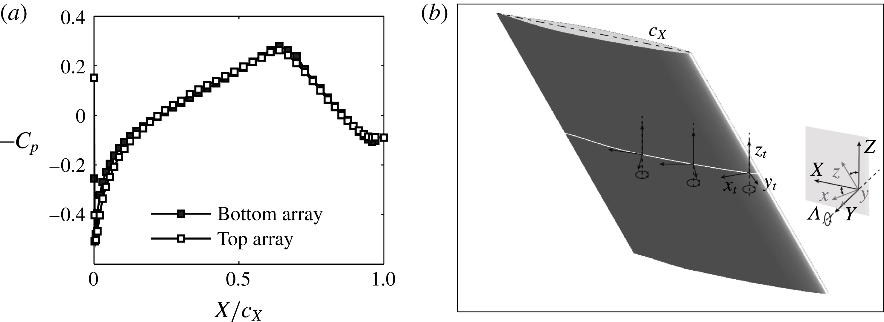
Reference Radeztsky, Reibert and Saric1999). The invariance of the flow along the leading edge direction is assessed by two arrays of 46 pressure taps placed near the two wing ends (300 mm from the tunnel walls). At
 $\unicode[STIX]{x1D6FC}=3^{\circ }$
, the flow shows a high degree of uniformity when checking the pressure distributions of the two arrays (see figure 1
a). Furthermore it is worth noticing that, for this flow configuration, the measured pressure minimum point is at
 $X/c_{X}=0.63$
thus ensuring a fully stable boundary layer with respect to Tollmien–Schlichting (TS) modes.
(a) Pressure distribution on the wing pressure side measured by two arrays of 46 pressure taps placed 300 mm from the top and bottom wing tips respectively at
 $\unicode[STIX]{x1D6FC}=3^{\circ }$
and
 $Re=2.17\times 10^{6}$
. (b) Schematic of the model and definition of the
 $xyz$
,
 $XYZ$
and
 $x_{t}y_{t}z_{t}$
reference systems.

Due to the inherent complexity of the geometry and flow topology, several reference systems are introduced. These are presented in figure 1(b). Firstly, the unswept coordinate system is defined with the upper case letters
 $XYZ$
and is positioned such that the
 $X$
and
 $Y$
axes lie in a horizontal plane (
 $X$
being in the chord plane and
 $Y$
orthogonal to that plane) while the
 $Z$
is the vertical direction. The velocity components along this coordinate system are indicated with upper case letters
 $UVW$
. The wing is rotated at incidence angle of
 $\unicode[STIX]{x1D6FC}=3^{\circ }$
and, as such, the wind tunnel reference system does not coincide with the unswept wing coordinates. The velocity components along the wind tunnel reference systems are denoted with upper case letters and the subscript:
 $_{\infty }$
.
The swept reference system is such that its
 $x$
axis is orthogonal to the wing leading edge, the
 $z$
axis is parallel to the leading edge (both these axes belong to the chord plane) and the
 $y$
axis coincides with the unswept
 $Y$
direction. By rotating the
 $XYZ$
system about the
 $Y$
axis by
 $\unicode[STIX]{x1D6EC}=45^{\circ }$
, one goes to the swept
 $xyz$
system. The velocity components in this system of coordinates are indicated with the lower case letters
 $uvw$
.
A last coordinate system needs to be introduced as the local tangential system (the definition of tangential is simplified here as it implies only the surface curvature along the
 $X$
direction). This system is positioned such that its
 $x_{t}$
axis is along the surface tangent, the
 $y_{t}$
is the wall-normal direction and
 $z_{t}$
coincides with the
 $Z$
axis.
2.2 AC-DBD plasma actuators
As identified earlier, for the needs of this study, actuator-induced roughness is of great importance. To this end, special actuators were designed, built and employed. The actuators were manufactured using a metal deposition technique developed in-house. The technique makes use of computer-controlled spraying of sub-micron conductive silver particles on the dielectric surface. The resulting electrode thickness is of the order of 1
 $\unicode[STIX]{x03BC}\text{m}$
. For comparison, traditional hand-made actuators based on adhesive copper tape, typically have electrode thickness of 60
 $\unicode[STIX]{x03BC}\text{m}$
. The plasma actuators were placed at
 $x/c=0.025$
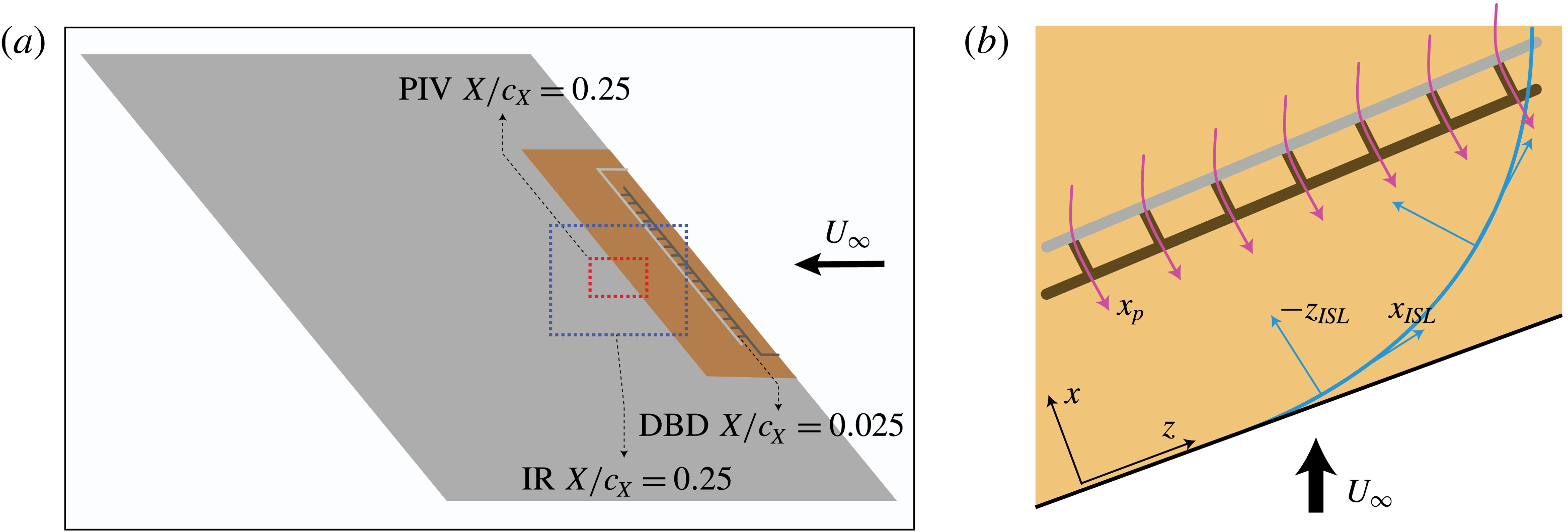
, close to the primary mode critical station (see the LST analysis of § 3). The plasma actuators were designed towards forcing a single monochromatic primary cross-flow mode. To force the desired mode, the employed actuators feature one straight electrode, which is exposed to the flow and is powered by the high-voltage supply. The grounded electrode is encapsulated below the dielectric barrier and is made of a series of stems spaced equally from each other and oriented along
 $x$
(see figure 3
b). The spacing between the stems defines the spanwise wavelength of the plasma forcing, and as such the spanwise wavelength of the forced CF modes. Three different modes were forced in this study, namely
 $\unicode[STIX]{x1D706}_{z}=9$
mm, which corresponds to critical mode (Serpieri & Kotsonis Reference Serpieri and Kotsonis2016), and
 $\unicode[STIX]{x1D706}_{z}=7$
mm and
 $\unicode[STIX]{x1D706}_{z}=12$
mm, corresponding to sub-critical and super-critical modes respectively.
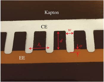
A detail of the DBD plasma actuators used in this study is presented in figure 2. The covered electrode stems are
 $d=10$
mm long and
 $w=3$
mm wide. They are projected towards the straight electrode overlapping with it by
 $o=2$
mm, in order to ensure consistent plasma formation. Given the relative large length of these stems, the flow ionisation region corresponds only to the electrode overlapping area thus ensuring the desired spanwise modulation of the forced jet. It is important to note that the exposed electrode was placed downstream so as to have the induced jet aligned with
 $-x$
(see figure 3
b).
Kapton polyimide film of 50
 $\unicode[STIX]{x03BC}\text{m}$
thickness was used as dielectric barrier. A second layer of Kapton was placed between the actuator and the model surface to better protect the latter. As such, the total thickness of the actuator was measured to be 125
 $\unicode[STIX]{x03BC}\text{m}$
. In order to avoid exposure of the incoming flow to a step of such high thickness, the Kapton sheet was wrapped around the wing leading edge. This ensured that the only surface perturbation seen by the flow was a two-dimensional backward facing step of 125
 $\unicode[STIX]{x03BC}\text{m}$
at approximately 10 % of the model chord. Preliminary investigations, using PIV and infrared thermography, indicated no adverse effects on the transition location by the physical presence of the actuator on the wing.
Detail (picture) of a DBD plasma actuator used for selective forcing of monochromatic primary cross-flow instability modes. The Kapton sheet, the covered electrode (CE), the exposed electrode (EE), the stems wavelength (
 $\unicode[STIX]{x1D706}_{z}$
), the width (
 $w$
), the distance between the electrodes (
 $d$
) and the overlap (
 $o$
) are also shown. View of the underside of the actuator, CE on foreground, EE on background.

(a) Schematic of the wind tunnel model with the actuators (Kapton sheet in orange, CE in dark grey, EE in light grey). Definition of the field of view of the IR thermography (blue dashed rectangle) and of the PIV (red dashed rectangle) experiments. (b) Schematic of the plasma actuator. The plasma jets (magenta), the inviscid streamline (cyan) and the related reference system (ISL) are shown together with the swept reference system (
 $xz$
). The schematics are not to scale.

The actuator was powered using a Trek 20/20C HS high-speed high-voltage amplifier. Depending on the case, the actuation signal was sinusoidal with amplitudes (E) between 2 and 3 kV. The scope of this study is to prove the applicability of DBD plasma actuators as control devices to condition the spanwise wavelength of primary cross-flow instability modes. As such, the high-voltage signal frequency (carrier frequency) was chosen considering the development of unsteady instability modes in the boundary layer. Preliminary linear stability theory analysis (presented in § 3) showed that the considered boundary layer is unstable to travelling primary instability modes comprised in the band 0–1 kHz. Therefore for the main tested cases, the actuators were operated at 2 kHz. To decouple the effects of unsteady forcing from the effects of forcing monochromatic CFI modes, a two-dimensional spanwise-uniform actuator was also considered.
2.3 Infrared thermography
The boundary layer transition evolution was inspected by IR thermography. The model was irradiated by two 1 kW halogen lamps placed approximately one metre from the model. The convective heat flux from the wing surface to the flow is a function of the local wall shear. As such, regions of high shear cool more rapidly than respective low shear regions. Differences in wall temperature captured by the thermal camera can therefore be used for visualisation between laminar and turbulent regions (see also Saric, Carpenter & Reed Reference Saric, Carpenter and Reed2011). In addition, using highly sensitive, actively cooled thermal imagers, details in the shear distribution of laminar boundary layers, such as the characteristic streaky footprint of CFVs can be retrieved.
The set-up for the IR thermography experiment is presented in the schematic of figure 4(a). The camera was mounted at about 1 m distance from the model surface and placed outside the wind tunnel, looking through an opportune germanium window. The imaged field of view was
 $480\times 360~\text{mm}^{2}$
and centred at
 $X/c_{X}=0.25$
,
 $Z=0$
(see the schematic of figure 3(a), where the IR domain is shown with a dashed (blue) rectangle). The IR camera used for the current experiment was a CEDIP Titanium 530L, featuring a mercury–cadmium–telluride quantum sensor with
 $320\times 256~\text{px}^{2}$
. The sensor is actively cooled by means of a Stirling cycle to the working temperature of 77 K resulting in a noise equivalent temperature difference of less than 18 mK. The integration time and the operated frame rates were 200
 $\unicode[STIX]{x03BC}\text{s}$
and 100 Hz respectively. The camera was equipped with a 25 mm focal length germanium lens operated at
 $f_{\sharp }=2.0$
.
Schematics (not to scale) of the experimental set-ups. The flow comes from right. The model (in black), the testing chamber (semi-transparent) and the opportune diagnostics windows are shown. (a) IR-thermography experiment with the IR camera (in brown). (b) High-speed PIV experiment with the PIV camera (in blue), the laser head (in dark green) and the light sheet from downstream (light green).

2.4 Particle image velocimetry
Particle image velocimetry was performed towards quantification of the boundary layer velocity field. Planar high-speed PIV was chosen for this experiment. The inspected planes are along the
 $X-Z$
directions at a distance of 1.5 mm from the model surface. The planes are centred with the station
 $X/c_{X}=0.25-Z=0$
of the model (see the schematic of figure 3(a), where the PIV domain is shown with a dashed (red) rectangle).
The PIV experimental set-up is presented in figure 4(b). As shown, the camera was imaging the field of view (FOV) from outside the wind tunnel through available optical windows and was placed at approximately 1 m distance from the measured plane. The camera used in this experiment is a LaVision Imager HS featuring a sensor of
 $2016\times 2016~\text{px}^{2}$
and pixel size of 11
 $\unicode[STIX]{x03BC}\text{m}$
and 12 bits of digital resolution. The active image sensor was reduced to
 $1632\times 496~\text{px}^{2}$
for the current experiment. The imager was equipped with a Nikon Nikkor 200 mm micro lens operated at
 $f_{\sharp }=5.6$
. The resulting magnification factor of the PIV experiment is
 $M=0.24$
. Illumination was provided from downstream as shown in the schematic of figure 4(b). A Nd:YAG high-speed Continuum Mesa PIV laser (18 mJ pulse
 $^{-1}$
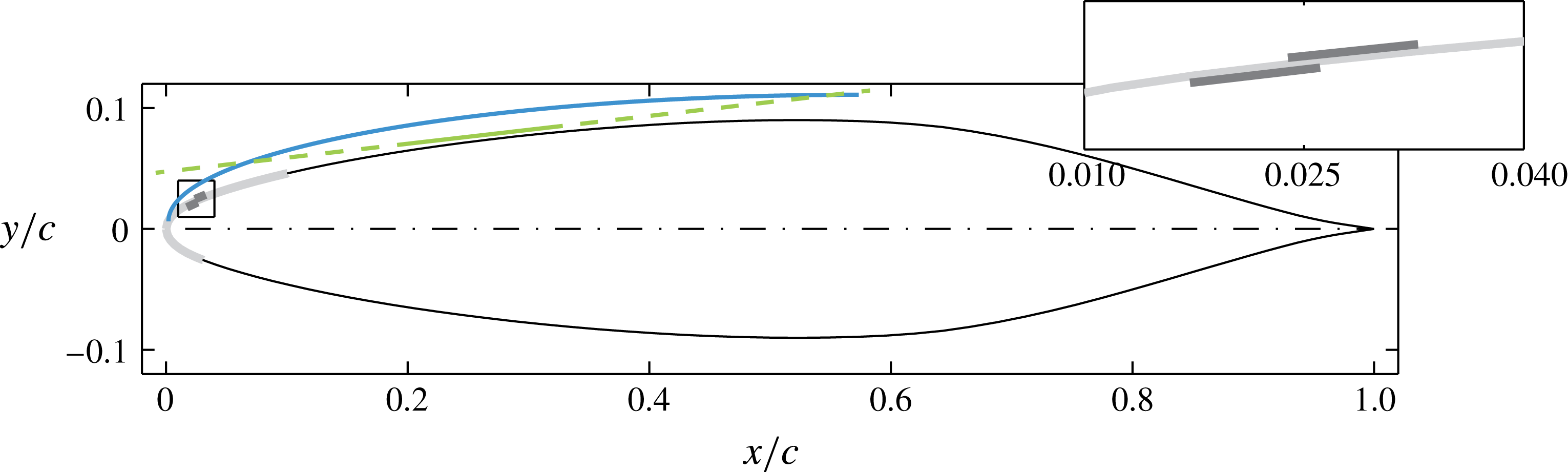
) was employed for particle illumination. The light beam was opportunely shaped into a sheet of approximately 1 mm thickness. The light sheet was oriented so as to be parallel to the model surface for all the imaged domain as shown in figure 5. In the schematic the AC-DBD plasma actuator is also shown. The Kapton sheet is in light grey and the electrodes in dark grey. Note that this is the wing cross-section orthogonal to the leading edge direction.
Wing section and schematic (not to scale) of the laser light (light green) and of the boundary layer (cyan). The AC-DBD plasma actuator is also shown: Kapton sheet in light grey; electrodes in dark grey. Inset: magnified view of the actuator. The wing section is orthogonal to the leading edge.

The flow was seeded using Safex water glycol injected downstream of the testing chamber. The average particle diameter is 1
 $\unicode[STIX]{x03BC}\text{m}$
. Synchronisation of the system was guaranteed by using the LaVision Davis 8.2 suite and a LaVision High Speed Controller unit. Image acquisition, pre-processing and correlation were performed with the same software. Cross-correlation was performed with final interrogation windows of
 $24\times 24~\text{px}^{2}$
with relative overlap set to 75 %. As such the final vector spacing was approximately 0.27 mm in both
 $X$
and
 $Z$
. The time interval between the two laser pulses was set to 15
 $\unicode[STIX]{x03BC}\text{s}$
so as to give an average particle displacement in the free stream of 15 px. The measurement frame rate (FR) was 3000 Hz and sequences of 6000 image pairs were acquired, for every tested flow case. The resulting measurement time was 2 s.
The correlation random error in planar PIV is estimated to be 0.1 px (Raffel et al.
Reference Raffel, Willert, Wereley and Kompenhans2007). Therefore the random error, relative to the free stream velocity, is
 $\unicode[STIX]{x1D700}_{(U,V)}=0.1/15=0.007$
. This is also the measurement error for the statistic velocity fluctuations fields (
 $\{U_{t}^{\prime },V_{t}^{\prime }\}_{RMS}$
). Here
 $U_{t}^{\prime }$
and
 $V_{t}^{\prime }$
are the time velocity fluctuations (i.e. after subtracting the time average). The uncertainty on the time-averaged velocity fields is retrieved from the flow fluctuations magnitude, estimated to be less than 10 % of the free stream velocity, and from the measurement ensemble size (
 $ES$
):
 $\unicode[STIX]{x1D700}_{(\bar{U},\bar{V})}=0.1/\sqrt{ES}$
, where the overbar denotes time averaging. The ensemble size to be considered here does not encompass all the 6000 captured fields. These are correlated in time with respect to the travelling instability modes, which account for most of the fluctuation energy at the measurement location (Serpieri & Kotsonis Reference Serpieri and Kotsonis2016). The fluctuations related to this instability feature high energy content in the frequency band
 $100~\text{Hz}\leqslant f\leqslant 400~\text{Hz}$
(Serpieri & Kotsonis Reference Serpieri and Kotsonis2016). Therefore a conservative time sub-sampling of the measured fields is required in order to formally render them uncorrelated in time. This factor can be estimated as FR
 $/\text{min}(f_{(U_{t}^{\prime },V_{t}^{\prime })})=3000~\text{Hz}/100~\text{Hz}=30$
and is used to estimate the uncorrelated ensemble size as a fraction of the total of the captured samples:
 $ES_{u}=ES/30=200$
. Finally, the uncertainty on the time-averaged velocity fields can be evaluated as
 $\unicode[STIX]{x1D700}_{(\bar{U},\bar{V})}=0.1/\sqrt{ES_{u}}\approx 0.018$
.
2.5 Non-dimensionalisation and normalisation
Several reference systems and different experimental and numerical techniques were used and described in the present study. Part of the results is therefore presented in non-dimensional units. The airfoil chords along the
 $X$
and
 $x$
directions are used as reference length scales for the respective coordinate systems. However, some results are presented in dimensional units to ease comparison with dimensional quantities and avoid introduction of elaborated nomenclature. This consideration follows from the actuators employed in this study. These devices can be described by non-dimensional quantities as e.g. the momentum coefficient (see § 5). However, the main dimensional parameters, namely the frequency of the driving AC voltage and the wavelength of the electrodes, are crucial for the description and understanding of the presented analyses. The velocity scale used in the remainder is the free stream velocity (
 $U_{\infty }$
). In addition,
 $U_{\infty }^{2}$
is used to non-dimensionalise the velocity power spectra.
When specified, the presented spectra are normalised as shown in (2.1) (in agreement with Parseval’s theorem),
 $$\begin{eqnarray}\unicode[STIX]{x1D6F7}_{\unicode[STIX]{x1D6FE}}^{\ast }\cdot \unicode[STIX]{x1D6FF}_{f}=(\unicode[STIX]{x1D6F7}_{\unicode[STIX]{x1D6FE}}\cdot \unicode[STIX]{x1D6FF}_{f})\frac{\displaystyle \frac{1}{ES-1}\unicode[STIX]{x1D6F4}_{t}(\unicode[STIX]{x1D6FE}^{\prime })^{2}}{\unicode[STIX]{x1D6F4}_{f}(\unicode[STIX]{x1D6F7}_{\unicode[STIX]{x1D6FE}}\cdot \unicode[STIX]{x1D6FF}_{f})},\end{eqnarray}$$
where
 $\unicode[STIX]{x1D6F7}$
is the power spectral density (PSD),
 $\unicode[STIX]{x1D6FF}_{f}$
is the spectra frequency resolution,
 $\unicode[STIX]{x1D6FE}$
is the spectra variable and
 $ES$
the temporal ensemble size. The sums are performed with respect to the subscript quantity (i.e. time (
 $t$
) at the numerator and frequency (
 $f$
) at the denominator).
3 Stability of the laminar boundary layer
The stability of the laminar boundary layer is investigated by means of numerical solutions of the boundary layer equations and linear stability theory. In two-dimensional boundary layers, LST is a common tool to predict the early (linear) stages of instability growth (Schlichting & Gersten Reference Schlichting and Gersten2000). The extension to three-dimensional flows is straightforward if flow invariance along the leading edge direction is respected (Mack Reference Mack1984). This hypothesis reduces the flow around a swept wing to what is usually referred to as infinite swept wing flow or 2.5-dimensional flow. The formulation of the problem and description of the solver are presented in appendix A. Several investigations made use of LST either as design/validation tool for experimental investigations or as initial condition for parabolised stability equations (PSE) computations (e.g. Reibert et al. Reference Reibert, Saric, Carrillo and Chapman1996; Arnal et al. Reference Arnal, Gasparian and Salinas1998; Malik et al. Reference Malik, Li, Choudhari and Chang1999; Högberg & Henningson Reference Högberg and Henningson1998; Haynes & Reed Reference Haynes and Reed2000).
3.1 Formulation
The linear stability problem is presently solved using the Chebyshev spectral collocation method, with 100 polynomials. The spatial formulation is chosen where the flow disturbances are expressed in the waveform of (3.1),
 $$\begin{eqnarray}\unicode[STIX]{x1D713}(x,y,z,t)=\unicode[STIX]{x1D719}(y)\text{e}^{\text{i}(\unicode[STIX]{x1D6FC}x+\unicode[STIX]{x1D6FD}z-\unicode[STIX]{x1D714}t)},\end{eqnarray}$$
where
 $\unicode[STIX]{x1D714}$
(angular frequency) is real,
 $\unicode[STIX]{x1D6FC}$
(wavenumber along
 $x$
) is complex and
 $\unicode[STIX]{x1D6FD}$
(wavenumber along
 $z$
) is real as no growth is assumed along the
 $z$
direction based on the assumption of spanwise invariance.
Details on the derivation of the Orr–Sommerfeld (OS) equation for 2.5-dimensional flows are given by Mack (Reference Mack1984) (pp. 3–13). The companion matrix technique of Bridges & Morris (Reference Bridges and Morris1984) is employed to overcome the eigenvalue nonlinearity. N factors (
 $N$
) are computed as the integral of growth rates (i.e. the imaginary part of the chordwise wavenumbers:
 $-\unicode[STIX]{x1D6FC}_{i}$
) along
 $x$
. Envelope N factors (
 $N^{env}$
) are the
 $x$
-integral of the local maximum values, per chord station, among all the considered modes (i.e. wavenumbers) (Arnal et al.
Reference Arnal, Gasparian and Salinas1998; Serpieri & Kotsonis Reference Serpieri and Kotsonis2016). Equations (3.2a,b
) give the mathematical formulations of these two quantities,
 $$\begin{eqnarray}N(x,\unicode[STIX]{x1D706}_{z},\unicode[STIX]{x1D714})=\int _{x_{0}(\unicode[STIX]{x1D706}_{z},\unicode[STIX]{x1D714})}^{x}-\unicode[STIX]{x1D6FC}_{i}(\unicode[STIX]{x1D701},\unicode[STIX]{x1D706}_{z},\unicode[STIX]{x1D714})\,\text{d}\unicode[STIX]{x1D701};\quad N^{env}(x,\unicode[STIX]{x1D714})=\max |_{\unicode[STIX]{x1D706}_{z}}(N(x,\unicode[STIX]{x1D706}_{z},\unicode[STIX]{x1D714})).\end{eqnarray}$$
3.2 Results
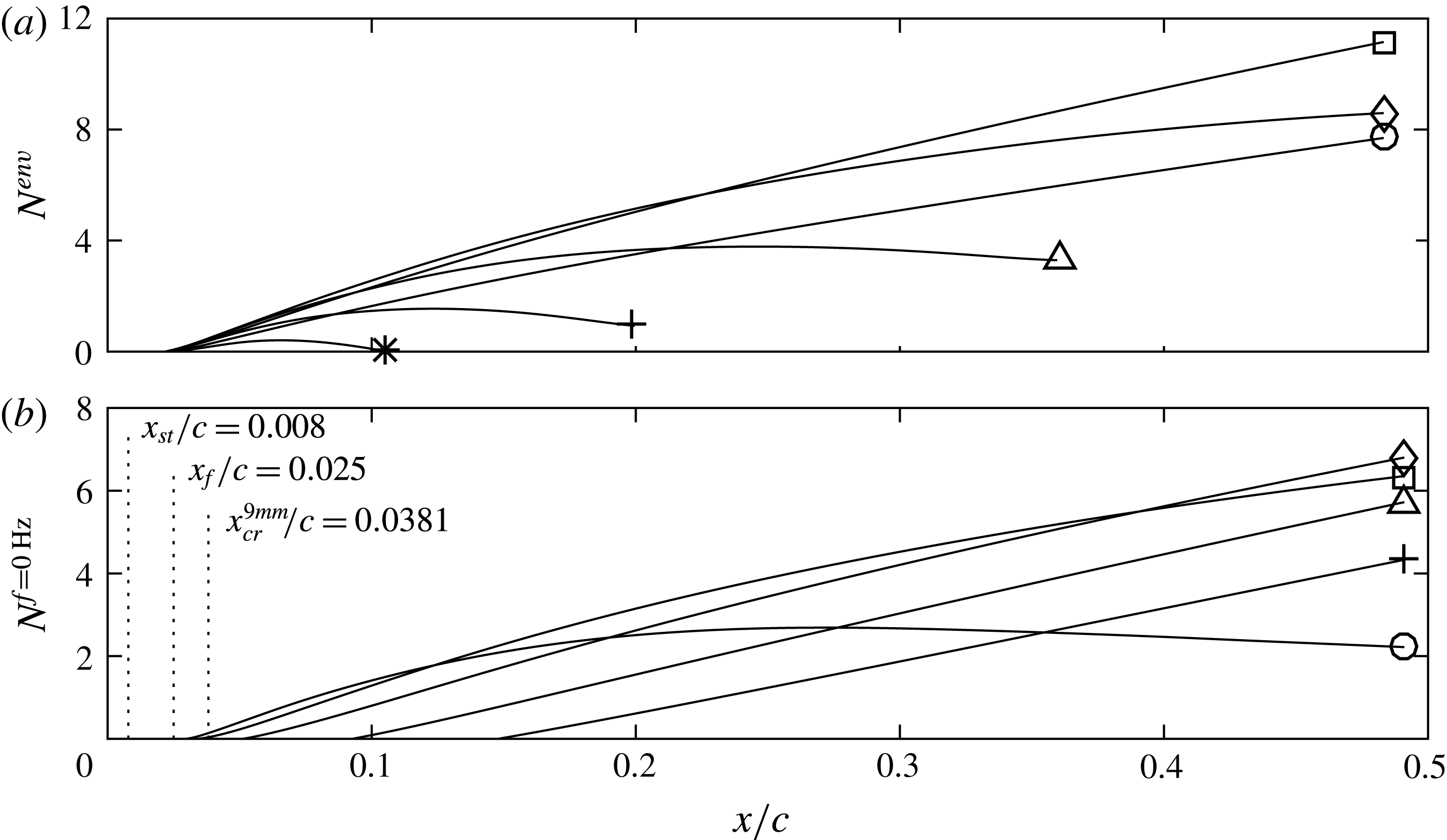
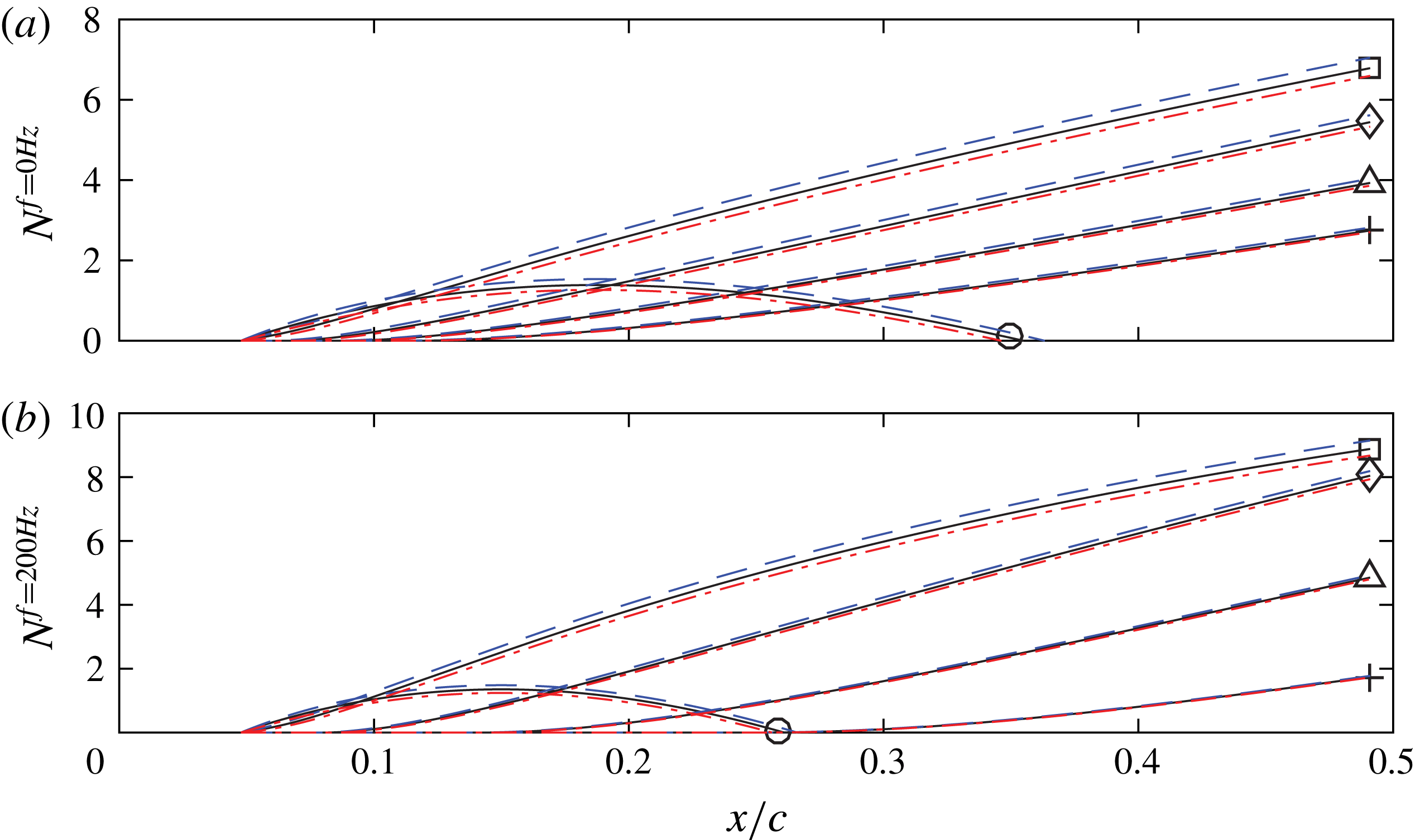
The comparison of envelope N factors, between stationary and travelling modes of various frequencies, is presented in figure 6(a). Modes in the
 $0~\text{Hz}\leqslant f\leqslant 600~\text{Hz}$
frequency band show strongest amplification close to the stagnation point. While the
 $f=600$
Hz mode saturates at
 $x/c\approx 0.21$
, the lower frequency waves are amplified throughout the boundary layer with the 200 Hz mode being the most amplified mode. The fact that steady modes have lower growth than the travelling waves is a common outcome of LST analyses (Malik et al.
Reference Malik, Li, Choudhari and Chang1999; Haynes & Reed Reference Haynes and Reed2000). Nevertheless, the eventual dominance of stationary modes over unsteady modes in practical cases is conditioned by the boundary layer receptivity to surface roughness and free stream turbulence, which is not accounted for in the LST eigenvalue problem. As such, while predicted by LST to be weaker, stationary vortices dominate the transition scenario in low turbulence flows (Deyhle & Bippes Reference Deyhle and Bippes1996).
Lastly, it is important to note that higher frequency modes are unstable only for shorter portions of the wing. For example, the
 $f=1000$
Hz mode is only weakly amplified near the leading edge and by station
 $x/c=0.113$
reaches
 $N^{env}=0$
. Modes with higher frequency are either less amplified or they never destabilise in the current conditions. These preliminary results serve as an initial handle towards choosing the forcing frequency of the used plasma actuators. Specifically, the LST results suggest that unsteady forcing should be applied at frequencies that are higher than the unstable band shown.
(a) Envelope N factors for different frequencies (○: 0 Hz; ▫: 200 Hz; ♢: 400 Hz; ▵: 600 Hz;
 $+$
: 800 Hz; *: 1000 Hz). (b) N factors of different stationary modes (○:
 $\unicode[STIX]{x1D706}_{z}=5$
mm; ▫:
 $\unicode[STIX]{x1D706}_{z}=7$
mm; ♢:
 $\unicode[STIX]{x1D706}_{z}=9$
mm; ▵:
 $\unicode[STIX]{x1D706}_{z}=12$
mm;
 $+$
:
 $\unicode[STIX]{x1D706}_{z}=15$
mm).
 $x_{st}$
indicates the stagnation point,
 $x_{f}$
is the forcing location and
 $x_{cr}^{9mm}$
is the critical station for the
 $\unicode[STIX]{x1D706}_{z}=9$
mm mode. See (3.2) for the formulation of the plotted quantities.

A comparison between stationary modes with different wavelengths is shown in figure 6(b). While in the most downstream regions the predicted instability is dominated by the
 $\unicode[STIX]{x1D706}_{z}=9$
mm mode (see also Serpieri & Kotsonis Reference Serpieri and Kotsonis2016), the smaller-wavelength modes are dominating upstream as a consequence of the lower local Reynolds number. The DRE/UFD flow control strategy pivots on this phenomenon. Selective forcing of stationary modes with smaller wavelengths with respect to the eventually most amplified one, delays the amplification of the latter and consequently postpones the flow breakdown (Saric et al.
Reference Saric, Carrillo and Reibert1998; Malik et al.
Reference Malik, Li, Choudhari and Chang1999; Wassermann & Kloker Reference Wassermann and Kloker2002). For the presently studied flow, a stationary mode with spanwise wavelengths in the range of
 $\unicode[STIX]{x1D706}_{z}=5{-}7$
mm should lead to these beneficial effects. The location of the stagnation point
 $x_{st}$
, of the actuators
 $x_{f}$
and the critical location for the
 $\unicode[STIX]{x1D706}_{z}=9$
mm (
 $x_{cr}^{9mm}$
) are also plotted.
It must be noted here that LST gives only indications of the pertinent modes evolution as it does not account for non-parallel and nonlinear effects. Furthermore, it does not account for the disturbances initial amplitude (i.e. the receptivity problem). Finally, neither the boundary layer nor the OS equation solver account for the model curvature and flow non-parallel effects. The effect of these parameters has been thoroughly analysed by Haynes & Reed (Reference Haynes and Reed2000). Nonetheless, the outcomes discussed here give valuable information for the design of the employed flow control devices.
4 Test cases
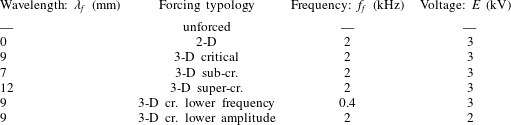
Six forced flow cases are analysed in this study in addition to the unforced flow case. The first case corresponds to two-dimensional uniform forcing, enabled by a spanwise-invariant actuator. This is followed by three spanwise-modulated forcing cases at critical (
 $\unicode[STIX]{x1D706}_{f}=9$
mm), sub-critical (
 $\unicode[STIX]{x1D706}_{f}=7$
mm) and super-critical (
 $\unicode[STIX]{x1D706}_{f}=12$
mm) wavelengths. Notwithstanding the forced mode, the actuators were installed at identical locations (
 $x_{f}/c=0.025$
). The actuators were supplied with a sinusoidal signal at
 $f_{f}=2$
kHz and with voltage amplitude of
 $E=3$
kV (i.e. voltage peak to peak of 6 kV). The choice for the forcing frequency was based on the considerations in § 5.1. More specifically, the frequency was chosen to be 2 kHz so as to lie considerably above the LST-predicted unstable CFI band of
 $0<f<1000$
Hz. In addition to the aforementioned cases a low frequency and low amplitude case were considered. For the low frequency case, the voltage amplitude is kept to
 $E=3$
kV but the frequency is reduced to 400 Hz thus in the range of the amplified primary CFI (§ 3). For the low amplitude case, a signal of reduced voltage (
 $E=2$
kV) and same frequency (2 kHz) was inspected in order to elucidate the amplitude effects. The two additional cases were considered only for the critical wavelength actuator (
 $\unicode[STIX]{x1D706}_{f}=9$
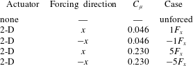
mm). The parameters of the tested cases are summarised in table 1.
Tested flow cases.

5 Actuator characterisation
In this section, the mechanical performance of the used actuators is quantified. The spanwise-uniform 2-D actuator is chosen for this analysis, simplifying the flow field to a two-dimensional arrangement. The identified amplitude effects are expected to reasonably describe the performance of the spanwise-modulated actuators, considering that their electrode width (
 $w$
) remains constant. The characterisation is carried out in quiescent flow. Planar high-speed PIV was employed to measure the induced velocity and compute the actuator body-force and the related thrust (for details on the body-force extraction methods see Kotsonis et al. (Reference Kotsonis, Ghaemi, Veldhuis and Scarano2011) and Kotsonis (Reference Kotsonis2015)). Furthermore, spectral analysis of the unsteady flow field is presented to infer the unsteady flow field induced by the actuators.
5.1 Experimental set-up
The camera, laser and synchronisation equipment used for this experiment are the same as described in § 2.4. For this experiment, the camera’s active sensor was reduced to
 $960\times 440~\text{px}^{2}$
to increase its maximum frame rate. The camera was equipped with a Nikon Nikkor 200 mm macro lens operated at
 $f_{\#}=8$
. The magnification factor was
 $M=1.14$
. The air in the closed box was seeded with droplets of paraffin oil,
 $1~\unicode[STIX]{x03BC}\text{m}$
in average diameter, generated by a TSI Atomizer nozzle. The coordinate system used in this experiment is represented by the symbols
 $x_{p}y_{p}z_{p}$
(see figure 3
b). The system is arranged such that the
 $x_{p}$
axis is in the direction of the induced jet (i.e. orthogonal to the electrodes length), the
 $y_{p}$
is perpendicular to the plane of the actuator and
 $z_{p}$
is along the length of the electrodes. The plasma actuator was installed in a transparent acrylic glass box enclosing a volume of
 $0.25~\text{m}^{3}$
(1 m long along
 $x_{p}$
). The plane inspected with PIV is aligned with
 $x_{p}-y_{p}$
, given the uniformity of the induced flow field along
 $z_{p}$
. The laser, camera and transparent box were installed on a pneumatically stabilised table (i.e. an optical table) to avoid vibrations on the set-up which could be detrimental for such high magnification planar PIV experiment. Cross-correlation was carried out with final interrogation windows of
 $24\times 24~\text{px}^{2}$
with relative overlap set to
 $75\,\%$
. As such, the final vector spacing was approximately 0.053 mm in both
 $x_{p}$
and
 $y_{p}$
directions. The system was operated at acquisition rate of 10 kHz in single-frame mode thus the pulse separation between the correlated frames was
 $100~\unicode[STIX]{x03BC}\text{s}$
. Sequences of 25 000 images were acquired for each test case for a total measurement time of 2.5 s. The measurement started prior to plasma actuation thus capturing the initial flow acceleration phase.
5.2 Performance
In quiescent flow environments, when the actuator is supplied with the voltage signal, the strong electric field established between the electrodes ionises and accelerates the air molecules. The incompressible Navier–Stokes momentum equation is used to retrieve the induced body force. In this very initial regime, advection, diffusion and pressure terms are negligible with respect to the unsteady acceleration and body-force terms. Following Kotsonis et al. (Reference Kotsonis, Ghaemi, Veldhuis and Scarano2011), under the specified assumptions, the momentum equation reduces to
 $\boldsymbol{F}=\unicode[STIX]{x1D71A}$
 $\unicode[STIX]{x2202}\boldsymbol{U}/\unicode[STIX]{x2202}t$
, where
 $\boldsymbol{F}$
is the body force and
 $\boldsymbol{U}$
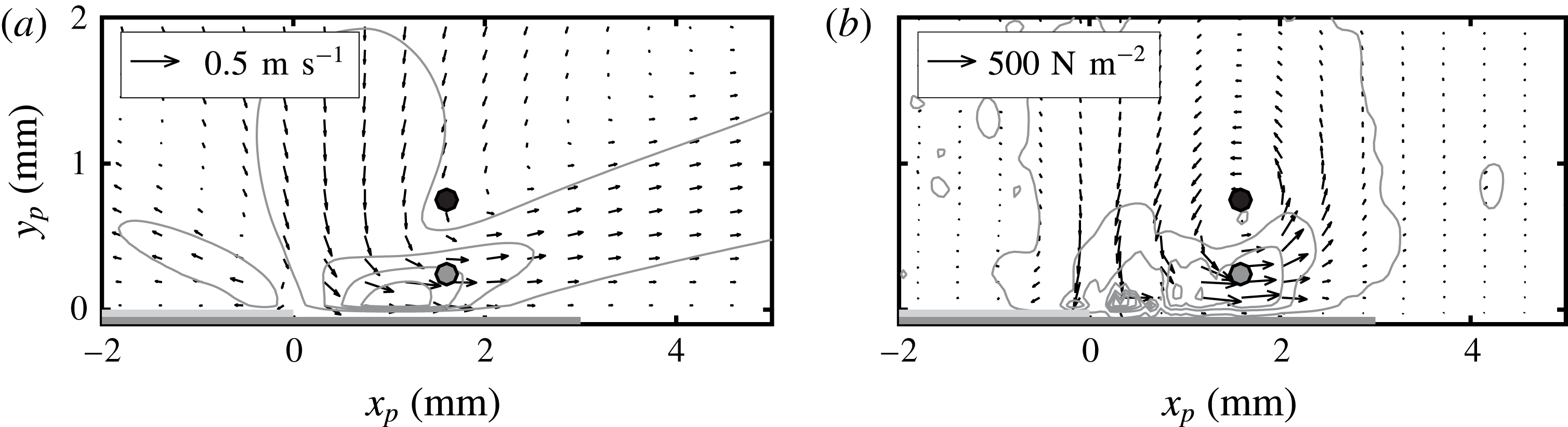
the velocity. Low-pass filtering of the measured velocity signal was applied in order to eliminate high frequency oscillations associated with the AC voltage frequency. In addition to the body forces, the time-averaged velocity field is computed, after the induced jet has fully developed, from the measured time series and presented in figure 7 for the case of
 $f_{f}=2~\text{kHz}-E=3~\text{kV}$
.
The induced jet originates in the vicinity of the inner edge of the exposed electrode and is mainly aligned with the
 $x_{p}$
direction. The wall-normal velocity component, at the electrodes interface, supplies the mass for the wall-parallel jet (Kotsonis et al.
Reference Kotsonis, Ghaemi, Veldhuis and Scarano2011). A secondary wall-parallel jet, oriented opposite to the main velocity, is observed on top of the exposed electrode. This secondary jet is not observed with the usual copper electrode actuators and can be caused by the extremely low thickness of the employed actuators building up a competing electrical field. A confined region of negative
 $x_{p}$
-body force is also observed. The body-force field is overall rather weak, for the tested conditions, and predominant along the
 $x_{p}$
direction (Kotsonis Reference Kotsonis2015).
(a) Time-averaged velocity magnitude field (grey solid lines: 5 levels, from 0 to
 $0.6~\text{m}~\text{s}^{-1}$
). (b) Body-force magnitude field (grey solid lines: 5 levels, from 50 to
 $1000~\text{N}~\text{m}^{-2}$
). Vectors:
 $x_{p}-y_{p}$
components of the respective contour variables (reference vector in the upper left corner). AC-DBD actuator operated at
 $f_{f}=2~\text{kHz}-E=3~\text{kV}$
. The two horizontal grey lines below
 $y_{p}=0$
represent (to scale) the electrodes of the actuator. The markers at
 $x_{p}=1.6~\text{mm}-y_{p}=0.25$
(grey) and 0.75 mm (black) refer to figure 8.

Spatial integration of the body-force field retrieves the exerted specific (i.e. per actuator unit length) thrust. This is eventually used to compute the momentum coefficient, according to (5.1), which is used to compare the actuators authority for the different forcing conditions,
 $$\begin{eqnarray}C_{\unicode[STIX]{x1D707}}=\frac{T_{x_{p}}}{\frac{1}{2}\unicode[STIX]{x1D71A}{u_{e}}^{2}\unicode[STIX]{x1D717}_{u}},\end{eqnarray}$$
where the local (at the actuator position) boundary layer edge velocity
 $u_{e}=14~\text{m}~\text{s}^{-1}$
and momentum thickness
 $\unicode[STIX]{x1D717}_{u}=7.81\times 10^{-2}$
mm are extracted from the boundary layer numerical solution for the investigated case (see appendix A).
The thrust generated by the plasma actuator along
 $x_{p}$
and the respective momentum coefficient for the different test cases considered in this study are presented in table 2. When the actuator is operated at
 $f_{f}=2~\text{kHz}-E=3$
kV, the horizontal component of the thrust generated is
 $T_{x_{p}}=0.432~\text{mN}/m_{act}$
and the momentum coefficient is
 $C_{\unicode[STIX]{x1D707}}=0.046$
. This is the combination of supplied voltage and frequency that leads to the strongest induced jet. When the frequency is reduced to 400 Hz, the performance of the actuator is reduced. Similarly, decreasing the voltage amplitude to 2 kV at the same operated frequency of 2 kHz, lowers
 $C_{\unicode[STIX]{x1D707}}$
.
For all the investigated configurations of table 2, the generated thrust is comparatively less than what reported by Chernyshev et al. (Reference Chernyshev, Kuryachii, Manuilovich, Rusyanov and Skvortsov2013) and Dörr & Kloker (Reference Dörr and Kloker2015b ) in their studies. However, in the current study, the AC-DBD plasma jets are used in a respective fashion to isolated roughness elements for DRE/UFD flow control. In such a configuration, the actuators are used to induce a weak localised perturbation of the incoming flow thus requiring only moderate forcing amplitudes. The specific thrust applied by the actuators used by Dörr & Kloker (Reference Dörr and Kloker2017) for the same purpose is comparable to the values reported here.
AC-DBD actuator-induced thrust and momentum coefficient.

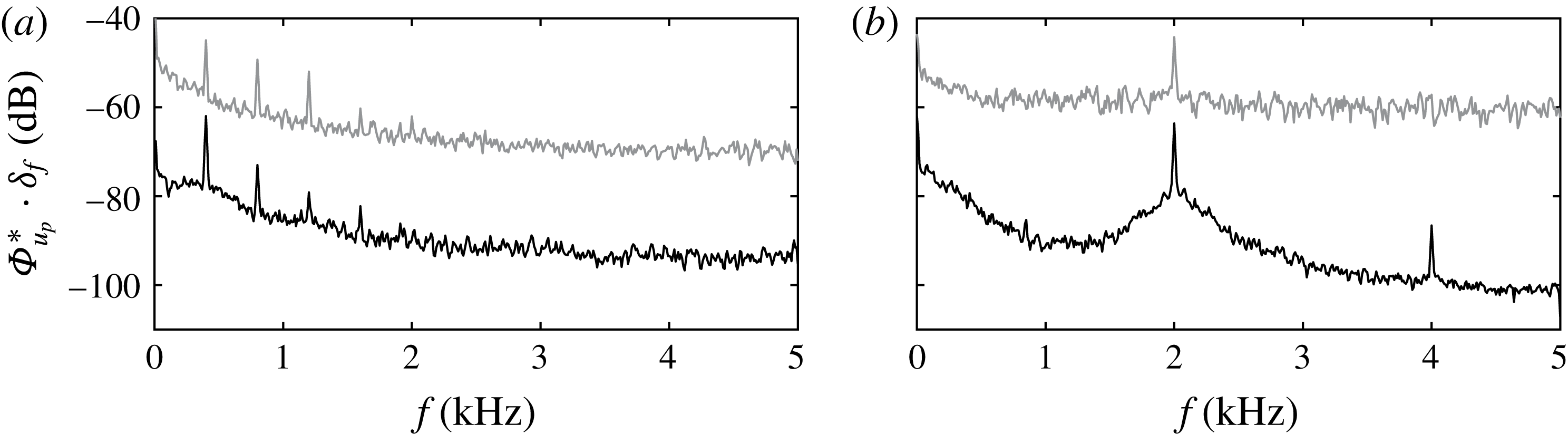
Capitalising on the high sampling rate of the employed PIV method, access to the unsteady and spectral features of the plasma-induced flow field is gained. Spectral analysis of the velocity fluctuations, at two points at
 $x_{p}=1.6~\text{mm}-y_{p}=0.25$
, 0.75 mm (markers in figure 7
a), was carried out for the two different frequencies at which the actuators were operated (0.4 and 2 kHz). The results are shown in figure 8. The spectra are normalised according to (2.1) and non-dimensionalised with
 $U_{\infty }^{2}$
thus they directly show the relative kinetic energy per frequency band. They reveal strong unsteady fluctuations at the respective carrier frequency as well as higher harmonics. Moreover, low frequency fluctuations close to the wall are observed. These can be attributed to a range of factors including plasma-induced thermal disturbances, measurement noise and unstable plasma formations. The exact origin of these fluctuations should be taken into account in the future for a complete characterisation of the plasma effect. Moreover, it is currently unclear to what extent these low frequency fluctuations would be present also on the wing mounted configuration under external flow condition. Such study will require a dedicated effort that goes beyond the scope of this article.
6 Infrared flow visualisation
In this section, flow visualisation results using IR thermography are presented. The IR fields will be used to inspect the effectiveness of the developed actuators in conditioning the stationary CFI modes. For all discussed results, geometrical mapping of the captured images was applied to account for the curvature of the model and the perspective effects from the camera.
Non-dimensional normalised power spectra of the actuators induced velocity
 $u_{p}$
(
 $\unicode[STIX]{x1D6F7}_{u_{p}}^{\ast }\cdot \unicode[STIX]{x1D6FF}_{f}/U_{\infty }^{2}$
, see (2.1),
 $\unicode[STIX]{x1D6FF}_{f}=10$
Hz) at the position of the markers (
 $x_{p}=1.6~\text{mm}-y_{p}=0.25$
(grey) and 0.75 mm (black)) in figure 7 (grey curve displaced by
 $+10$
dB for visualisation). (a)
 $f_{f}=0.4~\text{kHz}-E=3$
kV, (b)
 $f_{f}=2~\text{kHz}-E=3$
kV.

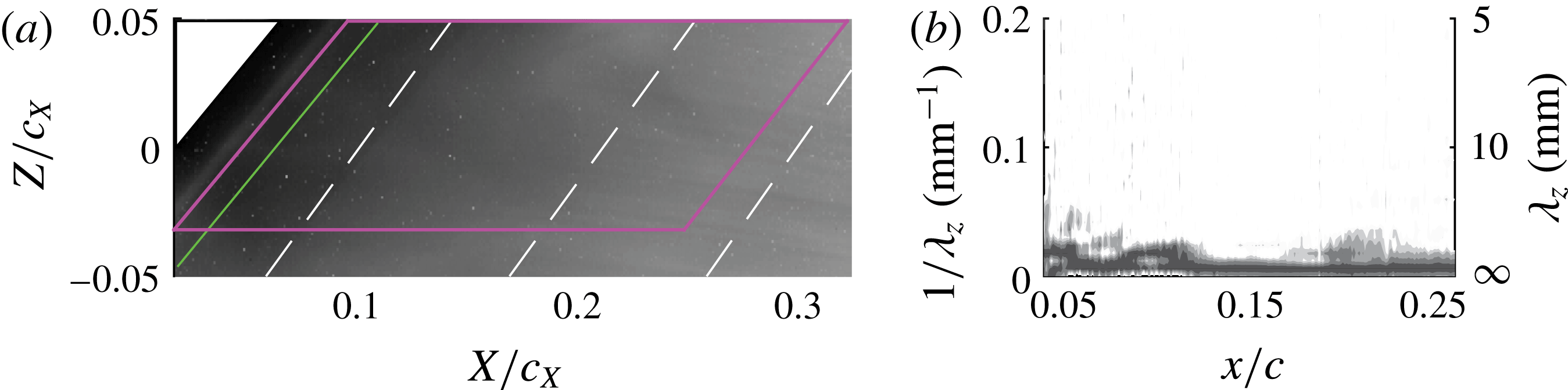
The IR flow visualisation for the natural transition flow (i.e. with no boundary layer forcing) is presented in figure 9(a). To enhance the signal-to-noise ratio of the measurements, time averaging of the captured thermography fields was performed over the sampled period (300 samples). The flow shows strong homogeneity in both the spanwise and chordwise directions. For the considered model (i.e. geometry and surface roughness), angle of attack, Reynolds number and free stream turbulence level, no strong CFI modes are amplified in the inspected range and the boundary layer remains laminar until the most downstream station inspected. To further analyse the spatial and spectral arrangement of the boundary layer from the IR image, the individual pixel intensities within the solid (magenta) lines depicted in figure 9(a) were sampled and analysed in the wavenumber spectral domain. This procedure was performed along constant chord lines. The power spectral density (
 $\unicode[STIX]{x1D6F7}$
) was computed using Welch’s algorithm (Welch Reference Welch1967). The wavenumber resolution of the spectra is
 $0.006~\text{mm}^{-1}$
. The results are presented in figure 9(b). No stationary modes appear above the measurement noise level for the unforced flow case.
Natural transition flow case. (a) IR thermography fields. The flow comes from left. The solid (green) line divides the figure in two regions where different contrast levels are used. The dashed white lines are constant-chord lines at
 $x/c=0.1$
, 0.2 and 0.3. The region enclosed with the solid (magenta) lines refers to figure 9(b). (b) Wavenumber power spectral density of the IR pixels intensity along the chord. The analysis is performed in the region within the solid (magenta) lines of figure 9(a).

The IR fields for the four actuators operated at
 $f_{f}=2~\text{kHz}-E=3$
kV (
 $C_{\unicode[STIX]{x1D707}}=0.046$
) are shown in figure 10. The plasma regions initiated by the actuators are clearly visible in the images close to the leading edge as localised regions of increased thermal radiation. This is mainly attributed to a weak heating effect of the model surface directly beneath the plasma formation as reported by Kotsonis (Reference Kotsonis2015). In the case of spanwise-uniform forcing (figure 10
a), the plasma manifests as a bright continuous line in the
 $z$
direction. When the spanwise-modulated forcing is applied (figure 10
b–d), the localised plasma regions spaced at the respective forced wavelength appear as a sequence of bright spots. Due to the high IR intensity of the plasma formation, intensity equalisation (de-saturation) has been applied to facilitate observation of IR intensity distribution downstream of the actuators (the solid (green) line in the fields divide the images in two regions with different contrast settings).
IR thermography fields. Actuators operated at
 $f_{f}=2~\text{kHz}-E=3$
kV (
 $C_{\unicode[STIX]{x1D707}}=0.046$
): (a) spanwise-uniform forcing; (b) sub-critical forcing (
 $\unicode[STIX]{x1D706}_{f}=7$
mm); (c) critical forcing (
 $\unicode[STIX]{x1D706}_{f}=9$
mm); (d) super-critical forcing (
 $\unicode[STIX]{x1D706}_{f}=12$
mm). The regions enclosed with the solid (magenta) lines refer to figure 11.

For the two-dimensional forcing, the flow does not exhibit significant alteration of the stationary vortices, compared to the unforced case. Eventually, moving more downstream, stationary waves do take place, however their intensity and spacing appear uneven along lines parallel to the leading edge. No clear transition fronts, within the imaged FOV are evident in this flow case. When spanwise-modulated forcing is applied, the thermal footprint of primary instability modes becomes more visible in the IR fields. The resulting streaks appear locked to the spacing and the position of the plasma regions. Their relative intensity is also more uniform along constant-chord lines, further suggesting conditioning of both wavelength and amplitude of the stationary cross-flow vortices by the plasma actuator. Overall, for the spanwise-modulated forcing, a more uniform flow topology is established with evident monochromatic structures present in the more upstream portion of the wing. Additionally, in figure 10(b,d) the appearance of turbulent wedges at the most downstream portions of the FOV suggests advancement of the transition front due to actuation.
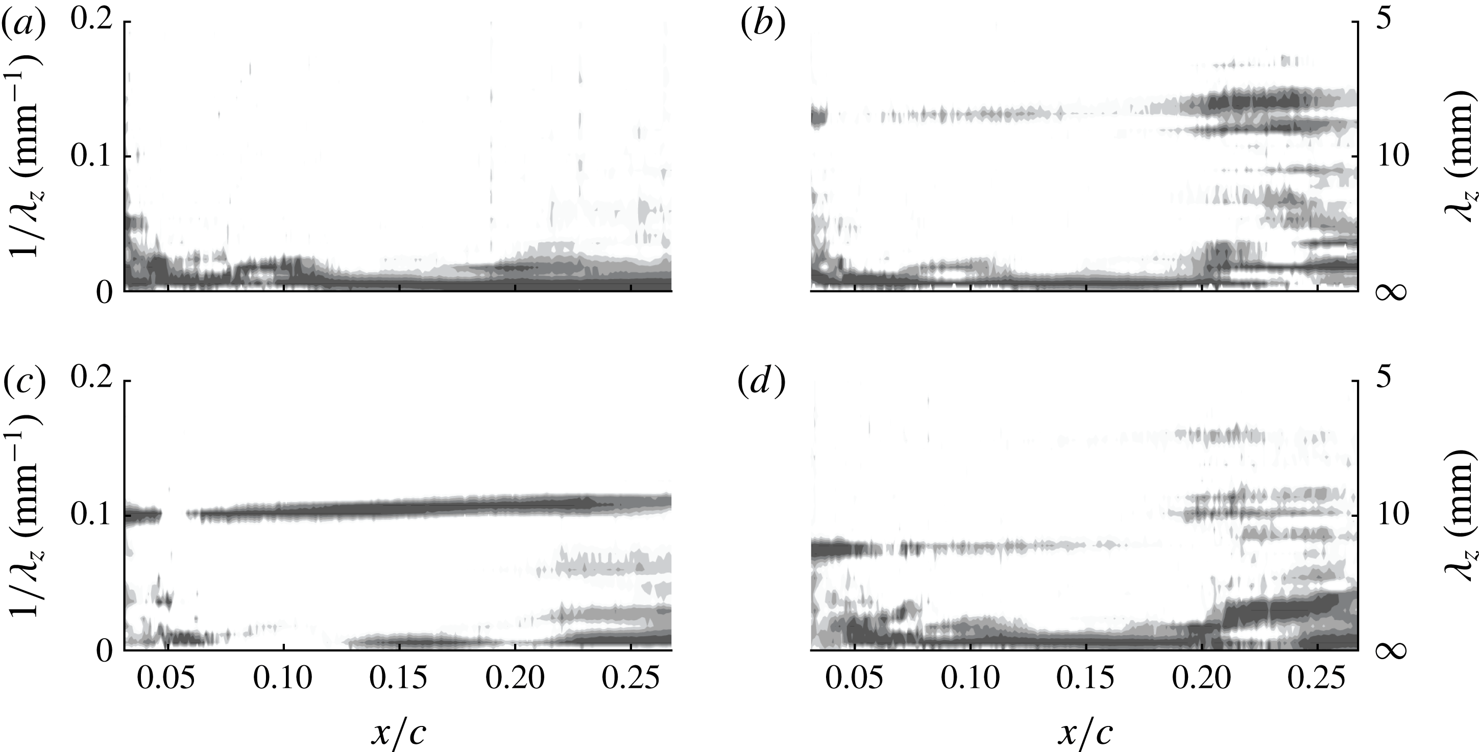
Wavenumber power spectral density of the IR pixels intensity along the chord. Same cases as figure 10.

The IR pixels intensity spectra for the flow cases of figure 10 are presented in figure 11. When spanwise-uniform forcing is applied, no dominating stationary modes are present in the upstream portion of the FOV similar to the unforced flow case of figure 9. In the most downstream region, the spectrum shows weak energy levels corresponding to the development of some coherent streaks as shown in figure 10(a). When spanwise modulated forcing is applied, the wavenumber spectra reveal the presence of harmonic peaks closely aligned to the forced wavelength. Comparing the spectra of figure 11(b–d) to the respective IR images in figure 10(b–d) it becomes apparent that the selective forcing at the plasma wavelength effectively conditions the formation of the stationary cross-flow vortices at approximately the same wavelength. This is especially evident for the
 $\unicode[STIX]{x1D706}_{f}=7$
mm and 9 mm actuators fields. Moreover, it is shown that the critical mode (
 $\unicode[STIX]{x1D706}_{z}=9$
mm) is the most receptive to leading edge forcing, showing the highest spectral energy levels throughout the inspected domain. When the sub-critical
 $\unicode[STIX]{x1D706}_{z}=7$
mm waves are forced (figure 11
b), the most downstream portion of the domain shows a much broader spectrum with longer wavelengths modes being amplified. Finally, when the
 $\unicode[STIX]{x1D706}_{z}=12$
mm mode is forced (figure 11
d), stationary waves at the forced wavelength are amplified. From
 $x=0.19c$
, a super-harmonic mode with double wavenumber (wavelength of
 ${\approx}6.1$
mm) is also captured. Amplification of superharmonic modes is a commonly observed feature in CFI boundary layers (Reibert et al.
Reference Reibert, Saric, Carrillo and Chapman1996) related to nonlinear interaction between primary modes (Haynes & Reed Reference Haynes and Reed2000). Energy at wavelengths of 10 mm and 9 mm is also captured downstream of
 $x=0.19c$
.
Wavenumber power spectral density of the IR pixels intensity along the chord.
 $\unicode[STIX]{x1D706}_{f}=9$
mm actuator operated at: (a)
 $f_{f}=0.4~\text{kHz}-E=3$
kV (
 $C_{\unicode[STIX]{x1D707}}=0.013$
); (b)
 $f_{f}=2~\text{kHz}-E=2$
kV (
 $C_{\unicode[STIX]{x1D707}}=0.037$
).

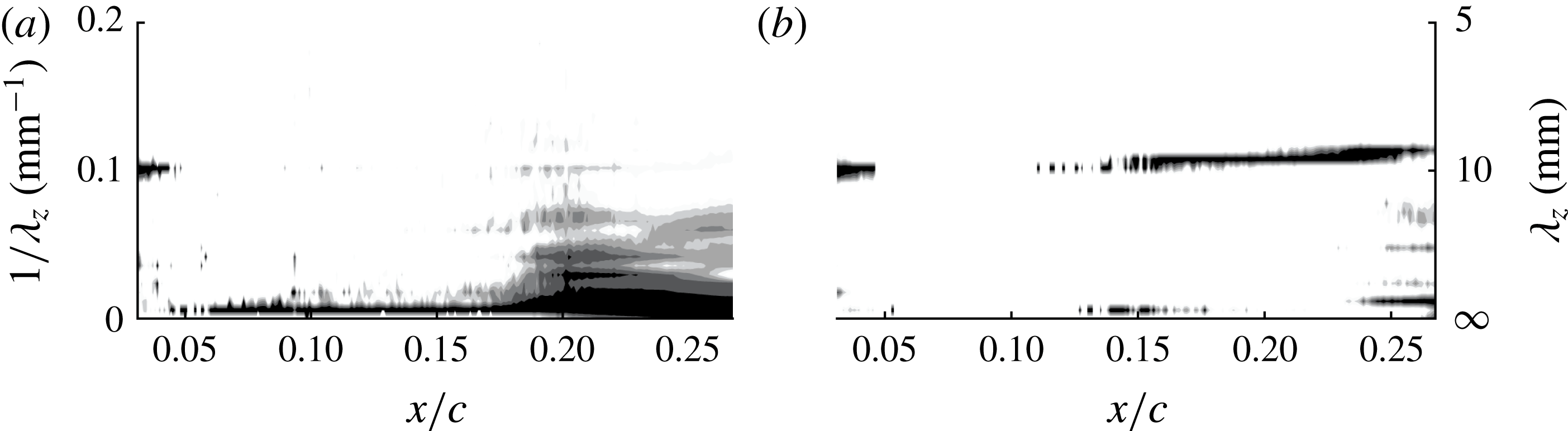
The wavenumber spectra equivalent to those presented in figure 11 are presented in figure 12 for the spanwise-modulated actuator of
 $\unicode[STIX]{x1D706}_{f}=9$
mm operated at the lower (400 Hz) frequency and at the lower voltage (2 kV). When the actuator is operated at
 $E=3~\text{kV}-f_{f}=400$
Hz (
 $C_{\unicode[STIX]{x1D707}}=0.013$
) (figure 12
a), spectral energy at the forced wavelength (9 mm) is weakly observed only in the range
 $0.18\leqslant x/c\leqslant =0.22$
, however this mode does not dominate the boundary layer and longer-wavelength modes are strongly amplified. The apparent weakness of the spectral coherence in this case is attributed to the frequency of the applied forcing, which falls in the band of the primary travelling modes as predicted by LST (figure 6
a). In these conditions, the eventual presence of strongly amplified unsteady vortices dominate over the stationary CFI. Furthermore, at these operational parameters, the momentum coefficient of the actuator (table 2) attains the lowest values among the tested cases. For the
 $E=2~\text{kV}-f_{f}=2$
Hz (
 $C_{\unicode[STIX]{x1D707}}=0.037$
) case (figure 12
b), the spectrum replicates similar features of the
 $E=3~\text{kV}-f_{f}=2~\text{Hz}$
(
 $C_{\unicode[STIX]{x1D707}}=0.046$
) case (see figure 11
c) albeit with lower energy levels. This indicates the possibility of adjusting the forcing amplitude of the actuators by tuning the supplied voltage, corroborating the observations of Schuele et al. (Reference Schuele, Corke and Matlis2013) (further analysed in the remainder).
7 Velocity field
In this section, the results of the high-speed PIV investigations are presented. The effect of the plasma forcing on the primary instability is quantified by means of the velocity field statistics. The spatio-temporal evolution of the unsteady flow field is further elucidated through spectral and proper orthogonal decomposition (POD) analyses.
7.1 Time-averaged flow topology
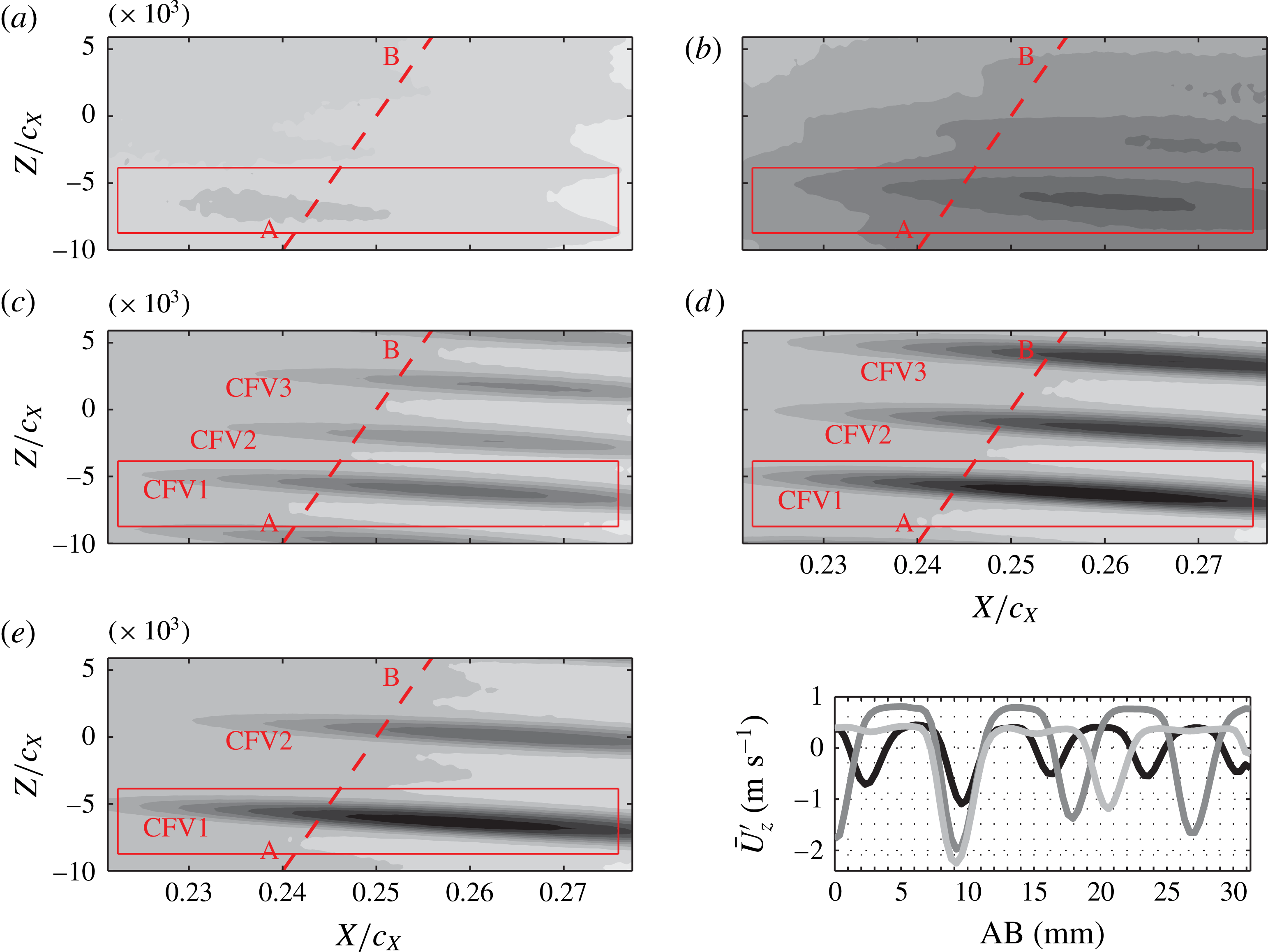
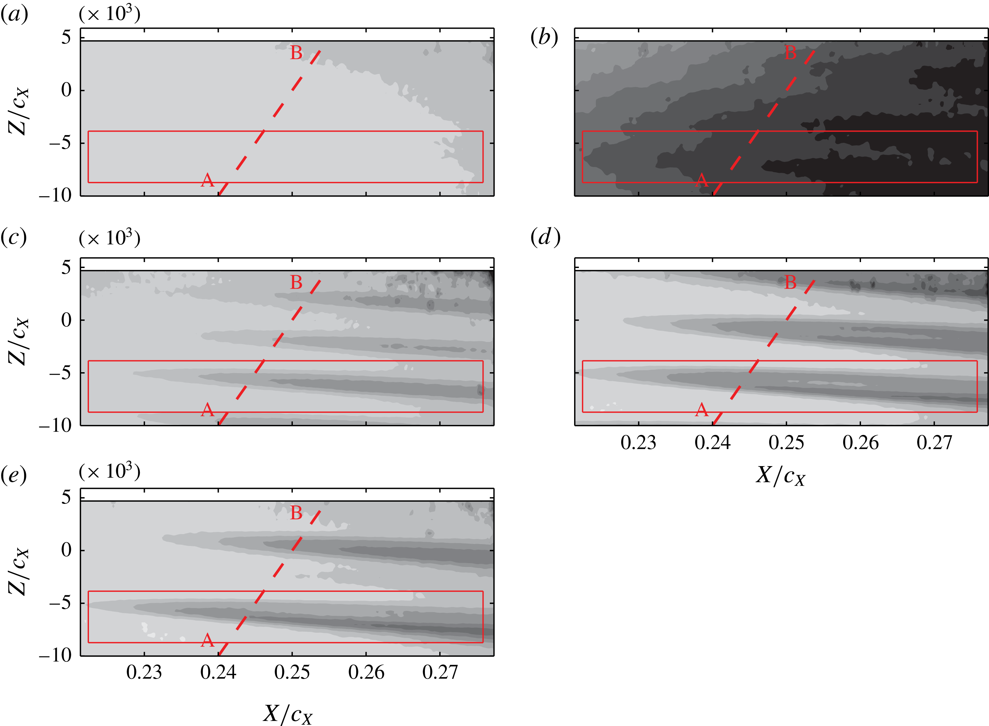
The time-averaged
 $U$
velocity fields for the different test cases are presented in figure 13. Figure 13(a) shows the unforced flow. The actuator is mounted on the wing but is not supplied with voltage. The boundary layer, within the imaged domain, is still laminar and slightly modified by natural CFI mechanisms as seen in figure 9(a). The appearance of stationary vortices is observed in the presented velocity field as a weak velocity modulation along the span.
Time-averaged
 $U$
velocity fields (10 levels, from 0.84 (black) to
 $1U_{\infty }$
(white)). The flow comes from left. (a) Actuator non-operated; (b) spanwise-uniform forcing; (c) sub-critical forcing (
 $\unicode[STIX]{x1D706}_{f}=7$
mm); (d) critical forcing (
 $\unicode[STIX]{x1D706}_{f}=9$
mm); (e) super-critical forcing (
 $\unicode[STIX]{x1D706}_{f}=12$
mm). Actuator operated at
 $f_{f}=2~\text{kHz}-E=3$
kV (
 $C_{\unicode[STIX]{x1D707}}=0.046$
). The (red) lines and labels refer to analyses presented in the remainder. Inset: spanwise fluctuation of the
 $\bar{U}_{z}^{\prime }$
velocity signal sampled along the line AB in fields: (c) black, (d) dark grey, (e) light grey line.

When two-dimensional forcing is applied (figure 13
b), the flow drastically rearranges. The overall magnitude of velocity is reduced, showing a thickening of the boundary layer. Moreover, the velocity local minima are now more distinguishable, suggesting the enhancement of the stationary primary vortices. When spanwise-modulated forcing is applied (figure 13
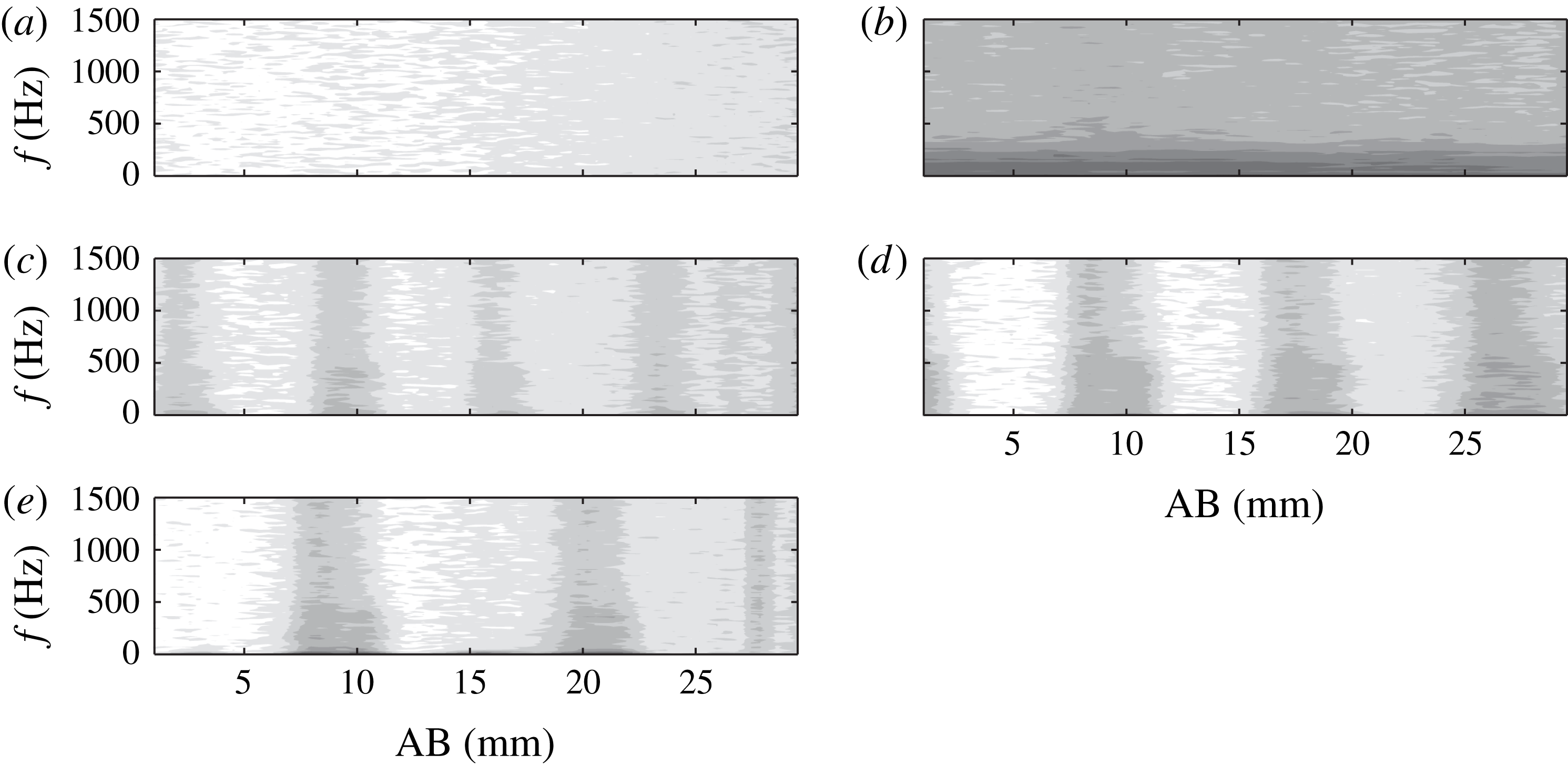
c–e), separate and more uniform stationary vortices become clearly visible. The spanwise spacing, along a line parallel to the leading edge (segment AB in the contours) can be compared to the actuated wavelength. The velocity spanwise fluctuations (
 $\bar{U}_{z}^{\prime }$
) for the spanwise-modulated flow cases are presented in the inset of figure 13, further reconciling with the outcomes of the flow visualisation experiment of § 6. When the super-critical mode (
 $\unicode[STIX]{x1D706}_{f}=12$
mm) is forced, the superharmonic mode seen before in figure 11(c) becomes evident, downstream of
 $x/c=0.25$
, in the regions in between the stronger CFVs. The lower side of the presented flow fields always shows lower velocities in comparison to the upper region. This effect is attributed to a possible small inclination of the laser sheet (i.e. rotation about the
 $X$
axis), such that the lower illuminated region is slightly closer to the wall.
Inspecting the fields pertaining to the three different forced wavelengths shows that, when critical forcing is applied, the vortices appear more developed than the sub-critical and super-critical forcing cases. In fact it can be seen that the velocity minima corresponding to the low-momentum region attain the lowest values for the
 $\unicode[STIX]{x1D706}_{z}=9$
mm vortices. In addition, the spatial evolution of the stationary waves can be quantified by computing their amplitude as defined by equation (7.1) (White & Saric Reference White and Saric2005 and Serpieri & Kotsonis Reference Serpieri and Kotsonis2016),
 $$\begin{eqnarray}A^{CFV}(x)=z_{rms}\{\bar{U_{z}^{\prime }}(x)/U_{\infty }\}|_{y_{t}=y_{t}^{PIV}}.\end{eqnarray}$$


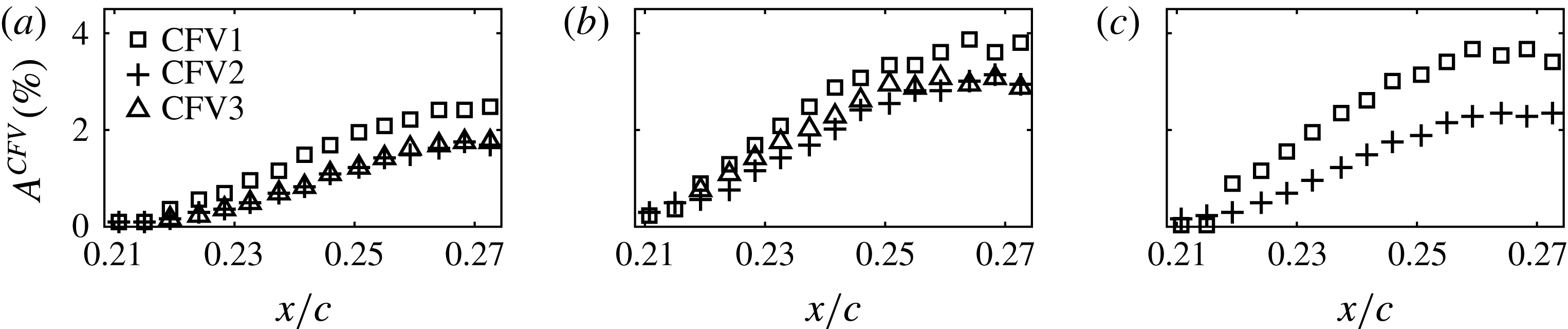
As evident in figure 13, ensembles of two to three individual vortices are available through the PIV measurements. Due to the fixed FOV, the number of fully resolved vortices is dependent on the forcing wavelength. For the calculation of the amplitudes, the individual vortices are tracked in their spatial evolution. The estimated amplitudes for the individual vortices in the spanwise-modulated forcing cases (figure 13 c–e) are shown in figure 14(a–c) respectively.
Within the imaged field, the stationary vortices show similar growths despite the different amplitudes. Forcing the critical mode at
 $\unicode[STIX]{x1D706}_{f}=9$
mm leads to more developed waves compared to the other two modes, especially with respect to the sub-critical mode, in both initial amplitude and spatial amplification. These results, which match with the stronger energy shown for this mode in the IR spectra (figure 11), confirm that forcing sub-critical modes leads to less amplified stationary vortices (see e.g. Reibert et al.
Reference Reibert, Saric, Carrillo and Chapman1996; Malik et al.
Reference Malik, Li, Choudhari and Chang1999 and Wassermann & Kloker Reference Wassermann and Kloker2002). All the fields show monotonic growth of the stationary vortices. However, the amplitudes appear to saturate at the most downstream portion of the fields. This is expected from boundary layers dominated by stationary CFVs undergoing laminar-to-turbulent transition (Haynes & Reed Reference Haynes and Reed2000; Serpieri & Kotsonis Reference Serpieri and Kotsonis2016). However, it has to be clarified here that performing this analysis on planes at constant distance from the model wall has some limitations. In fact, moving downstream, the stationary waves grow and so does the boundary layer (see the schematic of figure 5). Hence, moving downstream at a constant wall-normal position, the measurement plane intersects the stationary vortices in a lower region where the velocity modulation effect is milder. This results, when using the metrics of (7.1), in lower amplitudes. Therefore the growth rates of the stationary CF vortices should be retrieved from full three-dimensional fields (Reibert et al.
Reference Reibert, Saric, Carrillo and Chapman1996; Haynes & Reed Reference Haynes and Reed2000; Wassermann & Kloker Reference Wassermann and Kloker2002; White & Saric Reference White and Saric2005; Serpieri & Kotsonis Reference Serpieri and Kotsonis2016). Despite these observations, the effect is rather mild within small chordwise domains, such as the one considered here.
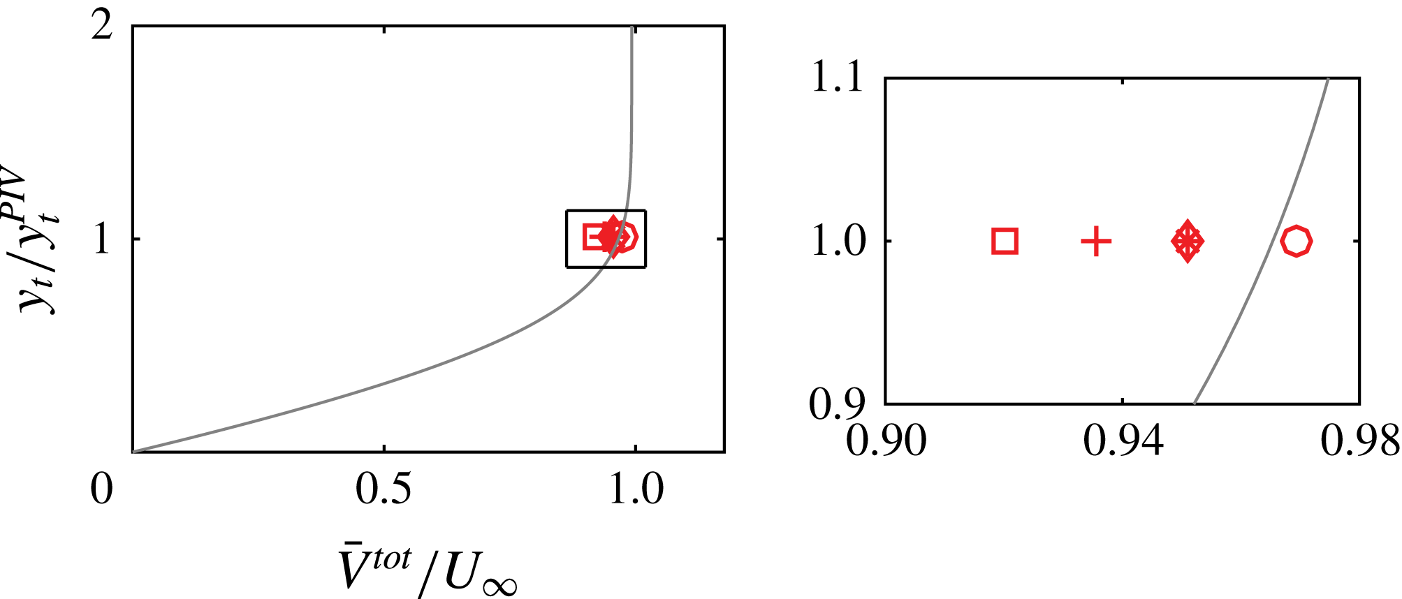
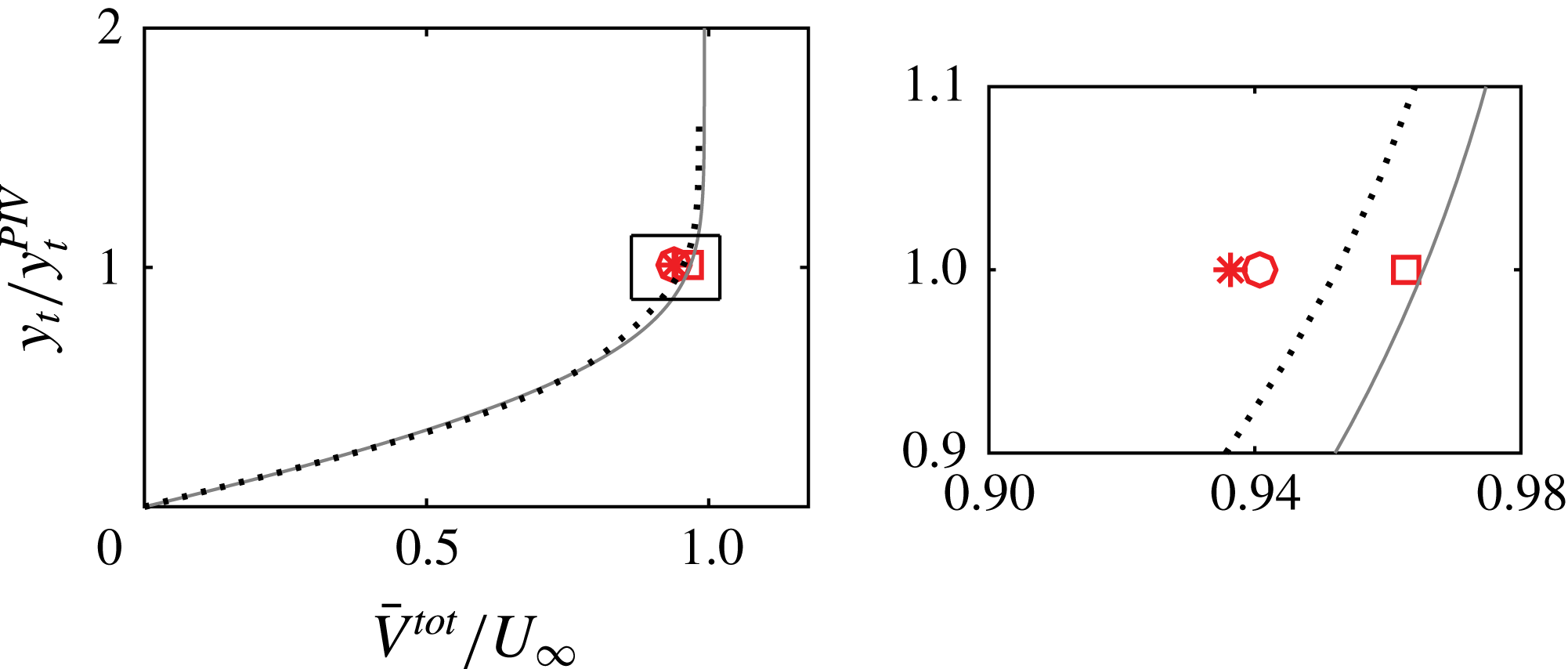
Comparison between the measured spanwise-mean velocity magnitude (
 $z_{mean}\{\bar{V}^{tot}\}|_{y_{t}=y_{t}^{PIV}}$
) from the velocity fields of figure 13 (symbols) and the boundary layer numerical solution (solid line) at
 $x/c=0.25$
. (○) Actuator non-operated; (▫) spanwise-uniform forcing; (*) sub-critical forcing (
 $\unicode[STIX]{x1D706}_{f}=7$
mm); (
 $+$
) critical forcing (
 $\unicode[STIX]{x1D706}_{f}=9$
mm); (♢) super-critical forcing (
 $\unicode[STIX]{x1D706}_{f}=12$
mm). Inset: magnified view.

An additional consideration in the analysis of figure 14 relates to the fact that the mean-flow distortion of the considered fields caused by the primary CFVs is not even. In fact, more developed vortices modify the mean flow more significantly. A way to inspect this effect is proposed here by comparing the measured spanwise-mean velocity magnitude (
 $z_{mean}\{\bar{V}^{tot}\}|_{y_{t}=y_{t}^{PIV}}$
) from the velocity fields of figure 13 (sampled along the AB segment) and the undisturbed boundary layer numerical solution (described in appendix A). The outcomes of this comparison are presented in figure 15. Evidently, the boundary layer corresponding to the spanwise-uniform and spanwise-modulated critically forced (
 $\unicode[STIX]{x1D706}_{f}=9$
mm) flows underwent significant mean-flow distortion. The unforced flow case as well as the super-critical (
 $\unicode[STIX]{x1D706}_{f}=12$
mm) and sub-critical (
 $\unicode[STIX]{x1D706}_{f}=7$
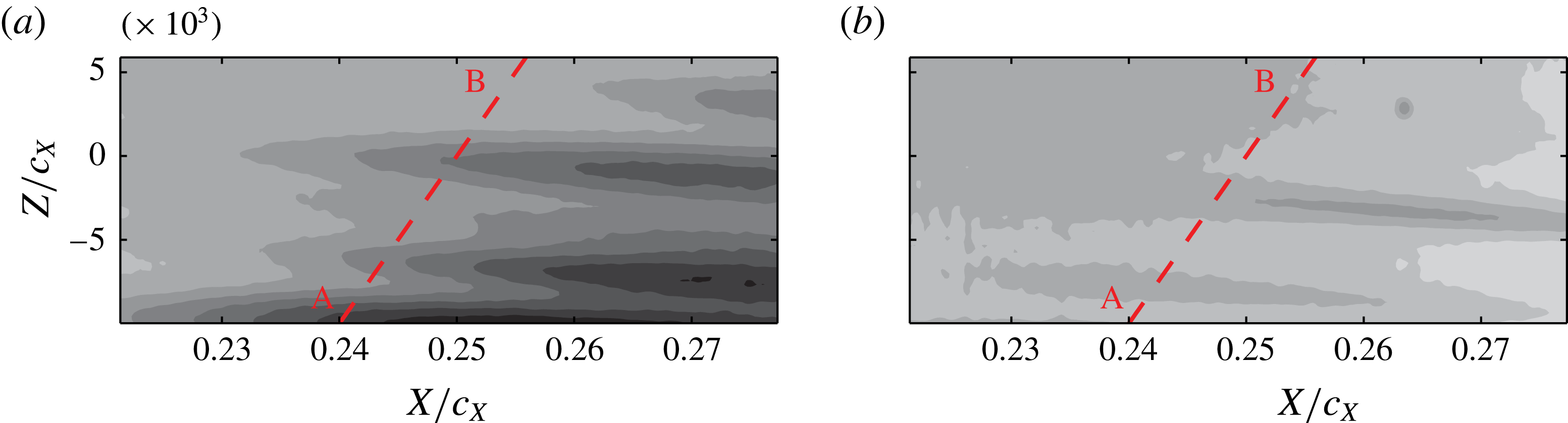
mm) forcing cases are distorted more mildly. The measured unforced boundary layer agrees relatively well with the numerical prediction. The slight discrepancy is attributed to modelling assumptions in the boundary layer solution as well as measurement uncertainties in the PIV fields.
Time-averaged
 $U$
velocity fields (10 levels, from 0.84 (black) to
 $1U_{\infty }$
(white)). (a)
 $f_{f}=0.4~\text{kHz}-E=3$
kV (
 $C_{\unicode[STIX]{x1D707}}=0.013$
); (b)
 $f_{f}=2~\text{kHz}-E=2~\text{kV}$
(
 $C_{\unicode[STIX]{x1D707}}=0.037$
).

The time-averaged velocity field for the additional forcing case of the critical mode actuator operated at the lower frequency (400 Hz) and same voltage amplitude (3 kV,
 $C_{\unicode[STIX]{x1D707}}=0.013$
) is presented in figure 16(a). The velocity field shows a spanwise modulation with amplified stationary vortices at different wavelengths. When the actuator is operated at
 $f_{f}=2~\text{kHz}-E=2~\text{kV}$
(
 $C_{\unicode[STIX]{x1D707}}=0.037$
) (figure 16
b), the boundary layer features weaker stationary vortices when compared to the
 $f_{f}=2~\text{kHz}-E=3$
kV case (figure 13
d). This further confirms the dependency of forced cross-flow vortex strength to the momentum coefficient of the actuator.
A comparison of the present study to the passive control investigation of Serpieri & Kotsonis (Reference Serpieri and Kotsonis2016), is shown in figure 17. In this previous work, the critical cross-flow instability mode was conditioned with leading edge micron-sized roughness elements (diameter:
 $d_{r}=2.8$
mm, height:
 $k_{r}=10~\unicode[STIX]{x03BC}\text{m}$
) installed at the same chordwise position as the plasma actuators in the present study (
 $x/c=0.025$
). The velocity profile was acquired with hot-wire scans. Note that the velocity measured in that experiment, coincides mainly with
 $\sqrt{U^{2}+V^{2}}$
, however, given the strong predominance of the
 $U$
component (Serpieri & Kotsonis Reference Serpieri and Kotsonis2016), this comparison can still be valid. The comparison demonstrates that, when the actuator is operated at
 $f_{f}=2~\text{kHz}-E=3~\text{kV}$
(
 $C_{\unicode[STIX]{x1D707}}=0.046$
), the spanwise-averaged value of the mean velocity attains the lowest value among all cases. For the lower frequency case, the lower velocity value compared to the laminar solution is explained by the more advanced transitional status of the forced boundary layer. When the actuator was operated at 400 Hz, the boundary layer showed multiple stationary modes (figure 12
a) and enhanced fluctuations (see the discussion of figure 20
a). Moving to the other flow cases, the comparison with the passive roughness elements used by Serpieri & Kotsonis (Reference Serpieri and Kotsonis2016) is more instructive given the CFI monochromatic state of the compared boundary layers. The hot-wire profile shows already at this chordwise station a small deviation from the laminar profile, caused by the mean-flow distortion (Serpieri & Kotsonis Reference Serpieri and Kotsonis2016). Moreover, the profile crosses the station of the current PIV measurements (
 $y_{t}=1.5$
mm) between the velocity values of the tested voltages thus showing that the
 $d_{r}=2.8~\text{mm}-k_{r}=10~\unicode[STIX]{x03BC}\text{m}$
passive roughness has a milder effect on the boundary layer than the
 $f_{f}=2~\text{kHz}-E=3~\text{kV}$
(
 $C_{\unicode[STIX]{x1D707}}=0.046$
) active roughness but stronger compared to the
 $f_{f}=2~\text{kHz}-E=2~\text{kV}$
(
 $C_{\unicode[STIX]{x1D707}}=0.037$
) case.
Comparison between the measured spanwise-mean velocity magnitude (
 $z_{mean}\{\bar{V}^{tot}\}|_{y_{t}=y_{t}^{PIV}}$
) from the velocity fields of figure 16 (symbols), the boundary layer numerical solution (solid line) at
 $x/c=0.25$
. Critical forcing (
 $\unicode[STIX]{x1D706}_{f}=9$
mm): (○)
 $f_{f}=0.4~\text{kHz}-E=3$
kV (
 $C_{\unicode[STIX]{x1D707}}=0.013$
); (▫)
 $f_{f}=2~\text{kHz}-E=2$
kV (
 $C_{\unicode[STIX]{x1D707}}=0.037$
); (*)
 $f_{f}=2~\text{kHz}-E=3$
kV (
 $C_{\unicode[STIX]{x1D707}}=0.046$
). Dotted line:
 $d_{r}=2.8~\text{mm}-k_{r}=10~\unicode[STIX]{x03BC}\text{m}$
passive roughness (Serpieri & Kotsonis Reference Serpieri and Kotsonis2016). Inset: magnified view.

7.2 Flow fluctuations
As demonstrated in § 5.2, the employed plasma actuators produce an inherently fluctuating forcing effect, at a frequency aligned to the oscillation of the AC high-voltage signal. The effect of this unsteady forcing on the boundary layer is investigated in this section. Dörr & Kloker, in their studies (Dörr & Kloker Reference Dörr and Kloker2015b
, Reference Dörr and Kloker2016) (Reynolds number based on plate length and free stream velocity orthogonal to the leading edge
 $Re=92\,000$
), showed very little direct effect of unsteady forcing on the unsteady instability modes. The actuators in the aforementioned studies were modelled with stationary or periodic high frequency body-force inputs in their numerical set-up. However, in the case of unsteady force, the actuators were operated at a frequency more than four times higher than the frequency of the pertinent type-I secondary instability mode. The present study is conducted at a higher Reynolds number (chord Reynolds number
 $Re=1.08\times 10^{6}$
), at which the respective mode peaks at a frequency of 5.5 kHz (Serpieri & Kotsonis Reference Serpieri and Kotsonis2016). In the current experimental framework, achieving frequencies four times larger than the type-I mode frequency was technically unfeasible. This restriction was already envisioned by Dörr & Kloker as a possible limitation for UFD-LFC with AC-DBD actuators for high Reynolds numbers flows. Based on the above considerations, it was chosen to operate the actuators of the present study at a frequency of 2000 Hz. Such frequency is beyond the primary travelling modes band (
 $0<f<1000$
Hz), yet below the frequency range corresponding to secondary instabilities (
 $f>4000$
Hz) (Serpieri & Kotsonis Reference Serpieri and Kotsonis2016).
Standard deviation of
 $U$
velocity fields (10 levels, from 0 (white) to
 $0.0784U_{\infty }$
(black)). (a) Actuator non-operated; (b) spanwise-uniform forcing; (c) sub-critical forcing (
 $\unicode[STIX]{x1D706}_{f}=7$
mm); (d) critical forcing (
 $\unicode[STIX]{x1D706}_{f}=9$
mm); (e) super-critical forcing (
 $\unicode[STIX]{x1D706}_{f}=12$
mm). Upper region masked for higher measurement noise.

7.2.1 Statistical analysis
The statistic fluctuation fields, for the test cases presented in figure 13, are presented in figure 18. The overall level of velocity fluctuations for the unforced flow (figure 18 a) is very low. In contrast, spanwise-uniform forcing dramatically enhances the unsteady field (figure 18 b). This flow case was chosen to investigate the effects that the employed unsteady forcing has on the boundary layer. The higher level of fluctuations in conjunction to the thickening of the boundary layer discussed before suggest that this flow is in a more advanced transitional state compared to the unforced case.
When spanwise-modulated forcing is applied (figure 18 c,d and e for sub-critical, critical and super-critical wavelengths, respectively), the flow fluctuations appear enhanced only in the regions of the conditioned stationary vortices. This is expected in boundary layers dominated by stationary cross-flow vortices as the latter introduce strong velocity shears (Kawakami, Kohama & Okutsu Reference Kawakami, Kohama and Okutsu1999; Malik et al. Reference Malik, Li, Choudhari and Chang1999; White & Saric Reference White and Saric2005; Bonfigli & Kloker Reference Bonfigli and Kloker2007). The lower level of fluctuations for the sub-critical mode suggests a more stable flow in line with the DRE/UFD control strategies (this aspect will be addressed later in § 7.2.4).
Non-dimensional normalised power spectra (
 $\unicode[STIX]{x1D6F7}_{U_{t}^{\prime }}^{\ast }\cdot \unicode[STIX]{x1D6FF}_{f}/U_{\infty }^{2}$
, see (2.1),
 $\unicode[STIX]{x1D6FF}_{f}=10$
Hz) of the
 $U_{t}^{\prime }$
velocity signal sampled along the AB line at
 $x/c=0.25$
of figures 13 and 18 (10 levels, from
 $-60$
(white) to
 $-30$
dB (black)). (a) Actuator non-operated; (b) spanwise-uniform forcing; (c) sub-critical forcing (
 $\unicode[STIX]{x1D706}_{f}=7$
mm); (d) critical forcing (
 $\unicode[STIX]{x1D706}_{f}=9$
mm); (e) super-critical forcing (
 $\unicode[STIX]{x1D706}_{f}=12$
mm).

7.2.2 Spectral characteristics
Time series of the
 $U_{t}^{\prime }$
velocity signal sampled along the AB segment at
 $x/c=0.25$
of figures 13 and 18 are analysed in the Fourier domain. The power spectra are computed using Welch’s method (Welch Reference Welch1967) with a final frequency resolution of
 $\unicode[STIX]{x1D6FF}_{f}=10$
Hz. The spectra are normalised according to (2.1) and non-dimensionalised with
 $U_{\infty }^{2}$
. The results are presented in figure 19 for the five flow cases of figures 13 and 18. While the unforced flow shows very low spectral energy in all the resolved band (
 $0~\text{Hz}\leqslant f\leqslant 1500~\text{Hz}$
), the spanwise-uniform actuation results in very pronounced fluctuations in the band
 $0~\text{Hz}\leqslant f\leqslant 350~\text{Hz}$
. This is somewhat unexpected as the operated AC voltage is fixed at the frequency of
 $f_{f}=2000$
Hz which is well beyond the corresponding band of travelling modes at these flow conditions (cf. § 3). While at this point the analysis is inconclusive, it is likely that either low frequency fluctuations directly introduced by the actuator (recall the results of § 5.2) or nonlinear interactions between the plasma-induced jets and the boundary layer modes take place in the unsteady velocity field, thus enhancing the fluctuations energy in the travelling CF waves band. Moreover, the spanwise uniformity of the unsteady forcing is also present in the spectra. This is a direct consequence of the absence of amplified steady vortices in this flow field as seen in the statistics fields (figure 13
b).
Analysis of the spanwise-modulated actuated flows shows that the fluctuations are modulated along the span directly corresponding to the position of the conditioned cross flow vortices. They attain considerable energy throughout the resolved spectrum, albeit stronger at the lower frequencies. Among the different spanwise-modulated actuators, the 9 and 12 mm wavelength actuators are responsible for the strongest fluctuations. The Nyquist frequency of the implemented PIV measurements is lower than the secondary instability band (Serpieri & Kotsonis Reference Serpieri and Kotsonis2016) and hence the secondary instability mechanisms cannot be directly inspected in the frequency domain. This analysis is presented in the remainder, capitalising on the measurements spatial resolution.
The velocity spectra of the velocity fields of figure 16 are shown in figure 20. Forcing the flow at
 $f_{f}=0.4~\text{kHz}-E=3~\text{kV}$
(
 $C_{\unicode[STIX]{x1D707}}=0.013$
), enhances the low frequency modes considerably, as expected. A narrow band of strong fluctuations at the forced frequency is clearly distinguishable thus suggesting the receptivity of the particular flow to this range of frequencies. The fluctuations are less modulated along the span than the energy comprised in the band
 $0~\text{Hz}\leqslant f\leqslant 350~\text{Hz}$
which occur at the locations of local velocity shears in the time-averaged fields. These two bands appear rather distinguished suggesting a different origin. While the 400 Hz fluctuations are directly introduced by the actuator, the lower frequency, wider-band fluctuations resemble those reported in figure 19(b–e).
For the case of
 $f_{f}=2~\text{kHz}-E=2~\text{kV}$
(
 $C_{\unicode[STIX]{x1D707}}=0.037$
), the actuation introduces rather weak velocity fluctuations. The spectrum is similar to the unforced field of figure 19(a) as for this voltage the actuator has reduced strength.







7.2.3 Spatial organisation
The results discussed hitherto confirm the initial estimations towards the applicability of AC-DBD plasma actuators for control of cross-flow instabilities based on the UFD approach. More specifically, the capability of conditioning the amplified stationary mode with spanwise-modulated actuators is experimentally demonstrated for the swept wing case, analogous to the work of Schuele et al. (Reference Schuele, Corke and Matlis2013) in the supersonic cone case. However, the effects of forcing on the unsteady field result in strong amplification of travelling modes, which potentially can have detrimental effects for future LFC purposes.
Towards gaining insight on the low frequency fluctuations enhanced by the unsteady actuation (§ 7.2.2), description of the spatial organisation of the fluctuating velocity fields is sought. The unsteady flow field pertaining to a single stationary wave is analysed. Unsteady fluctuations are stronger when the stationary vortex is more amplified due to elevated shears. As such, the flow field encompassing the most amplified stationary vortex (CFV1, enclosed by the (red) rectangle in figures 13 and 18) is henceforth considered. Two forcing cases pertaining to the critical mode forcing (
 $\unicode[STIX]{x1D706}_{f}=9$
mm) and the spanwise-uniform forcing are selected for comparison in the following analysis. The choice of these cases is dictated by their inherently different spectrum. While the
 $\unicode[STIX]{x1D706}_{f}=9$
mm forces the most critical stationary mode, the uniform forcing case is spanwise invariant and, as such, does not favour a certain wavelength.
Irrespective of the chosen forcing case, the velocity fluctuations occurring at this stage of the boundary layer development are still rather weak and therefore challenging to identify considering the experiment dynamic range. Technically, the latter could be increased by augmenting the PIV laser pulses separation, however this approach would compromise the effective resolution of the velocity shears (Scarano Reference Scarano2002). As such, statistical decomposition based on spatial coherence is employed. More specifically, proper orthogonal decomposition following the snapshot formulation (Sirovich Reference Sirovich1987) is used, similar to previous analyses on tomo-PIV data by Serpieri & Kotsonis (Reference Serpieri and Kotsonis2016).
Power spectra (
 $\unicode[STIX]{x1D6FF}_{f}=10$
Hz) of the first 30 POD modes’ time coefficients (5 levels, from
 $-20$
(white) to 10 dB) (black). The DBD plasma actuator is operated at
 $f_{f}=2~\text{kHz}-E=3$
kV (
 $C_{\unicode[STIX]{x1D707}}=0.046$
). (a) Spanwise-uniform forcing; (b) critical forcing (
 $\unicode[STIX]{x1D706}_{f}=9$
mm).

As mentioned, Serpieri & Kotsonis (Reference Serpieri and Kotsonis2016) investigated the same flow case as the one considered in the present study, albeit using DREs for conditioning the cross-flow vortices. They reported that a significant portion of kinetic energy, captured by the first POD mode, was related to a low frequency oscillation of the stationary vortices. Further analyses on less energetic POD modes allowed the identification of flow structures related to the type-I and type-III instabilities. The type-I mode, corresponding to a secondary instability mode of the strong spanwise shears (Högberg & Henningson Reference Högberg and Henningson1998; Kawakami et al.
Reference Kawakami, Kohama and Okutsu1999; Malik et al.
Reference Malik, Li, Choudhari and Chang1999; Wassermann & Kloker Reference Wassermann and Kloker2002) was shown to be of Kelvin–Helmholtz nature (Bonfigli & Kloker Reference Bonfigli and Kloker2007). Serpieri & Kotsonis (Reference Serpieri and Kotsonis2016) reported the type-I mode to have a wavelength of about 4.6 mm along the stationary vortices axes and occur in a range of frequencies centred at 5 kHz. The type-III mode is instead caused by the interaction of primary stationary and travelling waves (Fischer & Dallmann Reference Fischer and Dallmann1991; Högberg & Henningson Reference Högberg and Henningson1998; Kawakami et al.
Reference Kawakami, Kohama and Okutsu1999; Malik et al.
Reference Malik, Li, Choudhari and Chang1999). Serpieri & Kotsonis (Reference Serpieri and Kotsonis2016) found these vortices to have a wavelength of 25 mm and a frequency of
 ${\approx}500$
Hz.
The high sampling frequency of the current experiment allows direct investigation of the temporal evolution of the low frequency fluctuations (i.e. the type-III mode for the flow cases where stationary vortices have amplified). The secondary instability modes are instead occurring at higher frequencies, which lie beyond the measured band. Analysis of the temporal coefficients of the POD modes can infer the nature of the related structures. The spectra of the first 30 POD modes temporal coefficients is shown in figure 21 for the cases of spanwise-uniform forcing and critical forcing at
 $\unicode[STIX]{x1D706}_{f}=9$
mm. The spectra frequency resolution is
 $\unicode[STIX]{x1D6FF}_{f}=10$
Hz. When the spanwise-uniform actuator is employed, high energy levels are observed in the presented POD modes–frequency plane. In particular almost 50 % of the total turbulent kinetic energy (TKE) pertains to the first ten POD modes (not shown). These first ten modes feature most of their energy in the
 $0~\text{Hz}\leqslant f\leqslant 500$
Hz band, further corroborating the outcomes of figure 19(b). For the spanwise-uniform forced flow, the absence of strong stationary vortices, and related shears, leads to a different instability evolution without the growth of secondary high frequency instability modes. A continuous energy cascade towards higher frequency eddies and higher POD modes is therefore characterising the flow.
In the presence of strong stationary waves (figure 21
b), the spectral energy is less spread through the POD modes. POD mode 1 shows very high energy at the lowest frequencies and is related to the POD mode 1 observed by Serpieri & Kotsonis (Reference Serpieri and Kotsonis2016). High energy concentrations occur in the first ten POD modes, featuring strong fluctuations within the band
 $0~\text{Hz}\leqslant f\leqslant 500~\text{Hz}$
and reaching the relative cumulative TKE level of 23 % (not shown). This is the frequency band where the primary travelling waves are expected as predicted by LST (§ 3), as well as experimentally observed by Serpieri & Kotsonis (Reference Serpieri and Kotsonis2016). Proceeding towards higher index modes, the associated energy shifts towards higher frequencies beyond the resolved band. In fact, inspection of the POD eigenmodes, suggests that these POD modes pertain to type-I secondary instability mechanisms along the stationary vortex shears (as will be shown in § 7.2.4). These modes feature frequencies in the range of 4–9 kHz for the same flow case, as reported in Serpieri & Kotsonis (Reference Serpieri and Kotsonis2016). Due to the limited PIV sampling rate in the present study, frequencies higher than 1500 Hz are not resolved. This limits the following analysis to the low frequency/high energy fluctuations.
A reduced-order reconstruction of the instantaneous velocity field based on the first 10 POD modes, which were shown to be resolved in time by the performed measurement, is presented in figure 22, for the same flow fields of figure 21. Three subsequent instantaneous flow fields, separated from each other by
 $\unicode[STIX]{x0394}_{t}=1/3000~\text{Hz}=3.\bar{3}\times 10^{-4}$
s, are plotted by means of
 $U_{t}^{\prime }$
velocity contours. When spanwise-uniform forcing is supplied, strong velocity fluctuations take place compared to the unforced flow field shown in figure 18(a). These fluctuations are captured in the reconstructed field of figure 22(a). They appear as a sequence of broad structures, spanning the entire vertical extent of the field and advected mainly along
 $X$
with a smaller oscillating component along the
 $Z$
direction. The reconstructed time series for the case of critical spanwise-modulated forcing (
 $\unicode[STIX]{x1D706}_{f}=9$
mm) is presented in figure 22(b). In this case, the flow structures appear significantly smaller and localised in space compared to the spanwise-uniform forced flow. The structures are advected downstream, moving from the downwelling flow region towards the upwelling region of the stationary waves similarly to what reported in previous studies for the type-III modes (Högberg & Henningson Reference Högberg and Henningson1998; Kawakami et al.
Reference Kawakami, Kohama and Okutsu1999; Malik et al.
Reference Malik, Li, Choudhari and Chang1999; Wassermann & Kloker Reference Wassermann and Kloker2002; Bonfigli & Kloker Reference Bonfigli and Kloker2007; Serpieri & Kotsonis Reference Serpieri and Kotsonis2016).
The presented time sequence encompasses a total period of
 ${\approx}1$
ms hence it is not representative of the whole fluctuations evolution. To better represent the latter, a spectral analysis is sought. The instantaneous velocity signal for the entire measurement time (2 s) is sampled along a line parallel to
 $X$
and centred in the domain of figure 22 (along the (red) solid line in the leftmost contours). The signals are therefore function of
 $X$
and time:
 $g=g(X,t)$
. The
 $g$
signals are divided in segments of 600 time samples with 50 % overlap between neighbouring segments, weighted with a two-dimensional Hanning function and decomposed in their spatio-temporal Fourier modes. The resulting frequency–wavenumber spectra are then averaged together (Welch Reference Welch1967). The spectra have a frequency resolution of
 $\unicode[STIX]{x1D6FF}_{f}=10$
Hz and a spatial resolution of
 $\unicode[STIX]{x1D706}_{X}^{min}=2.16$
mm (two times the size of the interrogation windows (Schrijer & Scarano Reference Schrijer and Scarano2008)).
The spectra are shown in figure 23 for the two considered cases. The relation between the wavenumber and the frequency, directly corresponding to the structures phase velocity (referred to as
 $U_{c}=f\unicode[STIX]{x1D706}_{X}$
), can be retrieved from the presented plots. A least-squares linear fit (dashed (red) lines in figure 23) through the energy maxima per wavelength was applied on the spectra giving the values of
 $U_{c}=17.60~\text{m}~\text{s}^{-1}$
(
 $0.69U_{\infty }$
) for the spanwise-uniform actuator and
 $U_{c}=27.50~\text{m}~\text{s}^{-1}$
(
 $1.08U_{\infty }$
) for the critical mode flow. The different values of advection velocity correlate with the lower values of the local velocity seen in the time-averaged fields (figure 13
b,d). The phase velocity component in the
 $Z$
direction could be estimated in a similar fashion (sampling the velocity time series along the
 $Z$
direction). However, given the small magnitude of this velocity component, the results are not deemed reliable.
Reconstructed time sequence of the
 $U_{t}^{\prime }$
velocity fields (mean subtracted) from the first 10 POD modes (black lines: solid (positive) and dashed-dotted (negative), 5 levels, from
 $\pm 0.058$
to
 $\pm 0.004U_{\infty }$
) and time-averaged velocity field (solid grey lines: 5 levels, from 0.84 to
 $1U_{\infty }$
). The flow fields presented here are shown with the (red) rectangle in figures 13 and 18(b,d). (a) Spanwise-uniform forcing; (b) critical forcing (
 $\unicode[STIX]{x1D706}_{f}=9$
mm). The solid (red) lines in the leftmost contour refer to figure 23.

Wavenumber–frequency power spectra for
 $g=g(X,t)$
of the full time series presented in figure 22 (6 levels, from
 $-15$
(white) to 35 dB (black)). (a) Spanwise-uniform forcing; (b) critical forcing (
 $\unicode[STIX]{x1D706}_{f}=9$
mm). The velocity signal were extracted along the (red) solid lines shown in the leftmost contours of figure 22. The (red) dashed lines indicate the phase velocities (
 $U_{c}$
).

Summarising, while the instantaneous fields for the critical stationary mode case are dominated by type-III structures, strong velocity fluctuations mainly advecting along the free stream direction are amplified by the unsteady 2-D forcing. These observations indicate that, for the current flow cases, the unsteady flow field is strongly modified by the used plasma actuators. In § 8 a further effort in understanding this phenomenon is presented. Despite this undesired effect, the actuators showed authority in conditioning the developing CFI to the forced modes. Therefore a comparative analysis of the unsteady fields pertaining to the different forced modes can be sought.
(a,c)
 $U$
velocity fields of normalised POD modes (mode index indicated in the lower left corner) (shaded: 11 levels comprised between
 $\pm 0.05$
) and time-averaged velocity field (solid black lines: 3 levels, from 0.84 to
 $1U_{\infty }$
). The flow fields presented here are shown with the (red) rectangle in figures 13(d) and 18(d) (critical forcing (
 $\unicode[STIX]{x1D706}_{f}=9$
mm)). (b,d) Wavenumber power spectral density of the velocity signal sampled along the (red) line inclined along the stationary vortex, of (a) and (c) respectively.

7.2.4 UFD flow control using plasma actuators
In this section, the unsteady fields of the spanwise-modulated forcing cases are further examined within the perspective of UFD flow control. To this goal, the unsteady fields pertaining to the three forced wavelengths cases (same forcing amplitude) are reconstructed from selected POD modes. The POD modes were first analysed in their wavenumber spectral content along lines parallel to the CFVs axes (inclined
 $-2.12^{\circ }$
at the measurement location with respect to
 $X$
). Note that, given this small angle, approximately the same wavelength limits described in the previous section are resolved. In figure 24, two POD modes with longer and shorter-wavelength structures, respectively, are shown together with the wavenumber velocity spectra along the stationary vortices to illustrate the followed procedure.
Serpieri & Kotsonis (Reference Serpieri and Kotsonis2016) report, for the same flow field, wavelengths of
 $\unicode[STIX]{x1D706}_{X_{W}}=25$
mm for type-III modes and of
 $\unicode[STIX]{x1D706}_{X_{W}}=4.6$
mm for type-I modes. Following their results, the wavelength
 $\unicode[STIX]{x1D706}_{X_{W}}=20$
mm was used here as a dividing threshold to reconstruct the
 $U$
fluctuations in two bands. Similarly, White & Saric (Reference White and Saric2005) and Serpieri & Kotsonis (Reference Serpieri and Kotsonis2016) used time filters to separate the different frequency bands from hot-wire measurements. The results are presented in figure 25. It can be seen that, for both the longer and shorter-wavelength bands, the sub-critical control mode (
 $\unicode[STIX]{x1D706}_{f}=7$
mm) demonstrates lower fluctuations level. The other stationary modes show enhanced disturbances. This is especially evident for the shorter-wavelength disturbances, which are related to secondary mechanisms (note that these modes are not resolved in time, given the high frequency as shown in figure 21). These are located on the outer upwelling flow side of the stationary waves (Malik et al.
Reference Malik, Li, Choudhari and Chang1999; Wassermann & Kloker Reference Wassermann and Kloker2002), as shown in figure 24(c). This analysis further corroborates the known beneficial aspects of the UFD flow control approach on the evolution of secondary instability mechanisms.
Standard deviation of the reconstructed
 $U$
field from POD: (a) modes with
 $\unicode[STIX]{x1D706}_{X_{W}}>20$
mm; (b) modes with
 $\unicode[STIX]{x1D706}_{X_{W}}\leqslant 20$
mm (shaded: 5 levels, from 0 (white) to
 $0.04U_{\infty }$
(black)) and time-averaged velocity field (solid black lines: 3 levels, from 0.84 to
 $1U_{\infty }$
). The flow fields presented here are shown with the (red) rectangle in figures 13 and 18(c,e).

8 Effects of plasma forcing on flow stability: a simplified model
As shown in § 7.2, the plasma actuator operation leads to strongly enhanced unsteady disturbances in the boundary layer. Two mechanisms are considered as drivers of this effect. The first pertains to the actuator’s unsteady nature. It is well known from previous plasma characterisation studies (Kotsonis Reference Kotsonis2015), as also shown in § 5.2, that the plasma actuators feature a strong periodic forcing component, associated with the AC frequency of the high-voltage input signal. Additionally, Pereira et al. (Reference Pereira, Kotsonis, De Oliveira and Ragni2015), provided an analytical model, demonstrating the strong receptivity of laminar boundary layers to high frequency forcing. Nonetheless, low frequency fluctuations were also observed in the boundary layer (figure 8). Considering these events in the context of the swept wing transition scenario, the introduced disturbances can interact with and condition the primary and secondary cross-flow instabilities. This type of interaction will be hereafter referred to as unsteady effect. The second considered mechanism relates to the effects of actuation on the time invariant flow. The actuator time-averaged forcing might modify the receptivity/stability characteristics of the local boundary layer, thus possibly indirectly affecting the amplification of unsteady modes (P. C. Dörr & M. J. Kloker, private communication 2016). This mechanism is named henceforth the steady effect. In this section an effort is made towards verifying whether the forcing, its magnitude and direction, change the boundary layer stability. No conclusions about eventual effects on the receptivity can be retrieved from the proposed approach.
Recently, Dörr et al. (Reference Dörr, Kloker and Hanifi2017) showed effective UFD control also in the presence of OS free stream eigenmodes (with different shape, frequency and relative position with respect to the actuator) impinging on the forced boundary layer. Nevertheless, also in that study, no conclusions could be made on the forcing effect on the local boundary layer receptivity.
Modelled flow cases. Body-force distribution of figure 7(b).
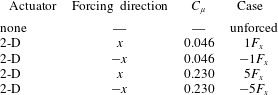
8.1 Model and flow cases
The suggested model is based on the addition of the actuator body force as a source term in the stationary, incompressible laminar boundary layer equations for the case of spanwise invariant flow (2.5-D flow) presented in appendix A. Therefore, the analysis will focus on the generalised case of spanwise-uniform forcing. The inclusion of the plasma effect can be conveniently modelled as a volume distributed body force that can be extracted with numerical or experimental means (Kotsonis Reference Kotsonis2015). It must be noted that certain assumptions are necessarily attached to such an approach. It is assumed that the external flow does not affect the plasma actuator body force (Pereira, Ragni & Kotsonis Reference Pereira, Ragni and Kotsonis2014; Dörr & Kloker Reference Dörr and Kloker2015b
, Reference Dörr and Kloker2016), and thermal effects due to plasma are weak enough to assume incompressible conditions (Kotsonis Reference Kotsonis2015). Additionally, the force is assumed to be time invariant (recall the definition of steady effect given in the previous paragraph) and of negligible magnitude in the wall-normal direction (
 $F_{y}\approx 0$
). The latter is a common assumption (Dörr & Kloker Reference Dörr and Kloker2015a
) and is essential in the boundary layer formulation of the Navier–Stokes equations as wall-normal pressure invariance (
 $\unicode[STIX]{x2202}p/\unicode[STIX]{x2202}y=0$
), upon which the system of equations (A 1)–(A 3) is based, will otherwise not hold (Schlichting & Gersten Reference Schlichting and Gersten2000). Finally,
 $x$
diffusion terms are also neglected. The stated set of assumptions allows the modification of only the
 $x$
-momentum equation as shown in (8.1),
 $$\begin{eqnarray}u\frac{\unicode[STIX]{x2202}u}{\unicode[STIX]{x2202}x}+v\frac{\unicode[STIX]{x2202}u}{\unicode[STIX]{x2202}y}=-\frac{1}{\unicode[STIX]{x1D71A}}\frac{\unicode[STIX]{x2202}p}{\unicode[STIX]{x2202}x}+\unicode[STIX]{x1D708}\frac{\unicode[STIX]{x2202}^{2}u}{\unicode[STIX]{x2202}y^{2}}+\frac{F_{x}}{\unicode[STIX]{x1D71A}}.\end{eqnarray}$$
The boundary layer equations (A 1), (8.1), (A 3) with the boundary conditions described in appendix A are integrated with the same numerical solver used for the stability analyses of § 3. The body-force field (
 $F_{x}$
), measured in the dedicated experiment of § 5, was smoothed and interpolated at the actuator’s chordwise position on the solver grid.
To investigate the effects of both forcing direction and magnitude, five cases are presently considered. Additional to the unforced baseline case, two cases consider the use of the body-force field (
 $C_{\unicode[STIX]{x1D707}}=0.046$
) of figure 7(b) oriented along and against the boundary layer flow in
 $x$
respectively, thus respecting the semi-infinite (spanwise invariant) swept wing assumption. Finally, two cases consider a fivefold body force (
 $C_{\unicode[STIX]{x1D707}}=0.230$
) oriented again along and against the flow in
 $x$
. An overview of the modelled cases, and respective notation, is given in table 3.
8.2 Results
The boundary layer solutions for the unforced,
 $5F_{x}$
and
 $-5F_{x}$
cases, at three different chordwise stations close to the actuator, are shown in figure 26. The onefold body-force results (cases
 $1F_{x}$
and
 $-1F_{x}$
) are not shown for ease of visualisation. The velocity profiles in the proximity of the actuator are inspected in the inviscid streamline system (figure 3
b) as the CFI modes directly descend from the amplitude of the cross-flow component (
 $-w_{ISL}$
).
Considering that, at the actuators location, the inviscid streamline angle is
 $-59.73^{\circ }$
from
 $x$
, forcing along
 $x$
has an enhancing effect on both the streamwise and cross-flow velocity components. The opposite holds when the induced jet is along
 $-x$
, i.e. the actuator opposes both components as shown in figure 26. However, already at
 $x/c=0.1$
, the forced flow profiles tend to collapse on the unforced flow curve, with differences of less than 2 % (figure 26
b). Considering the weak induced velocity, the body-force magnitude and spatial extent (note that the fivefold amplification affects only the body-force magnitude and not its shape) measured in § 5.2, it is expected that the actuation effects do not extend for long portions of the chord.
(a) Velocity profiles along (
 $u_{ISL}$
: dashed line) and orthogonal (
 $w_{ISL}$
: solid line) to the inviscid streamline at three different stations (upper left corner): unforced (black line);
 $5F_{x}$
(thin (blue) line);
 $-5F_{x}$
(thick (red) line). (b) Velocity difference profiles (
 $u_{ISL}^{\ast }$
: dashed line;
 $w_{ISL}^{\ast }$
: solid line) between the forced (
 $5F_{x}$
: thin (blue) line;
 $-5F_{x}$
: thick (red) line) and unforced case at same stations of (a). The wall normal axis is non-dimensionalised with the boundary layer thickness based on
 $0.99\cdot u_{ISL}$
from the local unforced profile.

The flow stability of the considered five cases is analysed with LST. The analysis presented here is limited to the stationary modes and to the unsteady modes with
 $f=200$
Hz as this frequency features high energy at the measurement location (figure 19
b). The related N factor curves are presented in figure 27. The integral effect of the forcing direction can be inspected from these plots. For all the modes, the forcing along
 $x$
has destabilising effects. Alternatively, forcing along
 $-x$
stabilises both stationary and travelling modes. The N factors for the
 $1F_{x}$
(
 $-1F_{x}$
) case lie in between the
 $5F_{x}$
(
 $-5F_{x}$
) case and the unforced flow and are not shown. These results are in agreement with the outcomes of Dörr & Kloker (Reference Dörr and Kloker2015b
, Reference Dörr and Kloker2017) and are a direct consequence of the mean-flow modifications shown in figure 26.
N factors of different modes for
 $f=0$
Hz (a) and
 $f=200$
Hz (b) (○:
 $\unicode[STIX]{x1D706}_{z}=4.5$
mm; ▫:
 $\unicode[STIX]{x1D706}_{z}=9$
mm; ♢:
 $\unicode[STIX]{x1D706}_{z}=13.5$
mm; ▵:
 $\unicode[STIX]{x1D706}_{z}=18$
mm;
 $+$
:
 $\unicode[STIX]{x1D706}_{z}=22.5$
mm): unforced (solid black line);
 $5F_{x}$
(dashed (blue) line);
 $-5F_{x}$
(dashed-dotted (red) line).

The N factor curves (figure 27) show how a rather weak and confined perturbation of the mean flow influences the flow stability characteristics, considering the integral nature of the N factors. Moreover, they show that increasing
 $\unicode[STIX]{x1D706}_{z}$
, thus driving
 $\unicode[STIX]{x1D6FD}_{r}$
and
 $\unicode[STIX]{x1D6F9}$
(
 $\unicode[STIX]{x1D6F9}=\tan ^{-1}(\unicode[STIX]{x1D6FD}_{r}/\unicode[STIX]{x1D6FC}_{r})$
) closer to zero, the CFI modes become less amplified and the forcing effect reduces. Eventually, very close to the actuator, the effect of the forcing direction inverts for waves with smaller
 $\unicode[STIX]{x1D6F9}$
i.e. waves travelling mainly along
 $x$
(not shown). However, these waves are highly stable for most of the considered flow (given the strong favourable pressure gradient) and are far from the most amplified mode thus usually they are not observed in three-dimensional boundary layers (Wassermann & Kloker Reference Wassermann and Kloker2003). The analysis presented in § 7.2.3 identified waves mainly advected along the local flow direction (roughly coinciding with
 $X$
at the measurement location). From these considerations, it is concluded here that the observed enhanced low frequency fluctuations at the measurement location must be caused by the actuator unsteady effect attributed to a combination of low frequency fluctuations directly introduced by the actuator or to nonlinear interactions between the plasma jets and local boundary layer modes. A further detailed receptivity measurement/analysis of this effect is deemed necessary to fully elucidate this effect (see also the comments of Dörr et al. (Reference Dörr, Kloker and Hanifi2017) on this point).
Summarising, it becomes evident that the
 $-x$
forcing actuator has the beneficial effect of reducing the cross-flow velocity component (figure 26) thus stabilising the boundary layer with respect to stationary and travelling CFI modes (figure 27). As shown by Dörr & Kloker (Reference Dörr and Kloker2017), the forcing direction is more effective for boundary layer stabilisation when against the mean cross-flow (i.e. along
 $z_{ISL}$
). However, the direction along which the actuators have the highest UFD authority is against the local flow (i.e. along
 $-x_{ISL}$
) as it maximises the flow blockage. Therefore, a compromise between the actuator’s UFD authority and CF counteraction can lead to the decision of aligning the actuator-induced jets with
 $-x$
, thus orienting the forcing components along
 $z_{ISL}$
and
 $-x_{ISL}$
(as shown in figure 3
b). Furthermore, the combined effect of two- and three-dimensional forcing, the former along
 $z_{ISL}$
and the latter along
 $-x_{ISL}$
, could sum together to some extent the two beneficial approaches (UFD and CF counteraction) for further stabilisation effects, in an analogous manner to the ‘formative suction’ control studied by Messing & Kloker (Reference Messing and Kloker2010).
9 Discussion and concluding remarks
An experimental investigation on the effect of AC-DBD plasma actuators on cross-flow instability (CFI) modes is performed. The flow control philosophy holds on the DRE/UFD sub-critical forcing approach, where stationary modes at smaller wavelength than the naturally dominating mode are forced with leading edge devices (Saric et al. Reference Saric, Carrillo and Reibert1998; Malik et al. Reference Malik, Li, Choudhari and Chang1999; Wassermann & Kloker Reference Wassermann and Kloker2002). Plasma actuators could potentially provide a viable alternative to passive roughness elements due to several inherent features. Firstly, their operation is easily adjustable through remote manipulation of the electric driving signal, allowing real time adaptations of forcing amplitude and frequency (Corke et al. Reference Corke, Enloe and Wilkinson2010). Additionally, through strategic fabrication and integration on the wing, varying spanwise wavelengths can be forced by activating or deactivating a selected number of actuators. Indeed, based on novel fabrication techniques, customised and low thickness actuators can be designed specifically for cross-flow instability control. The combination of these features makes these actuators ideal for active flow control throughout the entire flight envelope (i.e. for different Reynolds numbers and wing incidences). Finally, a control strategy that holds on tuning the natural flow stability, as the UFD concept, requires only moderate input energy, assuring significant net improvement in efficiency of the control device (Dörr & Kloker Reference Dörr and Kloker2017).
Despite these advantages, the use of AC-DBD plasma actuators for controlling CFI poses significant technical and theoretical challenges. Apart from reliability considerations, which pertain more to industrial applications, their inherent unsteady forcing effect becomes highly important for flight Reynolds number flows. At these regimes, primary and secondary cross-flow instabilities appear at frequencies which are of the same order as the frequencies typically used for the plasma AC high voltage (
 $O$
(kHz)). This allows for the actuator to trigger the primary travelling CF waves or secondary cross-flow instabilities and potentially promote transition, restricting any benefits from the steady UFD effect. This possibility was already highlighted by Dörr & Kloker (Reference Dörr and Kloker2017) in their numerical simulations using plasma actuators as UFD devices. However, this effect has received limited attention up to now as the published numerical studies of Dörr & Kloker (Reference Dörr and Kloker2015b
, Reference Dörr and Kloker2017), Shahriari (Reference Shahriari2016) and Dörr et al. (Reference Dörr, Kloker and Hanifi2017) consider steady (or very high frequency unsteady) body-force models for the used plasma actuators. In their experimental study, Schuele et al. (Reference Schuele, Corke and Matlis2013), which employed UFD plasma actuators on a supersonic yawed cone experiment, did not infer the unsteady flow field. This aspect is considered crucial, as CFI-dominated boundary layers are highly receptive to fluctuations (Deyhle & Bippes Reference Deyhle and Bippes1996). Therefore, the main object of the current study was the analysis of the steady as well as unsteady mechanisms pertaining to the use of AC-DBD plasma actuators as UFD devices.
Novel actuators were therefore developed, characterised and used on a
 $2.17\times 10^{6}$
Reynolds number swept wing flow. Four geometries were tested allowing one to force the critical mode, a shorter-wavelength mode and a longer-wavelength mode (i.e. a sub-critical and a super-critical mode, respectively). To isolate the wavelength effect and to better analyse the consequences of using AC-DBD plasma actuators on the unsteady flow field, a spanwise-uniform actuator was tested as well. All the actuators were operated at an AC frequency ten times higher than the most unstable travelling CFI mode. A case where the actuators were operated in the unstable CFI band was also tested for comparison. Finally, a reduced-voltage test allowed inspection of the effect on the boundary layer of lowering the forcing amplitude and to compare the actuators with passive roughness elements from a previous experiment (Serpieri & Kotsonis Reference Serpieri and Kotsonis2016).
Infrared thermography visualisation highlighted the authority of spanwise-modulated plasma actuators in conditioning stationary CFI modes at the selected wavelengths. Quantitative boundary layer measurements were carried out using high-speed PIV. These measurements corroborated the outcomes of the flow visualisation, further indicating a reduced growth for the sub-critically forced CFI, compared to the growth of the critical modes. Consequently, also the unsteady flow field (i.e. primary and secondary instability modes) showed reduced amplitudes for the sub-critical flow case in line with the DRE/UFD studies (Saric et al. Reference Saric, Carrillo and Reibert1998; Wassermann & Kloker Reference Wassermann and Kloker2002; Lohse et al. Reference Lohse, Barth and Nitsche2016). However, spectral analysis of the unsteady velocity field showed strong enhancement of fluctuations in the actuated flow cases, irrespective of the forced wavelength. The developing flow structures were further investigated and characterised through proper orthogonal decomposition and reduced-order model reconstruction analyses.
The origin of these fluctuations was traced back to two possible, concurrent mechanisms. The first mechanism relies on the direct introduction of disturbances by the unsteady body-force component of the employed actuators (referred to as unsteady effect). In the investigated conditions, LST predictions indicated no amplified primary travelling waves near the forcing frequency of 2000 Hz. However, in the forced cases, enhanced velocity fluctuations within a band significantly lower than the forcing frequency were detected, suggesting the enhancement of these instabilities through direct introduction of low frequency fluctuations (also observed in the actuator characterisation experiments) or nonlinear interactions between the actuator pulsed jets and the boundary layer modes. The second mechanism is a steady effect: the steady forcing component locally modifies the mean boundary layer, and by consequence its stability and receptivity characteristics to different modes (Dörr & Kloker, private communication). As such, the boundary layer could amplify unsteady modes, originating from the unsteady effect of the actuators or from receptivity to free stream disturbances (Dörr et al. Reference Dörr, Kloker and Hanifi2017).
This hypothesis was inspected through a simplified model, making use of numerical solutions of the forced boundary layer and linear stability theory. The outcomes of this investigation, as well as the unsteady effect, require further dedicated efforts. However, through the presented model, it was possible to show that the steady effect, at least within the coverage of linear stability, has negligible consequences on the time-invariant flow stability. No conclusions on the effects on the boundary layer receptivity can be made at this point. Furthermore, through the actuator characterisation experiment, low frequency fluctuations were observed thus suggesting the unsteady effect as the cause of the enhanced low frequency fluctuations. As a consequence of these findings, UFD plasma actuators for effective LFC need to be designed, built and operated so as to minimise the introduction of low frequency disturbances.
Additional to UFD configurations, plasma actuators can also be used to directly change the base flow to a more stable state. Forcing against the local cross-flow (along
 $z_{ISL}$
, see figure 3
b) leads to the optimum boundary layer stabilisation of CFI as it minimises the cross-flow velocity component (Dörr & Kloker Reference Dörr and Kloker2015b
). However, when the plasma forcing is against the local flow velocity (along
 $-x_{ISL}$
), the strongest effects in inducing the monochromatic forced mode are obtained. This choice is optimal for plasma-based UFD, as it maximises the local flow blockage.
Acknowledgements
This project is funded by the Netherlands Organisation for Scientific Research NWO-STW under the Veni grant. The authors are thankful to Dr M. Kloker and P. Dörr (Institut für Aerodynamik und Gasdynamik, TU Stuttgart) for fruitful discussions. The authors acknowledge the anonymous referees for their constructive comments.
Appendix A. Laminar boundary layer solution
In this appendix, the mathematical formulation and the solver details of the laminar boundary layer solutions used in §§ 3 and 8 are introduced. The 2.5-D, steady, incompressible boundary layer equations are presented in (A 1) (A 2) and (A 3) (Schlichting & Gersten Reference Schlichting and Gersten2000),
 $$\begin{eqnarray}\displaystyle & \displaystyle \frac{\unicode[STIX]{x2202}u}{\unicode[STIX]{x2202}x}+\frac{\unicode[STIX]{x2202}v}{\unicode[STIX]{x2202}y}=0 & \displaystyle\end{eqnarray}$$
 $$\begin{eqnarray}\displaystyle & \displaystyle u\frac{\unicode[STIX]{x2202}u}{\unicode[STIX]{x2202}x}+v\frac{\unicode[STIX]{x2202}u}{\unicode[STIX]{x2202}y}=-\frac{1}{\unicode[STIX]{x1D71A}}\frac{\unicode[STIX]{x2202}p}{\unicode[STIX]{x2202}x}+\unicode[STIX]{x1D708}\frac{\unicode[STIX]{x2202}^{2}u}{\unicode[STIX]{x2202}y^{2}} & \displaystyle\end{eqnarray}$$
 $$\begin{eqnarray}\displaystyle & \displaystyle u\frac{\unicode[STIX]{x2202}w}{\unicode[STIX]{x2202}x}+v\frac{\unicode[STIX]{x2202}w}{\unicode[STIX]{x2202}y}=\unicode[STIX]{x1D708}\frac{\unicode[STIX]{x2202}^{2}w}{\unicode[STIX]{x2202}y^{2}}, & \displaystyle\end{eqnarray}$$
where
 $\unicode[STIX]{x1D708}$
is the kinematic viscosity. Note that, based on flow invariance along
 $z$
, the
 $z$
-momentum equation is decoupled from the others. This set of equations is solved on a Cartesian grid (wing curvature not accounted) stretched so as to have
 $x$
coinciding with the wing curvilinear abscissa. Besides the no-slip, non-penetration conditions at the wall, Dirichlet boundary conditions are prescribed at the inflow of the domain (just after the stagnation point) with an analytical Falkner–Skan–Cooke solution at equivalent pressure gradient. At the top domain the external velocity distributions specified in (A 4) are used,
 $$\begin{eqnarray}u|_{y=\infty }=\sqrt{\boldsymbol{V}(x)^{2}-w_{\infty }^{2}};\quad w|_{y=\infty }=w_{\infty }=U_{\infty }\cdot \sin (\unicode[STIX]{x1D6EC});\quad v|_{y=\infty }=0,\end{eqnarray}$$
where
 $\boldsymbol{V}$
is the velocity vector. This quantity is retrieved from the first-order linearisation of the pressure coefficient (
 $C_{p}$
) following equation (A 5),
 $$\begin{eqnarray}|\boldsymbol{V}(x)|\approx U_{\infty }\sqrt{1-C_{p}(x)},\end{eqnarray}$$
where the vertical bars denote the vector’s magnitude. The measured pressure distribution of figure 1(a) is averaged between the two rows of pressure taps and is used in (A 5).
 $C_{p}$
is based on the free stream dynamic pressure.
The differential equations are discretised with second-order finite differences in
 $x$
and with spectral elements (Chebyshev collocation method, with 500 polynomials) along
 $y$
. The computed boundary layer was validated against Falkner–Skan–Cooke solutions and compared to hot-wire measurements (Serpieri & Kotsonis Reference Serpieri and Kotsonis2016).