1. Introduction
The goal of Informative path planning (IPP) is to find the optimal path that maximizes the information subject to budget constraints. Various applications in robotics include sensor placement for indoor temperature measurements and precipitation prediction [Reference Krause, Guestrin, Gupta and Kleinberg1], search and rescue for multi-robot [Reference Singh, Krause and Kaiser2], locomotion for quadruple robots [Reference Chang and Tseng3], and terrain monitoring for unmanned aerial vehicles (UAVs) [Reference Popović, Vidal-Calleja, Hitz, Chung, Sa, Siegwart and Nieto4]. This research focuses on IPP for terrain monitoring using a UAV. The UAV-based terrain monitoring problem is to detect the targets via a UAV as soon as possible.
If the IPP has routing constraints, this problem includes two NP-hard problems.Footnote
1
First, that the agent finds the maximal information sets
 $K$
from
 $S$
sets [Reference Nemhauser, Wolsey and Fisher5] is a set-covering problem [Reference Grossman and Wool6]. Second, that the agent finds the least route from
 $K$
subgoals is a traveling salesman problem (TSP) [Reference Lin and Kernighan7].
To address these challenges, several solution strategies have been proposed, among which two representative categories are branch-and-bound methods and iterative sampling approaches. In ref. [Reference Binney and Sukhatme8], a branch-and-bound technique is applied to the IPP problem, where the large search tree is efficiently pruned using bounded parameters. Alternatively, iterative sampling approaches have been investigated in refs. [Reference Popović, Vidal-Calleja, Hitz, Sa, Siegwart and Nieto9] and [Reference Popović, Vidal-Calleja, Hitz, Chung, Sa, Siegwart and Nieto4], where UAVs are deployed to monitor terrains at multiple resolutions. Although these methods have shown practical effectiveness, they still lack theoretical performance guarantees.
To solve the routing constraint of IPP problems, the generalized cost-benefit (GCB) method [Reference Zhang and Vorobeychik10] adopts TSP approximation algorithms and proves the theoretical guarantees in the routing constraint [Reference Flood11]. Maximizing submodular functions subject to some constraints (e.g. cardinality [Reference Nemhauser, Wolsey and Fisher5], additive budget [Reference Khuller, Moss and Naor12], and routing [Reference Zhang and Vorobeychik10]) could be solved by variant greedy algorithmsFootnote 2 with theoretical guarantees [Reference Nemhauser, Wolsey and Fisher5, Reference Feige13]. To further improve GCB performance, minimum spanning trees (MSTs) are adopted as the tree structure. The GCB-MST utilizes the submodularity of the spanning trees to boost the theoretical guarantee [Reference Lin and Tseng14]. However, the MST could not be the best spanning tree.
Illustration of the proposed method. (a) Subgoals. The red cubes and decimal numbers represent subgoals and the index of subgoals, respectively. (b) The cost-benefit spanning tree. The green points, red lines, and decimal numbers represent nodes in spanning tree, edges in spanning tree, and the index of subgoals, respectively. (c) Planning. The green points and red lines represent the path nodes and path edges, respectively.

To explore the spanning tree for UAV-based terrain monitoring problems, this research proposes cost-benefit spanning tree (CBST) algorithm, which generates subgoals as a cost-benefit objective. The parameter of CBST is able to generate the tree between the MST and the shortest path tree (SPT). To illustrate the CBST concept, as Figure 1 (a) shows, there is a UAV in the map. There are
 $6$
nodes, including
 $1$
source node (index
 $1$
). As Figure 1 (b) shows, the CBST generates the tree from six nodes. As Figure 1 (c) shows, the UAV plans the path to maximize the environmental coverage along the tree.
The contributions of this research are as follows: First, this is the first work to explore CBST for IPP problems. The proposed algorithm, CBST, is able to generate trees between the MST and the SPT. Second, this research further proves the performance bounds of spanning trees under different total curvatures. Third, the simulations and experiments demonstrate that the proposed approach outperforms the benchmark (e.g., Covariance Matrix Adaptation Evolution Strategy (CMA-ES) [Reference Popović, Vidal-Calleja, Hitz, Chung, Sa, Siegwart and Nieto4] and GCB [Reference Zhang and Vorobeychik10]).
The paper is organized as follows. Section 2 reviews the relevant work. Section 3 describes the background knowledge of this research. Section 4 introduces the problem formulation. Section 5 describes the proposed algorithms. Section 6 describes the experiments. Section 7 discusses the key issues of the proposed methods. Finally, Section 8 reports the conclusions and future work.
2. Related work
To clarify the key terms in this paper, the differences between path planning (PP), IPP, and coverage path planning (CPP) are as follows: The PP is to plan a path from location A to B [Reference Choset, Lynch, Hutchinson, Kantor, Burgard, Kavraki and Thrun15]. The IPP is to plan a path, which maximizes the information subject to a constraint [Reference Binney and Sukhatme8]. The CPP is to plan a path to completely cover a designated workspace [Reference Galceran and Carreras16]. This research focuses on IPP.
The prior works of probabilistic search, IPP, submodular maximization problems, and the Prim-Dijkstra algorithm are discussed in this section.
2.1. Probabilistic search
Probabilistic search consists of perception and decision-making [Reference Stone18]. Perception is to estimate where the target is, while decision-making is to find the optimal path. In the perception part, Bayesian filter enables agents to estimate the probability distribution of the targets [Reference Bourgault, Furukawa and Durrant-Whyte19]. However, in the decision-making part, finding the optimal solution for this problem is NP-hard [Reference Trummel and Weisinger20].
There are two steps in the perception of probabilistic search. First, a probabilistic search is used to construct a probabilistic map including the initial information. The probabilistic map is composed of cells. Each cell represents whether the target is located or not. Second, the agent runs the Bayesian filter to update the probabilistic cell of the target existing or not [Reference Chung and Burdick21, Reference Chung and Burdick22].
Occupancy grid maps updated by Bayesian filter are the most commonly used for spatial sensing in perception [Reference Elfes23]. In refs. [Reference Chung and Burdick22] and [Reference Tseng and Mettler24], the researchers show searching for one target with different parameters using a Bayesian filter. In ref. [Reference Popović, Vidal-Calleja, Hitz, Chung, Sa, Siegwart and Nieto4], the researchers show the UAV is able to execute terrain monitoring in discrete environments using Bayesian search.
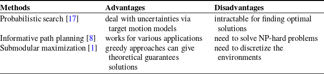
The advantage of probabilistic search is that the probabilistic model is adopted to deal with uncertainty of target motion. The disadvantage of probabilistic search is that finding the optimal actions along all possible paths is infeasible (see Table I) due to its exponentially exploded branches.
2.2. Informative path planning (IPP)
IPP is to find the optimal path for an agent to maximize the pre-defined information subject to budget constraints [Reference Lau, Huang and Dissanayake25]. The IPP problems can be classified by (i) non-adaptive and (ii) adaptive planning strategies. If the agent has information about the environment in advance, and plans the path before taking off, it is called non-adaptive method [Reference Besada-Portas, de la Torre, de la Cruz and de Andrés-Toro26], e.g., coverage methods [Reference Galceran and Carreras16, Reference Torres, Pelta, Verdegay and Torres27], Pareto optimization methods [Reference Qian, Shi, Yu and Tang28], and evolution algorithm methods [Reference Bian, Feng, Qian and Yu29]. On the other hand, if the agent is allowed to change its path online, it is called adaptive methods [Reference Nikolos, Valavanis, Tsourveloudis and Kostaras30], e.g., continuous-space informative path planner method [Reference Hitz, Galceran, ve Garneau, Pomerleau and Siegwart31], adaptive submodularity with hypothesis pruning methods [Reference Javdani, Klingensmith, Bagnell, Pollard and Srinivasa32], hybrid planner [Reference Yu, Zheng and Xu33], and non-myopic methods [Reference Singh, Krause and Kaiser2].
The IPP problem can be considered a data gathering mission involving sequential decision-making under uncertainty. This problem can be modeled as a Partially Observable Markov Decision Process (POMDP) [21], which is NP-hard. Although it is an NP-hard problem, the greedy approach can obtain near-optimal solutions [Reference Nemhauser, Wolsey and Fisher5].
In refs. [Reference Popović, Vidal-Calleja, Hitz, Chung, Sa, Siegwart and Nieto4] and [Reference Popovic, Hitz, Nieto, Sa, Siegwart and Galceran34], two-steps approach is adopted to adaptive plan strategies. First, the agents find the solutions greedily to maximize the reduction of Shannon’s entropy in the map. It is similar to frontier-based approaches for map exploration problems [Reference Yamauchi35]. Second, the agents optimize the subgoals by CMA-ES [Reference Popović, Vidal-Calleja, Hitz, Sa, Siegwart and Nieto9, Reference Popovic, Hitz, Nieto, Sa, Siegwart and Galceran34]. CMA-ES is an evolutionary approach with generic global optimization [Reference Hansen36]. Although the methods in refs. [Reference Popović, Vidal-Calleja, Hitz, Chung, Sa, Siegwart and Nieto4] and [Reference Popovic, Hitz, Nieto, Sa, Siegwart and Galceran34] are adaptive, there are no theoretical guarantees. In ref. [Reference Cui, Li and Yan37], the researchers show that multiple autonomous underwater vehicles (AUVs) are able to collect environment data efficiently by maximizing the mutual information between the scalar field model and observations. In ref. [Reference Wang, Cheng, Chi, Yan and Meng38], the researchers consider the semantic information of the focused environment to obtain the probability distribution of the target locations. Hence, it is called semantic-aware IPP.
Due to the popularity of large language model (LLM), semantic-aware IPP is proposed for object search. The semantic information is utilized for the target distribution to improve the IPP performance [Reference Wang, Cheng, Chi, Yan and Meng38]. In ref. [Reference Vashisth, Rückin, Magistri, Stachniss and Popovi’c39], semantic information is applied to segment the target with adaptive IPP. In ref. [Reference Zhang, Tian, Shao, Zhang and Liu40], without targets’ layout and locations, the mobile robot is able to investigate spatial location relations between object and room type. The research shows that the potential applications combining LLM and IPP.
The advantage of IPP is that the general formulation can solve various problems (e.g., environmental inspection, search problems). Even if probabilistic search is a special case of IPP. The disadvantage of IPP is that most of IPP are NP-hard problems, which are infeasible to find optimal solutions (see Table I). Hence, how to solve IPP with theoretical guarantees is important.
2.3. Submodular maximization problems
To solve IPP problems with theoretical guarantees, submodularity is the key. A set function is submodular if it follows the diminishing returns property. If the function is nondecreasing and submodular, greedy policies find the solutions with theoretical guarantees [Reference Nemhauser, Wolsey and Fisher5]. Various applications include map exploration [Reference Corah and Michael41, Reference Lu and Tseng42], collecting lake information [Reference Singh, Krause and Kaiser2], locating a non-adversarial target [Reference Tseng and Mettler24, Reference Hollinger and Singh43], and placing sensors for indoor temperature prediction [Reference Krause, Guestrin, Gupta and Kleinberg1].
Comparisons of search methods.

Although the submodularity of objective function is utilized, the routing constraint is still an NP-hard problem. In ref. [Reference Zhang and Vorobeychik10], the researchers propose GCB algorithm for submodular maximization problems with routing constraints. It is proved that the GCB algorithm has
 $\frac {1}{2}(1-\frac {1}{e})\widetilde {OPT}$
theoretical guarantees where
 $\widetilde {OPT} \le OPT$
. In ref. [Reference Lin and Tseng14], the researchers reformulate the routing problem as a MST to improve the guarantees to
 $\frac {1}{2}(1-\frac {1}{e})\overline {OPT}$
. This approach is based on the submodularity of routing cost trees [Reference Flood11] and recovering set functions in the Fourier domain [Reference Tseng and Mettler24, Reference Stobbe and Krause44], where
 $\widetilde {OPT} \le \overline {OPT} \le OPT$
.
The advantage of submodular maximization problems is that the objective function with submodularity can be solved by greedy algorithms with theoretical guarantees. The disadvantage of submodular maximization is that the environment needs to be discretized as sets (see Table I). If the constraint is an NP-hard problem (e.g., routing problems), the theoretical guarantees of submodular maximization problems are degraded. To improve this issue, the submodular tree approaches need to be further explored.
2.4. Multi-agent planning
Due to the high maneuverability of UAVs, multi-agent planning is also a key technology. To cover the whole area of interest, the agent tries to minimize the maximum time cost of UAVs via linear programing formulations [Reference Chen, Zhang, Wu, You and Ning45]. Simulations show that this method outperforms other methods in tasks.
To achieve missions with learning methods, multi-agent reinforcement learning approach is proposed to cooperatively control UAVs via extrinsic and intrinsic rewards [Reference Chen, Wang, Zhang, Lu, Shu and Hu46]. This approach is similar to multi-agent deep deterministic policy gradient. Compared to manual rewards, the reward function consists of three parts: encoder, forward, and reward prediction error modules. The simulations demonstrate the effectiveness of this approach.
2.5. Prim-Dijkstra algorithm
In ref. [Reference Lin and Tseng14], the MST is adopted to reformulate routing problems. However, different tree structures can lead to different solution qualities. The Prim algorithm is typically used to construct MSTs, whereas the Dijkstra algorithm is designed to compute SPTs. In ref. [Reference Alpert, Hu, Huang and Kahng47], the authors combine the Prim and Dijkstra constructions (referred to as PD) to balance two competing objectives: path length (PL) and total tree weight (TW). Here, PL denotes the distance from the source vertex to a given vertex along the current tree, while TW refers to the total weight of the entire tree. Later, in ref. [Reference Alpert, Chow, Han, Kahng, Li, Liu and Venkatesh48], the PD-II algorithm is introduced, which incorporates the total detour cost and the degree of suboptimality in PL for each node to further enhance the original PD method.
The different tree structures could generate different solutions and guarantees of IPP. This research will explore their theoretical guarantees.
3. Background knowledge
The section contains submodularity, the lower bound of GCB under the tree-structured graph, PD algorithm, and extended probability of detection (EPD).
3.1. Submodularity
The definition and illustration of submodularity are as follows:
Definition 1 (Submodularity [Reference Nemhauser, Wolsey and Fisher5]). Given a finite set
 $S=\{1,2,\ldots ,N\},$
a submodular function is a set function
 $f \, : \, 2^N \rightarrow \mathbb{R}$
that satisfies the diminishing return property. For every
 $S_A, S_B \subseteq S$
with
 $S_A \subseteq S_B$
and every
 $s \in S\setminus S_B,$
 \begin{equation} \begin{aligned} f(S_A\cup s)-f(S_A) \geq f(S_B\cup s)-f(S_B) \end{aligned} \end{equation}
holds.
To illustrate the concept of submodularity, an example is shown in Figure 2. There are three ground sets (
 $S = \{1, 2, 3\}$
).
 $S_A=\{1\}$
and
 $S_B=\{1, 2\}$
represent the selected two sets, respectively. The set
 $S_B=\{1, 2\}$
means that the sensors are selected at location
 $\unicode{x2460}$
and
 $\unicode{x2461}$
.
 $f(S_A)$
and
 $f(S_B)$
mean the coverage of sensor at location
 $\unicode{x2460}$
and
 $\unicode{x2460}$
 $\unicode{x2461}$
(see Figure 2(a, b)), respectively. The submodular gain of
 $S_A$
and
 $S_B$
after adding a set
 $s = \{3\}$
is represented by the green dashing lines (see Figure 2(c)). It is clear that the coverage function satisfies the diminishing return property Eq. (1). Alternatively, the objective function of maximizing coverage is submodular. Greedy approaches can generate near-optimal solutions even if maximal coverage is NP-hard problem.
Illustration of submodularity. The decimal number represents the selected sensor. The colorful and white areas represent the covered and uncovered areas, respectively. (a)
 $f(S_A)$
represents the covered area by
 $S_A,$
where
 $S_A = \{1\}.$
(b)
 $f(S_B)$
represents the covered area by
 $S_B,$
where
 $S_B = \{1, 2\}.$
(c) The green dash lines represent the submodular gain after adding
 $s,$
where
 $s = \{3\}.$
Left figure shows the
 $f(S_A\cup s) - F(S_A)$
and right figure shows that
 $f(S_B\cup s) - f(S_B).$
.

3.2. Lower bound of GCB
To further apply submodularity to routing constraints, some definitions and the lower bound of GCB are introduced as follows:
Definition 2 (Total curvature [Reference Conforti and Cornuéjols49]). Given a finite set
 $S = \{1,2,\ldots ,N\},$
a monotone submodular function
 $f$
, the total curvature of
 $f$
is defined as:
 \begin{equation} \kappa _f = 1 - \min _{s\in S:f(\{ s \}) \gt 0}\frac {f(S)-f(S \setminus \{ s \})}{f(\{ s \})}. \end{equation}
If the
 $\kappa _f = 0$
, then
 $f$
is modular.
Definition 3 (The largest size of feasible solution
 $K_c$
[Reference Zhang and Vorobeychik10]). Given a ground set
 $S$
and cost function
 $c$
,
 $K_c$
is defined as:
 \begin{equation} K_c = \max _{X\subseteq S}\{|X|\; | c(X) \le B\}, \end{equation}
where
 $B$
is budget,
 $c$
is the cost function.
Theorem 3.1 (Lower bound of GCB under the tree-structured graph [Reference Lin and Tseng14]). Given a submodular monotone set function
 $f$
and a tree-structured graph cost function
 $c$
, the GCB approach is to maximize f subject to the budget
 $B$
. The performance of a set X achieves
 \begin{equation} f(X)\ge \frac {1}{2}\left(1-\frac {1}{e}\right)f(\overline {X}), \end{equation}
where
 \begin{equation} \overline {X} = \arg \max _X\left\{ \, f(X) | c(X)\le B\left(1-\kappa _c + \frac {\kappa _c}{K_c}\right) \right\}. \end{equation}
3.3. Prim and Dijkstra (PD) algorithm
MST is a spanning tree of a weighted undirected graph that minimizes the total weight (TW). Prim’s algorithm is a classical greedy method for constructing an MST. In contrast, Dijkstra’s algorithm is designed to compute the shortest path from a source node to all other nodes in a weighted graph, and is commonly used to generate a SPT. To integrate the properties of both PD, the following objective function is introduced:
Definition 4 (The objective function of PD algorithm [Reference Alpert, Hu, Huang and Kahng47]). The
 $v_i$
and
 $v_j$
of PD algorithm are chosen to minimize
 \begin{equation} \begin{aligned} (\alpha \cdot l_i)+d_{ij} \; s.t. \; v_j\in T, v_i \in V - T, \end{aligned} \end{equation}
where
 $\alpha \in [0, 1]$
is a tuning parameter,
 $l_i$
is the length from source (start point) to node
 $v_i$
,
 $d_{ij}$
is the distance between
 $v_i$
and
 $v_j$
,
 $V$
is all vertices in graph, and
 $T$
is current growing tree.
Prim-Dijkstra (PD) algorithm [Reference Alpert, Hu, Huang and Kahng47] can generate different types of spanning trees. If
 $\alpha = 0$
, PD algorithm is Prim algorithm; if
 $\alpha = 1$
, PD algorithm is Dijkstra algorithm. As Figure 3(a) shows, there are six subgoals on this map. As Figure 3(b) shows, the Prim algorithm generates the MST. As Figure 3(c) shows, the Dijkstra algorithm on this map generates the SPT. In the PD algorithm, different parameters generate different spanning trees.
Illustration of the PD algorithm. (a) The complete graph. The blue points, blue edges, and decimal numbers represent subgoals, paths, and the index of subgoals, respectively. (b) Minimum spanning tree (MST). (c) Shortest path tree (SPT). (d) The tree between MST and SPT. Tuning the
 $\alpha$
parameter generates different spanning trees.

3.4. Extended probability of detection (EPD)
Informative path planning (IPP) problems can be formulated as POMDP problems [Reference Kadane and Simon50], which are NP-hard. Hence, probability of detection model is proposed. However, the assumptions of probability of detection are not realistic, i.e., the agent only moves to neighboring cells, and the sensor has no overlapping coverage. The extended probability of detection (EPD) was proposed [Reference Tseng51] to apply to real world. The definition of EPD is as follows:
Definition 5 (Extended probability of detection (EPD) [Reference Tseng51]). The agent gets the information
 $z$
. The assumptions of EPD are as follows:
-
(i) There is no target detection (
 $z = 1$
) along the path.
-
(ii) The sensing overlapping is available.
-
(iii) The agent could move to any subgoals.

The equation of the cumulative EPD is defined as
 \begin{equation} f_p(S_g) = \sum _{i=1}^{T}P(S_{g,i})\cdot g, \end{equation}
where
 $f_p$
is the cumulative EPD along the path,
 $g$
is glimpse function and
 $P(S_{g,i})$
is the probability of covered cells at the i-th subgoal. The value of glimpse function can be calculated from the confusion table.
As Figure 4 shows, the UAV’s sensing area is not fitting in its local cell. Due to the availability of sensing overlap, the probability of sensing area is recomputed. The assumption is that the UAV moves along the path without any detections (
 $z=0$
). Finally, the UAV can navigate to any subgoals instead of neighborhood areas.
Illustration of EPD assumption.

Illustration of terrain monitoring. The red cubes and decimal numbers represent subgoals and indexes, respectively. The green and black regions represent lower probability and higher probability, respectively.

4. Problem formulation
The terrain monitoring problem is defined as follows [Reference Popović, Vidal-Calleja, Hitz, Sa, Siegwart and Nieto9]: As Figure 5 shows, there are
 $6$
subgoals in a 3D map. The UAV can visit subgoals sequentially to inspect the static objects on the terrain. The detection area of higher subgoals (e.g., location 6) is larger, while that of lower subgoals (e.g., location 2) is smaller. However, the detection rate of higher subgoals (e.g., location 6) is lower due to the image quality. The goal is to maximize gain in some information-theoretic measure within a time or path budget.
The terrain monitoring problem can be reformulated as an IPP problem as follows: Given the ground set
 $S$
, and
 $|S| = N$
, the goal is to find subgoals that maximize the probability of detection subject to the routing constraints.
 \begin{equation} \max f(X) \\ s.t. \quad c(X) \le B, \end{equation}
where
 $X \subseteq S$
,
 $f$
is cumulative probability of detection function
 $f:2^N \rightarrow \mathbb{R}^{+}$
,
 $c$
is the routing cost function
 $c: 2^N \rightarrow \mathbb{R}^{+},$
and
 $B$
is the budget. The environment is known, hence
 $f$
and
 $c$
are oracles that output probability and routing cost values, respectively.
The assumptions of the problem formulation are as follows: First, the ground set of subgoal
 $(S)$
and the budget limit
 $(B)$
are given. Second, the cumulative probability of detection function
 $(f)$
and the routing cost function
 $(c)$
can be computed via the map and sensor information. Third, the theoretical guarantees only in the discrete subgoal level. Therefore, the motion control level is not considered (e.g., UAV dynamics).
4.1. Cost-benefit spanning tree (CBST)
This problem can be reformulated as a submodular maximization problem. It can achieve theoretical guarantees via GCB approaches. If the routing route is tree structure, the theoretical guarantees will be tighter than GCB [Reference Lin and Tseng14]. However, how to find an efficient spanning tree structure is a key issue.
Regardless of the distance between the information-rich vertex and the source node, the agent will always navigate to this vertex when using the GCB algorithm with a traditional shortest-path-tree (SPT)–based cost function, which can be inefficient for search tasks. Conversely, when the GCB algorithm is applied with an MST-based cost function, the agent may skip this information-rich vertex if it is located far from the source. To overcome this limitation, CBST further incorporates the benefit term
 $f$
into the cost design.
The concept of CBST is similar to that Prim-Dijkstra algorithm. The major difference is that the objective function of CBST is cost-benefit. The objective function of CBST is
 \begin{equation} \max \left(\frac {f(v_j|T)}{\alpha \cdot l_i+d_{ij}}\right),\quad s.t.\quad v_i \in T, v_j \in V - T, \end{equation}
where
 $f$
is accumulated extended probability of detection function in Eq. (7),
 $f(v_j|T)$
is equivalent to
 $f_p(S_g)$
,
 $p$
is implicit.
 $f(v_j|T)$
represents the agent go through
 $v_j$
with
 $T$
tree (path). The other notations are the same as Eq. (6) [Reference Alpert, Hu, Huang and Kahng47].
Example of MST and CBST. The vertex 1 is the source. The map is as same as Figure 3 (a). (a) Map and subgoals. The blue points, blue edges, function, and decimal numbers represent subgoals, paths, probability of each nodes, and the index of subgoals, respectively. (b) Tree structure via MST. (c) Tree structure via CBST. (d) Glimpse function (
 $g$
).

To illustrate the MST and CBST, an example is shown in Figures 5 and 6. There are
 $6$
nodes, including a source node (index
 $1$
), in the map. As Figure 5 shows, the black area has less probability than green area after agent went to
 $v_2$
and scanned the area. The scanning areas of
 $v_6$
overlaps that of
 $v_2$
,
 $v_3$
,
 $v_4$
, and
 $v_5$
since the altitude of
 $v_6$
is higher than that of
 $v_2$
,
 $v_3$
,
 $v_4$
, and
 $v_5$
. The probability of each vertex is
 $p(v_2)=0.25, p(v_3)=0.25, p(v_4)=0.25, p(v_5)=0.25$
and
 $p(v_6)=1.$
Notice that the total probability is over 1 because there is overlapping.
The tree structure of Figure 5 is shown in Figure 6.
 $v_6$
is far from
 $v_1$
in MST structure (see Figure 6(b)). On the contrary,
 $v_6$
is nearby
 $v_1$
in Figure 6(c) in CBST structure. Under such situations, GCB-CBST performs better than GCB-MST.
On the other hand, the UAV height affects the detection rate due to the image quality. As Figure 6(d) shows that the glimpse function (
 $g$
) is to describe the relationship between the UAV height and detection rate. The
 $f$
in Eq. (9) is calculated by
 $p(v_i)$
, path and glimpse function (
 $g$
), where
 $i \in \{1,\ldots ,N\}.$
4.2. Algorithm
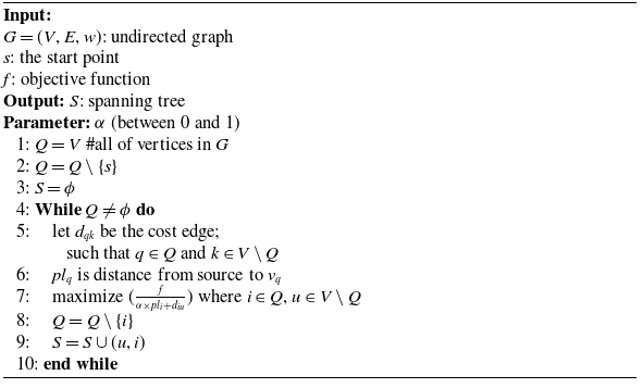
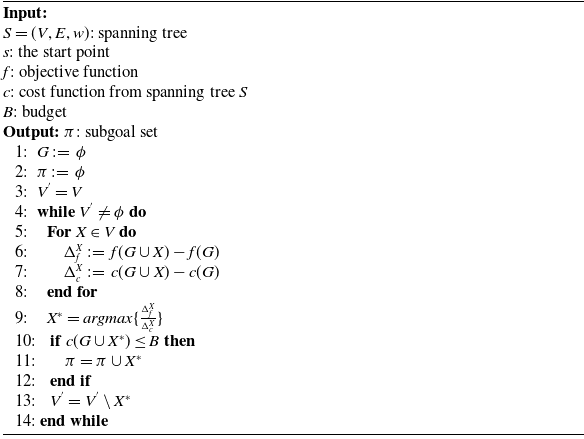
There are two algorithms: CBST algorithm and terrain monitoring algorithm. The Algorithm 1 is to generate the CBST (e.g., from Figure 1 (a) to (b)). The Algorithm 2 is to generate the path using GCB algorithm (e.g., from Figure 1 (b) to (c)).
In Algorithm 1, the inputs are an undirected graph (
 $G$
), the source (
 $s$
). The output is the spanning tree. Line
 $1$
is to build
 $Q$
(vertices in
 $G$
). Lines
 $2-3$
are initializations. Line
 $5$
is to find the distance connecting
 $v_q$
and
 $v_k$
, where
 $v_q$
belongs to the current growing tree (
 $S$
), and
 $v_k$
does not belong to the current growing tree. Line
 $6$
is to find the path length from the source vertex to
 $v_q$
along the current growing tree (
 $S$
). Line
 $7$
is to maximize
 $f/c$
, where
 $c$
is the cost function about Prim’s algorithm and Dijkstra algorithm. Lines
 $8-9$
are to update current tree and spanning tree.
Cost-benefit spanning tree

Terrain monitoring using CBST

The inputs of Algorithm 2 are
 $S$
,
 $s$
,
 $f$
,
 $c$
, and
 $B$
.
 $S$
,
 $s$
represent spanning tree from Algorithm 1 and the start point, respectively.
 $f$
,
 $c$
represent the cumulative probability of detection and cost function from spanning tree
 $S$
, respectively.
 $B$
represents the cost budget, respectively. The output
 $\pi$
represents the subgoal set with budget constraint. Lines
 $1-3$
are initializations. Lines
 $4-9$
are to find maximum cost-benefit point in the spanning tree. Lines
 $10-12$
are to select the subgoal satisfying the budget constraint. Line
 $13$
is to avoid that the agent select the subgoal repeatedly.
The primary computational steps involve iterating over vertices and edges in the spanning tree
 $S$
, with each major step taking
 $O(|V|)$
or
 $O(|E|)$
. The while loop in Line
 $4$
iterates at most
 $|V|-1$
times, and the maximizing function in line
 $7$
finds at most
 $|E|$
times. Therefore, the overall time complexity of Algorithm 1 is
 $O(|V||E|)$
. Similarly, the time complexity of Algorithm 2 is
 $O(|V||E|)$
.
5. Theoretical bound of CBST
Since the CBST could generate different spanning trees according to
 $\alpha$
parameter in Algorithm1, this section proves the theoretical guarantees of different spanning trees, SPT and MST.
To introduce the theoretical bound of CBST, the proof flow is as follows: As Figure 7 shows, the goal is to prove the theoretical guarantees of SPT and MST.
 $\kappa _c$
is the key parameter of the theoretical guarantees function and
 $\kappa _c$
is relevant to the height of SPT and MST (Theorem 5.2). Hence, Theorems 5.3 and 5.4 prove
 $\kappa _c$
of SPT and MST are 0 and 1, respectively. Then,
 $\kappa _c$
is substituted into the Theorem 3.1 to derive the theoretical bound of SPT and MST (Theorem 5.5). Theorem5.6 shows that the
 $\alpha$
in Algorithm 2 decides the tree structures (e.g., MST or SPT) and their theoretical bounds.
Illustration of the proof flow.

Theorem 5.1 (
 $\kappa _c$
in tree structure [Reference Shieh and Tseng52]). Given the tree structure of the cost function
 $c$
, then
 $\kappa _c$
either equals to
 $0$
or
 $1$
.
Since the
 $\kappa _c$
in tree structure is equal to
 $1$
or
 $0$
, the subsequent theorems focus on exploring the relationship between
 $\kappa _c$
and the height of the tree
 $(H)$
.
Theorem 5.2 (The relationship between
 $\kappa _c$
and the height of trees). Given the tree structure of the cost function and the height of the tree (
 $H$
),
if
 $H=1$
,
 $\kappa _c = 0$
;
if
 $H\gt 1$
,
 $\kappa _c = 1$
.
Proof.
W.L.O.G., we assume
 $v_1$
is the source node. To analyze the
 $\kappa _c$
, two cases of the height of tree are as follows:
Case
 $1$
: (
 $H=1$
)
 $\because$
 $H=1$
.
 $v_1$
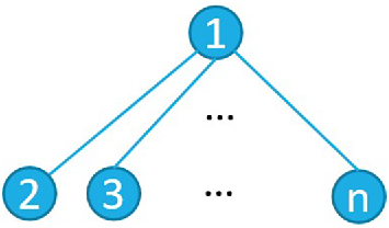
connects to the other
 $n-1$
nodes (see Figure 8).
 $\therefore \forall v_i$
are only connecting
 $v_1$
, where
 $i\in \{2,\ldots ,n\}$
,
 $n$
is the amount of nodes.
 $\Rightarrow c(v_i) = ||v_i-v_1||, i \in \{2,\ldots ,n\}$
 $\Rightarrow \kappa _c = 0$
Eq. (2)
Case
 $2$
: (
 $H\gt 1$
)
 $\therefore \exists$
the height is equal to 2 or greater than 2.
Since the case of
 $H\gt 2$
includes the case of
 $H=2$
, only the case that the height is 2 will be proved.
W.L.O.G., assume
 $v_2$
is the node of depth
 $= 1$
,
 $v_3$
is the node of depth
 $= 2,$
and the node between
 $v_1$
and
 $v_3$
is
 $v_2$
.
Let
 $S=\{v_1, v_2, v_3\}$
, and
 $s = \{v_2 \}$
 $\because c(S) = 2*(||v_1-v_2||+||v_3-v_2||)$
and
 $\begin{aligned}[t] c(S\setminus \{s\}) &= 2*||v_1-v_3|| \\ &= 2*(||v_1-v_2||+||v_3-v_2||) \\ \end{aligned}$
The first equation is by definition, and the second one is by the tree structure.
There is only one path between
 $v_1$
and
 $v_3.$
 $\therefore c(S\setminus \{s\}) = c(S)$
By definition of
 $\kappa _c$
Eq. (2),
 $\min _{s\in S:f(\{ s \}) \gt 0}\frac {f(S)-f(S\setminus \{ s\})}{f(\{s\})} = 0$
 $\therefore \kappa _c = 1$
Illustration of tree height of Theorem 5.3.

The following proofs focus on the height of SPT and MST. If height of SPT and MST is
 $H\gt 1$
or
 $H= 1$
,
 $\kappa _c$
of SPT and MST are proved.
Theorem 5.3 (
 $\kappa _c$
in SPT). Given an empty map and the SPT structure of the cost function
 $c$
, then
 $\kappa _c = 0$
.
Proof.
Given a complete graph
 $G=(V, E), V=\{ v_1,\ldots ,v_n \}$
 $\because \forall i \ne j \ne k\in \{1,\ldots ,n\}, ||v_k-v_i||+||v_i-v_j||\ge ||v_k-v_j||$
the equality only holds in the
 $v_i,v_j,$
and
 $v_k$
in a straight line.
 $\therefore$
The height of shortest spanning tree is
 $1$
, i.e. the number of maximal edges between the source node and the others is
 $1$
.
 $\because$
the height of shortest spanning tree is
 $1$
.
 $\therefore$
by Theorem 5.2,
 $\kappa _c = 0$
As Figure 8 shows, the vertex
 $1$
is the source node, and the others will be in level
 $2$
due to triangle inequality.
Since the height of MST could depend on the number of subgoals, the kissing number problem is applied for the proof. The kissing number problem investigates the maximum number of non-overlapping spheres that can touch a central sphere in a given space. It aims to determine the highest possible number of points on the surface of a sphere that can be equidistant from a fixed central point.
Theorem 5.4 (
 $\kappa _c$
in MST). Given an empty map and the MST structure of the cost function
 $c$
, the
 $\kappa _c = 1$
when
 \begin{align} (i) |n| \gt 7\; in\; 2D\; environments; \\[-30pt] \nonumber \end{align}
 \begin{align} (ii) |n| \gt 10\; in\; 3D\; environments. \\[8pt] \nonumber \end{align}
Proof.
Given complete graph
 $G=(V, E), V=\{ v_1,\ldots ,v_n \}$
W.L.O.G., we assume
 $v_1$
is the source node.
2D and 3D cases are discussed (see Figures 9 and 10).
Case (i): 2D environments
Proof by contradiction is as follows.
 $|S| \le 7$
in 2D environment.
The subgoals are arranged in the pattern of vertices of a hexagon, and the source node is in the center of a hexagon (see Figure 11).
 \begin{equation} \therefore \forall j,k \in \{1,\ldots ,n\}, ||v_1-v_j||\le ||v_j-v_k||. \end{equation}
By Eq. (12) and the property of MST, the height of MST is equal to 1.
 $\Rightarrow \kappa _c = 0.$
(by Theorem 5.2)
Hence,
 $|S| \gt 7.$
Case (ii): 3D environments
This problem can be seen as
 $\max (N)$
s.t.
 $ ||v_1-v_j||\ge ||v_j-v_k||, j,k\in \{ 1,\ldots ,N \}$
. When
 $n \gt N$
, it represents
 $H \gt 1$
 $\Rightarrow \kappa _c = 1$
Illustration of overlapping balls in Theorem 5.4. The black points, the decimal numbers, the blue lines, and the green line(s) represent the subgoals, the indexes of subgoals, the distance between source node (
 $r_1$
) and the other nodes (
 $r_2, r_3$
), and the distance between the other nodes (
 $r_2$
and
 $r_3$
), respectively. (a) The non-overlapping case. (b) The overlapping case.

Illustration of kissing balls of Theorem 5.4.

It is similar to the kissing number problem.
 $k(d)$
denotes the highest number of non-overlapping spheres in
 $\mathbb{R}^d$
that can touch another sphere of the same size.
 $k(3)=12$
has been proved [Reference Schütte and van der Waerden53], which means the maximal kissing number is
 $12$
in 3D space. The relationship between the kissing balls and the tree is as follows: As shown in Figures 9 and 10, the central sphere (
 $r_1$
) represents the root of the tree. The highest possible number of points on the surface of a sphere (
 $r_1,\ldots ,r_N$
) corresponds to the number of points (
 $N$
) (see Figure 9(a)). The overlapping spheres correspond to the distances between these points (green lines) that are smaller than the distances between these points and root (blue lines) (see Figure 9(b)).
The source node is placed on the surface (
 $x=y=z=0$
), and the other nodes are placed above the surface (
 $x \in \mathbb{R}, y\in \mathbb{R}$
and
 $z \ge 0$
). First, there are at most six points in xy plane (see Figure 10(a)). Second, since
 $k(3)=12$
, the kissing number in the upper xy plane and in lower xy plane are
 $3$
and
 $3$
, respectively (see Figure 10(b)). It represents
 $v_2,\ldots ,v_7$
are points in xy plane, and
 $v_8, v_9, v_{10}$
are upper xy plane.
 $\because$
There are no overlapping spheres.
 $\Rightarrow ||v_1-v_j||\le ||v_j-v_k||, \forall j \ne k \in \{2,\ldots ,10\}$
Finally, there are six balls in xy plane and three balls above xy plane.
 $\Rightarrow$
there are
 $9$
balls satisfying conditions.
 $\Rightarrow$
the height of MST is greater than
 $1$
if the number of subgoals greater than
 $10$
(including root) in a three-dimension environment.
 $\Rightarrow$
 $\kappa _c = 1.$
Illustration of minimum numbers of Theorem 5.4.

To give examples of the proofs, 2D and 3D cases are as follows: As Figure 11(a) shows, the source node is at the intersection point between two solid lines. If the edges of graph are
 $7$
and the subgoals are the vertices of regular heptagon, the solid blue line is greater than the dashed line. It implies that if
 $|S| \gt 7$
,
 $H\gt 1$
for MST; if the number of graph edges is
 $6$
and the subgoals are in the vertices of hexagon, the solid blue line is less than or equal to the dashed line in Figure 11(b). It implies that if
 $|S| = 7$
,
 $H=1$
for MST.
Note that if
 $|S|\le 10$
in 3D environment (see Figure 10(c)), either
 $\kappa _c = 0$
or
 $\kappa _c = 1$
is possible. As Figure 6 shows, there are
 $6$
nodes in graph. The height of MST in Figure 6 is
 $4$
, i.e.,
 $\kappa _c = 1$
.
As Figure 10(a) shows, there are at most six non-overlapping balls in xy plane. By
 $k(3) = 12$
[Reference Schütte and van der Waerden53], there are three centers upper xy-plane (see Figure 10(b)). There are at most
 $10$
points (including central point) satisfying
 $||v_1-v_j||\le ||v_j-v_k||, \forall j \ne k \in \{2,\ldots ,10\}$
.
Theorem 5.5 (The theoretical guarantees of GCB-SPT and GCB-MST). By Theorems
5.3
and
5.4
, given a submodular monotone set function
 $f,$
a MST cost function
 $c_{MST}$
with the condition of subgoals, and a SPT cost function
 $c_{SPT}$
, the GCB approach is to maximize f subject to the budget
 $B$
. The performance of a set
 $X$
with
 $c_{MST}$
and of a set
 $X$
with
 $c_{SPT}$
achieve
 \begin{equation} f(X)\ge \frac {1}{2}\left(1-\frac {1}{e}\right)f(X_{MST}), \end{equation}
and
 \begin{equation} f(X)\ge \frac {1}{2}\left(1-\frac {1}{e}\right)f(X_{SPT}), \end{equation}
where
 \begin{equation} X_{MST} = arg\max _X\left\{ f(X) | c_{MST}(X)\le B \left(\frac {1}{K_{c_{MST}}}\right) \right\}\!, \end{equation}
and
 \begin{equation} X_{SPT} = arg\max _X\{ f(X) | c_{SPT}(X)\le B \}, \end{equation}
respectively.
Proof. The MST and SPT cases are as follows:
(MST) The theoretical guarantees of GCB-MST is as follows:
By Theorem 5.4, if the subgoal condition is satisfied,
 $\kappa _{c}=1$
. Substituting
 $\kappa _{c}=1$
into Eq. (5), the budget constraint is
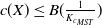 $c(X)\le B(\frac {1}{K_{c_{MST}}})$
 $\therefore X_{MST} = arg\max _X\{ f(X) | c_{MST}(X)\le B (\frac {1}{K_{c_{MST}}}) \}$
(SPT) The theoretical guarantees of GCB-SPT are as follows:
By Theorem 5.3, the
 $\kappa _{c}$
of SPT is 0. Substituting
 $\kappa _{c}=0$
into Eq. (5), the budget constraint is
 $c(X)\le B)$
 $\therefore X_{SPT} = arg\max _X\{ f(X) | c_{SPT}(X)\le B \}$
Theorem 5.6 (The theoretical guarantees of GCB-CBST). Given a submodular monotone set function
 $f$
, a CBST cost function
 $\overline {c}$
with
 $\alpha = 0$
and Eqs. (
10
) and (
11
), and a CBST cost function
 $\breve {c}$
with
 $\alpha = 1,$
the GCB approach is to maximize
 $f$
subject to the budget
 $B$
in the case of IPP on the terrain. The performances of a set X achieve
 \begin{equation} f(X)\ge \frac {1}{2}\left(1-\frac {1}{e}\right)f(\overline {X}), \end{equation}
and
 \begin{equation} f(X)\ge \frac {1}{2}\left(1-\frac {1}{e}\right)f(\breve {X}), \end{equation}
where
 \begin{equation} \overline {X} = arg\max _X\left\{ f(X) | \overline {c}(X)\le B \left(\frac {1}{K_{\overline {c}}}\right) \right\}\!. \end{equation}
and
 \begin{equation} \breve {X} = arg\max _X\{ f(X) | \breve {c}(X)\le B \}. \end{equation}
respectively.
Proof.
The numerator of the CBST objective function is fixed (see Eq. (9)). When
 $\alpha =0$
, denominator of the CBST objective function is the same as that of the MST; when
 $\alpha =1$
, denominator of the CBST objective function is the same as that of the SPT. Hence, the theoretical guarantee is the same as Eqs. (15) and (16).
Although the theoretical guarantees of CBST are the same as MST, the performance of CBST is different from that of MST due to objective function of the tree spanning. The problem is with budget constraints. The CBST spans the tree adopts cost-benefit objective, so the agent will go through the subgoal with more cost-benefit ratio than that of MST. For example, the budget is
 $3$
and the budget constraint is routing in Figure 1(a) , the path in GCB-MST is
 $\{1, 2, 3 \}$
and the path in GCB-CBST is
 $\{1,6,5 \}$
in Figure 12(a) and (b). The accumulated EPD in GCB-MST is
 $0.48$
and that in GCB-CBST is
 $0.95.$
Example of difference between GCB-MST and GCB-CBST.

6. Experiments
To evaluate the performance of different approaches, there are three experiments: the maximization extended probability of detection problem (EX1), the search problem (EX2), and Tuning
 $\alpha$
parameters (EX3). The EX
 $1$
is to evaluate the extended probability of target detection (EPD) of different offline approaches with routing constraints in simulations as Eq. (8). The EX
 $2$
is to evaluate the search time of different approaches with routing constraints in simulations and real world. The purpose of EX3 is to evaluate the influence of changing
 $\alpha$
for search results.
6.1. Experiment setup
6.1.1. Simulation setup
In the EX
 $1$
and EX
 $2$
, there are two different-sized maps. The size of map 1 and map 2 is
 $4 \times 4 \times 3$
 $(m^3)$
and
 $8 \times 8 \times 3$
 $(m^3)$
, respectively. To further evaluate the scalability, the size of map 3 is
 $100 \times 100 \times 3$
 $(m^3)$
. As shown in Figure 13, the numbers of ground set
 $|S|$
are
 $58$
,
 $58$
, and
 $714$
in maps 1, 2, and 3, respectively. The number of subgoals in low altitude is more than that in high altitude, due to the camera’s field of view (FOV). The index
 $1$
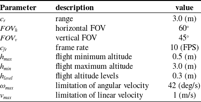
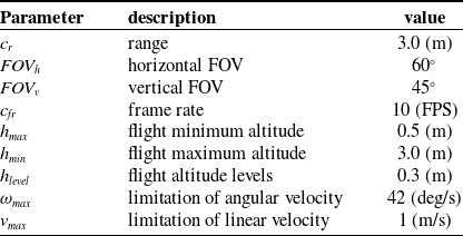
is start point. The experimental setup (e.g., camera and drone parameters) is as shown in Table II. The CPU is Intel(R) i7-8700K CPU with 3.70 GHz and 64 GB RAM.
The cost constraints are
 $10$
 $(m)$
and
 $40$
 $(m)$
, respectively. The cost function
 $c$
is measured by Euclidean distance. Note that, since computing routing cost is NP-hard problem,
 $c$
is approximated by
 $\hat {c}$
via Nearest Neighbor (NN) algorithm [Reference Rosenkrantz, Stearns and Lewis54], which provides a
 $\frac {3}{2}-$
approximation factor.
The chosen parameters in Table II are as follows: The sensing range and FOV are close to Intel Realsense cameras. The frame rate is
 $10$
Hz since the RGBD cameras work in
 $10\sim 30$
Hz. The maximal and minimum flight altitudes are based on the image quality. The higher or lower flight altitude cannot detect targets accurately. Since the fast motion leads to the images blurring, the maximal linear and angular velocities are set.
In single target scenario, the target is located in
 $121$
places uniformly. The drone searches
 $5$
times in each place. Hence, there are
 $605$
times. The search processing is as follows: The agent takes off and moves to the next subgoal. If the drone cannot find the target (
 $P(Z=1) \le 95 \%$
), the agent will go through the next subgoal until finding the target (
 $P(Z=1)\ge 95 \%$
) or utilizing all budgets.
Drone hardware setup in simulation.
Ground set in simulation.

In multiple-targets scenario, the targets are located in
 $20$
places randomly. The drone searches
 $5$
times in each place. Hence, there are
 $100$
times. The search processing is as follows: The agent takes off and moves to the next subgoal. If the drone cannot find all the targets (
 $P(Z=1) \le 95 \%$
), the agent will go through the subgoal until finding all the targets (
 $P(Z=1)\ge 95 \%$
) or utilizing all budgets.
There are two setups in the search experiments, online and offline. The online approach for the drone is to compute the information to decide the next subgoal(s); the offline approach for the drone is to compute all subgoals before taking off. There are two steps in the offline setup. First, the path is generated by algorithm subject to budget constraints offline. Second, the agent flies through the path. There are three steps in the online setup. First, the path (or the point) is generated by algorithm online. Second, the agent flies through the path. Third, the agent repeats first step via new measurements by second step until the terminal condition.
To evaluate the search performance, the expected time till positive decisions (
 $E[TTD^+]$
) is adopted [Reference Chung and Burdick22].
 $E[TTD^+]$
represents the expected time of successful searches, while
 $E[TTD]$
represents the expected time of successful and failed searches.
Along with the path, the agent updates the probability of target detection (
 $Z$
) in grid map via Bayesian filter. There are
 $20 \times 20$
and
 $40 \times 40$
grids in maps 1 and 2, respectively. When the probability of the cell in grid map is greater than
 $95\%$
(
 $P(Z = 1)\ge 95 \%$
), the agent finds the target. Once the agent finds the target, it will land, and the search time is from taking off to landing.
(a) The black points, black decimal numbers, the index 1 in black represent the subgoals, the subgoal indexes, and the source node, respectively. The blue stars and decimal numbers represent the target locations and the subgoal indexes, respectively. (b) The d435i provides the RGB images. The YOLOv5 detects the target in the image. The blue box represents the target location in the image with the detection probability.

6.1.2. Real world setup
The map in the real world is a
 $4\times 4 \times 2$
 $(m^3)$
lobby at the Mathematics Department of National Central University (see Figure 14 (a)). The target is located in 5 places randomly. The drone searches 5 times in each place. Hence, there are 125 times. The budget
 $B=10$
 $(m)$
is adopted in this map. Figure 14 (a) shows the ground set
 $|S| = 31$
and the fixed start point is the subgoal
 $1$
. The target is located in three positions (blue stars) at each search.
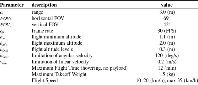
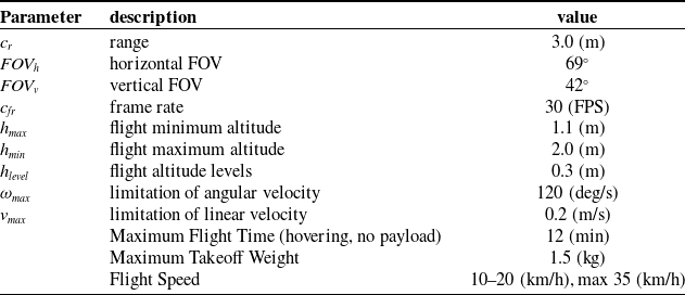
As shown in Figure 15, the TD100-EDU450 is developed by Taiwan Drone 100 corporation. Its specification is shown in Table III.
The D435i RGBD camera is used to explore the environment, while T265 camera is used to localize itself. The YOLOv5 [Reference Jocher, Chaurasia, Stoken, Borovec, Michael, TaoXie, imyhxy, Yifu, Wong, Abhiram, Montes, Wang, Fati, Nadar, Laughing and Sonck55] is adopted to detect objects running on Nvidia Jetson Xavier NX (see Figure 14(b)). The drone’s operating system is Ubuntu 18.04 and runs the Robot Operating System. The parameters of TD100-EDU450 hardware setup are shown in Table III.
Drone hardware setup and specification in real world.
The TD100-EDU450, sensors, and development board.

6.2. EX
$1$
: EPD maximization

In the experiment, the GCB-CBST is compared with four methods: A-optimality with CMA-ES [Reference Popović, Vidal-Calleja, Hitz, Chung, Sa, Siegwart and Nieto4], GCB [Reference Zhang and Vorobeychik10], GCB-MST [Reference Lin and Tseng14], and GCB-SPT. CMA-ES is online method, while the others are offline methods.
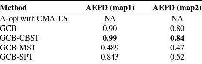
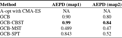
The experiment results in the Gazebo simulation are summarized in Table IV. Since CMA-ES is online algorithm, the accumulated EPD is not available. GCB-CBST outperforms other approaches in the accumulated EPD in maps 1 and 2. The tree structure of SPT is inefficient due to the repeated paths. Since the path in GCB-SPT has high cost-benefit, the accumulated EPD of GCB-SPT is higher than GCB-MST. These experiments show that GCB-CBST outperforms the other three methods in the maximal EPD problem.
EPD maximization experiment results. The accumulated extended probability of detection (AEPD) as follows.
6.3. EX
$2$
: Search experiment

The goal of the drone is to find the target as soon as possible subject to budget constraint, so the metrics in this experiment are expected time till positive decisions (
 $\mathbb{E}$
[TTD
 $^+$
]) and success rate.
In the multiple targets scenario, the metrics in this experiment are expected time till positive decisions with multiple targets (
 $\mathbb{E}$
[TTD
 $^+_m$
]) and the average number of detected objects. The E[TTD
 $^+_m$
] is defined as follows:
 \begin{equation*} E[TTD^+_m] = \frac {1}{Nn}\sum _{j=1}^{N}\sum _{i=1}^{n}t^j_i, \end{equation*}
where
 $N$
,
 $n$
, and
 $t^{\, j}_i$
represent the number of trials, number of objects in trial
 $j \in N$
, and detection time of object
 $i \in n$
in trial
 $j \in N$
. However, the search time of non-detected objects will be set to the maximal time constraint if it reaches the time constraint. The parameters are same as EX
 $1$
.
6.3.1. Simulation
In single target scenario, the expected time till positive decision (
 $\mathbb{E}$
[TTD
 $^+$
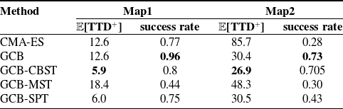
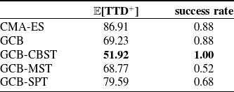
]) is compared to evaluate the search performance. GCB-CBST outperforms other four methods in
 $\mathbb{E}$
[TTD
 $^+$
]. GCB-CBST and GCB-SPT are competitive in map 1 since the drone moves to high cost-benefit subgoals. However, the success rate in GCB-SPT is less than that in GCB-CBST since the path in GCB-SPT is inefficient.
The success rates of the GCB and GCB-CBST are competitive in map 2 (see Table V). The success rate of the GCB is higher than that of the GCB-CBST in map 1 (see Table V). In the GCB-CBST path, the drone moves to the repeated subgoals. Hence, it has fewer false detections than GCB does. GCB-CBST attains a little less success rate than GCB in map1 because the drone moves to the repeated subgoals in GCB-CBST.
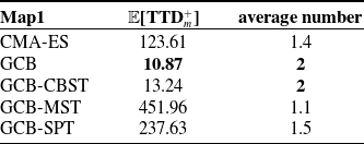
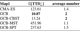
In multiple targets scenario, the average number of detected targets of the GCB and GCB-CBST is the same (see Table VII). GCB and GCB-CBST outperform the other three methods in the average number of detected targets. The E[TTD
 $^+_m$
] of the GCB and GCB-CBST is competitive (see Table VII) since the targets’ locations are random. GCB and GCB-CBST outperform the other three methods in E[TTD
 $^+_m$
].
In the single target and multiple targets scenario of large-scale simulations (map 3), the success rates and E[TTD
 $^+$
] of GCB-CBST outperform other approaches (see Table VI for single target and Table VIII for multiple targets). The computational time, CPU usage, and memory usage of GCB-CBST, GCB-MST, and GCB-SPT are very close.
Search experiment results reveal indicators success rate and
 $\mathbb{E}$
[TTD
 $^+$
] in map 1 and map 2.

Search experiment results reveal indicators success rate and
 $\mathbb{E}$
[TTD
 $^+$
] in map 3.

In summary, GCB-CBST is the best method for search tasks, since it can move through the high cost-benefit subgoals immediately and repeatedly.
Search experiment results reveal indicators the average number of detected objects and
 $\mathbb{E}$
[TTD
 $^+_m$
] in simulation.
6.3.2. Real world
The tree structures of GCB-CBST, GCB-MST, and GCB-SPT are shown in Figure 16. GCB-CBST outperforms the other four methods in
 $\mathbb{E}$
[TTD
 $^+$
] (see Table IX). The height in real world is lower than that in the simulation, so the path in GCB-SPT does not have high coverage. The
 $\mathbb{E}$
[TTD
 $^+$
] in GCB-SPT is the worst.
In single target scenario, the GCB-CBST outperforms the other four methods in success rate (see Table IX, since the GCB-CBST must go to subgoals via tree structure, and the drone moves to the repeated subgoals which have high cost-benefit values. The GCB-MST and GCB-SPT are the worst in success rate.
Search experiment results reveal indicators the average number of detected objects and
 $\mathbb{E}$
[TTD
 $^+_m$
] in map 3.

Search experiment results reveal indicators success rate and
 $\mathbb{E}$
[TTD
 $^+$
] in real world.

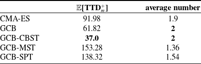
In multiple targets scenario, the GCB-CBST outperforms the other four methods in both
 $\mathbb{E}$
[TTD
 $^+_m$
] and average number (see Table X). In the GCB-MST method, the drone traverses unnecessary subgoals, resulting in the worst performance.
These experiments show that GCB-CBST outperforms the other four benchmarks in search problems.
Search experiment results reveal indicators the average number of detected objects and
 $\mathbb{E}$
[TTD
 $^+_m$
] in real world.

Three tree structures in the lobby environment. The blue circles and green circles represent the ground set and the picked subgoals, respectively. The red lines represent the paths.

6.4. EX
$3$
:
$\alpha$
tuning


The
 $\alpha$
ranges from
 $0$
to
 $1$
with an interval of
 $0.05$
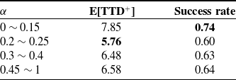
. In the map1, the alpha values generate 4 kinds of tree structures. the alpha ranges are
 $0\sim 0.15$
,
 $0.2\sim 0.25$
,
 $0.3\sim 0.4$
, and
 $0.4\sim 1$
. In the map2, the alpha values generate 6 kinds of tree structures. The alpha ranges are
 $0$
,
 $0.05$
,
 $0.1\sim 0.15$
,
 $0.2$
,
 $0.25\sim 0.5$
, and
 $0.55\sim 1$
.
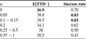
As shown in Table XI, since map 1 is not big enough, the results in different tree structures in GCB-CBST show insignificant differences. As shown in Table XII, there is significant difference between
 $\alpha =0$
and
 $\alpha =1$
since the map 2 (
 $8\times 8\times 3 (m^3)$
) is bigger than map 1 (
 $4\times 4\times 3 (m^3)$
). The cost function with parameter
 $\alpha =0$
is the best in
 $\mathbb{E}$
[TTD
 $^+$
], because the tree structure is minimum weight spanning tree. In the MST algorithm, it is possible to generate edges with the minimum total weight, which results in shorter distances between subgoals. Consequently, a better
 $\mathbb{E}$
[TTD
 $^+$
] can be achieved.
In summary, the performance when
 $\alpha$
approaches 0 is better than the performance when
 $\alpha$
approaches 1 due to the path efficiency. How to tune an optimal
 $\alpha$
is still an issue. The
 $\alpha =0$
could be a fast solution in search experiments.
Search experiment results reveal indicators success rate and
 $\mathbb{E}$
[TTD
 $^+$
] in map 1 with different
 $\alpha$
.

Search experiment results reveal indicators success rate and
 $\mathbb{E}$
[TTD
 $^+$
] in map 2 with different
 $\alpha$
.

7. Discussions
7.1. Guidance and search problems
This research focuses on the algorithms of search problems instead of guidance problems. Guidance and search problems differ in three key aspects [Reference Tseng51, Reference Chai, Tsourdos, Savvaris, Chai, Xia and Chen56]: knowledge of locations, problem formulation, and computational complexity. In guidance problems, the robot knows both the starting position (A) and the destination (B) and needs to find a path between them. In contrast, search problems involve finding an unknown target (C) without prior knowledge of its location. Additionally, guidance problems are usually continuous, meaning the robot moves through a continuous space, while search problems are often discrete, where there are distinct subgoals in the environment. Finally, when search problems are transformed into set-cover problems, they become NP-complete, making them computationally challenging to solve optimally.
The key distinction between guidance and search problems lies in the robot’s knowledge of locations. In guidance problems, the robot knows exactly where it starts (A) and where it needs to go (B), so the challenge is to determine an efficient path between the two points. In contrast, search problems involve an unknown target (C), meaning the robot must explore the environment to locate it. Since the robot does not have prior knowledge of C’s location, it must rely on strategies such as systematic scanning, probabilistic search, or heuristic exploration to find the target. This lack of information makes search problems inherently more uncertain and complex than guidance problems.
Another major difference is the problem formulation. Guidance problems are typically continuous, where the robot moves through an environment with smooth trajectories and can adjust its path dynamically. These problems are often solved using optimization techniques, control theory, or path-planning algorithms like A* or Dijkstra’s algorithm. In contrast, search problems are usually discrete, meaning the environment is covered by a set of discrete subgoals, and the robot moves step-by-step between them. The search process involves selecting the next subgoal based on prior observations, often modeled as a decision-making process in a discrete space.
Finally, guidance and search problems differ in computational complexity. While guidance problems can often be solved efficiently with deterministic algorithms, search problems become significantly harder when transformed into set-cover problems. In this formulation, the goal is to cover all possible target locations with a minimal number of sensing or search actions. This is an NP-complete problem, meaning there is no known polynomial-time algorithm to find the optimal solution. As a result, heuristic and approximation techniques, such as greedy algorithms, genetic algorithms, or probabilistic sampling methods, are commonly used to achieve near-optimal solutions within a reasonable computation time.
7.2. Potential limitations of CBST
Although CBST works well in experimental scenarios, there are some limitations of CBST. First, one of the assumptions for CBST is that the target is static. If the target is dynamic, a Bayes filter should be added to estimate the target distribution. Second, there are no obstacles between two nodes. Hence, the path cost of spanning tree is computed based on the straight line between two nodes. If there are obstacles between two nodes, path cost needs to be further estimated (e.g., receding horizon). Third, the tree structure of CBST is fixed during the search mission. If the robot tunes
 $\alpha$
online, it can expand different tree structures. However, in such cases, the theoretical guarantees are different.
8. Conclusion and future work
This research proposes the CBST tree structure to solve submodular maximization problems subject to routing constraints for terrain monitor problems. The research is summarized as follows: First, this is the first work to explore CBST for this problem. Second, to the best of our knowledge, this is the first work to prove the relationship between the theoretical guarantees and the total curvature (
 $\kappa _c$
) of tree structures. Third, the experiments show that the proposed CBST using GCB algorithm outperforms the benchmark approaches in probability of detection, search time, and success rate for both single target and multiple targets.
The future work of this research is as follows: First, the proposed CBST outperforms the benchmark in search experiments in the empty map. If there are obstacles in the map, the routing path cost needs to be further modified. Second, the GCB with tree structured graph cost function is offline approach. How to apply adaptive submodularity to tree structures is another research direction. Third, tuning alpha is going to be very map-specific. How to estimate the best alpha is a research topic. Fourth, how to apply proposed algorithms for search and rescue is an useful direction [Reference Lu, Tsai and Tseng57]. When the targets are humans, there are more uncertainties to be considered (e.g., different shapes and colors). Finally, the proposed algorithm is applied to a static target. How to extend the proposed algorithm to multiple moving targets is another potential research.
Acknowledgement
The authors would like to thank Yan-Shuo Li for his help with the simulations during the revision.
Competing interests
No conflicts of interest exist
Ethical standard
Not applicable under the heading.
Authors’ contributions
Conceptualization, Wei-Hsiang Chiu, and Kuo-Shih Tseng; methodology, Wei-Hsiang Chiu and Kuo-Shih Tseng; software, Wei-Hsiang Chiu and Kuo-Shih Tseng; validation, Wei-Hsiang Chiu and Kuo-Shih Tseng; formal analysis, Wei-Hsiang Chiu and Kuo-Shih Tseng; investigation, Wei-Hsiang Chiu and Kuo-Shih Tseng; resources, Wei-Hsiang Chiu and Kuo-Shih Tseng; data collection, Wei-Hsiang Chiu; writing–original draft preparation, Wei-Hsiang Chiu; writing–review and editing, Kuo-Shih Tseng; visualization, Wei-Hsiang Chiu; supervision, Kuo-Shih Tseng; project administration, Kuo-Shih Tseng; funding acquisition, Kuo-Shih Tseng.
Financial support
This research was completed thanks to the financial support from Taiwan NSTC 113-2221-E-008-101-MY2.
Use of AI
ChatGPT 4o is applied to revise some paragraphs of this manuscript. ChatGPT (GPT-4o, accessed October 2025) was employed to refine the manuscript’s English expression and improve readability. The tool was not used for data generation, analysis, or idea development, and all substantive content and conclusions were produced by the authors.
Supplementary material
The supplementary material for this article can be found at https://doi.org/10.1017/S0263574725102956