1 Introduction
In recent years, the world has been facing a rise in the number of extreme and in some cases catastrophic natural events. Most of these events directly influence the sea state and eventually cause complex and violent sea environments. In such cases, several mechanisms may lead to significant amplification of waves and to extreme and unexpected interaction events with marine or coastal structures, which may eventually result in human fatalities and injuries, and in structural damage or loss of structural functionality. A documentation of such extreme events can be found for example in Nikolkina & Didenkulova (Reference Nikolkina and Didenkulova2011) and O’Brien, Dudley & Dias (Reference O’Brien, Dudley and Dias2013). In light of the potential hazard posed by extreme sea waves (e.g. rogue waves), their generation mechanism is an important subject that has been extensively studied in recent decades – for reviews, see Kharif & Pelinovsky (Reference Kharif and Pelinovsky2003), Dysthe, Krogstad & Müller (Reference Dysthe, Krogstad and Müller2008) and Onorato et al. (Reference Onorato, Residori, Bortolozzo, Montina and Arecchi2013). However, the study of the interaction of extreme waves with coastal or marine structures has received less attention so far. Specifically, the mechanisms governing the wave run-up and impact on structures operating in a violent wave field are still not fully understood. Nevertheless, the identification and quantification of these aspects are essential for engineering practice. Recently, several studies have considered the developed wave run-up and impact for the case of the interaction between a complex and violent wave field and a bottom-mounted vertical cylinder (e.g. Bai & Taylor Reference Bai and Taylor2007; Li, Wang & Liu Reference Li, Wang and Liu2012, Reference Li, Wang and Liu2014; Ji et al. Reference Ji, Liu, Li and Jia2015), while, for a vertical wall, most of the research effort has been devoted to solitary wave reflection (Byatt-Smith Reference Byatt-Smith1971; Maxworthy Reference Maxworthy1976; Su & Mirie Reference Su and Mirie1980; Power & Chwang Reference Power and Chwang1984; Cooker, Weidman & Bale Reference Cooker, Weidman and Bale1997; Craig et al. Reference Craig, Guyenne, Hammack, Henderson and Sulem2006; Chambarel, Kharif & Touboul Reference Chambarel, Kharif and Touboul2009; Chen et al. Reference Chen, Kharif, Yang, Hsu, Touboul and Chambarel2015). However, using a dynamically stable (over constant bottom) and isolated wave, such as a solitary wave, limits the study of the possible mechanisms that can lead to extreme wave–wall interactions. In fact, the solitary wave–wall interaction can only address the effect of nonlinearity during wave run-up, which has also been demonstrated using the shallow-water equations (Mirchina & Pelinovsky Reference Mirchina and Pelinovsky1984; Pelinovsky, Kharif & Talipova Reference Pelinovsky, Kharif and Talipova2008). A different insight into the wave–wall interaction problem can be obtained by considering the reflection of a more general incoming wave field and taking into account the effect of dispersion. This has revealed, in the linear case, the effect of dispersion focusing on the wave run-up (Pelinovsky & Shurgalina Reference Pelinovsky and Shurgalina2010). More recently, the nonlinear and (weakly) dispersive case has been considered as well by Carbone et al. (Reference Carbone, Dutykh, Dudley and Dias2013) and Viotti, Carbone & Dias (Reference Viotti, Carbone and Dias2014), who revealed the effect of nonlinear evolution. Even for the simple case of a nearly monochromatic incident wave field, Carbone et al. (Reference Carbone, Dutykh, Dudley and Dias2013) showed how the effect of nonlinear evolution leads to a run-up of more than five times the incident wave amplitude. This remarkable outcome was found to be a result of wave amplification that occurs due to the formation of an undular bore. Further insight into the effect of undular bore formation on the wave run-up was provided by Viotti et al. (Reference Viotti, Carbone and Dias2014), who studied the conditions to obtain extreme run-up values and demonstrated a run-up of more than six times the incident wave amplitude. These results, which were found under shallow-water conditions, encourage further investigation of the influence of nonlinear evolution on the wave run-up over intermediate and deep water as well. The current study presents such an investigation, which was carried out using a numerical wave flume model. The model is based on the high-order spectral (HOS) method (Dommermuth & Yue Reference Dommermuth and Yue1987; West et al. Reference West, Brueckner, Janda, Milder and Milton1987), which preserves full dispersivity. Therefore, the model is able to simulate the evolution of nonlinear waves and their interaction with a vertical wall over a wide spectrum of water depths ranging from shallow to deep water.
The paper is organized as follows. The mathematical formulation of the problem is first constructed in § 2. The numerical approach is then detailed in § 3. In § 4, several salient phenomena that emerge due to nonlinear evolution of incident wave groups over constant water depth are identified in both shallow and deep water. The role of nonlinear wave evolution in the formation of extreme run-up events on a vertical wall are then demonstrated and analysed in § 5. Finally, conclusions are drawn in § 6.
2 Mathematical formulation
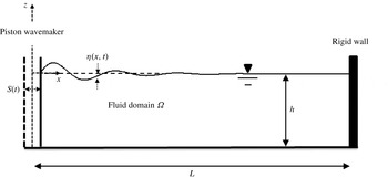
The two-dimensional wave flume considered here is illustrated in figure 1. The Cartesian coordinate system is adopted with the origin located at the intersection of the wavemaker and the mean water level. The vertical axis
 $z$
is oriented upwards and the horizontal axis
 $x$
is oriented towards the rigid wall, which is located at the end of the flume. The vertical and horizontal dimensions of the flume are denoted by
 $h$
and
 $L$
, whereas
 ${\it\eta}$
and
 $S$
represent the displacement functions of the water surface and the wavemaker, respectively. Water waves are simulated along the flume using the Euler equations, which are derived by assuming incompressible fluid and inviscid flow. These assumptions, together with the assumption of irrotational flow, successfully describe the water behaviour under fully nonlinear surface waves (Dommermuth et al.
Reference Dommermuth, Yue, Lin, Rapp, Chan and Melville1988; Bonnefoy, Le Touzé & Ferrant Reference Bonnefoy, Le Touzé and Ferrant2006).
Sketch of the numerical wave flume.

Applying the definition of a velocity potential,
 $u=\boldsymbol{{\rm\nabla}}{\it\phi}$
, the irrotational Euler system can be expressed as
 $$\begin{eqnarray}\displaystyle & {\rm\nabla}^{2}{\it\phi}=0,\quad \text{in }{\it\Omega}, & \displaystyle\end{eqnarray}$$
 $$\begin{eqnarray}\displaystyle & {\it\rho}\partial _{t}{\it\phi}+{\textstyle \frac{1}{2}}{\it\rho}(\partial _{x}{\it\phi}^{2}+\partial _{z}{\it\phi}^{2})+{\it\rho}gz+p=0,\quad \text{in }{\it\Omega}, & \displaystyle\end{eqnarray}$$
where
 $u$
is the water velocity field,
 ${\it\Omega}$
denotes the physical domain of the flume,
 ${\it\rho}$
is the water mass density,
 $g$
is the gravitational acceleration,
 $p$
is the fluid pressure and
 ${\it\phi}$
is the velocity potential. Equations (2.1) and (2.2) express the requirements for mass and momentum conservation in the flume’s domain. These requirements are subject to the following kinematical conditions on the flume boundaries:
 $$\begin{eqnarray}\displaystyle & \partial _{t}S=\partial _{x}{\it\phi},\quad \text{on }x=S(t), & \displaystyle\end{eqnarray}$$
 $$\begin{eqnarray}\displaystyle & \partial _{z}{\it\phi}=0,\quad \text{on }z=-h, & \displaystyle\end{eqnarray}$$
 $$\begin{eqnarray}\displaystyle & \partial _{x}{\it\phi}=0,\quad \text{on }x=L, & \displaystyle\end{eqnarray}$$
 $$\begin{eqnarray}\displaystyle & \partial _{t}{\it\eta}=\partial _{z}{\it\phi}-\partial _{x}{\it\phi}\partial _{x}{\it\eta},\quad \text{on }z={\it\eta}(x,t). & \displaystyle\end{eqnarray}$$
Note that (2.3) is a formulation for the special case of a piston wavemaker (as illustrated in figure 1). Neglecting water surface tension, the momentum conservation on the free water surface can be expressed through (2.2) as follows:
 $$\begin{eqnarray}\partial _{t}{\it\phi}=-{\textstyle \frac{1}{2}}(\partial _{x}{\it\phi}^{2}+\partial _{z}{\it\phi}^{2})-g{\it\eta},\quad \text{on }z={\it\eta}(x,t).\end{eqnarray}$$
In order to obtain a time-dependent solution for
 ${\it\phi}$
and
 ${\it\eta}$
, an initial condition for each of these quantities is required:
 $$\begin{eqnarray}\displaystyle & {\it\phi}(x,z,t=0)={\it\phi}^{0}(x,z), & \displaystyle\end{eqnarray}$$
 $$\begin{eqnarray}\displaystyle & {\it\eta}(x,t=0)={\it\eta}^{0}(x). & \displaystyle\end{eqnarray}$$
This completes the formulation of the mathematical model, which is implemented in this study in a non-dimensional form. The constant fluid depth
 $h$
, the water mass density
 ${\it\rho}$
and the gravitational acceleration
 $g$
are used to scale the variables. The solution of the model, which consists of the governing equations (2.1)–(2.2) together with the boundary conditions (2.3)–(2.7) and the initial conditions (2.8)–(2.9), can be obtained numerically. In this study, the non-periodic HOS method is employed. It is briefly outlined in the next section.
3 The non-periodic high-order spectral method
3.1 The potential decomposition
The HOS method provides a numerical solution for the fully nonlinear water wave problem. This method relies on the spectral collocation approach in which each of the discrete values of a considered function contributes to the evaluation of the spatial derivatives. As a result, the HOS method produces relatively high accuracy, also known as ‘spectral accuracy’ (Trefethen Reference Trefethen2000). Additionally, if the considered domain is bounded and periodic, the derivative evaluation can be efficiently implemented through the fast Fourier transform (FFT). However, in the present case, the domain is non-periodic. Such cases led to the idea of the potential decomposition concept (Agnon & Bingham Reference Agnon and Bingham1999), where the original problem is decomposed into a sum of two problems. The first problem is periodic. This problem is derived by imposing reflecting lateral boundary conditions. The second problem is called the additional problem and satisfies the movable lateral boundary conditions. Such a decomposition technique is allowable due to the linearity of the Laplace equation (2.1). Therefore, the solution of a non-periodic problem can be expressed as
 $$\begin{eqnarray}{\it\phi}={\it\phi}_{p}+{\it\phi}_{a},\end{eqnarray}$$
where the subscripts
 $p$
and
 $a$
stand for periodic and additional, respectively. This approach allows each problem to be solved separately, where the additional potential may represent a ‘steady’ flow, which can be obtained analytically out of the time stepping process. The spatial solution of the periodic potential can be represented by classical standing wave solutions. The solution in time is obtained by adding back the two potentials to satisfy the remaining boundary conditions on the free water surface, where the additional solution is used as a forcing term. In this way the accuracy and efficiency that characterize the original HOS method are preserved for non-periodic problems as well.
3.2 The solution for the additional potential
The additional solution may stand for a wavemaker condition, absorbing layer condition, elastic boundary, etc. In the present study, the additional problem should satisfy the piston wavemaker condition at the flume entrance (see figure 1). Specifically for a linear wavemaker condition, the formulation for
 ${\it\phi}_{a}$
is expressed as follows:
 $$\begin{eqnarray}\left.\begin{array}{@{}c@{}}{\rm\nabla}^{2}{\it\phi}_{a}=0,\quad \text{in }{\it\Omega},\\ \partial _{x}{\it\phi}_{a}=\partial _{t}S,\quad \text{on }x=0,\\ \partial _{z}{\it\phi}_{a}=0,\quad \text{on }z=-1,\\ \partial _{x}{\it\phi}_{a}=0,\quad \text{on }x=L.\end{array}\right\}\end{eqnarray}$$
Following Agnon & Bingham (Reference Agnon and Bingham1999), a solution for the additional potential problem defined in (3.2) can be achieved with quadratic polynomials. It is well known that the polynomial solutions for the Laplace equation in the current two-dimensional domain are found from the real and imaginary parts of
 $$\begin{eqnarray}(x+\text{i}z)^{n},\quad n=0,1,2,\ldots .\end{eqnarray}$$
Confining to
 $n\leqslant 2$
, and applying the lateral and bottom boundaries expressed in (3.2), the quadratic solution for the additional potential is obtained as
 $$\begin{eqnarray}{\it\phi}_{a}=\frac{\partial _{t}S}{2L}[(z+1)^{2}-(x-L)^{2}],\quad \text{in }{\it\Omega}.\end{eqnarray}$$
Adding back the periodic and the additional problems, the conditions at the lateral and bottom boundaries of the flume are satisfied. The remaining conditions to satisfy are the free boundary conditions.
3.3 The numerical solution of the free surface equations
The difficulties of treating the free boundary conditions are attributed to two types of nonlinearities. The first one is rather obvious and it is reflected by unknown quantities that multiply each other. The second nonlinearity is the required conditions on the unknown free surface. For the sake of the second type of nonlinearity, it is advantageous to modify the free surface boundary conditions described in (2.6) and (2.7). The objective of the modification is to formulate the conditions with dependence on the horizontal coordinate only. This is partially achieved by formulating the free surface conditions in terms of the periodic surface potential. Following Zakharov (Reference Zakharov1968), the periodic surface potential is defined as follows:
 $$\begin{eqnarray}{\it\phi}_{p}^{s}={\it\phi}_{p}(x,z={\it\eta},t).\end{eqnarray}$$
Introducing the derivatives that stem from this definition (
 $\partial _{x}{\it\phi}_{p}=\partial _{x}{\it\phi}_{p}^{s}-\partial _{z}{\it\phi}_{p}\partial _{x}{\it\eta}$
and
 $\partial _{t}{\it\phi}_{p}=\partial _{t}{\it\phi}_{p}^{s}-\partial _{z}{\it\phi}_{p}\partial _{t}{\it\eta}$
) into the free boundary conditions and using the separated potential representation, the non-dimensional free surface boundary conditions can be expressed as follows:
 $$\begin{eqnarray}\left.\begin{array}{@{}c@{}}\partial _{t}{\it\eta}=W[1+(\partial _{x}{\it\eta})^{2}]+\partial _{z}{\it\phi}_{a}-(\partial _{x}{\it\phi}_{p}^{s}+\,\partial _{x}{\it\phi}_{a})\partial _{x}{\it\eta},\\ \partial _{t}{\it\phi}_{p}^{s}={\textstyle \frac{1}{2}}W^{2}[1+(\partial _{x}{\it\eta})^{2}]-{\textstyle \frac{1}{2}}(\partial _{z}{\it\phi}_{a})^{2}-{\textstyle \frac{1}{2}}(\partial _{x}{\it\phi}_{p}^{s}+\partial _{x}{\it\phi}_{a})^{2}-\partial _{t}{\it\phi}_{a}-{\it\eta},\end{array}\right\}\quad \text{on }z={\it\eta}(x,t).\end{eqnarray}$$
Using Zakharov’s formulation leaves the modified free boundary conditions with the periodic vertical velocity
 $W=\partial _{z}{\it\phi}_{p}(x,z={\it\eta},t)$
as the only non-free surface component. Owing to its periodicity, this quantity can be evaluated following the original HOS method (Dommermuth & Yue Reference Dommermuth and Yue1987; West et al.
Reference West, Brueckner, Janda, Milder and Milton1987) as
 $$\begin{eqnarray}\left.\begin{array}{@{}c@{}}W=\displaystyle \mathop{\sum }_{m=1}^{M}W^{(m)},\\ W^{(m)}=\displaystyle \mathop{\sum }_{j=0}^{m-1}\frac{{\it\eta}^{j}}{j!}\partial _{z^{j+1}}{\it\phi}_{p}^{(m-j)}(x,0,t),\quad m=1,2,\ldots ,M,\end{array}\right\}\end{eqnarray}$$
where
 $M$
is the order of nonlinearity and
 ${\it\phi}_{p}$
can be expressed as
 $$\begin{eqnarray}\left.\begin{array}{@{}c@{}}{\it\phi}_{p}=\displaystyle \mathop{\sum }_{m=1}^{M}{\it\phi}_{p}^{(m)},\\ {\it\phi}_{p}^{(m)}=\displaystyle \mathop{\sum }_{n=0}^{N}A_{n}^{(m)}(t)\frac{\cosh [k_{n}(z+1)]}{\cosh k_{n}}\cos k_{n}x,\end{array}\right\}\end{eqnarray}$$
defined by
 $k_{n}=n{\rm\pi}/L$
, the wavenumbers, and
 $N$
, the number of wave modes that are considered. In this study, all the simulations are performed with
 $M=8$
, whereas the value of
 $N$
is selected specifically for each simulation. This completes the implementation of the non-periodic HOS method, which can be summarized with the following steps. First, decompose the problem into the periodic and the additional problems and derive the solution of the additional potential separately and according to the given lateral boundaries. Then, the two problems are added back to satisfy the free boundary conditions, where the additional derivatives
 $\partial _{z}{\it\phi}_{a}$
,
 $\partial _{x}{\it\phi}_{a}$
and
 $\partial _{t}{\it\phi}_{a}$
are calculated analytically and serve as forcing terms. Finally, the solution for
 ${\it\phi}_{p}^{s}$
and
 ${\it\eta}$
at each time step is obtained via the original HOS method, through which spatial derivatives are efficiently computed utilizing the FFT algorithm, and the time derivatives are treated by means of a numerical time stepping scheme. In the current study the classical fourth-order Runge–Kutta (RK4) scheme is used.
3.4 Initial conditions
The simulations in the current study are initiated by the motion of the piston wavemaker with the following stroke function definition:
 $$\begin{eqnarray}S(t)=S_{0}\exp \left(-\left(\frac{t-{\it\tau}}{{\it\mu}T_{0}}\right)^{2}\right)\cos ({\it\omega}_{0}(t-{\it\tau})),\quad \text{on }x=0.\end{eqnarray}$$
This generates a periodic wave modulated by a Gaussian envelope, where
 ${\it\mu}$
controls the envelope width. The highest stroke amplitude,
 $S_{0}$
, is related to the maximum wave amplitude,
 $a_{0}$
, through the wavemaker’s amplitude-to-stroke ratio denoted by
 $r_{piston}$
(see Dean & Dalrymple Reference Dean and Dalrymple1991),
 $$\begin{eqnarray}\frac{a_{0}}{S_{0}}=r_{piston},\quad r_{piston}=\frac{2(\cosh 2k_{0}-1)}{\sinh 2k_{0}+2k_{0}},\end{eqnarray}$$
where
 $k_{0}$
is the carrier wavenumber associated with
 ${\it\omega}_{0}$
through the linear dispersion relation. In addition,
 $T_{0}=2{\rm\pi}/{\it\omega}_{0}$
defines the carrier wave period and
 ${\it\tau}$
controls the initiation of the wavemaker motion. The latter is imposed in order to avoid abrupt wavemaker motion, which may result in unstable evolution.
The adopted numerical approach enables one to consider nonlinear waves while preserving full dispersivity. Therefore, extreme run-up events that emerge due to the effect of nonlinear wave evolution can be investigated over a wide range of water depths. As a first step of the investigation, the salient phenomena that arise during nonlinear evolution of unidirectional wave groups over constant water depth are identified (without wave reflection). This step is considered in the following by placing the wall far enough from the wavemaker.
4 Nonlinear evolution of incident wave groups
Nonlinear evolution of wave groups over constant water depth is accompanied by several salient phenomena. In general, these phenomena arise due to imbalance between nonlinear and dispersion effects. Considering a focused wave group in deep water, the group tends to spread and lose its height due to dispersion. However, nonlinear effects act oppositely and cause front steepening of the group. In shallow-water conditions, a similar discussion may be introduced. However, in this case, the dispersion property is weak and the nonlinear effects dominate the initial stages of wave evolution. In both deep- and shallow-water conditions, a balance state may be obtained without wave breaking by disintegration into stable wave forms in which wave amplification is detected. In the following, the disintegration phenomenon is reviewed in a simple manner, by comparing the present numerical model with reduced models in both depth conditions.
4.1 Nonlinear evolution in shallow water
A short review of the evolution characteristics is provided by comparing the results of a propagated wave group following the present model and the shallow-water equations (SWE). In this way, the review also provides verification of the present model to compute waves in shallow-water conditions. The SWE are derived assuming a hydrostatic pressure distribution (dispersion effects are neglected). Using the horizontal component of the water velocity,
 $u$
, the SWE are formulated as follows (see e.g. Stoker Reference Stoker1957):
 $$\begin{eqnarray}\displaystyle & \partial _{t}u=-u\partial _{x}u-\partial _{x}{\it\eta}, & \displaystyle\end{eqnarray}$$
 $$\begin{eqnarray}\displaystyle & \partial _{t}{\it\eta}=-\partial _{x}[u({\it\eta}+1)]. & \displaystyle\end{eqnarray}$$
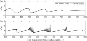
The solution of (4.1) and (4.2) is obtained through the same spectral approach for the spatial derivatives and by employing the RK4 scheme for the time stepping. Finally, the length of the flume is chosen to be sufficiently long in order to avoid wave reflection from the opposite edge. The results for the numerical examination appear in figure 2 for two evolution stages, the steepening stage (figure 2 a) and the disintegration stage (figure 2 b).
Long-term evolution in shallow water, using the SWE and the present model: (a) the steepening stage, obtained at non-dimensional time
 $t=1250$
; and (b) the disintegration stage, obtained at
 $t=2000$
. The group parameters and the numerical parameters are
 $a_{0}=0.05$
,
 $k_{0}=0.03$
,
 ${\it\mu}=2$
,
 ${\it\tau}=5T_{0}$
,
 $N=3000$
and
 ${\rm\Delta}t=0.5$
.

At the initial stage of evolution in shallow water, nonlinear effects cause crest steepening. This behaviour is clearly observed in figure 2(a) following both models. However, the agreement between the models is violated in the second stage of evolution (see figure 2 b). Following the SWE model, waves steepen until the fronts develop into a bore (see e.g. Stoker Reference Stoker1957; Madsen, Fuhrman & Schäffer Reference Madsen, Fuhrman and Schäffer2008), which usually breaks into a moving turbulent zone. Accounting for dispersion, different bore transition is observed through the present model. The wave crests evolve into a smooth undulation known as an undular bore, which finally disintegrates into a train of solitary waves ordered by height. Such a scenario occurs when the bore is weak – see Favre (Reference Favre1935), Peregrine (Reference Peregrine1966), Soares Frazao & Zech (Reference Soares Frazao and Zech2002) and Pelinovsky, Shurgalina & Rodin (Reference Pelinovsky, Shurgalina and Rodin2015) regarding the conditions for the generation of an undular bore.
As for the present analysis, the most important outcome is the wave amplification that emerges during the disintegration process. Following figure 2(b), the leading crest can reach more than twice the initial carrier wave amplitude. Such amplification values have also been demonstrated experimentally (Soares Frazao & Zech Reference Soares Frazao and Zech2002), analytically (El, Grimshaw & Smyth Reference El, Grimshaw and Smyth2006) and numerically (Soares-Frazao & Guinot Reference Soares-Frazao and Guinot2008; Tissier et al. Reference Tissier, Bonneton, Marche, Chazel and Lannes2011; Viotti et al. Reference Viotti, Carbone and Dias2014). The amplification value is strongly dependent on the initial carrier wavenumber and amplitude (Viotti et al. Reference Viotti, Carbone and Dias2014). Later in this paper, the dependence on the initial carrier wavenumber with fixed initial amplitude is further identified.
Amplification of waves due to nonlinear evolution is not confined to shallow-water conditions. Similar evolution characteristics also appear under deep-water conditions, where similar amplification emerges.
4.2 Nonlinear evolution in deep water
In deep water, dispersion effects dominate the wave group evolution. As the SWE were found to approximate the wave evolution in shallow water, the linear dispersive equations (the linear model) approximate the evolution in deep water when the nonlinear effects are weak. Therefore, here, the review for the evolution characteristics in deep-water conditions is provided through numerical examples that compare the evolution of a wave group following the present model and the linear model. The latter is solved in the same manner as outlined in § 3, but the non-dimensional free surface equations reduce to
 $$\begin{eqnarray}\partial _{t}{\it\eta}=\partial _{z}{\it\phi},\quad \partial _{t}{\it\phi}=-\,{\it\eta},\quad \text{on }z=0.\end{eqnarray}$$
In the first example, the bandwidth parameter
 ${\it\mu}$
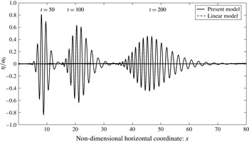
is selected to be small enough in order to generate a wide frequency range that results in significant dispersion effects. The dispersive behaviour of the wave group is indeed noticeable in figure 3.
Wave group evolution along the flume at three values of the non-dimensional time
 $t$
. The group parameters and the numerical parameters are
 $a_{0}=0.01$
,
 $k_{0}=4$
,
 ${\it\mu}=2$
,
 ${\it\tau}=5T_{0}$
,
 $N=1600$
and
 ${\rm\Delta}t=0.05$
.

The comparison of the two models in figure 3 shows a complete overlap of both solutions, following the linear and the present models. However, different group evolution may occur when nonlinear effects are more significant. This can be generated by increasing
 ${\it\mu}$
and the carrier wave steepness parameter,
 ${\it\varepsilon}_{0}=k_{0}a_{0}$
, thus reducing the dispersion effects and increasing the nonlinear effects, respectively.
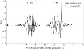
Figure 4 shows comparison results of the evolution of a wave group with higher values of
 ${\it\mu}$
and
 ${\it\varepsilon}_{0}$
. These results clearly show the deviation of the present model prediction from the prediction obtained by the linear model. The linear model shows the same evolution characteristic, where the group constantly disperses. In contrast, following the solution of the present model, the group envelope considerably steepens due to nonlinear effects. Envelope steepening is clearly observed in the first stage of evolution (
 $t=100$
), in which a ‘secondary envelope’ starts to emerge. The envelope starts to disintegrate into two envelope solitons. Analytical verification for this phenomenon was proposed by Zakharov & Shabat (Reference Zakharov and Shabat1972), which was followed by experimental verification (Yuen & Lake Reference Yuen and Lake1975; Su Reference Su1982).
The envelope disintegration process is more prominent in the second stage of evolution (
 $t=160$
). This process corresponds to a significant spectrum widening, in which substantial transfer of energy occurs from the initial narrow spectrum (determined by
 ${\it\mu}$
) to sub- and super-harmonics (Clamond et al.
Reference Clamond, Francius, Grue and Kharif2006). Such an energy transfer arises due to nonlinear resonant interactions, which occur if
 $k_{0}>1.363$
(Benjamin & Feir Reference Benjamin and Feir1967). Additionally, the disintegration process in deep water also involves significant wave amplification. Following Clamond et al. (Reference Clamond, Francius, Grue and Kharif2006), the amplified waves can reach more than twice the initial carrier wave amplitude. Significant amplification is also observed in figure 4.
In summary, nonlinear evolution of wave groups involves significant amplification in both conditions, shallow and deep water. Such wave amplifications will lead to extreme run-up events in situations where the wall is located in the area where waves are amplified. In order to identify the locations of maximum wave amplification (using the stroke function in (3.9)), and in order to link those locations and the corresponding amplification values to the water depth parameter, a numerical investigation is performed over a wide range of water depths. The results of this investigation are summarized in a diagram, which is referred to as the ‘amplification diagram’.
Wave group evolution along the flume at two values of the non-dimensional time
 $t$
. The group parameters and the numerical parameters are
 $a_{0}=0.04$
,
 $k_{0}=4.93$
,
 ${\it\mu}=3.5$
,
 ${\it\tau}=16T_{0}$
,
 $N=1600$
and
 ${\rm\Delta}t=0.05$
.

4.3 The amplification diagram of waves over a constant bottom
The amplification diagram is constructed following a set of numerical simulations which are carried out through the present model. Waves are generated following (3.9), where
 $S_{0}$
is adjusted to obtain a fixed value for
 $a_{0}$
. The numerical simulations are divided into three series. The first series describes the results versus
 $k_{0}\in [0.01,4.5]$
and with
 ${\it\mu}=2$
. In the second series, the results are given for a smaller range of the water depth parameter,
 $k_{0}\in [1.5,4.5]$
, and with
 ${\it\mu}=3.5$
. The simulations for the third series are conducted for the same range as in the second series but with
 ${\it\mu}=5$
. This division also allows the effect of the bandwidth parameter in deep-water conditions to be studied.
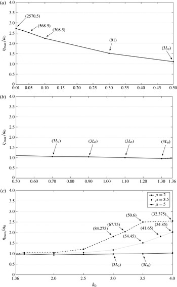
The results are summarized in the amplification diagram that is presented in figure 5. The diagram classifies three regions corresponding to different group evolutions. These are: ‘disintegration into solitary waves’, which occurs for shallow water with
 $k_{0}\leqslant 0.5$
; ‘stable and dispersive region’, corresponding to intermediate depths with
 $0.5<k_{0}<1.36$
; and ‘disintegration into envelope solitons’, which meets the condition
 $k_{0}>1.36$
of Benjamin & Feir (Reference Benjamin and Feir1967) and refers to deep water.
Plots of amplification factor versus water depth parameter for
 $a_{0}=0.05$
: (a) amplification due to disintegration into solitary waves, (b) spreading in the stable and dispersive region, and (c) amplification due to disintegration into envelope solitons. Numbers in brackets refer to the location of the detected point.

In the amplification diagram of figure 5, a few locations,
 $x_{max}$
, where the relevant amplification is detected are shown in parentheses. The minimum distance allowed equals three times the carrier wavelength (
 $3L_{0}$
), and it was chosen to avoid the amplifications that exists in the close vicinity of the wavemaker. Significant amplification appears in shallow water
 $k_{0}\leqslant 0.1$
, where the crests are disintegrated into solitary waves, and in deep water
 $k_{0}>1.36$
, where wave groups are disintegrated into envelope solitons. In between, the waves are stable and dispersive. In this region, amplification is not detected and the groups demonstrate constant spreading with different rates. Such a dispersive behaviour also dominates in deep water for lower values of
 ${\it\mu}$
, as was demonstrated previously. For higher
 ${\it\mu}$
and as
 $k_{0}$
increases, the amplification in deep water seems to increase as well, whereas the distance
 $x_{max}$
decreases. In shallow water, as
 $k_{0}$
increases, the amplification factor seems to decrease and
 $x_{max}$
decreases correspondingly.
Following the amplification diagram, wave groups that may develop extreme interaction events with a certain structure due to a nonlinear evolution effect can be identified. In the following, the amplification diagram is used to investigate and analyse situations of extreme wave run-ups that develop on a vertical wall. In particular, the following investigation aims to reveal the effect of the nonlinear wave evolution on the wave run-up in deep-water conditions, and therefore to provide an extension to similar investigations which were performed under shallow-water conditions (Carbone et al. Reference Carbone, Dutykh, Dudley and Dias2013; Viotti et al. Reference Viotti, Carbone and Dias2014). The significance of the nonlinear evolution effect is emphasized by comparing the run-up predictions of wave groups using the present model and the linear model.
5 Extreme run-up events on a vertical wall
5.1 Extreme run-up events in shallow water
In shallow-water conditions, extreme run-up events are considered for wave groups that are characterized by
 $k_{0}=0.01$
,
 $k_{0}=0.03$
and
 $k_{0}=0.05$
. Following the amplification diagram (figure 5), extreme run-ups for these groups can be generated by placing the wall at
 $x=2500$
,
 $x=850$
and
 $x=550$
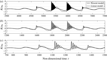
, respectively. The results for these cases of interaction are obtained for both the present model and the linear model. These results are displayed in figure 6.
Extreme run-up events on a vertical wall for three different wave groups characterized by: (a)
 $k_{0}=0.01$
, (b)
 $k_{0}=0.03$
and (c)
 $k_{0}=0.05$
. For all cases,
 $a_{0}=0.05$
,
 ${\it\mu}=2$
and
 ${\it\tau}=5T_{0}$
. The numerical parameters used in the simulations are (a)
 $N=5000$
,
 ${\rm\Delta}t=0.5$
, (b)
 $N=1700$
,
 ${\rm\Delta}t=0.5$
and (c)
 $N=1100$
,
 ${\rm\Delta}t=0.5$
.

The run-up
 $R$
is normalized by the initial carrier wave amplitude
 $a_{0}$
. The results of the present model demonstrate how the maximum run-up
 $R_{max}$
can reach approximately
 $6a_{0}$
(see figure 6
a). The maximum run-up seems to increase as
 $k_{0}$
decreases. This observation differs from that of Carbone et al. (Reference Carbone, Dutykh, Dudley and Dias2013), who stated that the maximum run-up as a function of
 $k_{0}$
takes a maximum value for
 $k_{0}\approx 0.0315$
. However, in Carbone et al. (Reference Carbone, Dutykh, Dudley and Dias2013), the investigation was performed without changing the location of the wall. Therefore, wave groups characterized by
 $k_{0}<0.0315$
could not develop a complete amplification before interacting with the wall. Recently, the investigation of Carbone et al. (Reference Carbone, Dutykh, Dudley and Dias2013) has been extended by Viotti et al. (Reference Viotti, Carbone and Dias2014), who studied the conditions for worst-case scenarios of wave–wall interaction. In particular, they concluded that the run-up potential depends on the available evolving distance (or time) prior to the interaction with the vertical wall. Following this conclusion, Viotti et al. (Reference Viotti, Carbone and Dias2014) showed how
 $R_{max}$
increases with decreasing
 $k_{0}$
and by adjusting the appropriate horizontal domain according to the location of the maximum group amplification. This outcome is in agreement with the present results.
For further comparison with the result of Viotti et al. (Reference Viotti, Carbone and Dias2014), the time-dependent run-up result of the group characterized by
 $k_{0}=0.05$
can be considered (refer to figure 6
c in the present study, and figure 7c in Viotti et al. (Reference Viotti, Carbone and Dias2014)). This comparison also shows fair agreement. However, some differences can be noticed, which arise from the use of different wave group envelopes. Finally, the notable difference between the results following the present and the linear models is considered. The run-up values following the linear model are roughly twice the incident amplitude values, which are indeed expected in these cases where dispersion hardly affects the wave transition. On the other hand, the present model shows that the run-up can be as large as
 $6a_{0}$
. This striking difference arises due to the effect of both nonlinear evolution and nonlinearity during wave run-up.
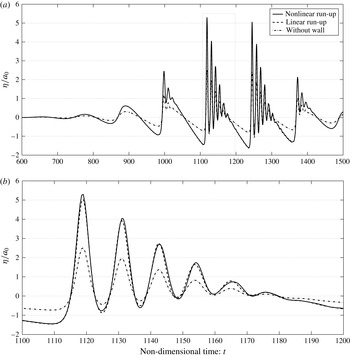
Free surface elevation at the location of the wall (
 $x=550$
) versus time: linear and nonlinear run-up of a wave group with
 $k_{0}=0.05$
. (a) Entire time interval; (b) zoom-in on the most amplified crest (the thin dotted box in panel (a)).

The latter can be evaluated separately by comparing the surface elevation at the location of the wall with and without the nonlinear terms. Such a comparison is shown in figure 7 for the wave group characterized by
 $k_{0}=0.05$
. The nonlinear run-up results (solid line) are calculated with the present model, while the linear run-up results (dashed line) are simply plotted by multiplying by 2 the results of the surface elevation without the wall in place (dashed-dotted line).
Considering the most amplified crest highlighted in the dotted box and in figure 7(b), it is observed that the effect of nonlinearity results in a small correction. This observation can be explained by examining the result of the highlighted crest without the wall in place. The highest wave that emerges in this case shows an amplification of approximately
 ${\it\eta}_{max}/a_{0}\approx 2.5$
(see also figure 5
a), which corresponds to an elevation of
 ${\it\eta}_{max}=0.125$
. In shallow-water conditions, the contribution of the nonlinear terms to the run-up for such an incident wave amplitude (or amplitude-to-depth ratio in dimensional variables) indeed results in a small correction (see e.g. Cooker et al.
Reference Cooker, Weidman and Bale1997; Chambarel et al.
Reference Chambarel, Kharif and Touboul2009). In contrast, the effect of nonlinearity of extremely high waves under shallow-water conditions may result in run-up of approximately three times the incident wave amplitude (see Chambarel et al.
Reference Chambarel, Kharif and Touboul2009).
5.2 Extreme run-up events in deep water
The investigation for extreme run-ups in deep water is classified according to the bandwidth parameter,
 ${\it\mu}$
, where three values are considered,
 ${\it\mu}=3.5$
,
 ${\it\mu}=5$
and
 ${\it\mu}=7$
. Concerning the case where
 ${\it\mu}=3.5$
, extreme run-ups are examined for two different wave groups characterized by
 $k_{0}=3.5$
and
 $k_{0}=3.8$
. The locations of the wall are selected to be close to the locations where the maximum wave amplification occurs. Therefore, following the amplification diagram (figure 5), the locations of the wall for
 $k_{0}=3.5$
and
 $k_{0}=3.8$
are chosen to be at
 $x=50$
and
 $x=40$
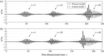
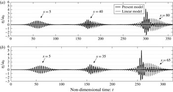
, respectively. The results for the two interaction events are given in figure 8.
Surface elevation for wave groups characterized by (a)
 $k_{0}=3.5$
,
 ${\it\tau}=9T_{0}$
and (b)
 $k_{0}=3.8$
,
 ${\it\tau}=10T_{0}$
. For both cases,
 $a_{0}=0.05$
and
 ${\it\mu}=3.5$
. The numerical parameters used in the simulations are (a)
 $N=2000$
,
 ${\rm\Delta}t=0.05$
and (b)
 $N=1600$
,
 ${\rm\Delta}t=0.05$
.

Figure 8 shows the evolution of the groups at three different stages. At these stages, the results following the present model are compared with the corresponding linear results. At the first stage of evolution, the groups are found close to the wavemaker and the results following the linear and nonlinear analyses are still in agreement. However, at the focusing stage that appears in the middle of each graph, a deviation appears between the results, due to nonlinear effects. Finally, in the third stage shown at the right side of each graph, the groups are reflected from the wall. At this stage, a notable difference is revealed between the run-up results of the present and the linear models. This is caused by the combined effect of nonlinear evolution and nonlinearity during wave run-up. The difference is also caused by the dispersive behaviour of the linear solution, which leads to a run-up that is lower than
 $2a_{0}$
. In contrast to the linear solution, the maximum run-up detected by the present model is approximately
 $4a_{0}$
.
This observation highlights the potential of extreme run-ups that exceed by far the prediction of the linear theory in deep-water conditions. Further insight into this phenomenon is gained by looking into the case where
 ${\it\mu}=5$
. Extreme run-ups in this case are generated for wave groups characterized by
 $k_{0}=3$
and
 $k_{0}=3.2$
. Following the amplification diagram (figure 5), the wall positions are chosen to be at
 $x=80$
and
 $x=65$
, respectively. The results for the group evolution and reflection are shown in figure 9. At this point, it should be noted that the selection for
 $k_{0}$
is limited. For higher values of
 $k_{0}$
, extremely large steepness values are obtained in the vicinity of the wall, which leads to a computational breakdown. The same limitation also holds for
 ${\it\mu}=3.5$
, where extreme interaction results could not be generated for
 $k_{0}>3.8$
.
Surface elevation for wave groups characterize by (a)
 $k_{0}=3.0$
and (b)
 $k_{0}=3.2$
. For both cases,
 $a_{0}=0.05$
and
 ${\it\mu}=5$
,
 ${\it\tau}=12T_{0}$
. The numerical parameters used in the simulations are (a)
 $N=3200$
,
 ${\rm\Delta}t=0.05$
and (b)
 $N=2600$
,
 ${\rm\Delta}t=0.05$
.

The results shown in figure 9 are similar to the ones observed for
 ${\it\mu}=3.5$
. The same evolution characteristics of the groups appear here as well. However, the run-up values are revealed to be higher, with a maximum run-up that exceeds
 $5a_{0}$
for the wave group defined by
 $k_{0}=3.2$
(see figure 9
b).
Larger run-up values are indeed expected in this case due to higher wave amplifications which characterize these wave groups; see the amplification diagram (figure 5). This demonstration indicates that the potential to obtain extreme run-up events is highly dependent on the bandwidth parameter in deep water.
As a final examination, a group characterized by
 ${\it\mu}=7$
and
 $k_{0}=3$
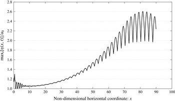
is considered. This examination aims to further emphasize the influence of the bandwidth parameter and to identify the effect of nonlinearity during wave run-up under deep-water conditions. As this case is not present in the amplification diagram, a simulation without the wall in place (placed far enough to avoid reflection) is first performed. The results that are outlined in figure 10 show the amplification development of the group during the propagation along the flume. The amplification graph is strongly oscillatory due to the fact that waves in deep water travel faster than the group envelope. The local maximum in the amplification of the group occurs when a wave crest is located at the position of the envelope peak. Then, the amplification reduces locally because the crest travels faster than the envelope. The amplification increases again as the distance between the following crest and the peak of the envelope decreases. This repeated pattern leads to the notable oscillations of the amplification graph. Further, the global evolution of the group amplification is also considered. It is characterized by an increase during the disintegration process. Then, a moderate decrease of the graph ensues when the initial envelope is significantly separated. The peak amplification factor and the corresponding spatial location are
 $$\begin{eqnarray}{\it\eta}_{max}/a_{0}=2.604\quad \text{and}\quad x_{max}=81.64.\end{eqnarray}$$
Following figure 10, many possible positions that may lead to an extreme run-up can be selected. An attempt was made to place the wall close to the maximum group amplification point (
 $x=80$
). However, the computation of this case failed due to extremely large steepness values that developed in the vicinity of the wall. Thus, the wall was chosen to be at
 $x=70$
. At this point, the amplification value is
 $$\begin{eqnarray}\max _{t}[{\it\eta}(x=70,t)]/a_{0}=2.126.\end{eqnarray}$$
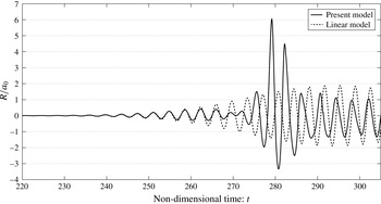
The run-up values observed in this case of interaction are presented in figure 11. Following the present model, the maximum run-up exceeds
 $6a_{0}$
. This is more than three times the run-up result of the linear model. Additionally, by comparing this result with the maximum run-up obtained for the group with the same
 $k_{0}$
but with
 ${\it\mu}=5$
, the effect of
 ${\it\mu}$
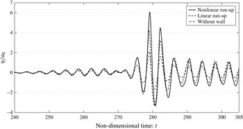
on the potential to obtain higher run-up values is demonstrated again. Finally, the effect of nonlinearity in the run-up stage is considered in figure 12. As before, this effect is presented by comparing the linear and nonlinear run-ups of the wave group at the location of the wall.
Maximum amplification factor versus location along the flume. The group and the numerical parameters are
 $a_{0}=0.05$
,
 $k_{0}=3$
,
 ${\it\mu}=7$
,
 ${\it\tau}=16T_{0}$
,
 $N=6000$
and
 ${\rm\Delta}t=0.05$
.

Extreme run-up event on a vertical wall for a wave group characterized by
 $a_{0}=0.05$
,
 $k_{0}=3$
,
 ${\it\mu}=7$
and
 ${\it\tau}=16T_{0}$
. The numerical parameters used in this simulation are
 $N=2800$
and
 ${\rm\Delta}t=0.05$
.

Comparison between linear and nonlinear run-ups of a wave group characterized by
 $a_{0}=0.05$
,
 $k_{0}=3$
,
 ${\it\mu}=7$
and
 ${\it\tau}=16T_{0}$
.

As shown in figure 12, the nonlinear terms provide a significant contribution. Unlike shallow-water conditions, for which nonlinearity depends on the maximum incident amplitude in the vicinity of the wall,
 ${\it\eta}_{max}$
, nonlinearity in deep water depends on its steepness,
 $k{\it\eta}_{max}$
. Therefore, for the current investigation, in which wave groups were initiated with a carrier wave amplitude of
 $a_{0}=0.05$
, the effect of nonlinearity during wave run-up is found to be far more significant in deep water than in shallow water (recall the results in figure 7).
6 Conclusions
In this study, the role of nonlinear wave evolution in the formation of extreme run-up events on a vertical wall has been investigated. To this end, a numerical flume model has been constructed. The model is based on the non-periodic HOS method, which provides an efficient and accurate way to simulate wave generation, propagation and reflection. In addition to computational benefits, the model is able to treat highly nonlinear waves while maintaining full dispersivity. The latter has allowed previous studies to be extended by revealing the effect of nonlinear evolution on the wave run-up under deep-water conditions.
The investigation has considered wave groups composed of a periodic wave modulated by a Gaussian envelope to represent the incoming wave field. These wave groups are easily defined using
 $k_{0}$
,
 $a_{0}$
and
 ${\it\mu}$
, which are the initial carrier wavenumber, initial carrier wave amplitude and bandwidth parameter, respectively. In the first step of the investigation, the phenomena that characterize the nonlinear evolution of the considered wave groups were identified. The most important outcome for the present investigation is the wave amplification. In shallow-water conditions (
 $k_{0}\leqslant 0.1$
), amplification occurs due to disintegration of the crests into an undular bore. In deep-water conditions (
 $k_{0}>1.36$
), the groups are amplified during a disintegration process into envelope solitons. A quantitative summary of the amplification results versus
 $k_{0}$
for a fixed value of
 $a_{0}=0.05$
is provided in the amplification diagram (figure 5). The results also show the effect of
 ${\it\mu}$
in deep-water conditions. Following the diagram, wave groups that may develop extreme interaction events with a considered structure due to nonlinear evolution effects can be identified.
In the second step of the investigation, extreme interaction events were demonstrated and analysed for the fundamental case of wave interaction with a vertical wall, in which the effect of nonlinearity in the run-up stage was considered as well. In shallow-water conditions, decreasing
 $k_{0}$
can result in higher run-up values as the amplification factor increases. In addition, for the value of
 $a_{0}$
that has been selected here, the effect of nonlinearity in the run-up stage has been found to be weak. In deep-water conditions, higher run-up values can appear by increasing
 $k_{0}$
or
 ${\it\mu}$
. This conclusion can derive directly from the amplification diagram (figure 5). However, those parameters possess an additional role which cannot be revealed from the diagram. They also control the effect of nonlinearity during wave run-up. Increasing
 $k_{0}$
or
 ${\it\mu}$
leads to higher steepness of the incident waves in the vicinity of the wall, and therefore to a greater contribution of the nonlinear terms to the wave run-up. Finally, it is noted that the most significant interaction events that have been detected reveal maximum run-up values that exceed six times the initial carrier wave amplitude. This result has been demonstrated in both shallow-water and deep-water regions.
As final remarks, it should be noted that the extreme interaction scenarios demonstrated here may be unexpected following the current design practice. This has been clearly revealed by Carbone et al. (Reference Carbone, Dutykh, Dudley and Dias2013) for the simple case of a nearly monochromatic incident wave field. As the problem of wave run-up constitutes a fundamental problem for many practical applications, the design procedure for its assessment should be further augmented and improved. To this end, the study of the mechanisms leading to extreme interaction events should be extended. It is anticipated that additional effects will emerge by considering the more general three-dimensional interaction problem, which consists of a multi-directional wave field.
Acknowledgement
This study was supported by the Israel Ministry of Science, Space and Technology, contract no. 605404541.