




No CrossRef data available.
Did New Deal Grant Programs Stimulate Local Economies? A Study of Federal Grants and Retail Sales During the Great Depression
Published online by Cambridge University Press: 15 March 2005
Abstract
Using data on New Deal grants to each U.S. county from 1933 to 1939, we estimate how relief and public works spending and payments to farmers through the Agricultural Adjustment Administration influenced retail consumption. On a per capita basis, we find that an additional dollar of public works and relief spending was associated with a 44 cent increase in 1939 retail sales. In contrast, the AAA seems to have had a negative effect on retail sales, suggesting that nonlandowners in the farm sector suffered disproportionate declines in income as a result of the AAA.
Information
- Type
- ARTICLES
- Information
- Copyright
- © 2005 The Economic History Association
The New Deal launched the most dramatic peacetime expansion of the federal government in U.S. history. The Roosevelt administration launched a myriad of new federal programs, including regulations and federal mandates, social insurance programs, and an unprecedented amount of new federal spending. Annual federal outlays outside of the traditional categories of national security and international affairs were four to six times higher in the 1930s than in 1929.1
U.S. Bureau of the Census, Historical Statistics, p. 1115, series Y471.
Popular histories often portray the New Deal as a successful antidote to the Great Depression.2
See Black, Franklin Delano Roosevelt, for example, for a favorable recent assessment of Roosevelt's efforts during the Great Depression.
Macroeconomic investigators Brown, “Fiscal Policy”; and Peppers, “Full Employment,” dismiss the New Deal as a true example of Keynesian fiscal stimulus on the grounds that the federal government did not run budget deficits of the size that a Keynesian would have deemed necessary to offset the large gap in unemployment. Bernanke and Parkinson, “Unemployment”; and DeLong and Summers, “How Does Macroeconomic Polisy,” suggest that much of the recovery in the latter half of the 1930s was the result of the natural tendency of the economy to return to its steady state. Meanwhile, Romer, “What Ended the Great Depression,” finds that the recovery after 1933 was primarily the result of monetary expansion.
Cole and Ohanian, “New Deal.”
Higgs, “Regime Uncertainty.”
See Wallis and Benjamin, “Public Relief” and “Private Employment”; Margo, “Employment”; Sundstrom, “Did the WPA”; and Fleck, “Marginal Effect.”
See Wright, “Political Economy”; Wallis, “Employment,” “Political Economy of New Deal Spending Revisited,” and “Political Economy of New Deal Spending”; Anderson and Tollison, “Congressional Influence”; Couch and Shughart, Political Economy; Fleck, “Electoral Incentives,” “Value,” “Inter-party Competition,” and “Population”; and Fishback, Kantor, and Wallis, “Can the Three R's.” Powell's recent book FDR's Folly paints a negative picture of the effectiveness of the New Deal, while citing many of these studies.
Because the New Deal involved such a wide variety of different programs, some long-lived and others short-term and experimental in nature, it is no surprise that recent research offers conflicting views of the New Deal's effectiveness. Because the New Deal targeted diverse segments of the economy, it is likely that the money spent on the different programs had quite different effects on local economies. Instead of viewing the New Deal in the aggregate, in the article we focus on the disparate impacts of the centerpieces of the New Deal's relief and recovery efforts: the federal grants that provided work relief and that led to the construction of public works; and the payments to farmers through the Agricultural Adjustment Administration (AAA). These programs accounted for 60 percent of federal New Deal spending during the period and, politically, they had the most direct impact on voters. Relief and public works spending had many broad similarities in that the grants typically were used to provide the unemployed with jobs on a range of public works projects. Even today, there are reminders of these New Deal programs in the form of public buildings, dams, roads, and other facilities that are still in operation. In contrast, the AAA grant payments were specifically designed to pay farmers to take land out of production. Thus, the net effects of AAA spending were likely to be quite different from those of relief and public works spending.
From a variety of perspectives, the New Deal offers a unique opportunity to learn how federal expenditures can influence local economies. The New Deal represented the beginning of the federal government's direct attempts to stimulate local economies, there was substantial geographic variation in how New Deal grants were distributed, and there were great differences in the pace of recovery across the country during the course of the Great Depression. To measure the economic impact of these programs, we have constructed a data set that measures federal spending on public works and relief and on agriculture in over 3,000 counties from 1933 to 1939. We then examine how the programs influenced a general measure of economic activity—retail sales. Retail sales serve as a strong proxy for personal consumption of durable and nondurable goods, which has been considered a key variable in understanding the Great Depression.8
See Temin, Did Monetary Forces; and Romer, “Great Crash.”
In the next two sections we give a sense of the variation across counties in the changes in per capita retail sales during the 1930s and in the distribution of New Deal grants. We then use this variation to estimate the relationship between the growth rate of per capita retail sales and New Deal spending, while controlling for a variety of other factors that have been found to be important in cross-sectional studies of income growth. Given that New Deal funds were likely distributed in response to the economic situation in each county, we use instrumental variables to control for potential endogeneity. The results suggest that the two major categories of New Deal grants had quite different effects on local economies. Increases in public works and relief grants contributed to significant increases in retail sales. Meanwhile, AAA grants may have aided the farmers who received them, but, by drawing farmland out of production, may have lowered the incomes of farm workers. The net effect may have been to slow the pace of economic recovery in these agricultural communities.
BRIEF OVERVIEW OF THE GEOGRAPHIC VARIATION IN THE GREAT DEPRESSION
In this article we use per capita retail sales as our proxy for local economic activity.9
Because our analysis throughout the article focuses on per capita retail sales, we will henceforth use “retail sales” and “per capita retail sales” interchangeably.
See U.S. Senate, “Expenditure,” pp. xi–xiv; and Williams, Federal Aid, p. 212. In its publicity publications, the U.S. Public Works Administration, America Builds, pp. 20–22, traced the paths of workers' spending to show the impact of the PWA on retail sales and the rest of the economy.
U.S. Bureau of Economic Analysis, GNP, p. 11.
The 1930s was a decade of lost output for the economy as a whole, but there was substantial variation in the experiences across individual counties. By 1933 both real per capita GDP and per capita retail sales had fallen to approximately two-thirds of their 1929 peaks. In per capita terms real retail sales returned to its pre-Depression level by 1939, and real GDP returned to its 1929 level by 1940.12
See series T81 deflated by series E135 and series F4 in U.S. Bureau of the Census, Historical Statistics, pp. 210–11, 224, and 843. See also Romer, “What Ended the Great Depression.”

NEW DEAL GRANTS
The crisis of the Great Depression led the Roosevelt administration to distribute unprecedented amounts of federal money in the form of nonrepayable grants. The federal government distributed $16.5 billion in nonrepayable grants over a six-year period. The grants represented a new role for the federal government during peacetime, as the New Deal increased the federal government's outlays as a share of GDP from about 4 to 8 percent. Furthermore, the federal government began spending large amounts of money where it had spent very little before, setting the stage for a long-term structural shift in the financial responsibilities of the national, state, and local governments.13
Our measure of New Deal spending does not encompass all federal spending, so our analysis does not address the impact of all forms of federal expenditures. It should be noted, however, that much of the New Deal represented an entirely new role for the federal government. For example, agricultural spending, relief spending, many forms of lending to state and local governments, and insurance of mortgage loans broke new ground for the federal government. In addition, there were major increases in federal spending from the early 1930s on roads, public buildings, public works, and conservation. The New Deal programs caused federal intergovernmental and direct outlays on education to rise from $26 million in 1932 to $235 million in 1934, on highways from $217 million to $599 million, on public welfare and employment security from $2 million to $585 million, on housing and urban renewal from $0 in 1932 to $3 million in 1934 to $71 million in 1936. Spending on the primary tasks of the federal government prior to the 1930s generally did not display the same marked jumps. See Wallis, “Why 1933?”; and U.S. Bureau of Census, Historical Statistics, pp. 1124–26.
Wallis, “Birth,” pp. 141–42.
In 1940 the U.S. Office of Government Reports (OGR) produced county-level statistics on federal spending on over 30 New Deal programs for the period 3 March 1933 through 30 July 1939.15
Much of the debate over the determinants of the state-level distribution of New Deal spending relied on information from the Office of Government Reports. Recently, scholars have expanded the debate to use the county-level information. See Fishback, Kantor, and Wallis, “Can the Three R's,” for a table that summarizes the various studies of the distribution of federal New Deal expenditures. Couch, Atkinson, and Wells, “New Deal”; and Couch and Williams, “New Deal,” have used county-level data from Alabama to examine the distribution of New Deal agricultural and total funds. Using another data source, Fleck, “Marginal Effect” and “Inter-party Competition,” has used county-level data to examine the distribution of relief and its impact on unemployment.
The U. S. Office of Government Reports, “County Reports,” also provided information on $10.4 billion in repayable loans under a variety of programs as well as data on the Federal Housing Administration's insurance of $2.7 billion in mortgage loans. We do not focus attention on these programs for several reasons. First, the nature of the loans and insurance were substantially different from the nonrepayable grants and it is hard to determine the true dollar size of the benefits that the counties received. Second, in the analysis we seek to reduce problems of endogeneity by using instrumental variables. We face difficulties in finding enough effective instruments that will allow us to simultaneously identify more than two or three New Deal variables in a system of equations. Third, by omitting the loans and FHA insurance we reduce measurement error at the risk of increasing omitted variables bias in our estimates of the impact of New Deal grants. We do not believe that the bias will be large from omitting the loans and FHA insured loans because these variables are largely orthogonal to the grants variables.
See Clarke, Roosevelt's Warrior, pp. 62–68; and Schlesinger, Age, pp. 263–96.
The federal New Deal expenditures that provided the primary aid to the farm sector came through the AAA's payments to farmers to remove land from production. The impact of the AAA grants on retail sales was likely smaller than the impact of the relief grants and potentially even negative. On the one hand, farm owners might have received higher net incomes from the AAA program. Payments typically exceeded the income farmers would have earned on the land that they took out of production because the least productive land was removed first. If the AAA succeeded in raising farm prices, the farmers also would have earned more on the crops they produced. In addition, the higher prices and the limits on land usage would have encouraged farmers to raise yields on the land they kept under cultivation. On the other hand, the AAA might well have had an adverse effect on the incomes of farm laborers, tenants, and sharecroppers. There is evidence that sharecroppers and tenants did not receive their full share of the AAA payments on the lands that they had cultivated and that some were demoted to wage laborers.18
See Whatley, “Labor”; Biles, South, pp. 39–43; and Saloutos, “New Deal.”
See Alston, “Tenure Choice.”
Table 2 shows the variation in state averages for the major grant categories, as well as summary statistics for the variation within states. As was the case with the recovery in retail sales, there was substantial variation in the extent of per capita New Deal spending across the country. The patterns of New Deal spending across states and within states differed for the two broad categories. Spending on relief and public works was over $125 per person in the heavily urbanized states in the Northeast and Midwest and was well over $200 per person in many western states. Meanwhile, relief and public works expenditures were below $80 per person in many southern states. AAA expenditures were highest in agricultural regions, particularly the West North Central region and the Mountain West. The South received substantially higher amounts per capita than did the Northeast, but much less than the amounts spent in the West and the West North Central.

SUMMARIZING THE IMPACT OF NEW DEAL GRANTS ON RETAIL SALES
Using the cross-sectional variation in retail sales growth and New Deal spending across U.S. counties, our objective in the article is to estimate an empirical growth model that produces reduced-form estimates of the impact of New Deal grants on local economic activity. Our empirical model controls for a variety of factors that would have influenced economic growth and retail expenditure patterns. The reduced-form estimate will be an amalgam of a series of interactions between New Deal grants, a variety of forms of private spending and production, income, and ultimately retail consumption.20
We summarize these effects here and provide a more formal description of the various interactions in Appendix 2 of Fishback, Horrace, and Kantor, “Did New Deal Grant Programs.” The framework we develop is based on Oates's, Fiscal Federalism, model of fiscal federalism.
Models of fiscal federalism suggest federal grants may influence local income and, hence, retail sales in a number of ways. First, regional models show that an additional dollar in grants raises local income relatively more as the share of after-tax income spent on goods and services produced within the county rises. Second, the marginal grant expenditure will have a relatively smaller effect if the spending crowds out private activity. The AAA explicitly involved a significant degree of crowding-out because it required farmers to remove land from production in a national effort to raise farm prices. The crowding-out caused by the public works and relief programs was likely to be more subtle. Given that there was such high unemployment in the 1930s, the public works and relief grants might have succeeded in providing temporary employment and relief for those who had no private opportunities. Therefore, we might expect the crowding-out effect to have been rather modest. The existing evidence offers a mixed picture, however. John Wallis and Daniel Benjamin find evidence that an additional relief job led to a one-half job reduction in the private sector.21
Wallis and Benjamin, “Private Employment.”
Margo, “Employment.”
Fleck, “Marginal Effect.”
Third, New Deal spending might have raised the productivity of local producers if it was devoted to building infrastructure that cut transport costs to other areas and thus raised the net price that local sellers received. Cuts in production costs from New Deal infrastructure potentially had either positive or negative effects on local incomes based on the extent to which the public capital enhancements either substituted for or complemented labor.24
There also remains the possibility that the improvement in private productivity from the additions to civil infrastructure had no short-term effect on private incomes, as it expanded production-possibilities without stimulating demands for the products. Recent empirical work investigating the impact of civil infrastructure on economic growth gives mixed support to the hypothesis that more infrastructure spending leads to substantial increases in economic growth. See Aschauer, “Is Public Expenditure”; Costa, Ellson, and Martin, “Public Capital”; Duffy-Deno and Eberts, “Public Infrastructure”; Hulten and Schwab, “Public Capital Formation”; Garcia-Mila and McGuire, “Contribution”; Munnell, “Infrastructure”; Gramlich, “Infrastructure”; Fernald, “Roads”; and Pereira and Flores de Frutos, “Public Capital Accumulation.”
Fourth, the impact of federal grants might have been enhanced if they stimulated additional state and local spending on projects that would not have been built otherwise. The overall impact of this response was probably small because state and local governments faced significant legal restrictions in their ability to run deficits during the 1930s, so changes in state and local government spending were likely to be matched by offsetting changes in taxes. On the other hand, to the extent that state and local governments reduced their own spending on public works as the federal government implemented fresh spending under the New Deal, the measurable impact of the federal grants would be small.25
See Gramlich, “Intergovernmental Grants”; Hines and Thaler, “Flypaper”; and Bailey and Connolly, “Flypaper,” for discussions of ways in which different types of grants influence total state and local spending. The WPA and FERA contained matching provisions in their original legislation. The FERA matching provisions were largely ignored after November 1933. The actual share of the WPA and FERA projects financed by the state and local governments varied dramatically from project to project in ways that suggest no consistent matching formula. For information on the WPA's matching provisions, see Howard, WPA, p. 147; and for the FERA see Williams, Federal Aid, p. 217.
Finally, New Deal grants may have created a fiscal drag if higher resulting incomes from the New Deal grants caused people to pay higher income taxes or encouraged them to purchase goods subject to excise taxes. Federal income and excise tax rates were uniform across the country, and the size of this effect was not likely to be large because fewer than 7 percent of households were paying income taxes during the 1930s.
Given the lack of income data at the county level during the 1930s, we develop our empirical model to estimate the impact of New Deal grants on retail sales growth instead. The ratio of retail sales to personal income at the national level was approximately 0.53, so if we were to find that an additional dollar of New Deal grants raised retail spending by 53 cents, we might conclude that income in the county rose by roughly a dollar.26
This is an estimate at the mean of retail sales. The same ratio would hold at all levels of retail sales if the elasticity of personal income with respect to retail sales is one. To get a sense of the income elasticity, we estimated it for 1929 using a cross-section of state aggregates for per capita personal incomes and retail sales. The elasticity was 0.76. Using an income elasticity of 0.76, the ratio of retail sales to personal income would range up to 0.57 when per capita retail sales are $100 above the mean to 0.50 when per capita retail sales are $100 below the mean.
DATA CONSIDERATIONS
The precision of our estimates of the impact of New Deal grants on retail sales is constrained in part by the availability of data. The Census Bureau first began collecting annual retail sales information for each county in the United States in 1929 and performed retail censuses for the years 1933, 1935, and 1939. The OGR reported data on spending in each U.S. county for the whole period between 3 March 1933 and 30 June 1939 for each of about 30 New Deal programs.27
The data set consists of 3,060 counties and county/city combinations in the United States. The New Deal program information was reported for some combined counties. See Fishback, Horrace, and Kantor, “Did New Deal Grant Programs,” appendix 1, for a listing of the combined counties.
The bulk of our analysis focuses on the growth rate of per capita retail sales from 1929 to 1939 as a function of New Deal spending between March 1933 and June 1939. This focus enables us to examine the extent to which the New Deal promoted a return to the peak economic levels of 1929. More importantly, using 1929 as a base period is beneficial because there was no New Deal spending of any kind then, so the measurement of the New Deal's “treatment effect” will be more accurate. Using 1933 as a starting point for measuring the growth rate, on the other hand, would be more problematic because there was roughly a half year of New Deal spending during 1933. Because our county-level data do not provide a precise breakdown of New Deal spending in each year, we will have more measurement error in determining the amount of New Deal spending that took place in 1933 versus 1934 to 1939.
As robustness checks on our estimates of the New Deal's impact on growth rates during the 1930s, we also examine the sub-periods 1929 to 1935 and 1933 to 1939. These estimates provide alternative perspectives on the New Deal, but both are subject to more measurement error than the 1929 to 1939 growth rate estimates. The 1929 to 1935 growth rate estimations capture the short-run effects of the First New Deal (1933–1935). However, we need to be careful in interpreting these results because our measures of New Deal spending through 1935 depend upon our assumptions about how to split the aggregate county-level New Deal data into pre- and post-1935 spending. Even though the OGR reported aggregate New Deal expenditures from 1933 to 1939 for each program, some programs had distinct beginning and end points that enable us to estimate the extent of spending through June 1935. The AAA Rental and Benefit payments ended in 1935, and the primary relief programs of the First New Deal, the CWA and the FERA, had ended by June 1935. Therefore, we have reasonably accurate pictures of the first two fiscal years of New Deal spending. Dividing public works spending into the First and Second New Deal periods is somewhat harder because the PWA, PBA, and PRA spanned the entire New Deal. We use annual state-level information, however, to split each county's overall public works spending into the various years based upon the annual spending flows within its state.
The analysis of retail sales growth rates from 1933 to 1939 allows us to measure the impact of the New Deal from trough to recovery. We again face more measurement error here than in the 1929 to 1939 analysis because of our inability to precisely delineate spending in 1933. The starting date for the aggregate county data is March 1933, although nearly all of the spending occurred after July 1933. If the distribution of New Deal grant spending in 1933 was the same as in later years, then the New Deal spending from the end of 1933 through 1939 would be some percentage of the total New Deal spending for the entire period. To the extent that the actual spending in each county during the last six months of 1933 did not follow the same pattern as in the later years, measurement error will result.
THE ESTIMATION PROCEDURE
A large and growing literature examines the determinants of cross-sectional variation in economic growth rates across geographic areas.
28See Barro and Sala-i-Martin, Economic Growth, pp. 511–66, for a comprehensive overview of the empirical analysis of cross-sectional growth rates.


where gi 29–39 is the growth rate in per capita retail sales from 1929 to 1939 in county i, NDPRi 33–39 is per capita New Deal public works and relief grants from March 1933 through June 1939, NDAi 33–39 is per capita New Deal AAA grants, and Ri 29 is per capita retail sales in 1929. We control for the initial level of retail sales because counties with relatively lower starting levels will tend to have greater growth rates because of their small initial values. Zi 29 is a vector of structural correlates, measured in 1929 or 1930, that might have determined the growth in economic activity over the decade; S is a vector of state dummy variables; and INSTi is a vector of instrumental variables that were selected because they are correlated with the New Deal grants but uncorrelated with the error term, εi, of the growth equation. The error terms in the equations, εi, νi, and ξi, are assumed to be independent and identically distributed and uncorrelated with each other.
The growth in retail sales over the 1930s is interesting in its own right, but we use the measure as a proxy for changes in the overall economic activity in a county. Therefore, our empirical model includes variables that not only may have effected changes in retail consumption, but also would have produced changes in per capita income. The regression coefficients, therefore, will represent a combination of the variables' effects on income growth and their impacts on retail consumption. A primary reason for including these control variables is to avoid problems of omitted variables bias that might lead to improper inferences about the impact of New Deal spending on the growth rates. Numerous cross-sectional studies show that incomes and the growth in incomes are influenced by a wide range of factors that include the race and ethnicity of the population, its education level, the age distribution, the extent of urbanization, and the structure of the economy. These factors capture the variations in skill levels, life cycle considerations, and the nature of opportunities for earning income (including the extent of discrimination). Holding income constant, the racial and ethnic composition of the population, education, age, and urbanization also tend to influence consumption patterns and, thus, are likely to influence the share of income spent on retail goods.
Recent studies have also begun to explore the impact of climate and geography on economic growth. Our climate measures, all for the 1930s, include average monthly precipitation, average daily temperature, the number of months of extreme or severe drought, and the number of months of extreme and severe wetness. Because farm incomes are more likely to be influenced by weather, we have also interacted these variables with the percentage of the county's land in farms as of 1929. Our geography variables also include access to major rivers, the range in elevation within the county, the maximum elevation, access to coastlines along the Atlantic Ocean, Pacific Ocean, Gulf Coast, and the Great Lakes, and the presence of bays, lakes, swamps, and beaches.
We include a set of state dummy variables to capture unmeasured factors that were common to the counties in the states but varied across states. The state dummy variables might capture state policies and changes in state policies over the decade, differences in the cost of living across states, policies related to state taxation and spending, or state laws relating to retail stores. One example of a major policy change during the 1930s for which the state dummies would control is the introduction of income taxes and sales taxes in certain states.
We also seek to control for pre-existing trends in economic activity. The census did not begin surveying retail establishments until 1929, so we are unable to establish the trends in retail sales during an earlier period. As an alternative approach, we have included the growth rate in population between 1920 and 1930. Population growth from 1930 to 1940 has a 0.33 correlation with per capita retail sales growth from 1929 to 1939; therefore, population growth might be a reasonable proxy for retail sales growth in the earlier period.29
The estimated effects of the New Deal are largely unaffected when the prior level of retail sales or the growth in population in the 1920s is excluded. The same is true when we exclude the geography and climate correlates. We did not include population growth from 1929 to 1939 in the retail sales growth equation to avoid adding another endogenous variable to the system. In another study, Fishback, Horrace, and Kantor, “Do Federal Programs,” have examined the influence of New Deal spending on net migration during the 1930s. Thus, part of the impact of the New Deal on retail sales that we measure might have occurred through its impact on migration.
Because New Deal funds were not distributed randomly, but in response to economic crises across the country, there is the possibility that the OLS coefficients of the New Deal's effect will be biased. New Deal administrators stated that their objectives in distributing relief funds and, to some extent, the public works funds were to provide jobs for the unemployed, to offset economic distress, and to promote economic recovery. The explicit goal of the AAA program was to raise farmers' incomes, although landowners in particular tended to be the disproportionate beneficiaries. The empirical literature on the geographic distribution of programmatic New Deal spending at the county level suggests that relief spending was distributed to areas where there was relatively more economic distress, while the public works programs responded to higher unemployment.30
See Fishback, Kantor, and Wallis, “Can the Three Rs.”
Meanwhile, the AAA was distributed to areas where there was a greater downturn in retail sales. The potential simultaneous relationship between the economic downturn and increased New Deal spending suggests that the OLS estimates of the causal relationship between retail sales growth and New Deal spending would be biased downward.
The empirical literature on the distribution of New Deal funds has identified a number of political and geographic variables that were important determinants of the spending. As these factors might well have been uncorrelated with the growth in economic activity during the 1930s, it gives us the opportunity to use an instrumental variables approach to correct the endogeneity bias. Robert Fleck follows a similar strategy in developing instruments for a county-level analysis of the impact of relief jobs and spending on measured unemployment.31
Fleck, “Marginal Effect.”
The instrumental variables procedure requires that we find variables that were correlated with New Deal spending but uncorrelated with the error term of the retail sales growth equation. We use four criteria in choosing appropriate instruments. First, the instrumental variables have to be important determinants of New Deal spending and not themselves influenced by the New Deal. All of the instruments we choose are from a time period prior to the 1930s or are geographic characteristics of the county, so the New Deal could not have influenced the variables. Second, the instruments had to provide statistical explanatory power to at least one of the first-stage New Deal regressions. The statistical relevance of a variable was determined using a t-test of its coefficient, F-tests to determine the joint statistical significance of a group of variables, and Hahn-Hausman tests to examine the issue of weak instruments.32
Hahn and Hausman, “New Specification.”
See Hausman, “Specification,” p. 433; and also Greene, Econometric Analysis, pp. 413–14.
The large literature on the political economy of New Deal spending highlights numerous candidates for identifying instruments. Robert Fleck has suggested that a key determinant of aggregate New Deal spending at the state level was land area.34
Fleck, “Population.”
Wallis, “Political Economy of New Deal Spending”; and Fishback, Kantor, and Wallis, “Can the Three R's.”
Since Gavin Wright's analysis, scholars of the New Deal have focused on the political role of the spending.36
Wright, “Political Economy.”
See Wright, “Political Economy”; Wallis, “Employment,” and “Political Economy of New Deal Spending”; Fleck, “Marginal Effect,” “Inter-party Competition,” and “Population”; and Fishback, Kantor, and Wallis, “Can the Three R's.”
Fleck, “Marginal Effect,” and “Value.”
We also found that membership in church congregations in 1926 as a share of the population is an effective instrument. Church congregations were a major source of charitable activity and relief prior to the New Deal, so it is possible that religious organizations had the private means to alleviate economic distress during the Great Depression.39
See Ziliak, “End,” on the role of private organizations as a substitute for government relief.
The final set of instruments relate to geographic location, as measured by the latitude and longitude of the county seat. We would expect these variables to be especially important for the distribution of AAA spending. Geography played a central role in the development of agriculture in the United States. Various features of farming, such as the timing of farm settlement, soil quality, technology and methods chosen, or crop choice, are strongly related to a county's geographic location (i.e., its latitude and longitude). Obviously, the geographic location of the county and its seat was established long before the 1930s, so New Deal policy could not have influenced physical location.
Choosing appropriate instruments is, to a large extent, a subjective endeavor. Asserting the lack of correlation between the second-stage error and the instrumental variable is sometimes controversial. We have followed three procedures to allay concerns that our instruments are inappropriate. First, we have performed extensive robustness testing by running the model with various combinations of instruments. Generally, the basic results of the analysis are unchanged by the exclusion or inclusion of any one of the instruments. However, if we remove enough of the instruments so that the remaining instruments become too weak to add to the explanatory power of the first stage, the basic results we report in what follows are weakened. Second, using the Hausman test mentioned previously, we have tested the correlation between our best estimate of the second-stage error term and the group of instruments. The results of this test indicate that the set of identifying instruments is not correlated with the retail sales equation error and that the instruments as a group have not been inappropriately omitted from the retail sales growth equation. Finally, we performed a Hahn-Hausman test to ensure that the instruments are not weak and, thus, are adding statistically significant power to the first-stage estimation.40
We have also explored the use of several other potential instruments that are discussed in the literature, including inverse population, long-term voter loyalty to Democrats, and a prediction of the Democratic vote in 1932 based on previous election results. We did not use these variables in this analysis because they added little explanatory power in the first stage, and the Hausman test rejected the hypothesis that they were uncorrelated with the second-stage error.
EMPIRICAL RESULTS
As a first step, we establish a baseline relationship between the growth rate in per capita retail sales and the level of per capita New Deal spending. The first four columns of Table 3 present OLS regression results of retail sales growth from 1929 to 1939 on the two forms of New Deal grants. To put the coefficients into context, we report the impact of a one-standard-deviation (OSD) increase in the New Deal grant variables in Table 4. An OSD change in the spending can give a good sense of how much of the cross-sectional variation in retail sales growth could be explained by differences in New Deal grants across the country. We also use the coefficients to estimate how much per capita retail sales in 1939 would have increased from its sample mean ($533.50, 1967 dollars) if per capita New Deal spending rose by a dollar. Finally, the typical ratio of retail sales to personal income for the nation as a whole was approximately 0.53; therefore, a rough point estimate can be obtained for the impact on income by dividing by the estimated change in per capita retail sales by 0.53.


The simple OLS regression shows that public works and relief spending had a positive effect on retail sales growth, and AAA grants had a negative effect. Both coefficients are statistically significant, but the public works and relief effect is quite small and explains very little of the differences in retail sales growth. The first line in Table 4 shows that an OSD change in per capita public works and relief spending was associated with a 0.05 standard deviation change in the growth rate. Increasing per capita spending on public works and relief by one dollar would have added two cents in per capita retail sales in 1939. Meanwhile, the AAA coefficient suggests that an OSD increase in AAA spending would have lowered retail sales growth by 0.27 standard deviation, and an added dollar in per capita AAA spending would have reduced retail sales in 1939 by 14 cents. When we add the full list of correlates to the OLS analysis, the basic results do not change much. Table 4 shows that the OSD impact for the public works and relief variable is 0.03, and the coefficient is no longer statistically significant. The addition of correlates reduces the magnitude of the negative coefficient on the AAA, such that the OSD impact is −0.05.
It is likely, of course, that the OLS measures of the impact of the New Deal are biased downward. When we control for the endogeneity of New Deal spending using the 2SLS procedure, the New Deal administrators' view that their public works and relief grants contributed to economic growth is rejuvenated. The AAA still has no positive effect, suggesting that the benefits of the payments to landowners were offset by the losses to farm workers when the amount of land in production was reduced.
Table 3 reports the 2SLS results for the specification with the full group of correlates. The results from the first-stage equations are reported as well and suggest three strong identifying instruments for the public works and relief regression (land area, the volatility of the Democratic vote, and church affiliation) and three strong identifying instruments for the AAA (turnout, latitude, and longitude). The first-stage public works and relief regression shows that land area and the volatility of Democratic support contributed to statistically significantly higher New Deal spending, as expected. Increased church membership was associated with lower New Deal spending, suggesting that church activity may have substituted for federal New Deal intervention. The other three identifiers had statistically insignificant effects. In the first-stage AAA regression, the latitude and longitude effects suggest that more western and more northern counties fared better, while counties with higher turnout attracted relatively more AAA funds. The remaining three instruments had statistically insignificant effects. For both first-stage equations, the Hausman test does not reject the hypothesis that the six identifying instruments as a group and the second-stage error term are uncorrelated at the 10-percent confidence level. F-tests reject the hypothesis that the coefficients of the six instruments were simultaneously equal to zero in the two first-stage regressions at the 1-percent level. The F-statistic was 3.56 for the public works and relief regression and 14.1 for the AAA. Finally, the Hahn-Hausman test rejected the hypothesis of weak instruments.41
We have performed extensive sensitivity testing of the instruments and found that no single instrument is driving the results. See Fishback, Horrace, and Kantor, “Did New Deal Grant Programs,” appendix table 3.
The results of the second-stage 2SLS equation show that public works and relief grants had a strong positive and statistically significant effect on retail sales growth. An OSD increase in public works and relief grants over the course of the 1930s led to a 0.97 standard deviation increase in retail sales growth. An additional dollar of per capita New Deal spending during the 1930s contributed to a 44-cent increase in per capita retail sales in 1939. Considering that 53 percent of income was spent on retail purchases, we can roughly estimate that an additional dollar of New Deal relief would have raised income in 1939 by 85 cents.42
We have also estimated the model as the change in the levels of per capita retail sales between 1929 and 1939 as a function of the levels of the right-hand side variables. The results of this experiment are essentially the same as those reported for the growth rate specification. See Fishback, Horrace, and Kantor, “Did New Deal Grant Programs,” appendix table 4. Some growth models also use logged values of the right-hand-side variables, so we have estimated the model using logged values of the New Deal variables. Using the logged values leads to results that are generally similar to what we find under the OLS or 2SLS specifications. See Fishback, Horrace, and Kantor, “Did New Deal Grant Programs,” appendix table 5.
Meanwhile, the AAA program that paid farmers to take land out of production was associated with lower retail sales growth, although we cannot reject the hypothesis of no effect. An OSD increase in AAA grants was associated with a 0.09 standard deviation reduction in retail sales growth. An additional per capita dollar of AAA spending would have caused 1939 per capita retail sales to be four cents less than they otherwise would have been. Although the farmers who received payments from the AAA may have benefited from the program, the offsetting reduction in incomes and opportunities for farm laborers, sharecroppers, and tenants seems to have exerted a stronger negative effect on economic activity.
Table 3 also shows the impact of the other correlates on the change in retail sales during the 1930s. Retail sales growth was typically higher in more urban areas and in areas with a higher share of the population aged 30–34. We were surprised to find that areas having a higher share of blacks and illiterates did not fare as poorly in terms of retail sales growth as we might have expected. Geography mattered. The shocks to the economy during the 1930s harmed areas with access to major rivers relatively more, although the downturn was lessened in areas with coastal access to the Gulf of Mexico. Areas with much greater differences in the maximum and minimum elevation fared worse, while areas with higher maximum elevation benefited. The primary influence of climate came through extremes in weather. Areas with more extreme or severe wetness experienced slower retail sales growth, while farm areas that experienced extreme or severe drought fared even worse. Areas with higher per capita retail sales in 1929 experienced slower growth during the 1930s, suggesting some degree of convergence. Finally, the trends of the 1920s seem to have carried over to the 1930s. Counties with more rapid population growth in the 1920s experienced higher retail sales growth in the 1930s.
Alternative Estimates of the Impact of the New Deal, 1929–1935 and 1933–1939
Our estimates of the 1929–1939 growth in retail sales focus on the economy's recovery to pre-Depression levels of economic activity over the entire course of the 1930s, but it is possible that the impact of the New Deal might register differently if we focus on different time periods. We perform robustness checks on our 1929–1939 findings by looking at the growth in retail sales from 1929 through 1935 and from 1933 to 1939. Analysis of these subperiods has to be considered substantially more speculative than the 1929–1939 comparisons because dividing the aggregate New Deal information into subperiods requires certain assumptions, particularly for the public works spending. These assumptions are discussed in the Data Appendix. Especially for the 1929–1935 estimation, we might have exacerbated the endogeneity problem if we have not fully separated pre-1935 from post-1935 public works spending. In other words, if our parsing methods have not fully eliminated post-1935 variation in public works spending, then retail sales growth through 1935 may be correlated with our estimated measure of relief and public works spending during the First New Deal.
Panel B in Table 4 indicates that the results from the 1929–1935 sub-period follow the same general patterns found in the 1929–1939 analysis. As before, the OLS results show very small effects of public works and relief grants and a negative and statistically insignificant effect of the AAA. In performing the 2SLS analysis, the instrument set differs somewhat from the 1929–1939 analysis. When we used the full set of instruments from the 1929–1939 estimation in the 1929–1935 analysis, the Hausman test rejected the hypothesis that the instruments were uncorrelated with the second-stage error. Upon closer examination we found that the source of the correlation was the exclusion of latitude from the second-stage; therefore, we added latitude and longitude to the list of correlates in the retail sales growth equation. Similar to the 1929–1939 analysis, the volatility of Democratic support, church membership, and land area had the expected statistically significant effects in the first stage, and voter turnout had the expected effect in the AAA equation. The Hausman test suggests no correlation of these instruments with the second-stage error term, and the Hahn-Hausman test does not indicate a weak instruments problem.
The 2SLS coefficients again suggest that public works and relief promoted retail sales growth during the First New Deal (1933–1935). An OSD increase in per capita public works and relief led to a 0.56 standard deviation rise in retail sales growth. Meanwhile, AAA grants retarded growth, although we cannot reject the hypothesis of no statistical effect. It is not surprising that early New Deal spending on relief and public works had smaller effects in the short run because the primary stimulus in the first two years was likely the hiring of the unemployed under the work relief programs and the direct transfer of relief benefits to unemployables. The more general productivity benefits from roads and other infrastructure projects would not have been realized until the projects were completed, which in many cases would have come toward the end of the period.
Between 1929 and 1933 the economy experienced a stunning downturn which varied across counties. To measure the significance of the New Deal in pulling counties out of the depths of the Depression, we estimate a 1933 to 1939 growth rate equation. Again, the credibility of this exercise depends on our ability to separate New Deal spending in 1933 from the period 1934 to 1939. If the distribution of New Deal grant spending in 1933 was the same as in later years, then the difference in New Deal spending between 1933 and 1939 would be some percentage of the average annual level of New Deal spending for the entire period. To the extent that the actual spending in each county during the last six months of 1933 did not follow the same geographic pattern as in the later years, we will have measurement error.
Panel C of Table 4 shows that the results for 1933–1939 are similar to the 1929–1939 estimates. Public works and relief stimulated the recovery from the trough of the Depression, whereas the AAA had no statistical effect. The OSD effect of the public works and relief on retail sales growth is 0.91 standard deviation. The six instruments we used in the 1929–1939 analysis are used in this subperiod, as the statistical criteria we have established for the instruments have been met. Finally, in this 1933–1939 analysis, we control for the starting point by including per capita retail sales in 1933.43
We have also estimated the model by controlling for prior trends by replacing the 1920s population growth with the retail sales growth during the 1929–1933 downturn. The results for the New Deal variables tell the same story, although the OSD effects of public works and relief are larger at 1.41 standard deviations. The coefficient on the downturn variable is negative, consistent with the suggestions by Bernanke and Parkinson, “Unemployment,” and DeLong and Summers, “How Does Macroeconomic Policy,” that mean reversion was a feature of the 1930s recovery.
CONCLUSION
Over the past decade, there have been a number of challenges to the view that the New Deal promoted economic recovery. Several economic studies suggest that various New Deal programs slowed the recovery either by adding inflexibility to the economy or by raising the level of political uncertainty. The New Deal programs that most directly affected the lives of unemployed Americans during the Great Depression were the emergency spending and public works programs, such as the FERA, CWA, WPA, and PWA, and the farm programs. The New Deal distributed large sums of money to state and local governments to provide employment and relief and to build a wide array of public works. The New Deal paid farmers to change their production patterns in an attempt to raise commodity prices. Nearly all of these grants represented a substantial and novel change in the federal government's intervention in local economies.
The conventional Keynesian thinking during the New Deal was that federal spending to employ millions of workers and to purchase materiel for public works would lead to economic growth. Of course, the federal projects might have simply crowded out private spending; in the case of the AAA there were explicit provisions that required farmers to reduce their production. What complicates the analysis is that New Deal spending might have stimulated economic growth, but it was slower economic growth that might have encouraged policy makers to spend more. In fact, the simple OLS regression of retail sales growth on the two categories of grants suggests that the variation in New Deal spending across the country explains very little of the difference in retail sales growth. To the extent that New Deal administrators chose to allocate more to areas with slower growth, the OLS coefficients will be biased downward because of this endogeneity.
When we control for the endogeneity using 2SLS, the results suggest that New Deal public works and relief grants indeed stimulated local economies. If a county had public works and relief spending that was one standard deviation greater than the mean, its retail sales growth would have been about one standard deviation greater than the sample mean. Our estimates suggest that an added dollar of public works and relief spending during the 1930s was associated with a 44-cent increase in per capita retail sales in 1939. This result might suggest that an added per capita dollar of relief spending raised income by roughly 83 cents.
In contrast, the AAA program, which became the basis for our modern farm programs, had little or no positive effect on retail sales and, perhaps, incomes. In fact, the AAA might have had a substantial negative effect. Historical analyses of the AAA suggest that nonlandowners at the lower end of the agricultural income distribution suffered declines in income as a result of the AAA. Our results are consistent with this view, as they suggest that the decline in retail sales from the lowering of farm labor income outweighed the rise in retail sales to the farm owners who received most of the payments. The structure of the AAA altered landowners' incentives in such a way that income was redistributed from laborers at the lower end of the skill distribution to landowners. The redistribution of income that the AAA initiated may have retarded the recovery of the local retail sector.
Data Appendix
Retail sales information from 1933 and 1935 is from U.S. Department of Commerce, Consumer Market Data Handbook, 1936 and 1939. The 1929 and 1939 retail sales information is from Historical, Demographic, Economic, and Social Data: The United States, 1790–1970, ICPSR study number 0003, as corrected by Michael Haines. The population figures used to create our per capita estimates for 1929, 1933, 1935, and 1939 retail spending were calculated using linear interpolations of the 1930 and 1940 populations. We calculated 1929 population as 1930 minus the average change in population between 1930 and 1940; we did not use trends from 1920 to 1930 due to changes in county boundaries during the 1920s. New Deal spending information is from the U.S. Office of Government Reports, “County Reports.” In the case of the AAA farm payments, we had information for 1933 through 1937. Assuming these funds were representative of the whole period's spending, we scaled the four years of information to six years by multiplying by 1.5. All monetary variables in our analyses were translated into 1967 dollars using the Consumer Price Index (CPI). For the New Deal funds, we used the average annual CPI over the period 1933 to 1939 (0.412) and 1933 to 1935 (0.4).44
See U. S. Bureau of Census, Historical Statistics, pp. 211–12, series E-135.
The percent black, percent urban, percent of land on farms, percent illiterate, and manufacturing workers in 1929 as a share of the adult population in 1930 are from the 1930 and 1940 files in ICPSR study number 0003, as corrected by Michael Haines. In counties where the number of manufacturing workers was missing, we inserted a zero, so there is some measurement error in this variable. The percentages of the population in each age group are from the Gardner and Cohen, “Demographic Characteristics,” ICPSR study number 0020. “Dust Bowl” counties were obtained from Hansen and Libecap, “Small Farms.”
The variables that we use as instruments for New Deal spending include land area, presidential voting variables, the latitude and longitude of the county seats, and church membership as a share of the population in 1926. The land area measure comes from the 1930 Census, as reported in ICPSR study number 0003, as corrected by Michael Haines. The presidential voting variables—the standard deviation of the Democratic share of the presidential vote from 1896 to 1928 and the percentage of adults voting in 1928—were calculated using information from the ICPSR's, United States Historical Election Returns, 1824–1968 (study number 0001). In some cases there were missing values for the percentage voting for president, so we used averages from the contiguous counties in their place. Our measure of population from 1920 comes from ICPSR file number 0003, corrected by Michael Haines. There were some county boundary changes between 1920 and 1930; in those cases we estimated the earlier population for the counties based on the growth rates from 1920 to 1930 in the combined counties. From this information we also calculated the population growth rate from 1920 to 1930. The latitude and longitude of county seats are from Sechrist, “Basic Geographic and Historic Data” (ICPSR study number 8159).45
We made several corrections to the Sechrist data set, which are reported in Fishback, Horrace, and Kantor, “Did New Deal Grant Programs,” appendix 1.
In estimating the model for the 1929–1935 difference we divided the information into the First and the Second New Deals. For the annual average New Deal spending up to 1935 we used the following assumptions in splitting the spending into 1935 and earlier and 1936 and later. The OGR reported county data for the AAA spending separately for the rental and benefit payments from 1933 through 1935 and for the conservation payments in 1936 and 1937, so we used only the Rental and Benefit payments for 1933 through 1935. Under relief spending, the Civil Works Administration was in place from November 1933 through March 1934 and thus can be placed in the early period. Similarly, the Federal Emergency Relief Administration ran through June 1935 with a very small amount of spending flowing over into the calendar years 1936 and 1937 as some programs wound down. Because the WPA did not start until July 1935 and less than 6 percent of the employment occurred in 1935, we did not include the WPA spending in the 1929–1935 regressions.46
See U.S. Federal Works Agency, First Annual Report, p. 413
The climate data are available from the National Climatic Data Center (NCDR). Text files of the data were accessed from ftp://ftp.ncdc.noaa.gov/pub/data/cirs/ (August 2003). The NCDR reports historical monthly data by climate division within each state, so each county's climate information pertains to its respective climate division. In some cases a county was located within two or three divisions. In these cases, the county's climate information was calculated as the average across the climate divisions in which it was located.
Using maps we developed dummy variables for coastal access to the Atlantic coast, the Pacific coast, the Gulf coast, and to the Great Lakes. A county was considered on a coast if it touched the major body of water or was on a bay, sound, or major river that might be considered to have direct access. Thus, the Washington counties on Puget Sound are considered Pacific coastal counties by this definition. Counties on the Chesapeake and Potomac, the southern parts of the Hudson River, and the counties up to Philadelphia are considered Atlantic coast counties.
The U.S. Geological Survey provided a list of all “streams” contained in the USGS's Geographic Names Information System (GNIS), along with a list of counties in which each stream is currently located. The GNIS database contains over 100,000 stream names because a stream is broadly defined to include creeks and rivers. Each stream is numerically coded, so we performed frequencies to determine the number of counties through which each stream flows. Because our goal is to measure a county's access to rivers that might have facilitated trade, we developed a series of variables describing whether a county contained streams that flowed through a specified number of counties. For example, the first variable measures the number of rivers in the county that ran through more than 50 counties. We created additional variables describing the number of rivers within the county passing through 21 to 50 counties, and rivers passing through 11 to 20 counties. Furthermore, we developed a series of variables to describe the elevation range and maximum elevation and information on the number of bays, lakes, beaches, etc., as reported in the USGS's Geographic Names Information System. The information was downloaded from http://geonames.usgs.gov/stategaz/index.html (August 2003). The data set describes features noted on small-scale topographical maps, including mouths of streams, lakes, valleys, summits, cliffs, bayous, beaches, etc.47
See Fishback, Horrace, and Kantor, “Did New Deal Grant Programs,” appendix 1, for a more complete discussion of the creation of the geography variables and of our handling of county boundary changes since the New Deal.
Summary statistics of all the variables in the analysis are reported in Appendix Table 1.

The authors are deeply indebted to Larry Neal and Joseph Mason who facilitated the collection of the New Deal data used in the article. We would also like to thank Stanley Engerman, William Evans, Paul Gertler, Michael Haines, Daniel Houser, Ryan Johnson, Lawrence Katz, Harry Kelejian, Steven Levitt, Robert Margo, Ronald Oaxaca, John Wallis, Gavin Wright, and two anonymous referees for their comments and suggestions for improving the manuscript. University seminar participants at Arizona, Cambridge, Clemson, Dartmouth, Emory, Florida State, George Mason, Kentucky, London School of Economics, Miami (Ohio), Missouri, Oxford, Rutgers, Syracuse, UCLA, Virginia, Virginia Tech, Williams, and the audiences at the Third World Cliometrics Congress, the conference in honor of Lance Davis, the NBER conference on government spending in December 2002, and the NBER group on the Development of the American Economy have provided valuable advice. Financial support has been provided by National Science Foundation Grants SBR-9708098, SES-0080324, and SES-0214395, the Earhart Foundation, the University of Arizona Foundation, and the University of Arizona Office of the Vice President for Research. We are solely responsible for the views expressed in the article.
References
Alston Lee J.
1981
“Tenure Choice in Southern Agriculture, 1930–1960.”
Explorations in Economic History
18,
no. 3: 211–
32.Google Scholar
Anderson Gary M., and
Robert D. Tollison.
1991
“Congressional Influence and Patterns of New Deal Spending, 1933–1939.”
Journal of Law and Economics
34,
no. 1:
161–
75.Google Scholar
Aschauer David Alan.
1989
“Is Public Expenditure Productive?”
Journal of Monetary Economics
23, no.
2:
177–
200.Google Scholar
Bailey Stephen J., and
Stephen Connolly.
“The Flypaper Effect: Identifying Areas for Further Research.”
Public Choice 95, nos. 3–4 (1998): 335–
61.
Barro Robert J., and
Xavier Sala-i-Martin.
2004
Economic Growth,
second edition.
Cambridge, MA: MIT Press
Bernanke Ben, and
Martin Parkinson.
1989
“Unemployment, Inflation, and Wages in the American Depression: Are There Lessons for Europe?” American Economic Review Papers and Proceedings
79, no. 2: 210–
14.Google Scholar
Biles Roger
1994
The South and the New Deal.
Lexington:
University of Kentucky Press,
Black Conrad.
2003
Franklin Delano Roosevelt: Champion of Freedom.
New York: Public Affairs.
Brown E. Cary.
1956
“Fiscal Policy in the 'Thirties: A Reappraisal.”
American Economic Review
46,
no. 5: 857–
79.Google Scholar
Clarke Jeanne Nienaber
1996
Roosevelt's Warrior: Harold L. Ickes and the New Deal.
Baltimore:
Johns Hopkins University Press,
Cole Harold L., and
Lee E. Ohanian.
2004
“New Deal Policies and the Persistence of the Great Depression: A General Equilibrium Analysis.”
Journal of Political Economy
112,
no. 4: 779–
816.Google Scholar
Costa da Silva Jose,
Richard W. Ellson, and
Randolph C. Martin.
1987
“Public Capital, Regional Output, and Development: Some Empirical Evidence.”
Journal of Regional Science
27,
no. 3: 419–
37.Google Scholar
Couch Jim F.,
Keith E. Atkinson, and
William H. Wells.
1998
“New Deal Agricultural Appropriations: A Political Influence.”
Eastern Economic Journal
24,
no. 2: 137–
48.Google Scholar
Couch Jim F., and
William F. Shughart II.
1998
The Political Economy of the New Deal.
New York:
Edward Elgar.
Couch Jim F., and
Peter M. Williams.
1999
“New Deal or Same Old Shuffle? The Distribution of New Deal Dollars Across Alabama.”
Economics and Politics
11,
no. 2: 213–
23.Google Scholar
Delong J. Bradford, and
Lawrence H. Summers.
1988
“How Does Macroeconomic Policy Affect Output?”
Brookings Papers on Economic Activity 1988,
no. 2: 433–
80.Google Scholar
Duffy-Deno Kevin T., and
Randall W. Eberts.
1991
“Public Infrastructure and Regional Economic Development: A Simultaneous Equations Approach.”
Journal of Urban Economics
30,
no. 3: 329–
43.Google Scholar
Fernald John G.
1999
“Roads to Prosperity? Assessing the Link between Public Capital and Productivity.”
American Economic Review
89,
no. 3: 619–
38.Google Scholar
Fishback Price V.,
William C. Horrace, and
Shawn Kantor.
2001
“Did New Deal Grant Programs Stimulate Local Economies? A Study of Federal Grants and Retail Sales During the Great Depression.” NBER Working Paper Series, (revised 2004).
Fishback Price V.,
William C. Horrace, and
Shawn Kantor.
2001
“Do Federal Programs Affect Internal Migration? The Impact of New Deal Expenditures on Mobility During the Great Depression.”NBER Working Paper Series.
Fishback Price V.,
Shawn Kantor, and
JOHN JOSEPH WALLIS.
2003
“Can the Three R's be Rehabilitated? A Comprehensive Analysis, Program by Program, County by County.”
Explorations in Economic History
40,
no. 3: 278–
307.Google Scholar
Fleck Robert K.
1999
“Electoral Incentives, Public Policy, and the New Deal Realignment.”
Southern Economic Journal
63,
no. 3: 377–
404.Google Scholar
Fleck Robert K.
2001
“Inter-party Competition, Intra-party Competition, and Distributive Policy: A Model and Test Using New Deal Data.”
Public Choice
108, nos. 1–2: 77–
100.Google Scholar
Fleck Robert K.
1999
“The Marginal Effect of New Deal Relief Work on County-Level Unemployment Statistics.”
This JOURNAL
59, no. 3: 659–
87.Google Scholar
Fleck Robert K.
2001
“Population, Land, Economic Conditions, and the Allocation of New Deal Spending.”
Explorations in Economic History
38,
no. 2: 296–
304.Google Scholar
Fleck Robert K.
1999
“The Value of the Vote: A Model and Test of the Effects of Turnout on Distributive Policy.”
Economic Inquiry
37,
no. 4: 609–
23.Google Scholar
Garcia-Mila Theresa, and
Therese J. McGuire.
1992
“The Contribution of Publicly Provided Inputs to States' Economies.”
Regional Science and Urban Economics
22,
no. 2: 229–
41.Google Scholar
Gardner John, and
William Cohen.
1992
Demographic Characteristics of the Population of the United States, 1930–1950: County-Level (study number 0020).
Ann Arbor, MI:
Inter-University Consortium for Political and Social Research.
Gramlich Edward M.
1994
“Infrastructure Investment: A Review Essay.”
Journal of Economic Literature
32,
no. 3: 1176–
96.Google Scholar
Gramlich Edward M.
1977
“Intergovernmental Grants: A Review of the Empirical Literature.”
In The Political Economy of Fiscal Federalism,
edited by Wallace E. Oates,
219–
39.
Lexington, MA:
Lexington Books.
Greene William H.
2003
Econometric Analysis, fifth edition.
New York:
Prentice Hall.
Hahn Jinyong, and
Jerry Hausman.
2002
“A New Specification Test for the Validity of Instrumental Variables.”
Econometrica
70,
no. 1: 163–
89.Google Scholar
Hansen Zeynep K., and
Gary D. Libecap.
2004
“Small Farms, Externalities, and the Dust Bowl of the 1930s.”
Journal of Political Economy
112,
no. 3: 665–
94.Google Scholar
Hausman Jerry.
1983
“Specification and Estimation of Simultaneous Models.”
In Handbook of Econometrics,
edited by Zvi Griliches and
Michael Intrilligator,
391–
448.
Amsterdam:
North-Holland.
Higgs Robert.
1997
“Regime Uncertainty: Why the Great Depression Lasted So Long and Why Prosperity Resumed after the War.”
Independent Review
1,
no. 4: 561–
90.Google Scholar
Hines Jr. James R., and
Richard H. Thaler.
1995
“The Flypaper Effect.”
Journal of Economic Perspectives
9,
no. 4: 217–
26.Google Scholar
Howard Donald S.
1943
The WPA and Federal Relief Policy.
New York: Russell Sage Foundation.
Hulten Charles R., and
Robert M. Schwab.
1991
“Public Capital Formation and the Growth of Regional Manufacturing Industries.”
National Tax Journal
44,
no. 4: 121–
34.Google Scholar
Inter-University Consortium for Political and Social Research.
Historical, Demographic, Economic, and Social Data: The United States, 1790–1970 (study number 0003). Ann Arbor, MI: Inter-University Consortium for Political and Social Research 197?.
Inter-University Consortium for Political and Social Research.
1999
United States Historical Election Returns, 1824–1968 (study number 0001).
Ann Arbor, MI:
Inter-University Consortium for Political and Social Research.
Margo Robert A.
1993
“Employment and Unemployment in the 1930s.”
Journal of Economic Perspectives
7,
no. 2: 41–
59.Google Scholar
Munnell Alicia.
1992
“Infrastructure Investment and Economic Growth.”
Journal of Economic Perspectives
6,
no. 4: 189–
98.Google Scholar
Oates Wallace E.
1973
Fiscal Federalism.
New York:
Harcourt Brace Jovanovich.
Peppers Larry.
1973
“Full Employment Surplus Analysis and Structural Change: The 1930s.”
Explorations in Economic History
10,
no. 2: 197–
210.Google Scholar
Pereira Alfredo M., and
Rafael Flores de Frutos.
1999
“Public Capital Accumulation and Private Sector Performance.”
Journal of Urban Economics
46,
no. 2: 300–
22.Google Scholar
Powell Jim.
2003
FDR's Folly: How Roosevelt and His New Deal Prolonged the Great Depression.
New York:
Crown Forum.
Romer Christina D.
1990
“The Great Crash and the Onset of the Great Depression.”
Quarterly Journal of Economics
105,
no. 3: 597–
624.Google Scholar
Romer Christina D.
1992
“What Ended the Great Depression?”
This JOURNAL
52, no. 4: 757–
84.Google Scholar
Romer Christina D.
1999
“Why Did Prices Rise in the 1930s?”
This JOURNAL
59, no. 1: 167–
99.Google Scholar
Saloutos Theodore.
1974
“New Deal Agricultural Policy: An Evaluation.”
Journal of American History
61,
no. 2: 394–
416.Google Scholar
Schlesinger Arthur
1958
The Age of Roosevelt: The Coming of the New Deal.
Boston:
Houghton-Mifflin
Sundstrom William A.
1995
“Did the WPA Displace Private Employment? Evidence from the 1940 Census Microsample.”
Santa Clara University, mimeo.
Temin Peter.
1976
Did Monetary Forces Cause the Great Depression?
New York:
W. W. Norton.
U.S. Bureau of the Census.
1980
Censuses of Religious Bodies, 1906–1936 (study number 0008).
Ann Arbor, MI:
Inter-university Consortium for Political and Social Research.
U.S. Bureau of the Census.
1975
Historical Statistics of the United States: Colonial Times to 1970.
Washington, DC:
GPO.
U.S. Bureau of Economic Analysis.
1987
GNP: An Overview of Source Data and Estimating Methods.
Washington, DC:
GPO.
U.S. Bureau of Foreign and Domestic Commerce.
1936
Consumer Market Data Handbook.
Washington, DC:
GPO.
U.S. Bureau of Foreign and Domestic Commerce.
1939
Consumer Market Data Handbook.
Washington, DC:
GPO.
U.S. Federal Works Agency.
1940
First Annual Report of the Federal Works Agency, 1940.
Washington, DC:
GPO.
1940
U.S. Office of Government Reports. “County Reports of Estimated Federal Expenditures March 4 1933–June 30, 1939,”
Report No. 10, Volume 1. Mimeo.
U.S. Office of Government Reports.
1940
“Direct and Cooperative Loans and Expenditures of the Federal Government for Fiscal Years 1933 through 1939,”
Report No. 9, Volume 1. Mimeo.
U.S. Public Works Administration.
1939
America Builds: The Record of the PWA.
Washington, DC:
GPO.
U.S. Senate.
1935
Expenditure of Funds: Federal Emergency Relief Administration.Senate Document No. 56, 74th Congress 1st session.
Washington, DC:
GPO.
Wallis John Joseph.
1984
“The Birth of the Old Federalism: Financing the New Deal, 1932–1940.”
This JOURNAL
44, no. 1: 139–
59.Google Scholar
Wallis John Joseph.
1987
“Employment, Politics, and Economic Recovery During the Great Depression.”
Review of Economics and Statistics
69,
no. 3: 516–
20.Google Scholar
Wallis John Joseph.
1998
“The Political Economy of New Deal Spending Revisited, Again: With and Without Nevada.”
Explorations in Economic History
35,
no. 2: 140–
70.Google Scholar
Wallis John Joseph.
2001
“The Political Economy of New Deal Spending, Yet Again: A Reply to Fleck.”
Explorations in Economic History
38,
no. 2: 305–
14.Google Scholar
Wallis John Joseph.
1985
“Why 1933? The Origins and Timing of National Government Growth, 1933–1940.”
Research in Economic History
4: 1–
51.Google Scholar
Wallis John Joseph, and
Daniel K. Benjamin.
1981
“Public Relief and Private Employment in the Great Depression.” This JOURNAL
41, no. 1: 97–
102.Google Scholar
Wallis John Joseph, and
Daniel K. Benjamin.
1989
“Private Employment and Public Relief During the Great Depression.”
University of Maryland, mimeo.
Whatley Warren C.
1983
“Labor for the Picking: The New Deal in the South.” This JOURNAL
43, no. 4: 905–
29.Google Scholar
Williams Edward Ainsworth.
1968
Federal Aid for Relief.
New York:
AMS.
Wright Gavin.
1974
“The Political Economy of New Deal Spending: An Econometric Analysis.”
Review of Economics and Statistics
56,
no. 1: 30–
38.Google Scholar
Ziliak Stephen T.
1996
“The End of Welfare and the Contradiction of Compassion.”
Independent Review
1,
no. 1: 55–
74.Google Scholar

TABLE 1 RATIOS OF PER CAPITA RETAIL SALES IN 1933 AND 1939 TO 1929: DISTRIBUTIONAL INFORMATION FOR COUNTIES WITHIN EACH STATE
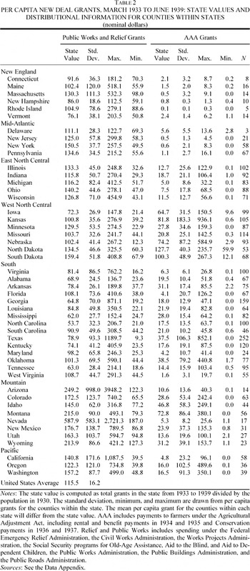
TABLE 2 PER CAPITA NEW DEAL GRANTS, MARCH 1933 TO JUNE 1939: STATE VALUES AND DISTRIBUTIONAL INFORMATION FOR COUNTIES WITHIN STATES (nominal dollars)
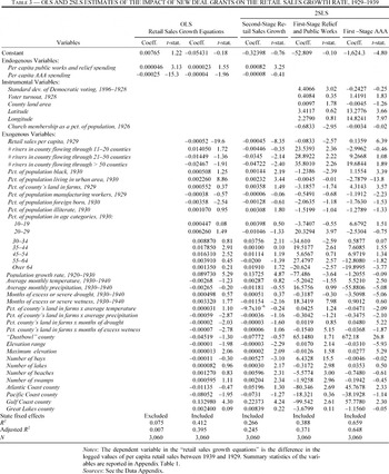
TABLE 3 OLS AND 2SLS ESTIMATES OF THE IMPACT OF NEW DEAL GRANTS ON THE RETAIL SALES GROWTH RATE, 1929–1939
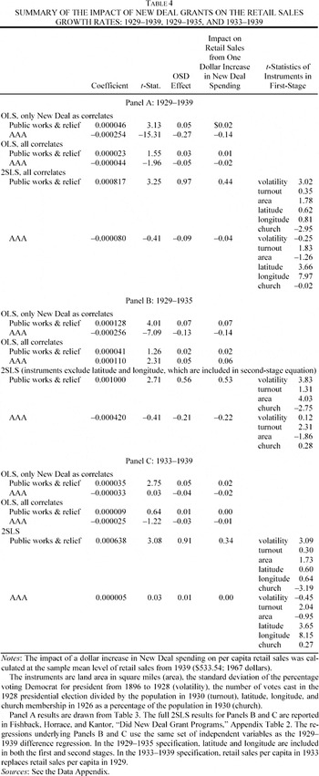
TABLE 4 SUMMARY OF THE IMPACT OF NEW DEAL GRANTS ON THE RETAIL SALES GROWTH RATES: 1929–1939, 1929–1935, AND 1933–1939
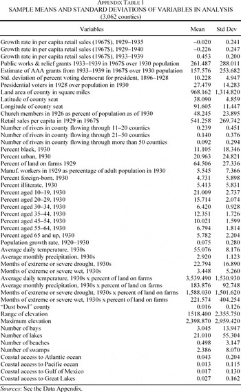
APPENDIX TABLE 1 SAMPLE MEANS AND STANDARD DEVIATIONS OF VARIABLES IN ANALYSIS (3,062 counties)
 You have Access
- 111
- Cited by