
 ⟨Θ⟩V,t
 ⟨wθ⟩V,t





1. Introduction
Convective flows in globally rotating reference frames are central to many problems in astrophysics and geophysics (Miesch Reference Miesch2005; Roberts Reference Roberts2015). In convective systems, buoyancy fluxes may originate at boundaries, as in canonical Rayleigh–Bénard convection (RBC), or be sustained by volumetric internal heating, as in internally heated convection (IHC). Although rotating RBC has been extensively characterised (Kunnen Reference Kunnen2021; Ecke & Shishkina Reference Ecke and Shishkina2023), rotating IHC has received limited investigation (Roberts Reference Roberts1965; Jones et al. Reference Jones, Soward and Mussa2000; Kaplan et al. Reference Kaplan, Schaeffer, Vidal and Cardin2017; Lin & Jackson Reference Lin and Jackson2021; Hadjerci et al. Reference Hadjerci, Bouillaut, Miquel and Gallet2024), especially in the plane layer geometry (Arslan Reference Arslan2024; Ostilla-Mónico & Arslan Reference Ostilla-Mónico and Arslan2025). In RBC, it has been demonstrated that rapid rotation gives rise to the quasi-geostrophic (QG) flow regimes (Charney Reference Charney1948), where the Coriolis force dominates buoyancy effects, balances the pressure gradient at leading order, and organises the flow into columnar structures aligned with the rotation axis. Above the rotation-suppressed onset of convection (Chandrasekhar Reference Chandrasekhar2013), increasing buoyancy transitions the flow morphology from Taylor columns to plumes, and eventually to geostrophic turbulence before the buoyancy effects dominate (Sprague et al. Reference Sprague, Julien, Knobloch and Werne2006; Julien et al. Reference Julien, Rubio, Grooms and Knobloch2012; King et al. Reference King, Stellmach and Aurnou2012; Aguirre Guzmán et al. Reference Aguirre Guzmán, Madonia, Cheng, Ostilla-Mónico, Clercx and Kunnen2022; Song et al. Reference Song, Shishkina and Zhu2024).
Rapidly rotating IHC is relevant to the dynamics of liquid alloys in planetary cores driven thermally or compositionally by radiogenic heating, secular cooling (Nimmo Reference Nimmo2015), and the exsolution of light elements (Badro et al. Reference Badro, Siebert and Nimmo2016; O’Rourke & Stevenson Reference O’Rourke and Stevenson2016), as well as to subsurface oceans on icy moons that are subject to tidal heating (Nimmo Reference Nimmo2018). In many of these contexts, direct numerical simulations and laboratory experiments cannot reach the appropriate parameter regimes (Cardin & Olson Reference Cardin and Olson2015; Christensen & Wicht Reference Christensen and Wicht2015). The principal difficulty lies in reaching the Ekman number (
 $E$
) and Rayleigh number (
 $R$
) required to reproduce geostrophic turbulence, where
 $E$
measures the ratio of the rotation period to the viscous diffusion time scale, and
 $R$
measures the destabilising effect of heating relative to diffusion. For instance, the Ekman number is approximately
 $10^{-15}$
in the Earth’s liquid outer core (De Wijs et al. Reference De Wijs, Kresse, Vočadlo, Dobson, Alfe, Gillan and Price1998),
 $10^{-13}$
in Mercury (Seuren et al. Reference Seuren, Triana, Rekier, Barik and Van Hoolst2023), and possibly
 $10^{-15}$
in early Mars (Dietrich & Wicht Reference Dietrich and Wicht2013). Given that convection requires a Rayleigh number at least as large as
 $E^{-4/3}$
(Chandrasekhar Reference Chandrasekhar2013; Arslan Reference Arslan2024),
 $R$
is at least of the order of
 $10^{17}$
and
 $10^{20}$
for these planetary bodies. Due to the
 $E$
-dependence of the maximum allowable time steps in computation (Julien et al. Reference Julien, van Kan, Miquel, Knobloch and Vasil2025), and to mechanical strength limitations in laboratory experiments, studies of geostrophic turbulence are currently restricted to
 $E\gtrsim 10^{-8}$
(Cheng et al. Reference Cheng, Madonia, Aguirre Guzmán and Kunnen2020; Song et al. Reference Song, Shishkina and Zhu2024). Moreover, the nonlinearity of the Navier–Stokes equations suggests that observations derived from a limited number of simulations may not accurately represent the systems’ large-scale behaviour.
Rigorous analysis of the governing partial differential equations (PDEs) provides an alternative route to insight. An approach first developed by Doering and Constantin, called the background field method (Doering & Constantin Reference Doering and Constantin1992, Reference Doering and Constantin1994, Reference Doering and Constantin1996; Constantin & Doering Reference Constantin and Doering1995), obtains bounds on long-time averages of diagnostic quantities in incompressible flows, determining how turbulent statistics depend on control parameters beyond the observable regime (Fantuzzi et al. Reference Fantuzzi, Arslan and Wynn2022). The method relies on two key ideas. First, instead of optimising a mean quantity over exact PDE solutions, one considers a broader set of incompressible flows constrained only by integral balances such as energy and flux conservation. Second, the flow is decomposed into fluctuations and an arbitrary steady background field that satisfies the boundary conditions. By prescribing the geometry of this background field, the original variational problem over the full state space is reduced to an optimisation over the parameters of the background field. The resulting bounds depend on the chosen function, and are valid provided that a quadratic form termed the spectral constraint is non-negative. This method has been demonstrated to be a special case of the auxiliary functional method (Chernyshenko et al. Reference Chernyshenko, Goulart, Huang and Papachristodoulou2014; Chernyshenko Reference Chernyshenko2022) with quadratic functionals, in which bounded functionals encode the constraints from dynamics, and the background field serves as a perturbation of an energy norm.
In the present work, we employ auxiliary functionals to investigate a new model of rapidly rotating convection driven by internal heating. We consider a uniformly heated Boussinesq fluid confined between stress-free, isothermal horizontal parallel plates, with gravity directed vertically downwards, parallel to the axis of rotation. The principal quantities characterising mean dissipation and energy transport at statistical equilibrium are the mean temperature and convective heat flux, each averaged over the volume and a sufficiently long time (Goluskin Reference Goluskin2016). These quantities are not a priori related, in contrast to RBC, and can depend on
 $R$
and
 $E$
, as well as the Prandtl number
 $\textit{Pr}$
, defined as the ratio of viscous to thermal diffusivity, and the height to length ratio of the domain. Previous studies applying the auxiliary functional method have established rigorous bounds for non-rotating IHC (Lu et al. Reference Lu, Doering and Busse2004; Whitehead & Doering Reference Whitehead and Doering2011, Reference Whitehead and Doering2012; Arslan et al. Reference Arslan, Fantuzzi, Craske and Wynn2023; Arslan & Rojas Reference Arslan and Rojas2025). Bounds for rotating IHC have been derived under no-slip boundary conditions (Arslan Reference Arslan2024). However, if
 $E\lesssim R^{-2}$
, then the bounds on both mean temperature and mean convective heat flux are independent of
 $E$
. As shown in table 1 of Arslan (Reference Arslan2024), bounds are established only for rotationally affected IHC, which corresponds to transitional regimes between buoyancy- and rotation-dominated dynamics. Therefore, the
 $E$
and
 $R$
dependence in the limit of rapid rotation remains an open question. Moreover, no investigation has addressed rotating IHC with stress-free boundaries. Here, we prove the first bounds on the mean temperature and convective heat flux with respect to
 $R$
and
 $E$
in the regime of rapid rotation at infinite
 $\textit{Pr}$
.
A standard energy identity of the Navier–Stokes equation fails to capture the effects of the Coriolis force, therefore such bounds contain no information on this crucial addition to the momentum balance compared with the non-rotating case. To progress, rather than working with the standard Navier–Stokes equations, we derive a model inspired by the non-hydrostatic QG (NH-QG) model (Julien et al. Reference Julien, Knobloch and Werne1998), an asymptotically reduced PDE system valid for
 $E^{1/3}\ll 1$
. The NH-QG equations were first developed by Julien et al. (Reference Julien, Knobloch and Werne1998) for rapidly rotating RBC between stress-free parallel plates, have been used to probe geostrophic turbulence (Sprague et al. Reference Sprague, Julien, Knobloch and Werne2006; Julien et al. Reference Julien, Rubio, Grooms and Knobloch2012; Calkins et al. Reference Calkins, Hale, Julien, Nieves, Driggs and Marti2015), and show consistency with solutions of the full Navier–Stokes equations (van Kan et al. Reference van Kan, Julien, Miquel and Knobloch2025).
Rapid rotation suppresses vertical fluid motion, and induces an anisotropy between the horizontal length scale
 $L$
and the vertical scale
 $H$
, resulting in columnar structures, and reducing the system’s effective dimensionality (Gallet Reference Gallet2015). Leveraging this rotational constraint, the NH-QG equations introduce an anisotropic non-dimensionalisation in which
 ${L}=E^{1/3} H$
, a scaling motivated by linear stability theory (Chandrasekhar Reference Chandrasekhar2013; Arslan Reference Arslan2024). The model describes dynamics on the small scale
 $L$
where the horizontal and vertical velocities are comparable, while assuming rotation to be sufficiently rapid so that the leading-order forces remain in geostrophic balance on this scale. The derivation of the NH-QG model proceeds by decomposing the flow fields into horizontally averaged components and fluctuations, expanding them in powers of
 $E^{1/3}$
, and matching terms order by order. This procedure separates fast, small-scale fluctuations from the slow evolution of the mean fields, and results in a closed PDE system for the leading-order components of the vertical velocity
 $w$
, the vertical vorticity
 $\zeta$
, the horizontal stream function
 $\psi$
, the horizontally averaged temperature
 $\varTheta$
, and the temperature fluctuation
 $E^{1/3}\theta$
.
The proof of bounds can be further aided by working in the infinite Prandtl number limit. Bounds in this limit are relevant for compositionally driven convection (Jones Reference Jones2015), and provide constraints that can be smoothly extended to finite
 $\textit{Pr}$
cases (Wang & Whitehead Reference Wang and Whitehead2013; Tilgner Reference Tilgner2022). With
 $\textit{Pr} \to \infty$
, the momentum equation reduces to a forced Stokes flow, which acts as a diagnostic constraint improving the estimates on the spectral constraint, the central step in deriving rigorous bounds within the auxiliary functional method. For the case of rapidly rotating RBC with stress-free boundaries, Grooms & Whitehead (Reference Grooms and Whitehead2014) were able to analyse the Green’s function of the Stokes flow to control the spectral constraint and proved that the Nusselt number
 $\textit{Nu}$
, which measures the ratio of the mean heat flux to its conductive counterpart, satisfies
 $\textit{Nu}\lesssim R^3 E^{4}$
up to constants. Using a similar approach, Pachev et al. (Reference Pachev, Whitehead, Fantuzzi and Grooms2020) demonstrated
 $\textit{Nu} \lesssim R^2 E^2$
for no-slip boundary conditions, where the effects of Ekman pumping on the bulk flow are incorporated through modified boundary conditions (Julien et al. Reference Julien, Aurnou, Calkins, Knobloch, Marti, Stellmach and Vasil2016). The present work provides the first application of NH-QG rescaling and bounding methods to rapidly rotating IHC systems.
Before presenting the main results, we introduce the coordinate system and averaging operators. An anisotropic Cartesian coordinate system
 $(x, y, Z)$
is adopted, where
 $Z:= E^{1/3}z$
is a rescaled vertical coordinate, with
 $z$
denoting the vertical coordinate measured in the same length units as
 $x$
and
 $y$
. The rescaled coordinate encodes the rotation-induced anisotropy between horizontal and vertical length scales (Julien et al. Reference Julien, Knobloch and Werne1998), so that as
 $\partial _Z =E^{-1/3}\partial _z$
, the vertical and horizontal gradients of the flow fields are of the same order after rescaling. For any
 $f = f(x,y,Z,t)$
defined on the periodic domain
 $V=[0, L_x] \times [0, L_y] \times [0, 1]$
, the following averaging operators are defined:
 \begin{equation} \overline {f}(Z,t):= {\frac {1}{L_y L_x }\int _0^{L_y }\int _0^{L_x }f\,\mathrm{d}x\,\mathrm{d}y}, \end{equation}
 \begin{equation} \langle f \rangle _{V}(t):= {\int _0^1 \overline {f}\,\mathrm{d}Z}, \end{equation}
 \begin{equation} \langle f\rangle _{V,t}:=\limsup _{\tau \to \infty }\frac {1}{\tau }{\int _0^\tau \langle f \rangle _{V} \,\mathrm{d}t}. \end{equation}
These represent the horizontal average, the volume average, and the long-time and volume average, respectively. The principal quantities to be bounded, namely the mean temperature and mean convective heat flux, are then denoted by
 $\langle \varTheta \rangle _{V,t}$
and
 $\langle w \theta \rangle _{V,t}$
.
In this paper, we prove the following two results. First, the lower bound for the mean temperature is
 \begin{equation} \langle \varTheta \rangle _{V,t}\gtrsim 0.66 E^{-1}R^{-3/4}, \end{equation}
up to second-order corrections, for
 $R\geq 19.2 E^{-4/3}$
. We also show that the flow remains purely conductive, with
 $\langle \varTheta \rangle _{V,t}=1/12$
for
 $R\leq 5.82 E^{-4/3}$
, where the threshold provides a lower bound for the nonlinear critical Rayleigh number. For the intermediate range
 $5.82E^{-4/3}\lt R\lt 19.2 E^{-4/3}$
, bounds are established as functions of
 $R$
and
 $E$
where terms with different scalings contribute at comparable orders.
The second result is the upper bound on the mean convective heat flux,
 \begin{equation} \langle {w\theta }\rangle _{V,t}\lesssim 0.04E^{4/5}R^{3/5}-0.25 \end{equation}
for
 $R\geq 30.2 E^{-4/3}$
. Furthermore, we show that
 $\langle {w\theta }\rangle _{V,t}=0$
for
 $R\leq 3.50 E^{-4/3}$
, and it is bounded above by a multi-scaling function of
 $R$
and
 $E$
for
 $3.50 E^{-4/3}\lt R\lt 30.2E^{-4/3}$
.
The remainder of the paper is organised as follows. In § 2, we introduce the reduced model for rapidly rotating IHC, with the derivation of the governing equations detailed in Appendix A within the NH-QG framework. After defining the system, we state rigorous bounds on
 $\langle \varTheta \rangle _{V,t}$
and
 $\langle w\theta \rangle _{V,t}$
as theorems, and demonstrate the relevance of these quantities for characterising the dynamics. The lower bound for
 $\langle \varTheta \rangle _{V,t}$
and the upper bound for
 $\langle w\theta \rangle _{V,t}$
are proved in §§ 3 and 4, respectively. To complement the analysis, we present numerical optimisation results for both quantities in § 5. Finally, § 6 provides a discussion and summary of the present work. Appendix B establishes the boundedness of the auxiliary functional used in this study when evaluated along solutions of the governing equations, and Appendix C presents a linear stability analysis of the conduction state. For notation, we use
 $\|{\cdot }\|_2$
and
 $\|{\cdot}\|_{\infty }$
for the
 $L^2$
and
 $L^\infty$
norms of a function over
 $Z\in [0,1]$
, and
 $({\cdot })'$
denotes differentiation with respect to
 $Z$
.
2. Preliminaries
2.1. Configuration and governing equations
(a) A schematic diagram of rotating IHC between two isothermal parallel plates with stress-free boundary conditions. The uniform heating source is denoted by
 $S$
, and
 $H$
is the separation between the two plates in the direction of gravity,
 $g$
. Horizontal periodicities are
 $L_x H$
and
 $L_y H$
. The convection is subject to global rotation
 $\varOmega$
. Without loss of generality, the boundary temperature is set to
 $T_b = 0$
. Circles indicate flow structures with a characteristic vertical scale
 $H$
and horizontal scale
 $E^{1/3}H$
. (b) The same flow structures shown in dimensionless coordinates. The vertical and horizontal length units are
 $H$
and
 $E^{1/3}H$
, respectively, with
 $E\ll 1$
.

As illustrated in figure 1(a), we consider an incompressible fluid between two parallel plates separated by a distance
 $H$
with horizontal periodicities
 $L_x H$
and
 $L_y H$
. The fluid is characterised by reference density
 $\rho$
, thermal diffusivity
 $\kappa$
, kinematic viscosity
 $\nu$
, specific heat
 $c_p$
, and thermal expansivity
 $\alpha$
. Convection is driven by a uniform volumetric heat source
 $S$
under a constant gravitational acceleration
 $-g \hat {\boldsymbol{z}}$
. The system rapidly rotates about the vertical axis with constant angular velocity
 $\varOmega$
.
To describe rapid rotation, we use an asymptotically reduced set of equations to model the convection of a Boussinesq fluid in the limit of infinite Prandtl number
 $\textit{Pr}$
. The Prandtl number is defined in (2.1) and is the ratio of viscous to thermal diffusivity. The other control parameters are the Rayleigh number
 $R$
and Ekman number
 $E$
, where
 $R$
quantifies the destabilising effect of heating to the stabilising effect of diffusion, and
 $E$
gives the effect of inertia compared to rotation. These control parameters are defined as
 \begin{equation} R = \frac {\alpha g S H^5}{\rho c_p \nu \kappa ^2}, \quad E = \frac {\nu }{2\varOmega H^2}, \quad \textit{Pr}= \frac {\nu }{\kappa }. \end{equation}
An additional key control parameter characterising the dynamics is the reduced Rayleigh number (Julien et al. Reference Julien, Knobloch and Werne1998) measuring the degree of supercriticality:
 \begin{equation} \mathcal{R} = R E^{4/3}. \end{equation}
To non-dimensionalise, we choose the vertical length scale to be
 $H$
, and the horizontal length scale to be
 $E^{1/3} H$
. The effect of this anisotropic non-dimensionalisation on rotation-constrained columnar flow structures is illustrated in figure 1(b). The time and temperature scales are
 $E^{2/3} H^2 / \kappa$
and
 $S H^2/\rho c_p \kappa$
, respectively. Then in the asymptotic limit of rapid rotation, the equations for convection at infinite
 $\textit{Pr}$
(see Appendix A for a derivation) are
 \begin{equation} \partial _Z\psi ={\mathcal{R}}\theta +{\nabla} _h^2w, \end{equation}
 \begin{equation} -\partial _Zw={\nabla} _h^2\zeta , \end{equation}
 \begin{equation} \zeta ={\nabla} _h^2\psi , \end{equation}
 \begin{equation} \partial _t\theta + J\left [\psi ,\theta \right ]+w\partial _Z \varTheta ={\nabla} _h^2\theta , \end{equation}
 \begin{equation} E^{-{2}/{3}}\,\partial _t \varTheta +\partial _Z(\overline {w\theta })=\partial _Z^2 \varTheta +1. \end{equation}
Here,
 $J[\psi ,{\cdot }\,]:= \partial _x\psi \,\partial _y({\cdot }) - \partial _y\psi \,\partial _x({\cdot })$
,
 $\boldsymbol{\nabla} _h({\cdot }):= \hat {\boldsymbol{x}}\,\partial _x({\cdot })+\hat {\boldsymbol{y}}\,\partial _y({\cdot })$
and
 ${\nabla} _h^2 := \partial _x^2 + \partial _y^2$
denotes the horizontal Laplacian. Then
 $\psi (x,y,Z,t)$
is the horizontal streamfunction, with the horizontal velocity being
 $-\boldsymbol{\nabla} _h\times (\psi \hat {\boldsymbol{Z}})$
. Here,
 $w(x,y,Z,t)$
is the vertical velocity,
 $\zeta (x,y,Z,t)$
is the vertical vorticity,
 $\varTheta (Z,t)$
is the horizontally averaged temperature field, and
 $E^{1/3}\theta (x,y,Z,t)$
is the temperature anomaly relative to the horizontal average. It is noted that
 $w$
,
 $\zeta$
,
 $E^{1/3}\theta$
and
 $\varTheta$
represent the leading-order non-zero components of the corresponding fields in an asymptotic expansion in powers of
 $E^{1/3}$
, with the incompressibility condition satisfied by advection on higher-orders. If these variables are instead interpreted as the full fields, then (2.3a
)–(2.3e
) incur an error of
 $O(E^{1/3})$
. The total temperature field
 $T(x,y,Z,t)$
is approximated by
 \begin{align} T=\varTheta +E^{{1}/{3}}\theta . \end{align}
As demonstrated in Appendix A, the horizontal means of
 $w$
,
 $\zeta$
and
 $\psi$
vanish, while
 $\theta$
has zero horizontal mean by definition. Hence
 $\overline {\theta } = \overline {w} = \overline {\zeta } = \overline {\psi } = 0$
.
In the derivation of (2.3), the geostrophic balance is assumed to constitute the leading-order force balance throughout the domain, thereby excluding any boundary-layer effects (see Appendix A). For the physical consistency of the resulting PDEs, we impose stress-free mechanical boundary conditions. For the temperature, the isothermal boundary conditions
 $T=T_b$
are applied. Without loss of generality,
 $T_b$
is set to zero. The boundary conditions are thus given by
 \begin{equation} w=\partial _Z\zeta =\partial _Z\psi =\theta =\varTheta = 0\quad \mathrm{at}\ Z=0\ \mathrm{and}\ Z=1. \end{equation}
2.2. Main theorems
Having defined the governing equations and boundary conditions, here we state the two theorems proved in this work.
Theorem 1 (Lower bound on mean temperature).
On the domain
 $V=[0,E^{-1/3}L_x]\times [0,E^{-1/3}L_y]\times [0,1]$
, let
 $\omega,\psi,\theta : V\times [0,\infty ) \to \mathbb{R}$
and
 $\varTheta:[0,1]\times [0,\infty ) \to \mathbb{R}$
satisfy the model defined in (
2.3
), with periodic boundary conditions in
 $x$
and
 $y$
, and subject to the boundary conditions (
2.5
). Let
 $\langle \varTheta \rangle _{V,t}$
be the volume and long-time average of
 $\varTheta$
as defined by (
1.1c
). Then
 \begin{align} \langle \varTheta \rangle _{V,t}\geq \begin{cases} 1.13E^{-8/7}R^{-6/7}-1.61 E^{-12/7}R^{-9/7},&5.82 E^{-4/3}\leq R\lt 19.2E^{-4/3},\\[5pt] 0.66E^{-1}R^{-3/4}- 1.51E^{-2}R^{-3/2},& R\geq 19.2 E^{-4/3}, \end{cases} \end{align}
where
 $5.82 E^{-4/3}$
corresponds to a lower threshold for nonlinear instability of the flow. For
 $R\lt 5.82 E^{-4/3}$
, the conductive state is globally asymptotically stable, and
 $\langle \varTheta \rangle _{V,t}=1/12$
.
It is straightforward to verify that the lower bounds are positive for all
 $R$
over which the bounds hold.
Theorem 2 (Upper bound on mean heat flux).
On the domain
 $V=[0,E^{-1/3}L_x]\times [0,E^{-1/3}L_y]\times [0,1]$
, let
 $\omega,\psi,\theta : V\times [0,\infty ) \to \mathbb{R}$
and
 $\varTheta:[0,1]\times [0,\infty ) \to \mathbb{R}$
satisfy the model defined in (
2.3
), with periodic boundary conditions in
 $x$
and
 $y$
, and subject to the boundary conditions (
2.5
). Let
 $\langle w\theta \rangle _{V,t}$
be the volume and long-time average of
 $w\theta$
as defined by (
1.1c
). Then
 \begin{align} \langle {w\theta }\rangle _{V,t}\leq \begin{cases} \begin{aligned} 0.01 E^{8/7}R^{6/7}-0.25 +0.57 E^{-4/7}R^{-3/7}-0.37E^{-8/7}R^{-6/7} , &\\[7pt] 3.50E^{-4/3}\leq R\lt 30.2E^{-4/3},&\\[7pt] 0.04E^{4/5}R^{3/5}-0.25- 0.15 E^{-4/5}R^{-3/5}+3.95E^{-8/5}R^{-6/5}, &\\[7pt] R\geq 30.2 E^{-4/3}.& \end{aligned} \end{cases} \end{align}
For
 $R\lt 3.50E^{-4/3}$
, the conductive state is globally asymptotically stable, and
 $\langle w\theta \rangle _{V,t}=0$
.
2.3. Quantities of interest
In this subsection, we demonstrate the relevance of the quantities for which we have stated bounds in Theorem1 and Theorem2. The mean temperature
 $\langle \varTheta \rangle _{V,t}$
quantifies the thermal dissipation and effective mixing of the fluid, while the mean convective heat flux
 $\langle {w\theta }\rangle _{V,t}$
quantifies the asymmetry in heat flux out of the domain due to convection. To see this, we multiply (2.3d
) and (2.3e
) by
 $\theta$
and
 $\varTheta$
, respectively, apply the spatial average (1.1b
), integrate by parts, and sum to obtain
 \begin{equation} \frac {E^{-{2}/{3}}}{2} \frac {\mathrm{d}}{\mathrm{d} t}\langle \varTheta ^2+E^{{2}/{3}}\theta ^2\rangle _{V}=-\langle \left |\boldsymbol{\nabla} _h \theta \right |^2+(\partial _Z \varTheta )^2\rangle _{V}+\langle \varTheta \rangle _{V}, \end{equation}
where the left-hand side represents the rate of change of the thermal energy density, while the first term on the right-hand side corresponds to the thermal dissipation rate. Further applying the long-time average yields the mean energy equilibrium
 \begin{equation} \langle \left |\boldsymbol{\nabla} _h \theta \right |^2+(\partial _Z \varTheta )^2\rangle _{V,t} = \langle \varTheta \rangle _{V,t}. \end{equation}
On the other hand, multiplying (2.3a
) and (2.3b
) by
 $w$
and
 $\psi$
, respectively, and proceeding similarly leads to the identity
 \begin{equation} \langle \zeta ^2+\left |\boldsymbol{\nabla} _h w\right |^2\rangle _{V,t} = {\mathcal{R}}\langle w\theta \rangle _{V,t}, \end{equation}
with the left-hand side representing the dissipation arising from velocity gradients. As can be seen in (2.9) and (2.10), the mean temperature and convective heat transport are non-negative, and this gives uniform lower bounds
 $\langle w \theta \rangle _{V,t} \geq 0$
and
 $ \langle \varTheta \rangle _{V,t} \geq 0$
. For a uniform upper bound on
 $\langle w \theta \rangle _{V,t}$
, we multiply (2.3e
) by
 $Z$
, and take the average (1.1c
). With
 $\mathcal{F}_T$
and
 $\mathcal{F}_B$
defined as the heat fluxes exiting through the top and bottom boundaries, this yields
 \begin{equation} \mathcal{F}_T:=\left . -\limsup _{\tau \rightarrow \infty }\frac {1}{\tau }\int ^{\tau }_0 \partial _Z \varTheta \right |_{Z=1} \mathrm{d}t =\frac {1}{2}+\langle w\theta \rangle _{V,t}, \end{equation}
 \begin{equation} \mathcal{F}_B:= \left . \limsup _{\tau \rightarrow \infty }\frac {1}{\tau }\int ^{\tau }_0 \partial _Z \varTheta \right |_{Z=0} \mathrm{d}t =\frac {1}{2}-\langle w\theta \rangle _{V,t}. \end{equation}
Given that the temperature within the domain is pointwise non-negative,
 $T \geq T_b=0$
with any deviation decaying exponentially in time (Arslan et al. Reference Arslan, Fantuzzi, Craske and Wynn2021), the heat fluxes are also signed, thus we infer that
 $\langle w\theta \rangle _{V,t} \leq 1/2$
. The uniform upper bound on the mean temperature is given by the conductive solution of the system (2.3) subject to (2.5), where the conductive temperature profile is
 \begin{equation} \varTheta _c=\frac {1}{2}Z(1-Z). \end{equation}
It follows that
 $\langle \varTheta \rangle _{V,t} \leq \langle \varTheta _c \rangle _{V}=1/12$
, with a proof analogous to that in Goluskin & Spiegel (Reference Goluskin and Spiegel2012).
2.4. Horizontal Fourier domain
Before presenting the framework for deriving rigorous bounds on
 $\langle {\varTheta }\rangle _{V,t}$
and
 $\langle {w\theta }\rangle _{V,t}$
, we introduce a Fourier expansion in the horizontal direction. Let
 $\mathcal{K}$
denote the set of all non-zero horizontal wavevectors
 $\boldsymbol{k}=k_x\hat {\boldsymbol{x}}+k_y\hat {\boldsymbol{y}}$
permitted by the dimensionless periods
 $E^{-1/3}L_x$
and
 $E^{-1/3}L_y$
. For any scalar field denoted generically by
 $f$
, we write
 \begin{align} f=\overline {f}+\sum _{\boldsymbol{k}\in \mathcal{K}}{f}_{\boldsymbol{k}}(Z,\,t)\,\mathrm{e}^{\mathrm{i} \left (k_xx+k_yy\right )}, \end{align}
where
 \begin{align} \mathcal{K} = \left \{ (k_x,k_y) = E^{1/3}\left (\frac {2\pi m}{L_x}, \frac {2\pi n}{L_y}\right )\Bigg | (m,n) \in \mathbb{Z}^2 \,\& \, (m,n)\neq (0,0) \right \}\!. \end{align}
Therein,
 ${f}_{\boldsymbol{k}}$
represent the Fourier coefficients. Since
 $f$
is real-valued, the coefficients satisfy
 ${f}_{\boldsymbol{k}}^{*}={f}_{-\boldsymbol{k}}$
, with
 $({\cdot })^{*}$
denoting complex conjugation. Under the expansion (2.13b
), the combination of (2.3a
)–(2.3c
) yields a diagnostic relation between
 $w_{\boldsymbol{k}}$
and
 $\theta _{\boldsymbol{k}}$
,
 \begin{equation} \theta _{\boldsymbol{k}}=\frac {1}{{\mathcal{R}}}\left (k^2 {w}_{\boldsymbol{k}}-\frac {1}{k^4}\,\partial _Z^2 {w}_{\boldsymbol{k}}\right )\!, \end{equation}
in which
 $k=\sqrt {k_x^2+k_y^2}$
is the magnitude of each wavevector.
3. Bounds for mean temperature
 $\langle \varTheta \rangle _{V,t}$

3.1. Bounding framework
To bound
 $\langle \varTheta \rangle _{V,t}$
, we follow the auxiliary functional method (Fantuzzi et al. Reference Fantuzzi, Arslan and Wynn2022), which is based on the observation that for any bounded functional
 $\mathcal{V}\{\varTheta ,\theta \}$
along the solutions of the governing equations (2.3), the time derivative of
 $\mathcal{V}\{\varTheta ,\theta \}$
has zero long-time average. Moreover, the time average of a quantity is bounded from below by its pointwise infimum, so that where
 $\mathcal{V}$
is independent of spatial coordinates,
 \begin{equation} \langle \varTheta \rangle _{V,t}=\limsup _{\tau \rightarrow \infty }\frac {1}{\tau }\int ^{\tau }_0 \langle \varTheta \rangle _{V}-\frac {\mathrm{d}{\mathcal{V}}}{\mathrm{d}t}\,\mathrm{d}t\geq \inf \left (\langle \varTheta \rangle _{V}-\frac {\mathrm{d}{\mathcal{V}}}{\mathrm{d}t}\right )\geq B_{1}. \end{equation}
Therefore,
 $B_{1}$
, which may ultimately be shown to be a function of
 $R$
and
 $E$
, serves as a lower bound for
 $\langle \varTheta \rangle _{V,t}$
, provided that there exists an auxiliary functional
 $\mathcal{V}\{\varTheta ,\theta \}$
such that
 \begin{equation} Q:= \langle \varTheta \rangle _{V}-\frac {\mathrm{d}\mathcal{V}}{\mathrm{d}t}-B_{1}\geq 0. \end{equation}
We consider the quadratic auxiliary functional
 \begin{equation} \mathcal{V}\{\varTheta ,\theta \} = \frac {\beta }{2} \big \langle \theta ^2+E^{-{2}/{3}}\varTheta ^2 \big \rangle _{V}-E^{-{2}/{3}}\left \langle \phi \,\varTheta \right \rangle _{V}, \end{equation}
where
 $\beta \gt 0$
is referred to as the balance parameter, and we call
 $\phi =\phi (Z)$
the background field, although in most prior work,
 $\phi /\beta$
is typically referred to as the background field. The boundedness of
 $\mathcal{V}\{\varTheta ,\theta \}$
along solutions of (2.3) is demonstrated in Appendix B. Here,
 $\phi$
is piecewise differentiable with a square-integrable derivative, and satisfies the homogeneous boundary conditions
 \begin{equation} \phi (0)=0,\quad \phi (1)=0. \end{equation}
Now, we show that condition (3.2) is enforced by a
 $B_{1}$
value given by an appropriate choice of
 $\phi$
, and that the resulting
 $B_1$
is a valid lower bound on
 $\langle \varTheta \rangle _{V,t}$
, provided that an associated quadratic form is non-negative.
Proposition 1 (Bound on
 $\langle \varTheta \rangle _{V,t}$
). For a given background field
 $\phi :[0,1]\rightarrow \mathbb{R}$
satisfying the boundary conditions (
3.4
), the scalar
 $B_{1}$
provides a lower bound on the mean temperature, where
 \begin{equation} B_{1}:=\int _0^1 \phi -\frac {1}{4}\phi '^2\,\mathrm{d}Z, \end{equation}
provided that the so-called spectral constraint is also satisfied:
 \begin{equation} Q_{\boldsymbol{k}}\left \{w,\phi \right \}\geq 0,\quad \forall k\gt 0,\quad \forall \! \left .w \,\right | \,{w}(0)={w}(1)=0, \end{equation}
in which
 \begin{equation} Q_{\boldsymbol{k}}:= k^6\,\|{w}_{\boldsymbol{k}}\|^2_2+2\,\|{w}^{\prime }_{\boldsymbol{k}}\|^2_2+\frac {1}{k^6}\|{w}^{\prime \prime }_{\boldsymbol{k}}\|^2_2+{\mathcal{R}}\int _0^1\phi '\left (k^2\left |w_{\boldsymbol{k}}\right |^2-\frac {1}{k^4}\,{\rm Re}\{{w}^{\prime \prime }_{\boldsymbol{k}}{w}^*_{\boldsymbol{k}}\}\right ) \mathrm{d}Z. \end{equation}
Proof.
From (2.3d
)–(2.3e
), we start by calculating the Lie derivative of
 $\mathcal{V}$
in (3.3). By integration by parts, use of the boundary conditions (2.5) and fixing
 $\beta =1$
, we get that
 \begin{equation} \frac {\mathrm{d}\mathcal{V}}{\mathrm{d}t} = -\big \langle |\boldsymbol{\nabla} _h \theta |^2 + | \varTheta '|^2 + \phi ' w\theta + (Z- \phi ') \varTheta ' + \phi \big \rangle _{V}. \end{equation}
We proceed by substituting (3.8) into the definition of
 $Q$
in (3.2), and applying the horizontal Fourier expansion (2.13b
) to
 $w$
and
 $\theta$
. This yields the decomposition
 \begin{equation} Q\{\varTheta ,w,\theta \}=Q_0\{\varTheta \}+\sum _{\boldsymbol{k}\in \mathcal{K}}Q_{\boldsymbol{k}}\{w_{\boldsymbol{k}},\theta _{\boldsymbol{k}}\}, \end{equation}
where
 \begin{align} Q_0=-B_{1}+\int _0^1 (|\varTheta '|^2-\phi ' \varTheta ' +\phi) \,\mathrm{d}Z, \end{align}
 \begin{align} Q_{\boldsymbol{k}}= k^2\,\| {\theta }_{\boldsymbol{k}}\|^2_2+\int _0^1 \phi ' \,{\rm Re}\{ {w}_{\boldsymbol{k}} {\theta }_{\boldsymbol{k}}^*\}\, \mathrm{d}Z. \end{align}
Condition (3.2) is satisfied by requiring
 $Q_0 \geq 0$
and
 $Q_{\boldsymbol{k}} \geq 0$
independently. Noting that
 $Q_0$
is convex in
 $\varTheta '$
, we solve the associated Euler–Lagrange equation with respect to
 $\varTheta$
, subject to Dirichlet boundary conditions. The non-negativity condition on
 $Q_0$
is satisfied in the worst case by
 \begin{equation} B_{1} = \inf _{ \substack {\varTheta (Z) \\ \varTheta (0)= \varTheta (1)=0 } } \int _0^1(|\varTheta ' |^2-\phi '\varTheta ' +\phi) \,\mathrm{d}Z, \end{equation}
with the minimiser given by
 \begin{equation} \varTheta '_{\textit{opt}}=\frac {\phi '}{2}. \end{equation}
Then substituting (3.12) into (3.11) gives the form (3.5).
Next, in (3.10b
), we eliminate the spectral coefficient
 $\theta _{\boldsymbol{k}}$
using the diagnostic relation (2.14), and rearrange through integration by parts to obtain
 \begin{align} \begin{aligned} Q_{\boldsymbol{k}}={}&\frac {1}{{\mathcal{R}}^2}\left (k^6\,\|{w_{\boldsymbol{k}}}\|^2_2+2\,\|{w_{\boldsymbol{k}}^{\prime }}\|^2_2+\frac {1}{k^6}\|{w_{\boldsymbol{k}}^{\prime \prime }}\|^2_2\right ) \\ &{}+\frac {1}{{\mathcal{R}}}\int _0^1\phi '\left (k^2\left |w_{\boldsymbol{k}}\right |^2-\frac {1}{k^4}\,{\rm Re}\{{w_{\boldsymbol{k}}^{\prime \prime }}{w_{\boldsymbol{k}}}^*\}\right ) \mathrm{d}Z. \end{aligned} \end{align}
The condition
 $Q_{\boldsymbol{k}} \geq 0$
for all
 $\boldsymbol{k}$
is satisfied by the spectral constraint.
Maximising (3.5) over all choices of
 $\phi$
subject to the spectral constraint yields the largest lower bound attainable within our framework. This optimisation problem is convex, and while analytically intractable, can be numerically solved. To obtain explicit bounds with rigorous parametrisation, here we focus on proving Theorem1 by constructing a suboptimal ansatz for
 $\phi$
, but present results of the numerical optimisation, where no specific form of
 $\phi$
is prescribed, in § 5.
If
 $L_x$
and
 $L_y$
were prescribed, then it would only be necessary for
 $Q_{\boldsymbol{k}}\geq 0$
to hold for the corresponding subset of positive wavenumbers, in order for
 $B_{1}$
to be a valid bound. Here, we require
 $Q_{\boldsymbol{k}}\geq 0$
for every positive
 $k$
. The resulting bounds are thereby valid for arbitrary horizontal periods, and for flow structures with arbitrary horizontal length scales, provided that (2.3) remains representative for the dynamics.
3.2. Ansatz
We restrict
 $\phi (Z)$
to take the form
 \begin{equation} \phi := \begin{cases} ({A}/{\delta ^2})Z\left (2\delta -Z\right ), &0\leq Z\leq \delta ,\\[5pt] A,&\delta \lt Z\lt 1-\delta ,\\[5pt] ({A}/{\delta ^2})\left (1-Z\right )\left (2\delta +Z-1\right ), &1-\delta \leq Z\leq 1. \end{cases} \end{equation}
Here,
 $\phi (Z)$
is characterised by boundary layers of thickness
 $\delta \in (0, 1/2]$
at the top and bottom of the layer, and by the amplitude parameter
 $A\gt 0$
specifying the bulk value of
 $\phi$
(figure 2).
The choice of a background field with quadratic boundary layers and a constant interior is motivated by the following considerations. First, it renders the sign-indefinite integral in (3.7) identically zero in the bulk. Second, as will be demonstrated in § 3.4, the maximal lower bound attainable with (3.14) is exactly
 $1/12$
when
 $\mathcal{R}$
is below a certain threshold. This value is achieved with the choice
 $A=1/4$
and
 $\delta = 1/2$
, for which the optimiser
 $\varTheta _{\textit{opt}}$
in (3.12) is exactly equivalent to the conductive state (2.12), and the spectral constraint becomes equivalent to a sufficient condition for nonlinear stability based on the energy method. This is only possible by using the quadratic boundary layers in
 $Z$
.
A sketch of the background profile (3.14) featuring quadratic boundary layers.

Substituting (3.14) into (3.5) and (3.7) leads to
 \begin{equation} B_{1}=A\left (1-\frac {2\delta }{3}\right )-\frac {2A^2}{3\delta }, \end{equation}
along with
 \begin{equation} Q_{\boldsymbol{k}}= \underbrace { k^6\,\|{w}_{\boldsymbol{k}}\|_2^2+2\,\|{w}^{\prime }_{\boldsymbol{k}}\|_2^2+\frac {1}{k^6}\,\|{w}^{\prime \prime }_{\boldsymbol{k}}\|_2^2 }_{P} +\frac {2{\mathcal{R}} A}{\delta ^2}\left (I_B -I_T\right )\!, \end{equation}
in which
 \begin{align} I_B= \int _0^\delta \left (\delta -Z \right )\left ( k^2\,|{w}_{\boldsymbol{k}}|^2-\frac {1}{k^4}\,{\rm Re}\{{w}^{\prime \prime }_{\boldsymbol{k}}{w}^*_{\boldsymbol{k}} \} \right )\mathrm{d}Z, \\[-12pt]\nonumber \end{align}
 \begin{align} I_T=\int _{1-\delta }^{1} \left (Z-1+\delta \right )\left ( k^2|{w}_{\boldsymbol{k}}|^2-\frac {1}{k^4}\,{\rm Re}\{{w}^{\prime \prime }_{\boldsymbol{k}}{w}^*_{\boldsymbol{k}} \} \right )\mathrm{d}Z. \end{align}
3.3. Sufficient conditions for the spectral constraint
As a central step in proving Theorem1 using Proposition1, we establish in this subsection a closed-form sufficient condition on
 $\delta$
and
 $A$
, from
 $\phi$
given by (3.14), that guarantees that the spectral constraint (3.6) is satisfied. This amounts to ensuring the non-negativity of (3.16) for all
 $k\gt 0$
. To this end, we first present two lemmas, each providing a sufficient condition for the non-negativity of (3.16): one for the range
 $k\geq k_c$
, and another for
 $0\lt k\leq k_c$
, with
 $k_c\gt 0$
being an arbitrary threshold wavenumber. Then, by reconciling the ranges of large and small wavenumbers, we obtain a single condition to satisfy the spectral constraint.
3.3.1. For large wavenumbers
$k\geq k_c$

Lemma 1 (Sufficient conditions for
 $Q_{\boldsymbol{k}}\geq 0$
, large
 $k$
). Let
 $Q_{\boldsymbol{k}}$
be specified by (
3.16
) and (
3.17
), and let
 $k_c\gt 0$
be a lower threshold wavenumber. Suppose that
 $A\gt 0$
satisfies
 \begin{equation} {\mathcal{R}} A\leq \sqrt {\frac {2}{5}}\,k_c. \end{equation}
Then
 $Q_{\boldsymbol{k}}\geq 0$
for all
 $k\geq k_c$
.
Proof.
We prove the lemma by constructing a lower bound on
 $Q_{\boldsymbol{k}}$
that is non-negative under the condition (3.18). The contribution of
 $\phi$
from (3.14) to
 $I_B$
and
 $I_T$
, as defined in (3.17a
) and (3.17b
), is symmetric. Hence apart from deriving a lower bound on
 $P$
, which has been defined in (3.16), we only prove upper and lower bounds on
 $I_B$
, since the identical estimates hold for
 $I_T$
. Using the boundary condition
 $w_{\boldsymbol{k}}(0)=0$
and integrating by parts, the
 $O(k^{-4})$
term in (3.17a
) can be written as
 \begin{equation} \begin{aligned} \int ^{\delta }_0 (\delta - Z)\,{{\rm Re}}\{ w''_{\boldsymbol{k}}w_{\boldsymbol{k}}^* \}\, \mathrm{d}Z &= \int ^{\delta }_0 \frac {1}{2} \left (\left |w_{\boldsymbol{k}}\right |^2 \right )' - (\delta -Z)\, |w'_{\boldsymbol{k}}|^2\, \mathrm{d}Z \\ &= \frac 12 |w_{\boldsymbol{k}}(\delta )|^2 - \int ^{\delta }_0 (\delta - Z )\,|w'_{\boldsymbol{k}}|^2\, \mathrm{d}Z. \end{aligned} \end{equation}
Then
 \begin{equation} \begin{aligned} I_B &= \int ^{\delta }_0 (\delta -Z) \left (k^2\, |w_{\boldsymbol{k}}|^2 + \frac {1}{k^4} |w'_{\boldsymbol{k}}|^2 \right ) \mathrm{d}Z -\frac {1}{2k^4}|w_{\boldsymbol{k}}(\delta )|^2 \\ &\leq \int ^{\delta }_0 (\delta -Z) \left (k^2\, |w_{\boldsymbol{k}}|^2 + \frac {1}{k^4} |w'_{\boldsymbol{k}}|^2 \right ) \mathrm{d}Z. \end{aligned} \end{equation}
Next, using that
 $|w|\leq \|w\|_\infty$
and
 $\left |w^{\prime }\right |\leq \|w^{\prime }\|_\infty$
, we get that
 \begin{equation} I_B\leq \int _{0}^{\delta } \left (\delta -Z\right )\left (k^2\,\|w_{\boldsymbol{k}}\|_\infty ^2+\frac {1}{k^4}\|w'_{\boldsymbol{k}}\|_\infty ^2\right )\mathrm{d}Z=\frac {\delta ^2}{2}\left (k^2\,\|w_{\boldsymbol{k}}\|_\infty ^2+\frac {1}{k^4}\|w'_{\boldsymbol{k}}\|_\infty ^2\right )\!. \end{equation}
On the other hand, the fundamental theorem of calculus implies
 \begin{equation} \left |w_{\boldsymbol{k}}(Z)\right |=\left |\int _0^Z w'_{\boldsymbol{k}}(\eta )\,\mathrm{d}\eta \right |\leq \int _0^Z \|w'_{\boldsymbol{k}}\|_{\infty }\,\mathrm{d}\eta =Z\,\|w'_{\boldsymbol{k}}\|_{\infty }, \end{equation}
hence from the identity in (3.20),
 $I_B$
is lower bounded as
 \begin{equation} I_B\geq -\frac {1}{2k^4}\left |w_{\boldsymbol{k}}(\delta )\right |^2\geq -\frac {\delta ^2}{2k^4}\|w'_{\boldsymbol{k}}\|_{\infty }^2. \end{equation}
Since
 $I_T$
is upper bounded by the right-hand side of (3.21), inserting (3.21) and (3.23) into (3.16) yields a sufficient condition for
 $Q_{\boldsymbol{k}}\geq 0$
:
 \begin{equation} P - {\mathcal{R}} A \left (k^2\,\|w_{\boldsymbol{k}}\|_\infty ^2+\frac {2}{k^4}\|w'_{\boldsymbol{k}}\|_\infty ^2\right ) \geq 0. \end{equation}
To proceed, we estimate
 $P$
from below. Denote
 $w_{\boldsymbol{k}}(Z)=w_{r}(Z)+\mathrm{i}\,w_{i}(Z)$
, with
 $w_r$
and
 $w_i$
being real functions. As
 $w_{\boldsymbol{k}}(1)=w_{\boldsymbol{k}}(0)=0$
, the mean value theorem guarantees the existence of points
 $Z_i \in [0,1 ]$
such that
 ${w}^{\prime }_{r}(Z_r) ={w}^{\prime }_{i}(Z_i)=0$
. Hence for any
 $Z\in [0,1]$
, the pointwise estimate holds that
 \begin{equation} \begin{aligned} \left |w'_{\boldsymbol{k}}(Z)\right |^2&=\left |w'_{r}(Z)\right |^2+\left |w'_{i}(Z)\right |^2\\ &=2\int _{Z_r}^Z {w_{r}^{\prime }}(\eta )w_{r}^{\prime \prime }(\eta )\,\mathrm{d}\eta +2\int _{Z_i}^Z {w_{i}^{\prime }}(\eta )w_{i}^{\prime \prime }(\eta )\,\mathrm{d}\eta \\ &\leq 2\int _0^1 (\left |w_r'(\eta )\right |\left |w_{r}^{\prime \prime }(\eta )\right |+\left |w_i'(\eta )\right |\left |w_{i}^{\prime \prime }(\eta )\right |)\, \mathrm{d}\eta . \end{aligned} \end{equation}
Taking the supremum over
 $Z$
and applying the Cauchy–Schwarz inequality then gives
 \begin{equation} \begin{aligned} \|w'_{\boldsymbol{k}}\|_{\infty }^{2}&=\sup _{Z}\left |w_{\boldsymbol{k}}^{\prime }(Z)\right |^2 \leq 2\left (\|w_r'\|_2\,\|w_r''\|_2+\|w_i'\|_2\,\|w_i''\|_2 \right )\\ &\leq 2\,\sqrt {\|w_r'\|_2^2+\|w_i'\|_2^2}\,\sqrt {\|w_r''\|_2^2+\|w_i''\|_2^2}\\ &=2\,\|w_{\boldsymbol{k}}^{\prime }\|_2\, \|w_{\boldsymbol{k}}^{\prime \prime }\|_2. \end{aligned} \end{equation}
Similarly, one obtains
 \begin{equation} \|w_{\boldsymbol{k}}\|_{\infty }^{2}\leq 2\,\|w_{\boldsymbol{k}}\|_2\, \|w_{\boldsymbol{k}}^{\prime }\|_2. \end{equation}
Both of the above estimates are instances of the one-dimensional Gagliardo–Nirenberg interpolation inequality (Nirenberg Reference Nirenberg1959).
By Young’s inequality, together with inequalities (3.26) and (3.27), the quantity
 $P$
in (3.16) is bounded from below as
 \begin{align} P&=k^6\,\|w_{\boldsymbol{k}}\|_2^2+\frac {2}{5}\|w'_{\boldsymbol{k}}\|_2^2+\frac {8}{5}\|w'_{\boldsymbol{k}}\|_2^2+\frac {1}{k^6}\|w''_{\boldsymbol{k}}\|_2^2 \\[-12pt]\nonumber \end{align}
 \begin{align} &\geq 2k^3\sqrt {\frac {2}{5}}\,\|w_{\boldsymbol{k}}\|_2\,\|w'_{\boldsymbol{k}}\|_2+\frac {4}{k^3}\sqrt {\frac {2}{5}}\,\|w'_{\boldsymbol{k}}\|_2\,\|w''_{\boldsymbol{k}}\|_2 \nonumber \\ &\geq \sqrt {\frac {2}{5}}\left (k^3\,\|w_{\boldsymbol{k}}\|_\infty ^2+\frac {2}{k^3}\|w'_{\boldsymbol{k}}\|_\infty ^2\right )\!. \end{align}
Next, substituting (3.29) into (3.24) gives the condition
 \begin{equation} Q_{\boldsymbol{k}}\geq \left (\sqrt {\frac {2}{5}}\,k-{\mathcal{R}} A\right )\left (k^2\,\|w_{\boldsymbol{k}}\|_\infty ^2+\frac {2}{k^4}\|w'_{\boldsymbol{k}}\|_\infty ^2\right ) \geq 0, \end{equation}
which is satisfied for all
 $k\geq k_c$
if and only if (3.18) holds.
3.3.2. For small wavenumbers
$0\lt k\leq k_c$

Lemma 2 (Sufficient conditions for
 $Q_{\boldsymbol{k}}\geq 0$
, small
 $k$
). Let
 $Q_{\boldsymbol{k}}$
be specified by (
3.16
) and (
3.17
), let
 $k_c\gt 0$
be an upper threshold wavenumber, and let
 $a\in (0,1)$
be an arbitrary weight. Suppose that the positive pair
 $(A,\delta )$
satisfies
 \begin{equation} {\mathcal{R}} A\leq \min \left \{\frac {6a}{k_c^2\delta },\ \sqrt {\frac {5}{k_c\delta }}\left (\frac {2-2a}{3}\right )^{{1}/{4}} \right \}\!. \end{equation}
Then
 $Q_{\boldsymbol{k}} \geq 0$
for all
 $0\lt k\leq k_c$
.
Proof.
First, given that
 $w_{\boldsymbol{k}}(0)=0$
, we can use the fundamental theorem of calculus and Hölder’s inequality to write (3.22) and also that
 \begin{equation} \left | w_{\boldsymbol{k}}(Z)\right | =\left | \int ^{Z}_0 w_{\boldsymbol{k}}^{\prime }(\eta )\,\mathrm{d}\eta \right | \leq \sqrt {Z}\,\|w_{\boldsymbol{k}}^{\prime } \|_2. \end{equation}
Then, substituting (3.22) and (3.32) into (3.17a
), integrating in
 $Z$
and using the Cauchy–Schwarz inequality gives
 \begin{align} I_B &\leq k^2\, \| w'_{\boldsymbol{k}}\|_2^2 \int ^{\delta }_0 (\delta - Z)Z\, \mathrm{d}Z + \frac {1}{k^4} \| w'_{\boldsymbol{k}}\|_\infty \int ^{\delta }_0 (\delta -Z)Z\, |w''_{\boldsymbol{k}}|\,\mathrm{d}Z \nonumber \\ &\leq \frac 16 \delta ^3k^2\, \| w'_{\boldsymbol{k}}\|_2^2 + \frac {\delta ^{5/2}}{\sqrt {30}\, k^4} \|w'_{\boldsymbol{k}} \|_\infty\, \|w''_{\boldsymbol{k}}\|_2. \end{align}
By symmetry,
 $I_T$
is bounded from above by the right-hand side of (3.33). A similar procedure yields
 \begin{equation} I_B\geq -\frac {1}{k^4} \| w'_{\boldsymbol{k}}\|_\infty \int ^{\delta }_0 (\delta -Z)Z\, |w''_{\boldsymbol{k}}|\,\mathrm{d}Z \geq -\frac {\delta ^{5/2}}{\sqrt {30}\, k^4} \|w'_{\boldsymbol{k}} \|_\infty\, \|w''_{\boldsymbol{k}}\|_2. \end{equation}
Next, consider
 $P$
. Let
 $a,b\in (0,1)$
be weighting parameters. By Young’s inequality and (3.26), the non-negative term in (3.16) can be written as
 \begin{align} P&=k^6\,\|w_{\boldsymbol{k}}\|_2^2+2a\,\|w'_{\boldsymbol{k}}\|_2^2+2(1-a)\,\|w'_{\boldsymbol{k}}\|_2^2+\frac {1-b}{k^6}\|w''_{\boldsymbol{k}}\|_2^2+\frac {b}{k^6}\|w''_{\boldsymbol{k}}\|_2^2 \nonumber \\ &\geq 2a\,\|w'_{\boldsymbol{k}}\|_2^2+\frac {2}{k^3}\sqrt {2(1-a)(1-b)}\,\|w'_{\boldsymbol{k}}\|_2\,\|w''_{\boldsymbol{k}}\|_2+\frac {b}{k^6}\|w''_{\boldsymbol{k}}\|_2^2 \nonumber \\ &\geq 2a\,\|w'_{\boldsymbol{k}}\|_2^2+\frac {1}{k^3}\sqrt {2(1-a)(1-b)}\,\|w'_{\boldsymbol{k}}\|_{\infty }^2+\frac {b}{k^6}\|w''_{\boldsymbol{k}}\|_2^2 \nonumber \\ &\geq 2a\,\|w'_{\boldsymbol{k}}\|_2^2+\frac {2}{k^{9/2}}b^{{1}/{2}}(1-b)^{{1}/{4}}(2-2a)^{{1}/{4}}\,\|w'_{\boldsymbol{k}}\|_{\infty }\,\|w''_{\boldsymbol{k}}\|_2. \end{align}
Here, we fix
 $b= 2/3$
to maximise the pre-factor
 $b^{1/2}(1-b)^{1/4}$
. Substituting estimates (3.33)–(3.35) into (3.16) then yields
 \begin{align} Q_{\boldsymbol{k}}\geq \left (2a-\frac {1}{3} k^2\delta {\mathcal{R}} A\right )\|w'_{\boldsymbol{k}}\|_2^2+\frac {2}{k^{9/2}}\left [\left (\frac {2}{3}\right )^{{3}/{4}}(1-a)^{{1}/{4}}-2\sqrt {\frac {k\delta }{30}}\,{\mathcal{R}} A\right ]\|w'_{\boldsymbol{k}}\|_{\infty }\,\|w''_{\boldsymbol{k}}\|_2. \end{align}
It suffices to establish
 $Q_{\boldsymbol{k}}\geq 0$
for all
 $k\in (0,k_c]$
, provided that both terms on the right-hand side of (3.36) are non-negative on this interval. This requirement is equivalent to the condition (3.31).
3.3.3. Reconciling the two ranges
Aided by Lemmas1 and 2, we are now in a position to state the condition for the spectral constraint to be satisfied at all wavenumbers.
Lemma 3 (Sufficient conditions for spectral constraint).
Let
 $\phi$
be defined by (
3.14
). Suppose that the positive pair
 $(A,\delta )$
in (
3.14
) satisfies
 \begin{align} {\mathcal{R}} A\leq c_{1}\,\delta ^{-{1}/{3}}, \quad \mathrm{where}\quad c_{{1}}=\frac {\sqrt {5}}{3}\left (\frac {3}{10}\sqrt {557}-\frac {3}{2}\sqrt {5}\right )^{{1}/{3}}=1.156. \end{align}
Then
 $(A,\delta )$
satisfies the spectral constraint.
Proof.
If we equate the right-hand sides of (3.18) and (3.31), then solving the resulting two equations for
 $a$
and
 $k_c$
gives
 \begin{equation} a=\frac {5\sqrt {2785}-125}{216},\quad k_c=\frac {5}{3\sqrt {2}}\left (\frac {3}{10}\sqrt {557}-\frac {3}{2}\sqrt {5}\right )^{{1}/{3}}\delta ^{-{1}/{3}}. \end{equation}
Given (3.38), both conditions (3.18) and (3.31), for large and small
 $k$
, respectively, become equivalent to (3.37). Therefore, when (3.37) holds,
 $Q_{\boldsymbol{k}}\geq 0$
for all
 $k\gt 0$
.
In Grooms & Whitehead (Reference Grooms and Whitehead2014), the authors prove the non-negativity of a spectral constraint identical to (3.7), with an alternative strategy to the one in § 3.3. In contrast to Grooms & Whitehead (Reference Grooms and Whitehead2014), we do not examine the Green’s function solution of the diagnostic equation (2.14). Instead, we have demonstrated that integral estimates directly on the quantities in
 $Q_{\boldsymbol{k}}$
suffice to prove non-negativity. Even if our choice of
 $\phi (Z)$
was piecewise linear, as in Grooms & Whitehead (Reference Grooms and Whitehead2014), our strategy would work in the same way.
3.3.4. Optimality of the estimate
Before proving Theorem1, we demonstrate the optimality of the exponent
 $-1/3$
in (3.37) by establishing a necessary condition for the spectral constraint, using the single-mode velocity ansatz
 \begin{equation} {w}_{\boldsymbol{k}}^{\textit{ans}}=\begin{cases} w_{k_a}^{\textit{ans}}(Z), &\boldsymbol{k}=(\pm k_a,0),\\[5pt] 0,& \boldsymbol{k}\neq (\pm k_a,0), \end{cases} \end{equation}
in which
 $k_a\gt 0$
is an arbitrary wavenumber, and
 \begin{equation} w_{k_a}^{\textit{ans}}=\begin{cases} 0,& 0\leq Z\lt 1-\delta ,\\[11pt] \dfrac {1}{\delta ^5}\left (Z-1+\delta \right )^3\left (Z-1\right )\left (Z-1-\dfrac {\delta }{3}\right )\!, & 1-\delta \leq Z\leq 1. \end{cases} \end{equation}
It is straightforward to check that
 $w_{k_a}^{{ans}}$
satisfies the required boundary conditions and is continuously differentiable. Inserting this ansatz into (3.16) and rearranging gives
 \begin{equation} Q_{k_a}^{\textit{ans}} =\frac {64}{105\delta }\left (\frac {1}{k_a^6\delta ^2}+\frac {1}{12}+\frac {13}{4752}k_a^6\delta ^2\right )-\frac {\mathcal{R}A}{27k_a\delta }\left (\frac {1}{k_a^3\delta }+\frac {19}{330}k_a^3\delta \right ). \end{equation}
The condition
 $Q_{k_a}^{\textit{ans}}\geq 0$
is necessary for the spectral constraint to be satisfied. Noting that
 \begin{equation} \frac {1}{k_a^6\delta ^2}+\frac {1}{12}+\frac {13}{4752}k_a^6\delta ^2\lt \frac {1}{k_a^6\delta ^2}+\frac {7907}{75240}+\frac {13}{4752}k_a^6\delta ^2=\left (\frac {1}{k_a^3\delta }+\frac {19}{330}k_a^3\delta \right )\left (\frac {1}{k_a^3\delta }+\frac {65}{1368}k_a^3\delta \right )\!, \end{equation}
substituting this estimate into (3.40) and rearranging yields
 \begin{equation} Q_{k_a}^{\textit{ans}} \lt \frac {64}{105\delta }\left (\frac {1}{k_a^3\delta }+\frac {19}{330}k_a^3\delta \right )\left (\frac {1}{k_a^3\delta }+\frac {65}{1368}k_a^3\delta -\frac {35\mathcal{R}A}{576k_a}\right )\!. \end{equation}
A necessary condition for
 $Q_{k_a}^{\textit{ans}}\geq 0$
is the positivity of the sign-indefinite factor on the right-hand side, namely
 \begin{equation} \mathcal{R}A\lt \frac {576}{35}\left (\frac {1}{k_a^2\delta }+\frac {65}{1368}k_a^4\delta \right )\!. \end{equation}
We now specify
 $k_a= (684/65 )^{1/6}\delta ^{-1/3}$
to minimise the expression on the right-hand side, which yields the following necessary condition for the spectral constraint:
 \begin{equation} \mathcal{R}A\lt \frac {144}{7}\left ( \frac {78}{475}\right )^{{1}/{3}}\delta ^{-{1}/{3}}=11.27\,\delta ^{-{1}/{3}}. \end{equation}
Therefore, given the form of
 $\phi$
in (3.14), and assuming a priori that
 $\delta$
decreases as
 $\mathcal{R}$
increases beyond a certain threshold, no sufficient condition for the spectral constraint can exist in the form
 ${\mathcal{R}} A\lesssim \delta ^{-d}$
with the exponent
 $d\gt 1/3$
.
3.4. Proof of Theorem1
The final step towards Theorem1 is to specify
 $\mathcal{R}$
-dependent
 $A$
and
 $\delta$
that satisfy the condition of Lemma3. For algebraic simplicity, let
 \begin{equation} {\mathcal{R}}_{1}:=\frac {5\times2^{{7}/{3}}c_{1}}{3}=9.706 \end{equation}
be an a posteriori threshold parameter, where
 $c_{1}$
is given in (3.37). We then choose
 \begin{equation} \delta =\frac {1}{2}\left (\frac {{\mathcal{R}}}{{\mathcal{R}}_{1}}\right )^{-{3}/{4}},\quad A=\frac {3}{20}\left (\frac {{\mathcal{R}}}{{\mathcal{R}}_{1}}\right )^{-{3}/{4}}. \end{equation}
The requirement
 $\delta \leq 1/2$
imposes a lower threshold on
 $\mathcal{R}$
above which these choices are valid, namely
 ${\mathcal{R}}\geq {\mathcal{R}}_{1}$
. Substituting (3.46) into (3.15) yields the explicit expression
 \begin{equation} B_{1}= \frac {3}{25}\left (\frac {{\mathcal{R}}}{{\mathcal{R}}_{1}}\right )^{-{3}/{4}}-\frac {1}{20}\left (\frac {{\mathcal{R}}}{{\mathcal{R}}_{1}}\right )^{-{3}/{2}},\quad \forall {\mathcal{R}}\geq {\mathcal{R}}_{1}. \end{equation}
Since the choices of
 $\delta$
and
 $A$
satisfy the condition of Lemma3, from Proposition1,
 $B_1$
provides a lower bound on
 $\langle \varTheta \rangle _{V,t}$
. For small
 $\mathcal{R}$
, the unconstrained global maximum of (3.15),
 $1/12$
, is attained at
 $\delta =1/2$
and
 $A=1/4$
. This combination is feasible for
 ${\mathcal{R}}\leq 3{\mathcal{R}}_{1}/5$
, as determined by (3.37). Since
 $1/12$
is also the uniform upper bound, it follows that
 $\langle \varTheta \rangle _{V,t}=1/12$
in this regime, and the feasibility condition provides a sufficient condition for nonlinear stability of the conductive state. For
 ${\mathcal{R}}\gt 3{\mathcal{R}}_{1}/5$
, the spectral constraint (3.37) becomes active, and we choose
 \begin{equation} \delta =\sqrt {A}=\frac {1}{2}\left (\frac {5{\mathcal{R}}}{3 {\mathcal{R}}_{1}}\right )^{-{3}/{7}}, \end{equation}
which leads to the bound
 \begin{equation} B_{1}= \frac {1}{4}\left (\frac {5{\mathcal{R}}}{3{\mathcal{R}}_{1}}\right )^{-{6}/{7}}-\frac {1}{6}\left (\frac {5{\mathcal{R}}}{3{\mathcal{R}}_{1}}\right )^{-{9}/{7}},\quad \forall \mathcal{R}\geq \frac {3}{5}\mathcal{R}_{1}. \end{equation}
It remains effective up to
 ${\mathcal{R}}=1.976\,{\mathcal{R}}_{1}$
, beyond which (3.47) provides a sharper analytical bound. Theorem1 is therefore proven by substituting the value of
 $\mathcal{R}_1$
.
As demonstrated in Appendix C, the conductive state (2.12) is linearly stable for
 $\mathcal{R}\leq \mathcal{R}_c=71.75$
, hence the range of validity for (3.47) covers values of
 $\mathcal{R}$
above the linear onset of convection. However, although a lower bound is provided by
 $({3/5})\mathcal{R}_1$
, the nonlinear critical
 $\mathcal{R}$
remains unknown, and may be significantly lower than the linear threshold. For instance, in non-rotating IHC with stress-free and isothermal boundary conditions, the nonlinear critical Rayleigh number can be 40 % smaller than the linear critical value (Goluskin Reference Goluskin2016). Motivated by this, we have also proved bounds valid for
 ${\mathcal{R}} \lt \mathcal{R}_c$
. Lower bounds for
 $\langle \varTheta \rangle _{V,t}$
across different ranges of
 $\mathcal{R}$
are presented in figure 3. Ideally, one seeks the maximal lower bound, yet the maximisation of (3.15) under (3.37) can only be solved numerically. By using (3.47) and (3.49), we obtain analytical bounds that are at most 2.4 % below the numerical maximum, denoted by
 $B^{\textit{num}}_{1}$
.
For
 $\mathcal{R}\geq \mathcal{R}_{1}$
,
 $A$
and
 $\delta$
are chosen as in (3.46) so that the bound asymptotically approaches the maximal lower bound
 $B^{\textit{num}}_{1}$
, although the QG regimes extend only to finite
 $\mathcal{R}$
. This is shown as follows. By construction, for
 $\mathcal{R}\geq \mathcal{R}_{1}$
we have

with the combination (3.46) being the maximiser. Hence, compared with (3.47),
 \begin{equation} B_{1}\lt B^{\textit{num}}_{1}\lt \big [1+O(\mathcal{R}^{-3/4})\big ]B_{1}, \end{equation}
which implies that (3.47) is equivalent to the maximal lower bound on leading order. For
 $\mathcal{R}\leq \mathcal{R}_{1}$
,
 $A$
and
 $\delta$
are chosen as in (3.48) so that the bound is tangent to
 $B^{\textit{num}}_1$
at
 $3\mathcal{R}_{1}/5$
.
In (3.47) and (3.49), the pre-factors of terms are determined by
 $\phi$
, while
 $\mathcal{R}_{1}$
arises from the particular estimates used to bound
 $Q_{\boldsymbol{k}}$
from below. As such,
 ${\mathcal{R}}_1$
is a product of the methodology and can be improved if sharper estimates on
 $Q_{\boldsymbol{k}}$
are possible.
Lower bounds on
 $\langle \varTheta \rangle _{V,t}$
from (3.47) (blue solid line) and (3.49) (red dashed line), compared with the uniform upper bound
 $1/12$
(grey solid line) and the numerical maximum (black dots) of (3.15) subject to (3.37) and the condition
 $\delta \leq 1/2$
. Triangle markers denote the
 $\mathcal{R}$
value above which (3.47) and (3.49) are valid, with the red triangle corresponding to a lower threshold of nonlinear convective instability, and the star indicating the linear onset of convection.

4. Bounds for mean convective heat flux
$\langle {w\theta }\rangle _{V,t}$

4.1. Bounding framework
The same method as that outlined in § 3.1 is used to bound the mean convective heat flux
 $\langle {w\theta }\rangle _{V,t}$
from above. Since the time average of a quantity does not exceed the pointwise supremum, we have that
 \begin{equation} \langle {w\theta }\rangle _{V,t}=\limsup _{\tau \rightarrow \infty }\frac {1}{\tau }\int ^{\tau }_0 \left(\langle {w\theta }\rangle _V+\frac {\mathrm{d}\mathcal{V}}{\mathrm{d}t}\right)\mathrm{d}t\leq \sup \left ( \langle {w\theta }\rangle _V+\frac {\mathrm{d}\mathcal{V}}{\mathrm{d}t} \right )\leq B_{2}, \end{equation}
where
 $\mathcal{V}$
is defined by (3.3). It thereby suffices for
 $B_{2}$
to be an upper bound on
 $\langle {w\theta }\rangle _{V,t}$
provided that
 \begin{equation} Q:= B_{2}- \langle {w\theta }\rangle _{V}-\frac {\mathrm{d}\mathcal{V}}{\mathrm{d}t}\geq 0. \end{equation}
On this basis, we state the problem.
Proposition 2 (Bound on
 $\langle {w\theta }\rangle _{V,t}$
). Let
 $\phi :[0,1] \rightarrow \mathbb{R}$
satisfy the boundary conditions (
3.4
), and let
 $\beta \gt 0$
. Then the upper bound
 $B_{2}$
on
 $\langle w \theta \rangle _{V,t}$
is given by
 \begin{equation} B_{2}:=\frac {\beta }{48}+\int _0^1 \left(\frac {1}{4\beta }{\phi '}^2-\frac {1}{2}\phi \right)\mathrm{d}Z, \end{equation}
provided that
 $\phi$
and
 $\beta$
further satisfy the spectral constraint
 \begin{equation} Q_{\boldsymbol{k}}\left \{w,\phi ,\beta \right \}\geq 0,\quad \forall k\gt 0,\quad \forall \left .w\,\right | \,{w}(0)={w}(1)=0, \end{equation}
in which
 \begin{equation} Q_{\boldsymbol{k}}:= k^6\,\|{w}_{\boldsymbol{k}}\|^2_2+2\,\|{w}^{\prime }_{\boldsymbol{k}}\|^2_2+\frac {1}{k^6}\|{w}^{\prime \prime }_{\boldsymbol{k}}\|^2_2+\frac {{\mathcal{R}}}{\beta }\int _0^1\left (\phi '-1\right )\left (k^2\left |w_{\boldsymbol{k}}\right |^2-\frac {1}{k^4}\,{\rm Re} \{{w}^{\prime \prime }_{\boldsymbol{k}}{w}^*_{\boldsymbol{k}} \}\right ) \mathrm{d}Z. \end{equation}
Proof.
Similar to the demonstration of Proposition1, inserting (3.8) into (4.2), and expanding
 $w$
and
 $\theta$
in horizontal Fourier modes leads to the decomposition of
 $Q$
in (3.9), and the condition
 $Q\geq 0$
becomes two independent conditions:
 \begin{align} Q_0=B_{2}+\int _0^1 (\beta \,|\varTheta ' |^2-\left (\phi '-\beta Z \right )\varTheta '+\phi)\,\mathrm{d}Z \geq 0, \\[-12pt]\nonumber \end{align}
 \begin{align} Q_{\boldsymbol{k}}=\beta k^2\,\|{\theta }_{\boldsymbol{k}}\|^2_2+\int _0^1 (\phi '-1 )\,{Re} \{{w}_{\boldsymbol{k}}{\theta }_{\boldsymbol{k}}^* \}\, \mathrm{d}Z \geq 0. \end{align}
Since
 $\beta$
is positive, the integrand in
 $Q_0$
is convex in
 $\varTheta '$
. Then the worst-case value of
 $B_{2}$
is given by
 \begin{equation} B_{2} = \sup _{ \substack {\varTheta (Z)\\\varTheta (0)= \varTheta (1)=0 } }{\int _0^1 (-\beta \,|\varTheta '|^2+ (\phi '-\beta Z )\varTheta '-\phi )\,\mathrm{d}Z}, \end{equation}
the maximiser of which is solved as
 \begin{equation} \varTheta '_{\textit{opt}}=\frac {\phi '}{2\beta } - \frac {Z}{2} + \frac 14. \end{equation}
Substituting
 $\varTheta '_{\textit{opt}}$
back into
 $B_2$
yields the desired result.
Using the diagnostic relation (2.14) and integrating by parts,
 $Q_{\boldsymbol{k}}$
can be equivalently written as
 \begin{equation} \begin{aligned} Q_{\boldsymbol{k}}&=\frac {\beta }{{\mathcal{R}}^2}\left (k^6\,\|{w}_{\boldsymbol{k}}\|^2_2+2\,\|{w_{\boldsymbol{k}}^{\prime }}\|^2_2 +\frac {1}{k^6}\|{w_{\boldsymbol{k}}^{\prime \prime }}\|^2_2\right )\\ &\quad{}+\frac {1}{{\mathcal{R}} }\int _0^1\left (\phi '-1\right )\left (k^2\left |w_{\boldsymbol{k}}\right |^2-\frac {1}{k^4}\,{\rm Re}\{{w_{\boldsymbol{k}}^{\prime \prime }}{w_{\boldsymbol{k}}}^*\}\right ) \mathrm{d}Z, \end{aligned} \end{equation}
the non-negativity of which for all admissible
 $\boldsymbol{k}$
and
 $w_{\boldsymbol{k}}$
is satisfied by the spectral constraint. Hence the condition (4.2) is satisfied by
 $B_{2}$
as given in (4.3), together with the spectral constraint.
4.2. Ansatz
For the proof of Theorem2, a family of background fields
 $\phi$
different from those in § 3.1 is used. The background field is characterised by a quadratic top boundary layer, and is linear in the bulk with
 $\phi '=1$
:
 \begin{equation} \phi = \begin{cases} Z,&0\leq Z\lt 1-\delta ,\\[5pt] ({1}/{\delta ^2})\left (1-Z\right )\left (2\delta -\delta ^2+Z-1\right ), &1-\delta \leq Z\leq 1. \end{cases} \end{equation}
As illustrated in figure 4,
 $\phi$
is fully specified by the boundary layer thickness
 $\delta \in (0,1 ]$
.
A sketch of the background field (4.10) with a quadratic boundary layer and linear bulk.

When the ansatz (4.10) is substituted into (4.3) and (4.5), we get
 \begin{equation} B_{2}=\frac {\beta }{48}+\frac {1}{3\beta \delta }-\frac {1}{4\beta }+\frac {\delta }{6}-\frac {1}{4} \end{equation}
and
 \begin{equation} Q_{\boldsymbol{k}}= \underbrace { k^6\,\|{w}_{\boldsymbol{k}}\|_2^2+2\,\|{w}^{\prime }_{\boldsymbol{k}}\|_2^2+\frac {1}{k^6}\|{w}^{\prime \prime }_{\boldsymbol{k}}\|_2^2 }_{P}-\frac {2{\mathcal{R}}}{\beta \delta ^2}I_T, \end{equation}
respectively. Therein,
 $I_T$
is the same as in (3.17b
).
4.3. Sufficient conditions for the spectral constraint
Similar to § 3.3, the proof of Theorem2 relies on a lemma presented in this subsection, which provides a closed-form sufficient condition on the parameter
 $\phi$
in (4.10) and on the balance parameter
 $\beta$
to ensure that the spectral constraint (4.4) is satisfied. Before stating this result, we again present two auxiliary lemmas giving sufficient conditions for the non-negativity of
 $Q_{\boldsymbol{k}}$
over different ranges of wavenumbers.
Lemma 4 (Sufficient conditions for
 $Q_{\boldsymbol{k}}\geq 0$
, large
 $k$
). Let
 $Q_{\boldsymbol{k}}$
be specified by (
3.17
) and (
4.12
), and let
 $k_c\gt 0$
be a lower threshold wavenumber. Suppose that the positive parameter
 $\beta$
satisfies
 \begin{equation} \frac {{\mathcal{R}} }{\beta }\leq k_c. \end{equation}
Then
 $Q_{\boldsymbol{k}}\geq 0$
for all
 $k\geq k_c$
.
Proof.
By applying Young’s inequality along with inequalities (3.26) and (3.27),
 $P$
in (4.12) is estimated from below as
 \begin{equation} \begin{aligned} P&=k^6\, \|w_{\boldsymbol{k}}\|_2^2+\|w_{\boldsymbol{k}}^{\prime }\|_2^2+\|w_{\boldsymbol{k}}^{\prime }\|_2^2+\frac {1}{k^6}\|w_{\boldsymbol{k}}^{\prime \prime }\|_2^2 \\ &\geq 2k^3\,\|w_{\boldsymbol{k}}\|_2\,\|w_{\boldsymbol{k}}^{\prime }\|_2+\frac {2}{k^3}\|w_{\boldsymbol{k}}^{\prime }\|_2\,\|w_{\boldsymbol{k}}^{\prime \prime }\|_2\\ &\geq k^3\, \|w_{\boldsymbol{k}}\|^2_{\infty }+\frac {1}{k^3}\|w_{\boldsymbol{k}}^{\prime }\|^2_{\infty }. \end{aligned} \end{equation}
Substituting (4.14) and the upper bound for
 $I_T$
(3.21) into (4.12) yields the lower estimate on
 $Q_{\boldsymbol{k}}$
:
 \begin{equation} Q_{\boldsymbol{k}}\geq \left (k-\frac {{\mathcal{R}}}{\beta }\right )\left (k^2\, \|w_{\boldsymbol{k}}\|^2_{\infty }+\frac {1}{k^4}\|w_{\boldsymbol{k}}^{\prime }\|_{\infty }^2\right )\!. \end{equation}
Under condition (4.13), the right-hand side of (4.15) is non-negative for all
 $k\geq k_c$
.
On the other hand, for smaller wavenumbers, the following lemma applies.
Lemma 5 (Sufficient conditions for
 $Q_{\boldsymbol{k}}\geq 0$
, small
 $k$
). Let
 $Q_{\boldsymbol{k}}$
be specified by (
3.17
) and (
4.12
), let
 $k_c\gt 0$
be an upper threshold wavenumber, and let
 $a\in (0,1)$
be an arbitrary number. Suppose that the positive pair
 $(\beta ,\delta )$
satisfies
 \begin{equation} \frac {{\mathcal{R}}}{\beta }\leq \min \left \{ \frac {6a}{k_c^2 \delta },\ 2\,\sqrt {\frac {5}{k_c \delta }}\left (\frac {2-2a}{3}\right )^{{1}/{4}} \right \}\!. \end{equation}
Then
 $Q_{\boldsymbol{k}}\geq 0$
for all
 $0\lt k\leq k_c$
.
Proof. Applying the estimates (3.33) and (3.35) to (4.12) yields the lower bound
 \begin{equation} \begin{aligned} Q_{\boldsymbol{k}} &\geq \left (2a-\frac {k^2\delta {\mathcal{R}} }{3\beta }\right )\|w_{\boldsymbol{k}}^{\prime }\|_2^2+\frac {2}{k^{9/2}}\left [\left (\frac {2}{3}\right )^{{3}/{4}}(1-a)^{{1}/{4}}-\sqrt {\frac {k\delta }{30}}\frac {{\mathcal{R}} }{\beta }\right ]\|w_{\boldsymbol{k}}^{\prime }\|_{\infty }\,\|w_{\boldsymbol{k}}^{\prime \prime }\|_2. \end{aligned} \end{equation}
This lower estimate is non-negative provided that the pre-factors of both terms on the right-hand side are non-negative for all
 $k\in (0, k_c ]$
. This condition is equivalent to (4.16), which suffices for the non-negativity of
 $Q_{\boldsymbol{k}}$
.
Finally, taking the two auxiliary lemmas together, we arrive at a sufficient condition for the spectral constraint.
Lemma 6 (Sufficient conditions for spectral constraint).
Let
 $\phi$
be defined by (
4.10
). Suppose that the positive pair
 $(\beta ,\delta )$
satisfies
 \begin{equation} \frac {{\mathcal{R}} }{\beta }\leq c_{2}\, \delta ^{-{1}/{3}},\quad \mathrm{where}\quad c_{2}=\left [\frac {20}{9}\left (\sqrt {154}-10\right )\right ]^{{1}/{3}}=1.750. \end{equation}
Then
 $(\beta ,\delta )$
satisfies the spectral constraint.
Proof.
If we equate the right-hand sides of (4.13) and (4.16), then solving the resulting two equations for
 $a$
and
 $k_c$
gives
 \begin{equation} a=\frac {10}{27}\left (\sqrt {154}-10\right )\!,\quad k_c=\left [\frac {20}{9}\left (\sqrt {154}-10\right )\right ]^{{1}/{3}}\delta ^{-{1}/{3}}. \end{equation}
Given (4.19), both conditions of Lemmas4 and 5, for large and small
 $k$
respectively, become equivalent to (4.18). Therefore, when (4.18) holds,
 $Q_{\boldsymbol{k}} \geq 0$
for all
 $k\gt 0$
.
The velocity ansatz (3.39) may also be employed to demonstrate the optimality of the exponent
 $-1/3$
in the condition (4.18). Substituting (3.39) into (4.12), applying the estimate (3.41) and rearranging, we obtain
 \begin{equation} \begin{aligned} Q_{k_a}^{\textit{ans}} &= \frac {64}{105\delta }\left (\frac {1}{k_a^6\delta ^2}+\frac {1}{12}+\frac {13}{4752}k_a^6\delta ^2\right )-\frac {\mathcal{R}}{27\beta k_a\delta }\left (\frac {1}{k_a^3\delta }+\frac {19}{330}k_a^3\delta \right )\\ &\lt \frac {64}{105\delta }\left (\frac {1}{k_a^3\delta }+\frac {19}{330}k_a^3\delta \right )\left (\frac {1}{k_a^3\delta }+\frac {65}{1368}k_a^3\delta -\frac {35\mathcal{R}}{576\beta k_a}\right )\!. \end{aligned} \end{equation}
With
 $k_a= (684/65 )^{1/6}\delta ^{-1/3}$
specified, a necessary condition for the spectral constraint to be satisfied is then
 \begin{equation} \frac {{\mathcal{R}} }{\beta }\lt \frac {576}{35}\left (\frac {1}{k_a^2\delta }+\frac {65}{1368}k_a^4\delta \right )=\frac {144}{7}\left ( \frac {78}{475}\right )^{{1}/{3}}\delta ^{-{1}/{3}}. \end{equation}
Therefore, no sufficient condition for the spectral constraint can take the form
 ${\mathcal{R}}/{\beta }\lesssim \delta ^{-d}$
with
 $d\gt 1/3$
, if
 $\delta$
decreases as
 $\mathcal{R}$
increases beyond a certain threshold.
4.4. Proof of Theorem2
To complete the demonstration of Theorem2, we define a posteriori
 \begin{equation} {\mathcal{R}}_{2} := 2^{3}c_{2}=14.00, \end{equation}
where
 $c_{2}$
is defined in (4.18), and choose in Lemma6
 \begin{equation} \beta =8\left (\frac {{\mathcal{R}}}{{\mathcal{R}}_{2}}\right )^{{3}/{5}},\quad \delta =\left (\frac {{\mathcal{R}}}{{\mathcal{R}}_{2}}\right )^{-{6}/{5}}, \end{equation}
which satisfy the condition (4.18) and, based on Proposition2, yield the upper bound on
 $\langle {w\theta } \rangle _{V,t}$
:
 \begin{equation} B_{2}=\frac {5}{24}\left (\frac {{\mathcal{R}}}{{\mathcal{R}}_{2}}\right )^{{3}/{5}}-\frac {1}{4}-\frac {1}{32}\left (\frac {{\mathcal{R}}}{{\mathcal{R}}_{2}}\right )^{-{3}/{5}}+\frac {1}{6}\left (\frac {{\mathcal{R}}}{{\mathcal{R}}_{2}}\right )^{-{6}/{5}} ,\quad \forall {\mathcal{R}}\geq {{\mathcal{R}}_{2}}. \end{equation}
This bound is valid for
 ${\mathcal{R}}\geq {\mathcal{R}}_{2}$
, where the requirement
 $\delta \leq 1$
is satisfied. For small
 $\mathcal{R}$
, an unconstrained global minimum of (4.11),
 $0$
, is achieved at
 $\delta = 1$
and
 $\beta = 2$
. By the condition (4.18), this choice is feasible up to
 ${\mathcal{R}} = {\mathcal{R}}_{2}/4$
. Since 0 is also the uniform lower bound, it follows that
 $\langle w\theta \rangle _{V,t}=0$
in this regime. For
 ${\mathcal{R}} \gt {\mathcal{R}}_2/4$
, we then choose
 \begin{equation} \delta =\sqrt {\frac {2}{\beta }}=\left (\frac {4{\mathcal{R}}}{{\mathcal{R}}_{2}}\right )^{-{3}/{7}}, \end{equation}
which gives the bound
 \begin{equation} B_{2}=\frac {1}{24}\left (\frac {4{\mathcal{R}}}{{\mathcal{R}}_{2}}\right )^{{6}/{7}}-\frac {1}{4}+\frac {1}{3}\left (\frac {4{\mathcal{R}}}{{\mathcal{R}}_{2}}\right )^{-{3}/{7}}-\frac {1}{8}\left (\frac {4{\mathcal{R}}}{{\mathcal{R}}_{2}}\right )^{-{6}/{7}} ,\quad \forall \mathcal{R}\geq \frac {1}{4}\mathcal{R}_{2}. \end{equation}
This bound becomes suboptimal to (4.24) for
 ${\mathcal{R}} \geq 2.160\,{\mathcal{R}}_{2}$
. With
 $\mathcal{R}_{2}$
specified by (4.22), Theorem2 is then proved.
Equation (4.24) is suboptimal once it exceeds the uniform upper bound
 $\langle {w\theta }\rangle _{V,t}\leq 1/2$
, which occurs at
 ${\mathcal{R}}=8.376\,{\mathcal{R}}_{2}=117.2$
. The upper bounds on
 $\langle w\theta \rangle _{V,t}$
for different ranges of
 $\mathcal{R}$
are displayed in figure 5, where the analytical bounds lie at most 10 % above the numerical solution of minimising (4.11) subject to the constraint (4.18) and
 $\delta \leq 1$
.
Upper bounds on
 $\langle w\theta \rangle _{V,t}$
from (4.24) (blue solid line) and (4.26) (red dashed line), compared with the uniform bounds
 $0$
and
 $1/2$
(grey solid lines), along with the numerical minimum (black dots) of (4.11) subject to the condition (4.18) and
 $\delta \leq 1$
. The triangle markers denote the
 $\mathcal{R}$
value above which (4.24) and (4.26) are valid, and the star indicates the linear onset of convection.

Figure 5. Long description
A line graph with the horizontal axis labeled R and the vertical axis labeled B 2. The graph features two data lines: a blue solid line and a red dashed line. The blue solid line represents the upper bounds from equation 4.24, while the red dashed line represents the upper bounds from equation 4.26. Black dots indicate the numerical minimum of equation 4.11 subject to the condition 4.18. Triangle markers denote the value above which equations 4.24 and 4.26 are valid, and a star indicates the linear onset of convection. The graph includes annotations for specific values such as R c equals 71.75, R 2 equals 14.00, and 117.2. The blue solid line shows a trend of increasing B 2 with increasing R, following a power law of approximately R to the power of 3/5. The red dashed line also shows an increasing trend but at a different rate. Grey solid lines represent uniform bounds.
5. Numerically optimised bounds
Numerically optimised bounds and corresponding background fields (a,b)
 $\langle \varTheta \rangle _{V,t}$
and (c,d)
 $\langle w\theta \rangle _{V,t}$
. (a,c) Bounds as functions of the reduced Rayleigh number
 $\mathcal{R}$
. (b,d) The associated optimised background fields
 $\phi (Z)$
. (a,b) Numerical lower bound on
 $\langle \varTheta \rangle _{V,t}$
(black solid line), the best applicable analytical bound from (3.47) and (3.49) (blue dashed line), and the uniform upper bound
 $1/12$
(horizontal dotted line). The inset shows the compensated numerical bound
 $\langle \varTheta \rangle _{V,t}\mathcal{R}^{3/4}$
. The highlighted background fields, in blue, red and yellow, correspond respectively to
 $\mathcal{R}=6.51\times 10^{2}$
,
 $2.47\times 10^{3}$
and
 $8.15\times 10^{3}$
. (c,d) Numerical upper bound on
 $\langle w\theta \rangle _{V,t}$
(black solid line), the uniform bound
 $1/2$
(horizontal dotted line), and the best applicable analytical bound from (4.24) and (4.26) (blue dashed line). The blue, red and yellow background fields correspond respectively to
 $\mathcal{R}=300$
,
 $500$
and
 $1000$
. Grey curves show a selection of the remaining computed background fields.

To assess the sharpness of the analytical results, we numerically approximate the optimal bounds of the variational problems in Proposition1 and Proposition2. Following a Legendre discretisation used in related background-method computations (Pachev et al. Reference Pachev, Whitehead, Fantuzzi and Grooms2020; Fantuzzi et al. Reference Fantuzzi, Arslan and Wynn2022), the background gradient
 $\phi '$
and the vertical velocity
 $w$
are represented by truncated Legendre expansions. This discretisation reduces the spectral constraint at each horizontal wavenumber to a positive semi-definiteness condition. The resulting finite-dimensional conic programmes are implemented using YALMIP (Löfberg Reference Löfberg2004), which is a MATLAB-based optimisation modelling framework, and solved with MOSEK (MOSEK ApS 2026), which is an optimisation solver. The nominal polynomial degrees for
 $\phi '$
and
 $w$
are 50 and 60, respectively, and selected cases are re-computed at degrees as high as 80 and 90 until the bound changes by less than 1 % for
 $\langle \varTheta \rangle _{V,t}$
up to
 $\mathcal{R}=10^5$
, and 0.02 % for
 $\langle w\theta \rangle _{V,t} \lt 1/2$
. The wavenumber grid is iteratively refined near the minima of the smallest spectral constraint eigenvalue.
The resulting bounds and optimised background fields are shown in figures 6(a,c) and 6(b,d) respectively.
6. Discussion
In this work, we present the asymptotically reduced equations for rapidly rotating IHC, and prove that in the limit of infinite
 $\textit{Pr}$
, under stress-free and fixed temperature boundary conditions, the mean temperature of the system is bounded from below by
 $\langle \varTheta \rangle _{V,t}\gtrsim R^{-3/4}E^{-1}$
, while the mean heat transport is bounded from above by
 $\langle {w\theta }\rangle _{V,t} \lesssim R^{3/5}E^{4/5}$
, for
 $RE^{4/3}$
larger than a given threshold. We demonstrate that for the specific class of background profiles selected, the bounds scale optimally within the methodology, and carry out a numerical optimisation to determine the optimal bounds and background profiles.


Figure 7 compares lower bounds of
 $\langle \varTheta \rangle _{V,t}$
from (3.47) and (3.49) to the non-rotating lower bound from Whitehead & Doering (Reference Whitehead and Doering2012):
 \begin{equation} \langle \varTheta \rangle ^{\textit{non}}_{V,t}\geq 0.6910 R^{-{5}/{17}}\big (1-2.849R^{-{5}/{17}}\big ). \end{equation}
At fixed
 $E$
, the bound on
 $\langle \varTheta \rangle _{V,t}$
scales with a smaller power of
 $R$
than
 $\langle \varTheta \rangle _{V,t}^{\textit{non}}$
. Although the bound scales with a smaller power of
 $R$
under rotation, the absolute magnitude of
 $\langle \varTheta \rangle _{V,t}$
remains larger than
 $\langle \varTheta \rangle ^{\textit{non}}_{V,t}$
while the flow is rotationally constrained. This means that Theorem1 provides better bounds only for
 $R\lesssim E^{-68/31}$
. For larger
 $R$
, however, the least stringent criterion reported for rotation dominance (Kunnen Reference Kunnen2021),
 $R\lesssim E^{-2}$
, is not satisfied, and the flow lies outside of the QG regimes of interest. For the other quantity of interest, lower bounds on
 $\mathcal{F}_{\mathcal{B}}$
can be obtained from Theorem2, by (2.11b
), and more heat tends to exit from the lower boundary as rotation becomes more rapid. Although a non-rotating bound
 $\mathcal{F}_B\geq 1/2-2^{-21/5}R^{1/5}$
has been demonstrated for no-slip boundary conditions (Arslan et al. Reference Arslan, Fantuzzi, Craske and Wynn2021), its validity is restricted to
 $R\leq 65\,536$
, hence a comparison cannot be made.
The numerical results in § 5 show that more general background fields yield improvements over the explicit analytical constructions throughout the range of
 $\mathcal{R}$
considered. For
 $\langle \varTheta \rangle _{V,t}$
, the numerically optimised lower bound remains above the analytical bound. The corresponding optimal background fields develop an increasingly flat bulk as
 $\mathcal{R}$
increases, approaching the ansatz (figure 2), but retain unequal boundary layers, with a thinner and steeper upper boundary layer. The numerical bound decays more slowly than the analytical
 $\mathcal{R}^{-3/4}$
scaling across this range. For
 $\langle w\theta \rangle _{V,t}$
, the numerical upper bound remains below the uniform bound
 $1/2$
up to
 $\mathcal{R} \sim 1.59\times 10^{3}$
, whereas the explicit analytical bound becomes larger than
 $1/2$
at
 $\mathcal{R}=117.2$
. The optimised background fields contain unequal boundary layers at both boundaries, in contrast to the single upper boundary layer of the ansatz in figure 4, while their bulk gradient approaches unity as
 $\mathcal{R}$
increases. These results suggest that sharper analytical bounds at moderate
 $\mathcal{R}$
would require an asymmetric
 $\phi (Z)$
with two independently parametrised boundary layers, and a gradient in the bulk tending to 0 or 1, for the two quantities respectively, as
 $\mathcal{R}$
increases. Proving an improvement with the aforementioned features in
 $\phi$
remains an open analytical problem. Since solutions of the governing equations constitute a subset of the admissible fields in the optimisation, it remains unclear whether the optimal bounds can be saturated by a physical flow. Moreover, the differences between the optimisers for the mean temperature and the mean heat flux do not preclude the existence of a physical flow that simultaneously attains the optimal values of both quantities over solutions of the governing equations.
A diagnostic Rayleigh number
 $R_{\textit{diag}}:= R/\textit{Nu}_p$
, with
 $\textit{Nu}_p\sim \langle \varTheta \rangle _{V,t}^{-1}$
being a proxy Nusselt number quantifying the intensity of mixing (Goluskin Reference Goluskin2016), can be introduced to facilitate comparison between bounds on
 $\langle \varTheta \rangle _{V,t}$
in IHC and those on the Nusselt number
 $\textit{Nu}$
, quantifying the convective enhancement of heat transport, in RBC. With this definition, Theorem1 can be written as
 $\textit{Nu}_p \lesssim R_{\textit{diag}}^{3}$
for fixed
 $E$
, which coincides with the upper bound on
 $\textit{Nu}$
for NH-QG RBC with stress-free and fixed-temperature boundary conditions (Grooms & Whitehead Reference Grooms and Whitehead2014). The equivalence between our bounds on
 $\langle \varTheta \rangle _{V,t}$
and those on
 $\textit{Nu}$
arises from the fact that the spectral constraint in both variational problems (equation 18 in Grooms & Whitehead (Reference Grooms and Whitehead2014), and (3.6) and (3.7)) is structurally identical. By using the Green’s function solution of the diagnostic equation (2.14) to estimate
 $w_{\boldsymbol{k}}$
in terms of
 $\theta _{\boldsymbol{k}}$
, and assuming a priori a threshold wavenumber
 $k_c$
scaling as
 $\delta ^{-1/3}$
, Grooms & Whitehead (Reference Grooms and Whitehead2014) establish a sufficient condition with the optimal scaling
 ${\mathcal{R}}\lesssim \delta ^{-1/3}$
. This is equivalent to (3.37) upon fixing
 $A=1/2$
, despite differences in the definition of
 $\phi$
. In contrast to the Green’s function approach, we invoke (2.14) to eliminate
 $\theta _{\boldsymbol{k}}$
, demonstrate conditions for the validity of the spectral constraint at large and small wavenumbers with integral inequalities, and solve for
 $k_c$
that delineates the two regions. Solving for
 $k_c$
provides a single sufficient condition for the validity of the spectral constraint, and this condition has the same scaling as Grooms and Whitehead find in their problem.
The threshold wavenumber
 $k_c$
identifies the flow length scale at which the spectral constraint is most restrictive. The scaling
 $k_c\sim \delta ^{-1/3}$
indicates that the analytical bound is determined by progressively smaller structures as
 $\mathcal{R}$
increases. At the analytical optimum of
 $\langle \varTheta \rangle _{V,t}$
, we further find that
 $k_c\sim \mathcal{R}^{1/4}$
, corresponding to a dimensional horizontal length scale
 $l_c\sim R^{-1/4 }H$
, independent of
 $E$
. It is unclear whether this length scale encodes a deeper physical meaning.
The upper bound for
 $\langle {w\theta } \rangle _{V,t}$
given by Theorem2 exceeds the uniform upper bound
 $1/2$
at large
 $\mathcal{R}$
. This has been demonstrated to correspond to a violation of the minimum principle
 $T\geq 0$
in previous literature (Arslan et al. Reference Arslan, Fantuzzi, Craske and Wynn2021). Previous studies of IHC address this issue by imposing the minimum principle as an additional constraint in (4.1) (Arslan et al. 2021; Arslan et al. 2023), which changes the expression of the bound (4.3), without affecting the spectral constraint. Despite pursuing a similar strategy, we were unable to establish a bound that tends to
 $1/2$
from below, using background profiles featuring quadratic, linear or multiple sublayered boundary layers. The difficulty arises from the
 $\beta$
-dependence of the bound
 $B$
when
 $\delta$
is constrained by (4.18), where
 $\beta$
now varies with
 $\mathcal{R}$
as opposed to being a constant, as is the case for bounding
 $\langle \varTheta \rangle _{V,t}$
. That being said, the governing equations (2.3) are a proper reduction of the full convection system formulated in § A.1 only for
 $\mathcal{R}$
below a finite threshold. When we fix
 $E$
, if
 $R$
is sufficiently large, then convection is dominated by buoyancy as opposed to rotation, and (2.3) no longer captures the dominant force balance in the full dynamics. Therefore, the bound on
 $\langle w \theta \rangle _{V,t}$
is relevant for the geostrophic regime valid in the range
 $0\leq \langle w \theta \rangle _{V,t} \leq C$
, where
 $C\lt 1/2$
, and the asymptotic limit
 $1/2$
is not relevant to our study but is instead addressed by bounds on IHC without rotation. The value of the aforementioned
 $C=C(E,R)$
remains an open question, and the parameter regime over which the reduced equations are valid could be investigated in future work by comparison with solutions of the full PDE system.
The bounds that we prove are independent of the horizontal periods of the fluid domain, since the spectral constraint is required to be satisfied for every positive wavenumber. Unlike the non-rotating bounds in Lu et al. (Reference Lu, Doering and Busse2004), our methodology for proving Theorems1 and 2 cannot be directly extended to general
 $\textit{Pr}$
. Without the diagnostic relation (2.14) arising in the infinite-
 $\textit{Pr}$
limit, or supplying additional information, the non-negativity of
 $Q_{\boldsymbol{k}}$
cannot be ensured, even when the kinetic energy balance is taken into account. Nevertheless, future work may follow the approaches of Wang & Whitehead (Reference Wang and Whitehead2013), where the solutions at infinite
 $\textit{Pr}$
are treated as perturbations from the solutions when
 $\textit{Pr}\lt \infty$
, and estimates on inertia terms lead to corrected bounds applicable to large but finite
 $\textit{Pr}$
. In Tilgner (Reference Tilgner2022), a similar approach is taken to obtain a semi-analytical bound on rotating convection, albeit by only using the maximum principle from the temperature equation and not any dynamical information. Another approach would be to use different auxiliary functionals
 $\mathcal{V}$
, although higher-order polynomials remain analytically intractable such that non-polynomial alternatives may be required (Goluskin & Fantuzzi Reference Goluskin and Fantuzzi2019; Chernyshenko Reference Chernyshenko2023). Finally, although comparison of the theoretical bounds with simulations or experiments would be valuable, no such data are currently available for rotation-dominated IHC with uniform heating. Existing studies have primarily focused on the onset of convection (Sánchez et al. Reference Sánchez, Garcia and Net2016), subcritical behaviour (Kaplan et al. Reference Kaplan, Schaeffer, Vidal and Cardin2017), regime transitions (Lin & Jackson Reference Lin and Jackson2021) and characteristic scales (Guervilly et al. Reference Guervilly, Cardin and Schaeffer2019), while systematic investigations of global diagnostics remain lacking. The closest available results are those of Ostilla-Mónico & Arslan (Reference Ostilla-Mónico and Arslan2025), but these are restricted to the rotation-affected regimes. A systematic numerical investigation of the asymptotically reduced model is left for future work.
Acknowledgements
We sincerely thank the three reviewers for their constructive suggestions, which have helped to improve the clarity and presentation of this article.
Funding
This study was funded by the Swiss National Science Foundation grant no. 227702 (10000683), for which we are grateful. We also acknowledge funding by the European Research Council (agreement no. 833848-UEMHP) under the Horizon 2020 programme.
Declaration of interests
The authors report no conflict of interest.
Appendix A. Reduced model for rapidly rotating IHC
This appendix outlines the derivation of the reduced model for rapidly rotating IHC, (2.3), based on the set-up in § 2.1. The derivation follows the same methodology as that used to obtain the Rayleigh–Bénard NH-QG equations in Julien et al. (Reference Julien, Knobloch and Werne1998) and Sprague et al. (Reference Sprague, Julien, Knobloch and Werne2006), and begins with the standard dimensional Navier–Stokes, temperature and continuity equations for Boussinesq rotating convection with uniform internal heating, in the Cartesian coordinate system
 $(x,y,z)$
:
 \begin{equation} \partial _t \boldsymbol{u}+\boldsymbol{\nabla \boldsymbol{\cdot }}\left (\boldsymbol{u}\boldsymbol{u}^{\rm T}\right )+2\varOmega \hat {\boldsymbol{z}}\times \boldsymbol{u}=-\frac {1}{\rho }\boldsymbol{\nabla }p+\alpha gT \hat {\boldsymbol{z}}+\nu\, {\nabla} ^2\boldsymbol{u}, \end{equation}
 \begin{equation} \partial _tT+\boldsymbol{\nabla \boldsymbol{\cdot }}\left (\boldsymbol{u}T\right )=\kappa \,{\nabla} ^2T+\frac {S}{\rho c_p}, \end{equation}
 \begin{equation} \boldsymbol{\nabla \boldsymbol{\cdot }}\boldsymbol{u}=0. \end{equation}
Here,
 $\boldsymbol{u}=\boldsymbol{u}(x,y,z,t)$
,
 $T=T (x,y,z,t)$
and
 $p=p(x,y,z,t)$
denote the dimensional velocity, temperature and pressure fields. For an incompressible fluid, conservation of mass reduces to the divergence-free condition (A1c
).
For the reduced equations to be applicable to general
 $\textit{Pr}$
, we derive them on viscous time scales, then to obtain (2.3), rescale to thermal time scales and take the infinite
 $\textit{Pr}$
limit, following §§ 2.4 and 2.5 of Sprague et al. (Reference Sprague, Julien, Knobloch and Werne2006). Motivated by the inherent anisotropy between flow scales along the rotation axis and those in the horizontal planes in QG regimes, an anisotropic non-dimensionalisation is adopted. Specifically, the layer height
 $H$
is taken as the vertical length scale, while the horizontal characteristic flow scale
 $L$
is used as the horizontal length scale, with
 \begin{equation} \epsilon := \frac {L}{H} \ll 1. \end{equation}
Moreover, to reflect the separation between fast horizontal dynamics and the slow vertical evolution subject to rapid rotation, the time scale for the fluctuating fields about the horizontal mean is chosen as the horizontal viscous diffusion time
 $L^{2}/\nu$
, while the horizontally averaged fields evolve on the slower vertical diffusion time
 $H^{2}/\nu$
. Aside from these, the velocity and temperature units are isotropically chosen as the horizontal viscous diffusion velocity
 $\nu /L$
and the conductive temperature
 $S H^{2}/\rho c_p \kappa$
, respectively. The pressure scale is fixed as
 $\rho (\nu /L)^{2} (H/L)^{2}$
. With these choices, the dimensionless form of (A1), after decomposing the velocity, temperature and pressure into a horizontal mean and fluctuations, is
 \begin{align} \partial _t \tilde {\boldsymbol{u}}+\epsilon ^2\, \partial _{t_s}\overline {\boldsymbol{u}}+\big (\boldsymbol{\nabla} _h+\epsilon \hat {\boldsymbol{Z}}\,\partial _Z\big )\boldsymbol{\cdot }\big [\left (\overline {\boldsymbol{u}}+\tilde {\boldsymbol{u}}\right )\left (\overline {\boldsymbol{u}}+\tilde {\boldsymbol{u}}\right )^{\rm T}\big ]+\frac {\epsilon ^2}{E}\hat {\boldsymbol{Z}}\times \left (\overline {\boldsymbol{u}}+\tilde {\boldsymbol{u}}\right ) \notag\\ =-\big ( \epsilon ^{-2}\,\boldsymbol{\nabla} _h+\epsilon ^{-1} \hat {\boldsymbol{Z}}\,\partial _Z\big )p+\frac {\epsilon ^3 R}{\textit{Pr}}\big (\overline {T}+\tilde {T}\big ) \hat {\boldsymbol{Z}}+\big ({\nabla} _h^2+\epsilon ^2\, \partial _Z^2\big )\big (\overline {\boldsymbol{u}}+\tilde {\boldsymbol{u}}\big ), \end{align}
 \begin{equation} \partial _t \tilde {T}+\epsilon ^2\,\partial _{t_s} \overline {T}+\big (\boldsymbol{\nabla} _h+\epsilon \hat {\boldsymbol{Z}}\,\partial _Z\big )\boldsymbol{\cdot }\big [\big (\overline {\boldsymbol{u}}+\tilde {\boldsymbol{u}}\big )\big (\overline {T}+\tilde {T}\big )\big ]=\frac {1}{\textit{Pr}}\big ({\nabla} _h^2+\epsilon ^2\, \partial _Z^2\big )\big (\overline {T}+\tilde {T}\big )+\frac {\epsilon ^2}{\textit{Pr}}, \end{equation}
 \begin{equation} \big (\boldsymbol{\nabla} _h+\epsilon \hat {\boldsymbol{Z}}\,\partial _Z\big )\boldsymbol{\cdot }\left (\overline {\boldsymbol{u}}+\tilde {\boldsymbol{u}}\right )=0. \end{equation}
Therein,
 $t_s:= \epsilon ^2 t$
, the capitalised
 $Z$
denotes the dimensionless vertical coordinate to highlight the anisotropy, and
 $\tilde { ({\cdot })}:= ({\cdot })-\overline { ({\cdot })}$
denotes the fluctuation of a field about its horizontal mean.
In Sprague et al. (Reference Sprague, Julien, Knobloch and Werne2006), a small-scale dimensionless vertical coordinate
 $z$
is retained to capture vertical variations on spatial scales comparable to
 $L$
, which are then removed by averaging over those scales. In contrast, the present formulation assumes the absence of vertical modes on such scales, following Julien et al. (Reference Julien, Knobloch and Werne1998). This assumption is appropriate for QG regimes, where rapid vertical variations are inhibited by the dominant geostrophic balance. We then state below the asymptotically reduced system from (A3) in the limit of rapid rotation, along with some necessary definitions.
Let
 $\boldsymbol{u}$
,
 $p$
and
 $T$
be solutions of the dimensionless Boussinesq system for internally heated rotating convection (A3), satisfying impermeable, stress-free boundary conditions at
 $Z=0,1$
and horizontal periodicity. Decompose the velocity field as
 $\boldsymbol{u}=\boldsymbol{u}_h+w\hat {\boldsymbol{Z}}$
, with
 $\boldsymbol{u}_h(x,y,Z,t)$
and
 $w(x,y,Z,t)$
being the horizontal and the vertical components, respectively, and define the vertical vorticity by
 $\zeta := \hat {\boldsymbol{Z}} \boldsymbol{\cdot }(\boldsymbol{\nabla} _h\times {\boldsymbol{u}}_{h} )$
. In the limit of rapid rotation, suppose that
 $\epsilon =E^{1/3}\to 0$
, with the reduced Rayleigh number
 ${\mathcal{R}} := R \epsilon ^4$
remaining
 $O(1)$
. Further suppose that the dimensionless fields
 $\boldsymbol{u}$
,
 $p$
,
 $T$
and
 $\zeta$
admit the asymptotic expansion
 \begin{equation} f=\sum _{n=0}^{\infty }\epsilon ^nf_n=f_0+\epsilon f_1+\epsilon ^2f_2+O(\epsilon ^3), \end{equation}
in which
 $n\in \mathbb{N}$
, and
 $f_n=f_n (x,y,Z,t)$
is independent of
 $\epsilon$
. Then the dynamics of the leading-order fields follow the dimensionless PDEs
 \begin{equation} \partial _t \tilde {w}_0+J[\tilde {p}_1,\tilde {w}_0]+\partial _Z\tilde {p}_1=\frac {{\mathcal{R}}}{\textit{Pr}}\tilde {T}_1 +{\nabla} _h^2 \tilde {w}_0, \end{equation}
 \begin{equation} \partial _t \tilde {\zeta }_0+J\big [\tilde {p}_1,\tilde {\zeta }_0\big ]-\partial _Z\tilde {w}_0={\nabla} _{h}^2 \tilde {\zeta }_0, \end{equation}
 \begin{equation} \tilde {\zeta }_0={\nabla} _{h}^2\,\tilde {p}_1, \end{equation}
 \begin{equation} \partial _t\tilde {T}_1+J[\tilde {p}_1,\tilde {T}_1]+\tilde {w}_0\,\partial _Z \overline {T}_0=\frac {1}{\textit{Pr}}{\nabla} _{h}^2 \tilde {T}_1, \end{equation}
 \begin{equation} E^{-{2}/{3}}\,\partial _t\overline {T}_0+\partial _Z\big (\overline {\tilde {w}_0\tilde {T}_1}\big )=\frac {1}{\textit{Pr}}\,\partial _Z^2\overline {T}_0+\frac {1}{\textit{Pr}}. \end{equation}
As will be shown in § A.1,
 $\tilde {p}_1$
is also a streamfunction for the leading-order horizontal velocity field, with
 $\tilde {\boldsymbol{u}}_{h0}=-\hat {\boldsymbol{x}}\,\partial _y\tilde {p}_1+\hat {\boldsymbol{y}}\,\partial _x\tilde {p}_1$
. From (A5), the reduced model in the infinite-
 $\textit{Pr}$
limit, given by (2.3), can be derived upon applying the rescaling
 \begin{equation} t\to \textit{Pr}\,t,\quad (w,\zeta ,p)\to \frac {1}{\textit{Pr}}(w,\zeta ,p), \end{equation}
and relabelling
 $\tilde {w}_0$
,
 $\tilde {\zeta }_0$
,
 $\tilde {p}_1$
,
 $\tilde {T}_1$
and
 $\overline {T}_0$
as
 $w$
,
 $\zeta$
,
 $\psi$
,
 $\theta$
and
 $\varTheta$
, respectively, in order to match the notation used in the main text. However, throughout the remainder of this appendix, we retain the original variables without relabelling or rescaling.
A.1. Derivation of the reduced equations
Now we derive (A5), which begins by taking the horizontal average of (A3) to obtain the mean-field dynamics:
 \begin{equation} \epsilon ^{-1}\left [\hat {\boldsymbol{Z}}\times \overline {\boldsymbol{u}}_h+\hat {\boldsymbol{Z}}\left (\partial _Z \overline {p}-\frac {{\mathcal{R}}}{\textit{Pr}}\overline {T}\right ) \right ]+\epsilon \, \partial _Z \left (\overline {w\boldsymbol{u}}\right )+\epsilon ^2\big (\partial _{t_s} \overline {\boldsymbol{u}}-\partial _Z^2\overline {\boldsymbol{u}}\big )=0, \end{equation}
 \begin{equation} \epsilon \,\partial _Z \left (\overline {wT}\right )+\epsilon ^2\left (\partial _{t_s} \overline {T}-\frac {1}{\textit{Pr}}\partial _Z^2 \overline {T}-\frac {1}{\textit{Pr}}\right )=0, \end{equation}
 \begin{equation} \epsilon \,\partial _Z\overline {w}=0. \end{equation}
Therein, terms are organised in ascending powers of
 $\epsilon$
to highlight the leading-order balances. From (A7c
) and the impermeable boundary conditions, it directly follows that
 \begin{equation} \overline {w}=0. \end{equation}
Subtracting (A7) from (A3) and using (A8) further yields the evolution of the fluctuating fields, with terms collected by ascending powers of
 $\epsilon$
:
 \begin{align} &\epsilon ^{-2}\, \boldsymbol{\nabla} _h\,\tilde {p}+\epsilon ^{-1}\left [\hat {\boldsymbol{Z}}\times \tilde {\boldsymbol{u}}_h+\hat {\boldsymbol{Z}}\left (\partial _Z \tilde {p}-\frac {{\mathcal{R}}}{\textit{Pr}}\tilde {T}\right )\right ]+\big [\partial _t+\left (\overline {\boldsymbol{u}}_h+\tilde {\boldsymbol{u}}_h\right )\boldsymbol{\cdot }\boldsymbol{\nabla} _h-{\nabla} _h^2\big ]\tilde {\boldsymbol{u}}\nonumber \\ &{}+\epsilon \big [\tilde {w}\,\partial _Z \left (\overline {\boldsymbol{u}}+\tilde {\boldsymbol{u}}\right )-\partial _Z \big (\overline {\tilde {w}\tilde {\boldsymbol{u}}}\big )\big ]-\epsilon ^2\, \partial _Z^2 \tilde {\boldsymbol{u}}=0, \end{align}
 \begin{equation} \left [\partial _t+\left (\overline {\boldsymbol{u}}_h+\tilde {\boldsymbol{u}}_h\right )\boldsymbol{\cdot }\boldsymbol{\nabla} _{h} -\frac {1}{\textit{Pr}}{\nabla} _h^2\right ]\tilde {T}+\epsilon \big [\tilde {w}\partial _Z \big (\overline {T}+\tilde {T}\big )-\partial _Z \big (\overline {\tilde {w}\tilde {T}}\big )\big ]-\frac {\epsilon ^2}{\textit{Pr}} \partial _Z^2 \tilde {T}=0, \end{equation}
 \begin{equation} \boldsymbol{\nabla} _{h}\boldsymbol{\cdot }\tilde {\boldsymbol{u}}_{h}+\epsilon \,\partial _Z\tilde {w}=0. \end{equation}
The next step is to substitute (A4) into (A7) and (A9), and compare terms at successive orders of
 $\epsilon$
, which yields the force and flux balances at each order. Applying this to (A7a
), from the
 $O(\epsilon ^{-1} )$
and
 $O(1)$
terms we have
 \begin{equation} \hat {\boldsymbol{Z}}\times \overline {\boldsymbol{u}}_{hn}+\hat {\boldsymbol{Z}}\left (\partial _Z \overline {p}_{n} -\frac {{\mathcal{R}}}{\textit{Pr}}\overline {T}_{n} \right )=0,\quad n=0,1, \end{equation}
the horizontal component of which implies
 \begin{equation} \overline {\boldsymbol{u}}_{hn}=0,\quad n=0,1. \end{equation}
With (A8) utilised,
 $O(\epsilon )$
and
 $O(\epsilon ^2 )$
terms of the mean temperature equation (A7b
) yield
 \begin{equation} \partial _Z \big (\overline {\tilde {w}_0\tilde {T}_0}\big )=0, \end{equation}
 \begin{equation} \partial _Z\big (\overline {\tilde {w}_0\tilde {T}_1+\tilde {w}_1\tilde {T}_0}\big )+\partial _{t_s} \overline {T}_0-\frac {1}{\textit{Pr}}\partial _Z^2 \overline {T}_0 -\frac {1}{\textit{Pr}} =0, \end{equation}
while, further aided by (A11), the
 $O(1)$
and
 $O(\epsilon )$
terms of the temperature fluctuation equation (A9b
) lead to
 \begin{equation} \left (\partial _t+\tilde {\boldsymbol{u}}_{h0}\boldsymbol{\cdot }\boldsymbol{\nabla} _{h}-\frac {1}{\textit{Pr}}{\nabla} _{h}^2\right ) \,\tilde {T}_0 = 0, \end{equation}
 \begin{equation} \left (\partial _t+\tilde {\boldsymbol{u}}_{h0}\boldsymbol{\cdot }\boldsymbol{\nabla} _{h}-\frac {1}{\textit{Pr}}{\nabla} _h^2\right )\,\tilde {T}_1 +\tilde {\boldsymbol{u}}_{h\, 1}\boldsymbol{\cdot }\boldsymbol{\nabla} _{h}\tilde {T}_0+\tilde {w}_0\,\partial _Z\big (\overline {T}_0+\tilde {T}_0\big )=0. \end{equation}
Here, the relation (A12a ) has been used to simplify (A13b ).
The
 $O(\epsilon ^{-2})$
,
 $O(\epsilon ^{-1})$
and
 $O(1)$
force balances in the momentum fluctuation equation (A9a
) are
 \begin{equation} \boldsymbol{\nabla} _h \,\tilde {p}_0=0, \end{equation}
 \begin{equation} \boldsymbol{\nabla} _h \tilde {p}_1 + \hat {\boldsymbol{Z}}\times \tilde {\boldsymbol{u}}_{h0}+\hat {\boldsymbol{Z}}\left (\partial _Z \tilde {p}_0-\frac {{\mathcal{R}}}{\textit{Pr}} \tilde {T}_0\right )=0, \end{equation}
 \begin{equation} \boldsymbol{\nabla} _h \tilde {p}_2 + \hat {\boldsymbol{Z}}\times \tilde {\boldsymbol{u}}_{h1}+\hat {\boldsymbol{Z}}\left (\partial _Z \tilde {p}_1-\frac {{\mathcal{R}}}{\textit{Pr}} \tilde {T}_1\right )+\big(\partial _t+\tilde {\boldsymbol{u}}_{h0}\boldsymbol{\cdot }\boldsymbol{\nabla} _{h}-{\nabla} _h^2 \big )\tilde {\boldsymbol{u}}_0 =0, \end{equation}
to which (A11) has been inserted. By the definition of the fluctuating fields, (A14a ) indicates
 \begin{equation} \tilde {p}_0=0. \end{equation}
Substituting this result into the vertical component of (A14b ) then yields
 \begin{equation} \tilde {T}_0=0, \end{equation}
consistent with (A12a ) and (A13a ). Moreover, the horizontal component of (A14b ) gives
 \begin{equation} \boldsymbol{e}_Z \times \tilde {\boldsymbol{u}}_{h0}=-\boldsymbol{\nabla} _{h}\tilde {p}_1, \end{equation}
which demonstrates that
 $\tilde {p}_1$
is a streamfunction for the leading-order horizontal velocity field. Based on (A17), one may invoke the definition of the vertical vorticity
 $\zeta$
to write
 \begin{equation} \tilde {\zeta }_0 := \hat {\boldsymbol{Z}} \boldsymbol{\cdot }\left (\boldsymbol{\nabla} _{h}\times \tilde {\boldsymbol{u}}_{h0}\right )={\nabla} _h^2 \tilde {p}_1, \end{equation}
which coincides with (A5c ), and further simplify the horizontal advection operator as
 \begin{equation} \tilde {\boldsymbol{u}}_{h0}\boldsymbol{\cdot }\boldsymbol{\nabla} _{h}\left ({\cdot }\right )=J\left [\tilde {p}_1,{\cdot }\right ]\!. \end{equation}
Using (A19), we rearrange the vertical component of (A14c ), as well as (A13b ) and (A12b ) with (A16) substituted, to obtain (A5a ), (A5d ) and (A5e ), respectively.
Furthermore, with (A19) in place, taking the vertical component of the curl of (A14c
) yields the following evolution equation for
 $\tilde {\zeta }_0$
:
 \begin{equation} \partial _t \tilde {\zeta }_0+J\big [\tilde {p}_1,\tilde {\zeta }_0\big ]+\boldsymbol{\nabla} _h \boldsymbol{\cdot }\tilde {\boldsymbol{u}}_{h 1}={\nabla} _{h}^2\tilde {\zeta }_0. \end{equation}
On the other hand, the expansion of fluctuating continuity equation (A9c ) gives
 \begin{equation} \boldsymbol{\nabla} _h\boldsymbol{\cdot }\tilde {\boldsymbol{u}}_{h0}=0, \end{equation}
 \begin{equation} \boldsymbol{\nabla} _h \boldsymbol{\cdot }\tilde {\boldsymbol{u}}_{hn}+\partial _Z \tilde {w}_{n-1}=0,\quad n\geq 1, \end{equation}
with (A21a
) imposing a consistent restriction on
 $\tilde {\boldsymbol{u}}_{h0}$
to (A17). According to (A21b
), a non-zero vertical gradient
 $\tilde {w}_0$
does not violate the incompressibility condition, as mass conservation is ensured through the advection of
 $\tilde {\boldsymbol{u}}_{h1}$
. We then use (A21b
) to substitute
 $\boldsymbol{\nabla} _h \boldsymbol{\cdot }\tilde {\boldsymbol{u}}_{h1}$
with
 $-\partial _Z \tilde {w}_{0}$
in (A20) to obtain (A5b
), and all sub-equations of the system (A5) have now been derived. Although the closed system (A5) solely describes dynamics of the leading-order fields, the asymptotic expansion of the evolution equations in (A7) and (A9) contains contributions at all orders, from which higher-order fields can be recovered.
A.2. Remarks
The vertical component of (A10) reveals the hydrostatic balance
 \begin{equation} \partial _Z \overline {p}_{0} =\frac {{\mathcal{R}}}{\textit{Pr}} {\overline {T}_{0}}, \end{equation}
attained between the leading-order mean pressure and buoyancy fields. Meanwhile, (A17) implies the geostrophic balance between the leading-order Coriolis force and horizontal pressure gradients, capturing the dominant force balance characteristic of the QG regimes. Compared to the classical geostrophic theory (Taylor Reference Taylor1923), in (A5), higher-order force balances are adjusted by the vertical convection, which renders the vertical pressure gradient non-hydrostatic (Julien et al. Reference Julien, Knobloch and Werne1998) and the horizontal gradient QG. The balance (A17) does not account for boundary layer effects, hence stress-free boundary conditions must be applied to ensure the physical consistency. For no-slip boundaries, Ekman boundary layers form and influence the bulk flow through Ekman pumping. Such effects can be parametrised as a modified mechanical boundary condition, following the approach of Julien et al. (Reference Julien, Aurnou, Calkins, Knobloch, Marti, Stellmach and Vasil2016).
Although the non-dimensionalisation itself involves no assumptions, condition (A4) imposes that the chosen velocity, temperature and pressure scales represent the largest amplitudes in powers of
 $\epsilon$
, so that after non-dimensionalisation, as
 $\epsilon \to 0$
, no dynamics of order
 $O(\epsilon ^{n})$
with
 $n\lt 0$
arises. The chosen velocity scale filters out fast inertial waves. For the temperature scale, since rapid rotation tends to suppress convection, the conductive temperature scale is a natural choice. Finally, the geostrophic and hydrostatic balances satisfied by the leading-order pressure fields provide justification for the adopted pressure unit.
The other assumption,
 $\epsilon =E^{1/3}$
, originally introduced by Julien et al. (Reference Julien, Knobloch and Werne1998), is motivated by the
 $E^{1/3}$
scaling of the characteristic horizontal length scale in rotating RBC near the onset of convection (Chandrasekhar Reference Chandrasekhar2013). The same scaling has been proven to hold asymptotically for rotating IHC (Roberts Reference Roberts1965; Jones et al. Reference Jones, Soward and Mussa2000; Arslan Reference Arslan2024). Whether this scaling persists in the geostrophic turbulence regime remains an open question. Nevertheless, simulations of the rescaled incompressible Navier–Stokes equations (Julien et al. Reference Julien, van Kan, Miquel, Knobloch and Vasil2025; van Kan et al. Reference van Kan, Julien, Miquel and Knobloch2025) on rotating RBC, which employ the same anisotropic non-dimensionalisation as the NH-QG equations but do not assume this scaling to be characteristic, demonstrate convergence towards NH-QG solutions as
 $E$
decreases.
Appendix B. Boundedness of the auxiliary functional
$\mathcal{V}$
along trajectories

Proposition 3 (Boundedness of the auxiliary functional along trajectories). Let
 \begin{equation} \mathcal{V}\left \{\varTheta ,\theta \right \}= \frac {\beta }{2}\big \langle \theta ^2+E^{-{2}/{3}}\varTheta ^2\big \rangle _{V}-E^{-{2}/{3}}\left \langle \phi (Z)\,\varTheta \right \rangle _{V}, \end{equation}
in which
 $\beta$
is a positive parameter, and
 $\phi :[0,1]\to \mathbb{R}$
is square-integrable. Then for any fixed choice of
 $\phi$
and
 $\beta$
, and for any fixed value of
 $E$
,
 $\mathcal{V}$
remains uniformly bounded in time when evaluated along trajectories of (
2.3
), subject to the stress-free, isothermal boundary conditions (
2.5
), and regular initial data with finite
 $L^2$
norms over the domain.
Proof. The argument begins with the evolution equation (2.8) for the total temperature energy:
 \begin{equation} \frac {E^{-{2}/{3}}}{2} \frac {\mathrm{d}}{\mathrm{d} t} \big\langle \varTheta ^2+E^{{2}/{3}}\theta ^2 \big\rangle _{V}=- \big\langle \left |\boldsymbol{\nabla} _h \theta \right |^2+(\partial _Z \varTheta )^2 \big\rangle _{V}+\langle \varTheta \rangle _{V}. \end{equation}
According to the decomposition (2.4), as
 $\overline {\theta }=0$
, we have
 \begin{equation} \big\langle \varTheta ^2+E^{{2}/{3}}\theta ^2 \big\rangle _{V}=\langle T^2\rangle _{V}. \end{equation}
In (2.8), as a consequence of horizontal periodicity, the horizontal dissipation satisfies
 \begin{equation} \langle \left |\boldsymbol{\nabla} _h \theta \right |^2\rangle _{V}\geq 4 \pi ^2 E^{{2}/{3}} \min \left \{\frac {1}{L_x^2},\frac {1}{L_y^2}\right \}\,\langle \theta ^2\rangle _{V}. \end{equation}
On the other hand, the isothermal boundary conditions together with the Poincaré inequality imply
 \begin{equation} \langle (\partial _Z \varTheta )^2\rangle _{V}\geq \pi ^2 \langle \varTheta ^2\rangle _{V}. \end{equation}
Combining (B4) and (B5), one may bound the volumetric thermal diffusion rate by
 \begin{equation} \langle \left |\boldsymbol{\nabla} _h \theta \right |^2+(\partial _Z \varTheta )^2\rangle _{V} \geq \mu ^2 \langle T^2\rangle _{V}, \end{equation}
in which
 \begin{equation} \mu := \pi \min \left \{\frac {2E^{1/3}}{L_x},\frac {2E^{1/3}}{L_y},1\right \}\!. \end{equation}
Additionally, by the Cauchy–Schwarz inequality, the source term in (2.8) satisfies
 \begin{equation} \left |\langle \varTheta \rangle _{V}\right |\leq \sqrt {\langle T^2 \rangle _{V}}. \end{equation}
Substituting (B3), (B6) and (B8) into (2.8), and dividing by
 $\sqrt {\langle T^2 \rangle _{V}}$
, leads to
 \begin{equation} E^{-{2}/{3}}\frac {\mathrm{d}}{\mathrm{d} t}\sqrt {\langle T^2 \rangle _{V}}\leq -\mu ^2 \sqrt {\langle T^2 \rangle _{V}}+1. \end{equation}
Then by Grönwall’s inequality,
 \begin{equation} \sqrt {\langle T^2 \rangle _{V}}(t)\leq \sqrt {\langle T^2 \rangle _{V}}(0)\,\mathrm{e}^{-\mu ^2 E^{{2}/{3}}t}+\frac {1}{\mu ^2}\big (1-\mathrm{e}^{-\mu ^2 E^{{2}/{3}}t}\big )\lt \sqrt {\langle T^2 \rangle _{V}}(0)+\frac {1}{\mu ^2},\quad \forall t\gt 0. \end{equation}
Moreover, the Cauchy–Schwarz inequality also gives
 \begin{equation} \left |\langle \phi (Z)\,\varTheta \rangle _{V}\right |\leq \|\phi (Z)\|_2\, \sqrt {\langle T^2 \rangle _{V}}. \end{equation}
By substituting (B3) and (B11) into the auxiliary functional (B1), and combining with (B10), we obtain the upper bound
 \begin{equation} \left | {\mathcal{V}}\right |\lt E^{-{2}/{3}}\left [\frac { \beta }{2}\left (\sqrt {\langle T^2 \rangle _{V}}(0)+\frac {1}{\mu ^2}\right )^2+\|\phi (Z)\|_2 \,\left (\sqrt {\langle T^2 \rangle _{V}}(0)+\frac {1}{\mu ^2}\right )\right ]\!, \quad \forall t\gt 0, \end{equation}
which concludes the proof under the regularity of initial conditions.
Appendix C. Linear stability analysis
In this appendix, we perform a linear stability analysis of the conduction state (2.12) in the limit of infinite
 $\textit{Pr}$
. Specifically, the following result is demonstrated.
Proposition 4 (Linear onset of convection, infinite
 $\textit{Pr}$
). Consider the convection system governed by (
2.3
), subject to the boundary conditions (
2.5
) and horizontal periodicity. Suppose that convective instability onsets in the form of stationary cellular convection. Then the flow is linearly unstable for
 \begin{equation} {\mathcal{R}}\gt {\mathcal{R}}_c=71.75. \end{equation}
Proof.
The governing equations are defined in (2.3). The steady conductive solution corresponds to
 $\varTheta _c=(1/2)Z(1-Z)$
and
 $w=\psi =\theta =0$
. To determine the criterion for linear instability, we find the smallest
 $\mathcal{R}$
for which linear disturbances grow. The linearised governing equations are given by
 \begin{equation} \partial _Z \psi = \mathcal{R}\theta + {\nabla} _h^2 w, \end{equation}
 \begin{equation} -\partial _Z w = {\nabla} _h^2 \zeta , \end{equation}
 \begin{equation} \zeta = {\nabla} _h^2 \psi , \end{equation}
 \begin{equation} \partial _t \theta + w \,\varTheta _c' = {\nabla} _h^2 \,\theta . \end{equation}
(a) Smallest root of (C8) for each given
 $k$
. The star marks the
 $(k,{\mathcal{R}})$
pair corresponding to marginal linear stability. (b) Velocity and temperature modes at marginal linear stability, with
 $C_1$
and
 $C_2$
set to
 $1.867$
and
 $5.783\times 10^{-4}$
respectively. (c,d) Amplitudes of the velocity and temperature modes in one horizontal period.

Assuming the principle of exchange of stabilities, valid for large
 $\textit{Pr}$
, we consider steady onset modes. Then rearranging the equations in terms of
 $w$
gives
 \begin{equation} -\partial _Z^2 w = \mathcal{R}\, {\nabla} _h^2(w \varTheta '_c) + {\nabla} _h^6 w. \end{equation}
Introducing in (C3) the standard normal-mode ansatz for the plane layer geometry of
 \begin{equation} w = \sum _{\boldsymbol{k}} {w}_{\boldsymbol{k}}(Z) \, \mathrm{e}^{\mathrm{i}(k_x x+k_y y)},\quad \theta = \sum _{\boldsymbol{k}} {\theta }_{\boldsymbol{k}}(Z) \, \mathrm{e}^{\mathrm{i}(k_x x+k_y y)} \end{equation}
gives
 \begin{equation} w_{\boldsymbol{k}}^{\prime \prime }+\left [{\mathcal{R}}{k^2}\left (Z-\frac {1}{2}\right )-k^6\right ]w_{\boldsymbol{k}}=0, \end{equation}
in which
 $k=\sqrt {k_x^2+k_y^2}\in \mathbb{R}^+$
. The solutions to (C5) are given by Airy functions, since if we make the change of variables
 \begin{equation} \xi =-{\mathcal{R}}^{{1}/{3}}k^{{2}/{3}}\left (Z-\frac {1}{2}\right )+{\mathcal{R}}^{-{2}/{3}}k^{{14}/{3}},\quad W(\xi )= {w}_{\boldsymbol{k}}(Z), \end{equation}
then (C5) reduces to the standard Airy equation
 \begin{equation} \frac {\mathrm{d}^2 W}{\mathrm{d}\xi ^2}-\xi \, W=0. \end{equation}
The general solution of this is
 $ W(\xi )=C_1\,\text{Ai}(\xi )+C_2\,\text{Bi}(\xi )$
, with
 $C_1$
,
 $C_2$
constants, and
 $\text{Ai}$
,
 $\text{Bi}$
denoting the Airy functions of the first and second kind, respectively. Imposing the boundary conditions
 ${w}_{\boldsymbol{k}}(0)={w}_{\boldsymbol{k}}(1)=0$
and requiring non-trivial solutions leads to the eigenvalue condition
 \begin{equation} \begin{aligned} &\text{Ai}\left ({\mathcal{R}}^{-{2}/{3}}k^{{14}/{3}}+\frac {1}{2} {\mathcal{R}}^{{1}/{3}}k^{{2}/{3}}\right )\text{Bi}\left ({\mathcal{R}}^{-{2}/{3}}k^{{14}/{3}}-\frac {1}{2} {\mathcal{R}}^{{1}/{3}}k^{{2}/{3}}\right )\\ &{}-\text{Ai}\left ({\mathcal{R}}^{-{2}/{3}}k^{{14}/{3}}-\frac {1}{2} {\mathcal{R}}^{{1}/{3}}k^{{2}/{3}}\right )\text{Bi}\left ({\mathcal{R}}^{-{2}/{3}}k^{{14}/{3}}+\frac {1}{2} {\mathcal{R}}^{{1}/{3}}k^{{2}/{3}}\right )=0. \end{aligned} \end{equation}
Based on (C5),
 $w''_{\boldsymbol{k}}=0$
wherever
 $w_{\boldsymbol{k}}=0$
, and taking the
 $Z$
-derivative of (C2b
) and (C2c
) further implies that
 $\partial _Z\zeta =\partial _Z\psi =0$
. Therefore, the stress-free boundary condition is automatically satisfied. The linear critical reduced Rayleigh number is then given by
 \begin{align} {\mathcal{R}}_{c}:= \min \left \{{\mathcal{R}}\,\left |\,\text{equation (\linkref{disp169}{C8})}\, \&\, k\gt 0\right .\right \}\!. \end{align}
For a given positive
 $k$
, we numerically solve (C8) for
 $\mathcal{R}$
using the MATLAB
 $\text{vpasolve}$
function; and whenever solutions exist, only the smallest root is retained. By varying
 $k$
, this procedure yields a spectrum
 ${\mathcal{R}}(k)$
, as presented in figure 8(a). The minimum of this curve identifies
 ${\mathcal{R}}_c = 71.75$
, and the corresponding most unstable wavenumber
 $k_c = 1.505$
. Figure 8(b) displays the most unstable velocity and temperature modes. The constants
 $C_1$
and
 $C_2$
are fixed as
 $1.867$
and
 $5.783\times 10^{-4}$
, such that the boundary conditions are satisfied, and the maximum bulk value of
 $w_{\boldsymbol{k}}$
is normalised to unity. The amplitudes of the corresponding
 $w$
and
 $\theta$
over one horizontal period are illustrated in figures 8(c) and 8(d), with
 $k_x=k_c$
and
 $k_y=0$
.
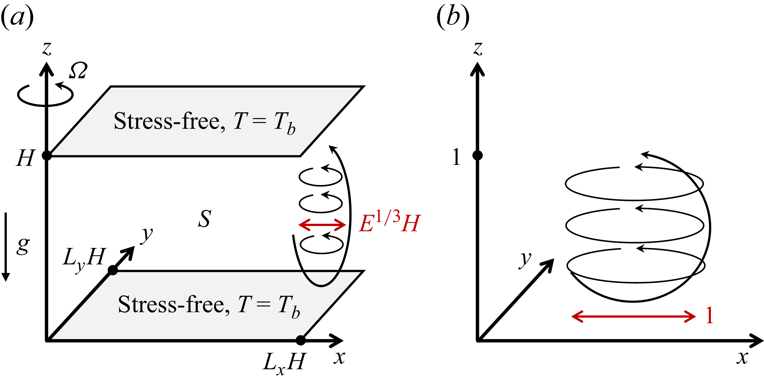
 S
 H
 g
 LxH
 LyH
 Ω
 Tb=0
 H
 E1/3H
 H
 E1/3H
 E≪1
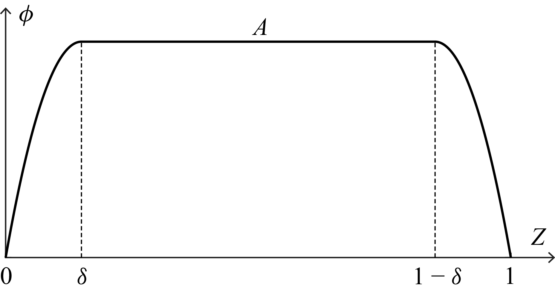
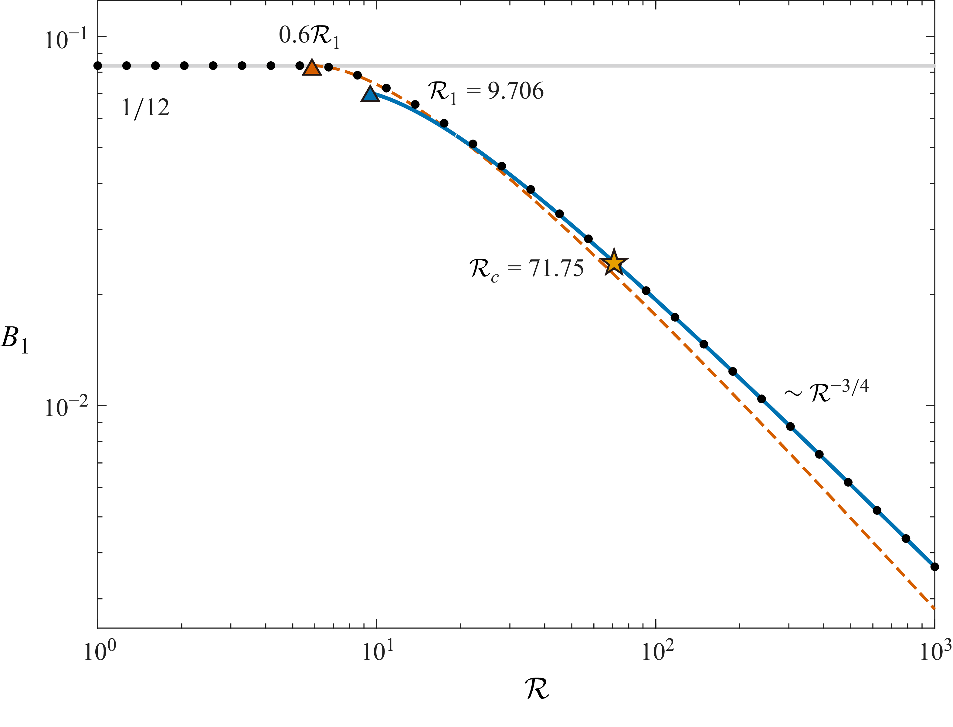
 ⟨Θ⟩V,t
 1/12
 δ≤1/2
 R
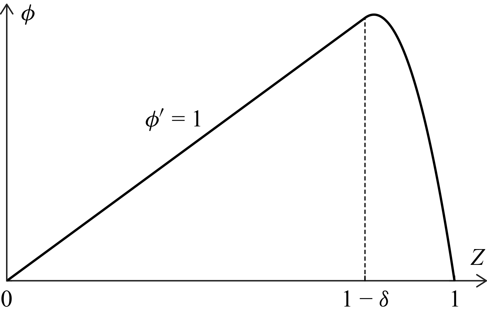
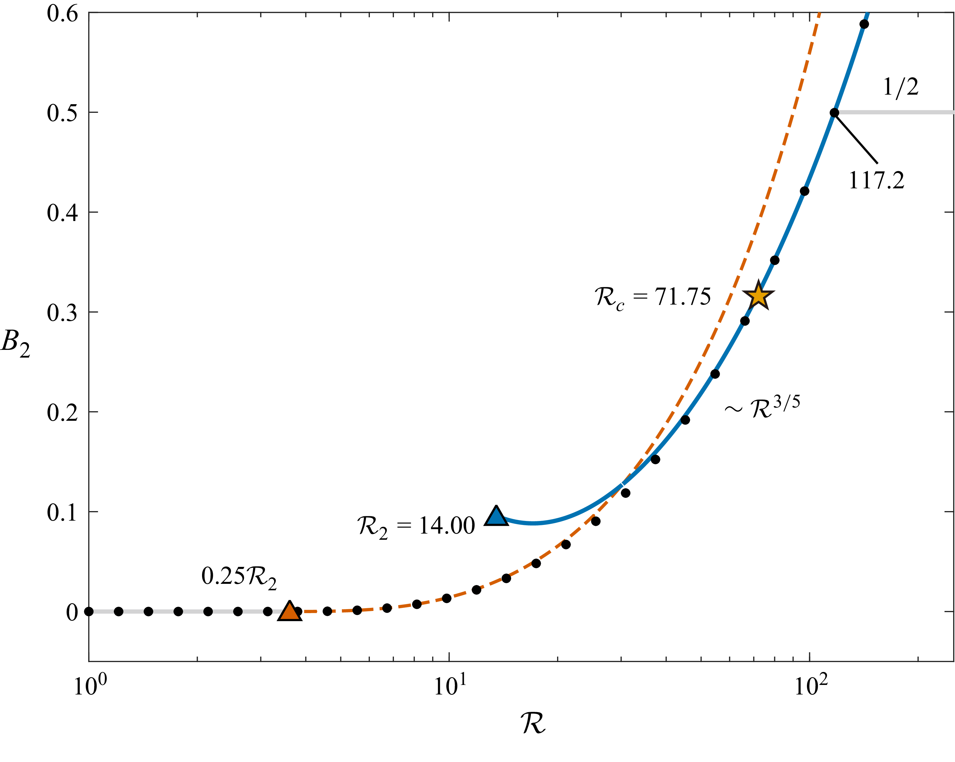
 ⟨wθ⟩V,t
 0
 1/2
 δ≤1
 R

 ⟨Θ⟩V,t
 ⟨wθ⟩V,t
 R
 ϕ(Z)
 ⟨Θ⟩V,t
 1/12
 ⟨Θ⟩V,tR3/4
 R=6.51×10²
 2.47×10³
 8.15×10³
 ⟨wθ⟩V,t
 1/2
 R=300
 500
 1000

 ⟨Θ⟩V,t
 R
 E

 k
 (k,R)
 C1
 C2
 1.867
 5.783×10⁻⁴

 Open access

