2.1 Facility

Table 1.

Typical facility reservoir (subscript 0) and computed free stream (subscript $\infty$ ) properties of the test conditions employed in the experiments of the present study.

All experiments were performed at AEDC Tunnel 9 in White Oak, Maryland. Tunnel 9 is a large-scale hypersonic blowdown tunnel capable of producing a wide range of unit Reynolds numbers and Mach numbers with test durations of up to several seconds. A detailed description of the operational envelope of Tunnel 9 can be found in Lafferty et al. (Reference Lafferty, Coblish, Marineau, Norris, Kurits, Lewis, Smith and Marana2015). In the present study, the Mach number of the flow was approximately 14 over a range of unit Reynolds numbers from 1.74 to $3.62\times 10^{6}~\text{m}^{-1}$ . Nitrogen was used as the test gas. For all conditions the model temperature was nominally room temperature, leading to a wall to stagnation temperature ratio of approximately 0.2. Free stream and reservoir conditions are provided in table 1.

2.2 Model

All experiments were performed on a $7^{\circ }$ -half-angle cone with a nominally sharp nose ( $\text{radius}=0.15~\text{mm}$ ). The length of the cone was $1.55~\text{m}$ . During the steady test time of the tunnel, the model was initially held at zero incidence ( $\pm 0.2^{\circ }$ ) for several hundred milliseconds and then pitched continuously up to $10^{\circ }$ . In the present study, only data captured during the zero incidence period are presented. This reduces the relevant test times to 0.15–0.3 s, depending on the conditions (the shortest test time for the highest unit Reynolds number).

The cone was equipped with a variety of surface sensors placed along multiple streamwise rays emanating from the nosetip. Fast-response pressure measurements were made via PCB model 132-A31 piezoelectric transducers with a frequency range of 11 kHz to 1 MHz. Pressure taps provided mean static measurements of the surface pressure, while temperature-sensitive paint and thermocouples provided heat-transfer measurements from which transition locations were determined. Additional information on the surface-mounted instrumentation can be found in Marineau et al. (Reference Marineau, Moraru and Daniel2017).

2.3 High-speed schlieren visualizations

A conventional Z-type schlieren system was used to produce the visualizations. Illumination was provided via a Cavilux HF pulsed-diode laser that generated pulses of 50 ns duration at 810 nm. Two 30-in diameter, 5-m focal length mirrors collimated the light beam, passed it through the test section, and refocused it on the opposite side. Images were recorded with a Phantom v2512 camera. The camera frame rate was typically set to be slightly above one half of the fundamental frequency of the second-mode disturbances as predicted by the PSE calculations; this was determined to be an adequate tradeoff between having sufficient pixel density in the boundary layer, the total field of view, and capturing the evolution of a wavepacket in time. The number of pixels across the boundary layer thickness ranged from 8 in the highest unit Reynolds number run to 14 in the lowest. In all experiments, approximately 490 mm of the cone’s surface was visible and 1024 pixels were captured across the image span. A knife-edge cutoff set parallel to the facility floor was used to visualize the density gradients approximately normal to the cone’s surface. The behaviour of waves within the boundary layer varied from linear (exponential) growth for condition A to breakdown for condition C (as defined by the appearance of turbulent spots and filling of the power spectra). In figure 1 we show an enhanced image sequence at the highest unit Reynolds number run condition.

A calibration of the schlieren system similar to that outlined in Hargather & Settles (Reference Hargather and Settles2012) was performed to enable quantitative measurements. Calibration was required due to the nonlinear schlieren response of the light rays generated by the circular light source. The calibration object was a circular plano-convex lens with a focal length of 10 m and diameter of 25.4 mm. The incoming collimated light rays are deflected to a degree depending on where they pass through the calibration lens; this in turn causes a pixel-intensity gradient to form across the lens in the schlieren image. This intensity gradient in conjunction with knowledge of the density disturbance field created by the lens allows a unique mapping of pixel intensity to density gradient. Additional details on the calibration process can be found in Kennedy et al. (Reference Kennedy, Laurence, Smith and Marineau2017).

Figure 1.

Contrast enhanced image sequence from condition C showing the propagation and development of a second-mode wavepacket. Every third image in the data set is shown. The top image shows the full schlieren image, including the shock from the cone nosetip; subsequent images are cropped. The markers indicate the approximate extent of the wavepacket in the first image and have been translated downstream in subsequent images using the mean wavepacket propagation speed (see § 3.1).

2.4 Time signal reconstruction

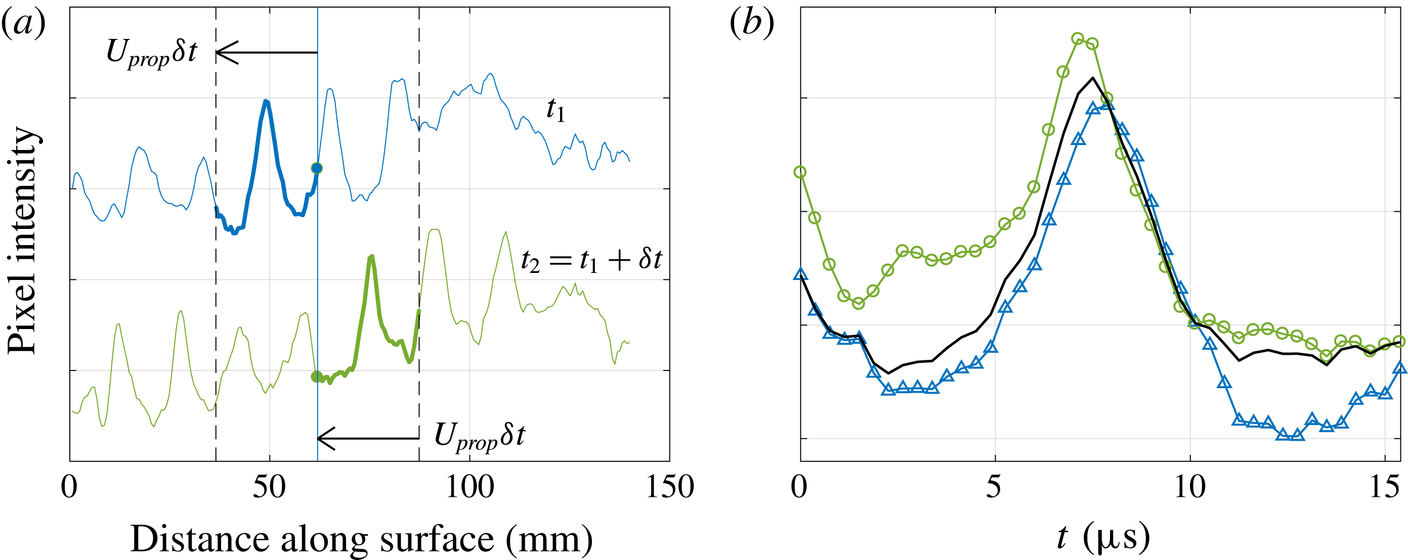
In order to facilitate a time-averaged analysis, time-resolved pixel-intensity signals at specific locations were reconstructed using the spatial data available in the schlieren images. The reconstruction procedure is summarized in figure 2. Consider the pixel intensity at a specific location $(x_{0},y_{0})$ in two consecutive images, at times $t_{1}$ and $t_{2}=t_{1}+\unicode[STIX]{x1D6FF}t$ . The intensity values are known exactly at times $t_{1}$ and $t_{2}$ , but it is desired to reconstruct the intermediate values. If we assume the flow structures to be frozen and propagating horizontally at a speed $U_{prop}$ (for which we will use the average wavepacket propagation speed – see § 3.1), then we have two possibilities available for these intermediate values: the pixel intensities between $x_{0}-U_{prop}\unicode[STIX]{x1D6FF}t$ and $x_{0}$ in the first image, and those between $x_{0}$ and $x_{0}+U_{prop}\unicode[STIX]{x1D6FF}t$ in the second image (figure 2 a). Since the first interval will be more appropriate for times close to $t_{1}$ and the second interval for times close to $t_{2}$ , we take a linearly weighted average of the two, the resulting composite signal matching exactly the known points at $t_{1}$ and $t_{2}$ (figure 2 b). In general, $U_{prop}\unicode[STIX]{x1D6FF}t$ will not correspond to an integer number of pixels, and thus interpolation will be required in generating this composite signal. By repeating for all image pairs of interest, a reconstructed temporal signal is obtained with an effective sampling frequency of $f_{eff}=U_{prop}/\unicode[STIX]{x1D6FF}x$ , where $\unicode[STIX]{x1D6FF}x$ is the visualized distance between neighbouring pixels (in the present case, $f_{eff}\approx 3~\text{MHz}$ ).

The reconstruction was applied to produce time-resolved pixel-intensity signals between streamwise coordinates $s=0.77$ and $1.17~\text{m}$ in increments of $6.2~\text{mm}$ , resulting in 66 unique signals per run. For this work, the signals were reconstructed at the wall-normal location with the largest disturbance amplitude (as identified in an average flow-on image). Interpolation was used to generate the signal at the fixed $y/\unicode[STIX]{x1D6FF}$ location, taking into account the boundary layer height downstream. The thin-lens calibration was then used to convert the pixel intensities to density gradients.

Figure 2.

(a) Schematic showing pixel intensities corresponding to the same segment of a wavepacket at times $t_{1}$ and $t_{1}+\unicode[STIX]{x1D6FF}t$ . Direction of arrow indicates increasing time $t$ . (b) Linear weighting of signals (-▵-, $t_{1}$ signal; -○-, $t_{2}$ signal; ——, weighted signal) to generate reconstructed signal.

3.1 Propagation speeds and frequency spectra

Wavepacket propagation speeds are calculated using the correlation techniques described in Laurence et al. (Reference Laurence, Wagner and Hannemann2016). Because of the enormous number of images gathered per data set, the images are first processed by a feature detection algorithm that identifies the presence and, if applicable, location of a wavepacket (Shumway & Laurence Reference Shumway and Laurence2015). The images are then bandpass filtered around the second-mode fundamental wavelength, and a cross-correlation is applied to image pairs throughout the sequence. Calculated wavepacket propagation speeds are provided in table 2.

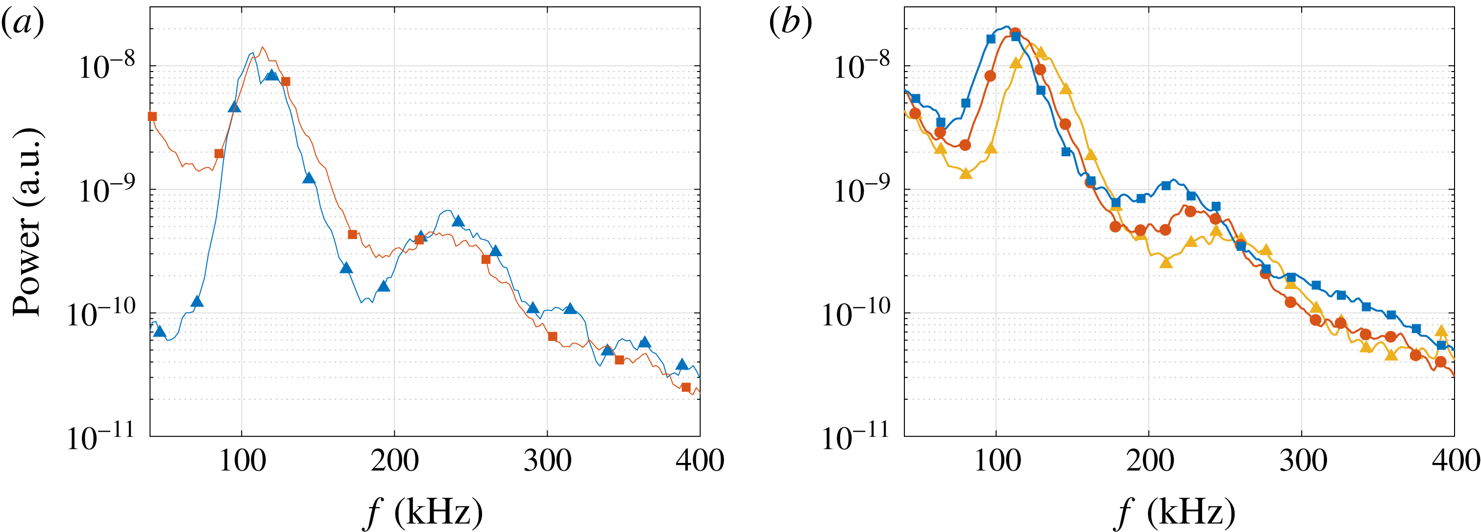
Figure 3(a) shows the power spectral density (PSD) generated from PCB and reconstructed schlieren signals at the same downstream location. Spectra were computed from a signal of $45.8~\text{ms}$ of steady flow using Welch’s method, averaging 100 windows with 50 % overlap. Good agreement is observed in the location and width of the fundamental and first harmonic peaks at approximately 120 and 240 kHz. The power associated with the reconstructed signal at the lower end of the frequency spectrum is significantly larger in the schlieren PSD, likely due to large wavelength structures from the nozzle wall in the visualization path. Figure 3(b) shows the development of the reconstructed frequency spectra with increasing $s$ . As expected, the fundamental and harmonic peaks shift to lower frequencies as the boundary layer grows downstream.

Figure 3.

(a) PSD generated from reconstructed schlieren signal (-▫-) and PCB signal (-▵-) at $s=0.91~\text{m}$ for condition C. (b) PSD generated from schlieren signal at different streamwise locations (condition C: -▵-, $s=0.82~\text{m}$ ; -○-, $s=0.94~\text{m}$ ; -▫-, $s=1.07~\text{m}$ ).

Table 2.

Calculated wavepacket propagation speeds.

3.2 $N$ factors of the most-amplified second-mode frequencies

Using the PSD curves computed from the reconstructed density-gradient signals, the $N$ factors are computed as

(3.1) $$\begin{eqnarray}N(f,s_{i})=\frac{1}{2}\ln \left(\frac{\text{PSD}(f,s_{i})}{\text{PSD}(f_{1},s_{1})}\right),\end{eqnarray}$$

where $\text{PSD}(f,s_{i})$ is defined as the peak power of frequency $f_{0}$ at streamwise location $s_{i}$ , and $f_{1}$ is the most-amplified second-mode frequency at the first upstream measurement location, $s_{1}$ . Based on estimates of the change in initial disturbance amplitude with frequency, the initial disturbance amplitudes are assumed equal over the fairly narrow range of $f_{0}$ for each run. Comparison of growth rates between two downstream locations is made possible by assuming the change in boundary layer height is negligible between the measurement locations. Applying this assumption, the ratios of the density and density-gradient disturbance amplitudes are equal, i.e., $\unicode[STIX]{x1D70C}^{\prime }(s_{2})/\unicode[STIX]{x1D70C}^{\prime }(s_{1})=\unicode[STIX]{x1D70C}_{y}^{\prime }(s_{2})/\unicode[STIX]{x1D70C}_{y}^{\prime }(s_{1})$ , where prime denotes disturbance and subscript $y$ denotes the derivative with respect to $y$ . 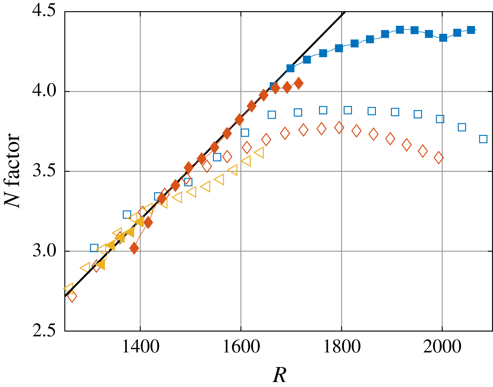The $N$ factors calculated from the schlieren signals, PCB measurements and PSE solutions are plotted versus stability Reynolds number ( $R$ ) in figure 4. Here, we define the stability Reynolds number based on the free stream conditions and surface coordinate ( $R=\sqrt{Re_{s}}$ ), as Marineau et al. (Reference Marineau, Moraru and Daniel2017) previously used this definition to successfully scale second-mode growth rates on a sharp cone at Mach 14. The PSE results were computed using the PSE-Chem solver of the STABL software suite (Johnson & Candler Reference Johnson and Candler2005). PSE-Chem solves the two-dimensional, axisymmetric, linear parabolized stability equations to predict the amplification of disturbances within the boundary layer. The disturbance growth rate is calculated from the total kinetic energy of the disturbance and has been shown to be equal to the growth rate calculated from other flow variables (Chang, Vinh & Malik Reference Chang, Vinh and Malik1997). A fit of maximum $N$ factor versus stability Reynolds number generated from the PSE solutions is presented in figure 4. Additional information on the PSE calculations can be found in Marineau et al. (Reference Marineau, Moraru and Daniel2017). We note that since the second-mode waves were already developed at the most upstream viewing location, the initial values of the $N$ factors calculated from the schlieren signals are arbitrary. To account for this, the schlieren $N$ factors are vertically shifted to overlay the PSE curve. In general, the slopes of the PSE, PCB and schlieren curves agree well until saturation is reached. Maximum $N$ factors calculated from the schlieren signals saturate at larger $R$ values than their PCB counterparts, resulting in greater absolute $N$ factors (good agreement is seen for the regions of linear growth at lower unit Reynolds numbers). Only the most downstream locations are included for condition A as the upstream second-mode waves were too weak to provide an adequate signal.

Figure 4.

$N$ factors calculated for the most-amplified second-mode frequencies at different conditions (- ${\vartriangleleft}$ -, condition A; - $\diamondsuit$ -, condition B; - $\Box$ -, condition C; —, PSE solution). Filled markers indicate schlieren measurements; open markers indicate PCB measurements.

3.3 Streamwise development of $N$ factors

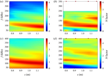
Figure 5 shows the development of the second-mode disturbances as a function of streamwise location. Here, schlieren signals have been used to calculate the $N$ factors for distinct frequencies at each streamwise location. The $N$ factors generated from the PCB sensor data are calculated similarly with interpolation between the (rather sparse) sensor locations.

In figure 5(a,b), for condition B, the $N$ factors calculated from the schlieren signals match well with those calculated from the PCB signals in the linear growth region. The fundamental frequency band broadens for the schlieren $N$ factors with increasing streamwise distance. Growth of the first harmonic occurs in the same frequency range in both the schlieren and PCB measurements. At any given streamwise location, the ratio between the $N$ factors at $f_{0}$ and the first harmonic tends to be larger for the schlieren signal (i.e. the harmonic is relatively weaker).

Figure 5.

$N$ factors as a function of streamwise location: (a,b) Condition B, (c,d) condition C; (a,c) calculated from schlieren visualizations; (b,d) calculated from PCB measurements. Data above 250 kHz are omitted from (b) due to noise in the PCB sensors. Red dots indicate streamwise locations of PCB sensors.

In figure 5(c,d) we show the streamwise development of the $N$ factors at the highest unit Reynolds number condition C. A clear discrepancy exists between the development of the schlieren and PCB $N$ factors. The disturbance at $f_{0}$ saturates at approximately $s=0.8~\text{m}$ in the PCB measurements, while saturation in the schlieren measurements occurs between $s=1.1$ and $1.2~\text{m}$ (also seen in figure 4). Similar behaviour is seen for the first harmonic. The measured frequencies of both the fundamental disturbance and the first harmonic agree well between the two measurement techniques. The difference in $N$ factor saturation location may be linked to several causes. First, nonlinear growth close to saturation may not be uniform across the boundary layer thickness, causing the PCB measurements made at the surface of the cone to differ from the schlieren measurements made off the model’s surface. The integration effect inherent to the schlieren system may also play a role; as the breakdown process begins and features become increasingly three-dimensional, the schlieren signal will become unable to resolve them accurately. The assumption of negligible change in boundary layer height may begin to break down in this region as well. Finally, the PCB sensors record pressure fluctuations while the schlieren signals measure density gradients, two measurements whose relationship is not clearly defined in the nonlinear growth region. Further investigations will address the source of this discrepancy.

3.4 Bispectral analysis

In the $N$ factor plots presented in § 3.3, we noted the presence of harmonics. The presence of these harmonics motivates the search for nonlinear interactions. By calculating a bicoherence for the density-gradient signals, nonlinear phase-coupled quadratic interactions of waves can be identified and distinguished from spontaneous excitation (see Chokani Reference Chokani2005, Hofferth et al. Reference Hofferth, Humble, Floryan and Saric2013). We define the bicoherence as

(3.2) $$\begin{eqnarray}b^{2}(f_{1},f_{2})=\frac{|E[X(f_{1})X(f_{2})X^{\ast }(f_{1}+f_{2})]|^{2}}{E[|X(f_{1})X(f_{2})|^{2}]E[|X(f_{1}+f_{2})|^{2}]},\end{eqnarray}$$

where $E$ is the expectation operator, $X(f)$ is the Fourier transform of a segment of the time series record, and $^{\ast }$ indicates the complex conjugate. The $b^{2}$ value is bounded by 0 and 1, these two extremes indicating no phase coupling (spontaneous excitation) and complete phase locking, respectively. In practice, noise in experimentally obtained signals reduces the upper bicoherence to a value less than 1 (Kimmel & Kendall Reference Kimmel and Kendall1991).

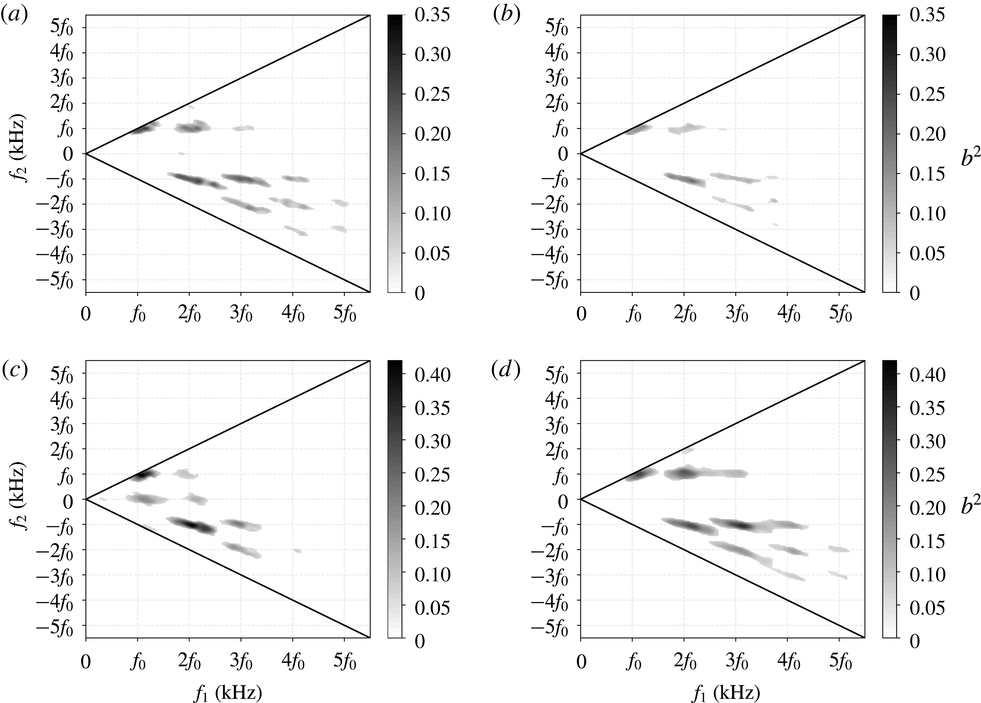
In figure 6 we show the bicoherence calculated from time-resolved density-gradient signals at two streamwise locations for conditions B and C (no nonlinear interactions were present for condition A). The bicoherence values were calculated using Hann windows 256 points in length with 50 % overlap. Focusing first on (higher unit Reynolds number) condition C, at the upstream measurement location ( $s=0.81~\text{m}$ ), a strong sum interaction exists at $f_{0}+f_{0}\rightarrow 2f_{0}$ and 2 $f_{0}+f_{0}\rightarrow 3f_{0}$ , indicating disturbances at $f_{0}$ coupling to generate a harmonic at $2f_{0}$ , and interaction of the harmonic content at $2f_{0}$ with disturbances at $f_{0}$ to generate a second harmonic at $3f_{0}$ . A weak interaction also exists at $3f_{0}+f_{0}\rightarrow 4f_{0}$ and $2f_{0}+2f_{0}\rightarrow 4f_{0}$ indicating slight amplification of a third harmonic. Difference interactions (lower-right quadrant) are also present between each of the higher harmonics. In general, bicoherence was maximum at the most upstream measurement location for this condition with peak values of 0.25–0.3 and decreased continuously downstream. For example, at $s=0.88~\text{m}$ (figure 6 b) bicoherence values for all interactions have decreased compared to $s=0.81~\text{m}$ , and interactions involving a third harmonic have disappeared. No significant quadratic coupling is present by $s=1.15~\text{m}$ (not shown) where growth of the disturbances has saturated and the boundary layer is on the verge of breaking down; at this point the interactions are either no longer quadratic or the remaining fluctuations are random.

We now turn our attention to condition B (figure 6 c,d). At the upstream location ( $s=0.78~\text{m}$ ) strong sum and difference interactions are seen between higher harmonics up to $3f_{0}$ . Additionally, interactions exist at $f_{0}+0\rightarrow f_{0}$ and $2f_{0}+0\rightarrow 2f_{0}$ indicating that the power spectrum is being filled. The bicoherence reaches a peak value of 0.37–0.41 in the $f_{0}+f_{0}\rightarrow 2f_{0}$ interaction and remains at this level until decreasing at approximately $s=1.09~\text{m}$ . Further downstream ( $s=1.14~\text{m}$ , figure 6 d), additional interactions are present, including sum and difference interactions between third and fourth harmonics. The contours have also broadened in bifrequency space, indicating that the fundamental frequency disturbance and its harmonics are coupling with their sidebands.

By examining the bicoherence plots shown in figure 6 in conjunction with the $N$ factors shown in figures 4 and 5, we see that strong nonlinear interactions are present when the fundamental disturbance is still being amplified within the linear region. The strength of the nonlinear interaction generating the first harmonic appears to be more closely linked to the amplification rate (the slope of the $N$ factor curves) of the first harmonic rather than the $N$ factor of the first harmonic. For condition B, the first harmonic is strongly amplified from the most upstream location until approximately $s=1.05~\text{m}$ when the amplification rate decreases; this decrease in amplification rate coincides with a decrease in bicoherence values. For condition C, the $N$ factor of the first harmonic increases over the entire measurement range, while both the amplification rate of the first harmonic and the bicoherence value describing that interaction are decreasing. We also note that for condition C, the first harmonic reaches a maximum $N$ factor at a streamwise location where no significant nonlinear interactions are present. In addition, nonlinear interactions involving higher harmonics ( $3f_{0}$ , $4f_{0}$ , $5f_{0}$ ) appear in the bicoherence plots while having little to no power in the PSD plots.

Figure 6.

Bicoherence $b^{2}$ values calculated for condition C (a,b) and condition B (c,d) at locations: (a)  $s=0.81~\text{m}$ , $R=1705$ ; (b)  $s=0.88~\text{m}$ , $R=1782$ ; (c)  $s=0.78~\text{m}$ , $R=1399$ ; (d)  $s=1.14~\text{m}$ , $R=1692$ . Black lines indicate planes of symmetry. The frequencies are represented by the fundamental disturbance frequency at the given streamwise location.