1 Introduction
Airflow over water waves represents a challenging problem relevant both in nature and for engineering applications, such as stratified two-phase pipe flows, which are the focus of this work. Considering wind over waves, two of the most characteristic features for the liquid and gas phases, respectively, is wave breaking and airflow separation. Wave breaking occurs when fluid elements at the surface overtake the general waveform, resulting in increased turbulence in the liquid phase and a transfer of momentum and energy from the waves to the underlying flow (Banner & Melville Reference Banner and Melville1976; Jessup, Zappa & Yeh Reference Jessup, Zappa and Yeh1997). Airflow separation over surface waves is characterized by increased turbulence in the air phase as the shear layer separates from the interface, and a significant displacement of the streamlines relative to the wave shape. This results in a distribution of pressure and shear forces along the wave profile which deviate significantly from the non-separated case (Weissman Reference Weissman1986). Analysis of these phenomena in the pipe flow literature are scarce, hence we refer to the air–sea literature for a background to the understanding of wave breaking and airflow separation.
Banner & Melville (Reference Banner and Melville1976) and Gent & Taylor (Reference Gent and Taylor1977) considered separation above water waves as ‘the occurrence, in a frame of reference moving with the waves, of a streamline leaving the water surface’. This requires the surface velocity of the interface to match the wave speed, which is the criterion for incipient wave breaking. Hence, it was concluded that airflow separation may only occur in conjunction with wave breaking. This criterion has been applied by researchers modelling drag on the sea surface (Kudryavtsev & Makin Reference Kudryavtsev and Makin2001). However, early flow visualization techniques indicated that airflow patterns resembling the separated flow over solid obstacles may occur over non-breaking waves (Kawai Reference Kawai1981, Reference Kawai1982; Weissman Reference Weissman1986). According to Weissman (Reference Weissman1986), the separation criterion utilized by Banner & Melville (Reference Banner and Melville1976) and Gent & Taylor (Reference Gent and Taylor1977) is not appropriate when the surface is moving, as airflow separation over moving boundaries may have stagnation points away from the wall. As described by Weissman (Reference Weissman1986); ‘the “separation” we are concerned with is that of the shear layer closest to the surface…’. Buckley & Veron (Reference Buckley and Veron2016) considered the airflow as separating ‘if the near-surface, high vorticity layer characteristic of an attached boundary layer is ejected away from the water surface and the surface vorticity is near zero or negative’. A similar criterion was also applied by Reul, Branger & Giovanangeli (Reference Reul, Branger and Giovanangeli2008) and Sullivan et al. (Reference Sullivan, Banner, Morison and Peirson2018b ).
Applying the definition of (shear layer) separation by Weissman (Reference Weissman1986), Reul et al. (Reference Reul, Branger and Giovanangeli2008) and Buckley & Veron (Reference Buckley and Veron2016), it has been documented both experimentally (Veron, Saxena & Misra Reference Veron, Saxena and Misra2007; Tian, Perlin & Choi Reference Tian, Perlin and Choi2010) and numerically (Sullivan et al. Reference Sullivan, Banner, Morison and Peirson2018b ) that separation may occur over non-breaking waves. Wave breaking has been found to be a sufficient, but not a necessary, condition for airflow separation (Tian et al. Reference Tian, Perlin and Choi2010; Sullivan et al. Reference Sullivan, Banner, Morison and Peirson2018b ).
Wave breaking is separated into categories related to the severity and visual characteristics of the breaking process. Babanin (Reference Babanin2011) divides wave breaking into plunging, spilling and microbreaking. Microbreaking, or microscale breaking, is a weak form of wave breaking, where surface tension prevents the jet formation and air entrainment into the liquid phase as the wave breaks (Jessup et al. Reference Jessup, Zappa and Yeh1997; Tulin & Landrini Reference Tulin and Landrini2001; Siddiqui & Loewen Reference Siddiqui and Loewen2006; Vollestad, Ayati & Jensen Reference Vollestad, Ayati and Jensen2019b ). Microscale breaking waves are short (wavelength of the order of a few decimetres), wind generated waves with amplitudes up to a few centimetres. In the present work we focus our attention on these small scale breaking waves.
We consider stratified wavy two-phase pipe flow. These flows have traditionally been modelled using a simple two-fluid model, which in addition to a modified single-phase correlation for the wall friction, relies on a parametrization of the interface friction factor (Ullmann & Brauner Reference Ullmann and Brauner2006). The interfacial friction factor has typically been established through correlation studies based on pressure drop and liquid hold-up measurements (see e.g. Tzotzi & Andritsos Reference Tzotzi and Andritsos2013), yielding little physical insight into the mechanisms that govern the momentum exchange at the interface. Recently, stratified gas–liquid pipe flow has been analysed using particle image velocimetry (PIV) in the centreplane of the gas and liquid phase (Ayati et al.
Reference Ayati, Kolaas, Jensen and Johnson2014, Reference Ayati, Kolaas, Jensen and Johnson2016; Birvalski et al.
Reference Birvalski, Tummers, Delfos and Henkes2015; Birvalski, Tummers & Henkes Reference Birvalski, Tummers and Henkes2016). These studies have provided spatio-temporally and phase-averaged flow fields, and hence valuable experimental data for model validation of more complex numerical models, and new insight into the dynamics of the two phases. Previous analysis of the experimental set-up considered in this work (Vollestad et al.
Reference Vollestad, Ayati, Angheluta, LaCasce and Jensen2019a
) has shown that intermittent airflow separation is a frequent event as the gas flow rate in increased into the amplitude saturation regime described by Ayati et al. (Reference Ayati, Kolaas, Jensen and Johnson2015), and microscale wave breaking has been observed when the superficial gas velocity
 $U_{sg}\geqslant 1.8~\text{m}~\text{s}^{-1}$
, for a superficial liquid velocity
 $U_{sl}=0.1~\text{m}~\text{s}^{-1}$
(Vollestad et al.
Reference Vollestad, Ayati and Jensen2019b
) (the superficial velocity of phase
 $k$
is
 $U_{sk}={\dot{m}}_{k}/(\unicode[STIX]{x1D70C}_{k}A)$
, where
 ${\dot{m}}_{k}$
and
 $\unicode[STIX]{x1D70C}_{k}$
are the mass flow rate and density of phase
 $k$
, while
 $A$
is the cross-sectional area of the pipe). Microscale wave breaking was found to influence the liquid phase down to a depth of approximately 1 cm below the crest (approximately one significant wave height), increasing the turbulent dissipation rate below the crest by a factor 3–4 compared with non-breaking waves (Vollestad et al.
Reference Vollestad, Ayati and Jensen2019b
). These results are consistent with observations of microscale breaking waves in wind–wave tanks (Siddiqui & Loewen Reference Siddiqui and Loewen2007, Reference Siddiqui and Loewen2010), indicating that the main features of microscale breaking waves in two-phase pipe flow are similar to the processes occurring in the ocean.
When small scale wind waves go from incipient to active breaking, a thin spilling region is generated on the leeward side of the wave crest, resulting in increased turbulence and vorticity in the liquid phase. The present understanding of how active breaking influences the airflow field above waves and airflow separation is however far from complete (Sullivan et al. Reference Sullivan, Banner, Morison and Peirson2018b ). While previous analysis of two-phase pipe flow has documented that both airflow separation and microscale wave breaking occurs for sufficiently high gas flow rates, the link between the two has not previously been investigated in a pipe flow set-up.
Analysing airflow over waves by PIV in a rectangular wind–wave tank, Reul et al. (Reference Reul, Branger and Giovanangeli2008) found that the separation induced by breaking waves is stronger and more consistent than separation over non-breaking waves. Reul et al. (Reference Reul, Branger and Giovanangeli2008) performed measurements over waves ranging from microbreaking to plunging, the claim is not specific for microscale breaking waves. Banner (Reference Banner1990) evaluated the pressure and velocity field over small scale incipient and actively breaking waves, using a slope exceedance threshold to distinguish between breaking and non-breaking waves. Banner (Reference Banner1990) reports that while there is a significant phase shift of the pressure field also for unbroken steep waves, active wave breaking results in an increased (order 100 %) phase shift and form drag above the wave profiles. Similar results were found by numerical analysis by Maat & Makin (Reference Maat and Makin1992), who concluded that the increased local roughness in the spilling region enhanced the asymmetrical surface pressure pattern. Recently, Sullivan et al. (Reference Sullivan, Banner, Morison and Peirson2018b
) performed large eddy simulations (LES) of airflow above wave profiles taken from the experiments of Banner (Reference Banner1990). Example wave profiles of incipient and actively breaking waves (
 $ak=0.25$
, 0.28,
 $c/u_{\ast }=1.58$
, 1.23 for incipient and active breaking respectively) were investigated. Based on parameter tuning of the numerical model, they found that the wave steepness, not the enhanced surface drift caused by wave breaking, was the critical property inducing large form drag over the actively breaking waves, indicating that the geometrical properties of the waves (and not the state of wave breaking) dictates the surface drag. Recent two-fluid direct numerical simulations (DNS) by Yang, Deng & Shen (Reference Yang, Deng and Shen2018) have shown that, while a plunging breaker will significantly impact the airflow field, a spilling breaker (initial steepness
 $ak=0.35$
) under relatively strong wind forcing (
 $c/u_{\ast }=3.7$
) does not significantly influence the airflow as the wave transitions from a smooth unbroken wave form to a spilling breaker. Simulations by Yang et al. (Reference Yang, Deng and Shen2018) indicate that the form drag remains essentially constant as the wave evolves into an active spilling breaker.
In this work we perform simultaneous two-phase PIV, to obtain two-dimensional (2-D) velocity fields in both the gas and liquid phases. The technique was first applied by Ayati et al. (Reference Ayati, Kolaas, Jensen and Johnson2014) for two-phase pipe flow. The novelty of this work lies in the simultaneous assessment of active wave breaking and evaluation of the airflow above individual waves. Wave breaking is assessed by the method of Vollestad et al. (Reference Vollestad, Ayati and Jensen2019b ), evaluating the root-mean-square (r.m.s.) vorticity in the liquid phase on the leeward side of the crest. Statistics of the flow field over breaking and non-breaking waves at two different gas flow rates are examined. The goal is to investigate how active wave breaking affects the airflow above waves compared with non-breaking waves of similar steepness. Understanding the effect of small scale wave breaking and its link to airflow separation in stratified two-phase pipe flow is assessed to be an important step in quantifying the physical processes responsible for the momentum exchange at the interface between the two phases. While the closed pipe geometry impacts the flow, making a direct comparison with the processes occurring in the ocean inaccurate, the results obtained in the present work may also provide insight into the processes occurring in an open system, as the underlying mechanisms (wave breaking and airflow separation) are the same. The simultaneous assessment of active wave breaking and airflow separation above microscale breaking waves has, to the authors’ knowledge, not previously been documented for either an open or closed air–water system.
This paper is organized in six sections (including this introduction). In § 2 the experimental set-up is presented. In § 3 the experimental cases and methodology are presented. Results are presented in § 4. Instantaneous flow fields are presented in § 4.1, while the statistics of the airflow field above breaking and non-breaking waves are presented in § 4.2. A detailed analysis of waves within a narrow steepness band is performed in § 4.3. Finally, a discussion and concluding remarks are presented in §§ 5 and 6.
2 Experimental set-up
The experiments were conducted at the Hydrodynamics Laboratory at the University of Oslo. The experimental set-up consists of a 31 m long, horizontal, transparent, acrylic pipe with an internal diameter
 $D=10~\text{cm}$
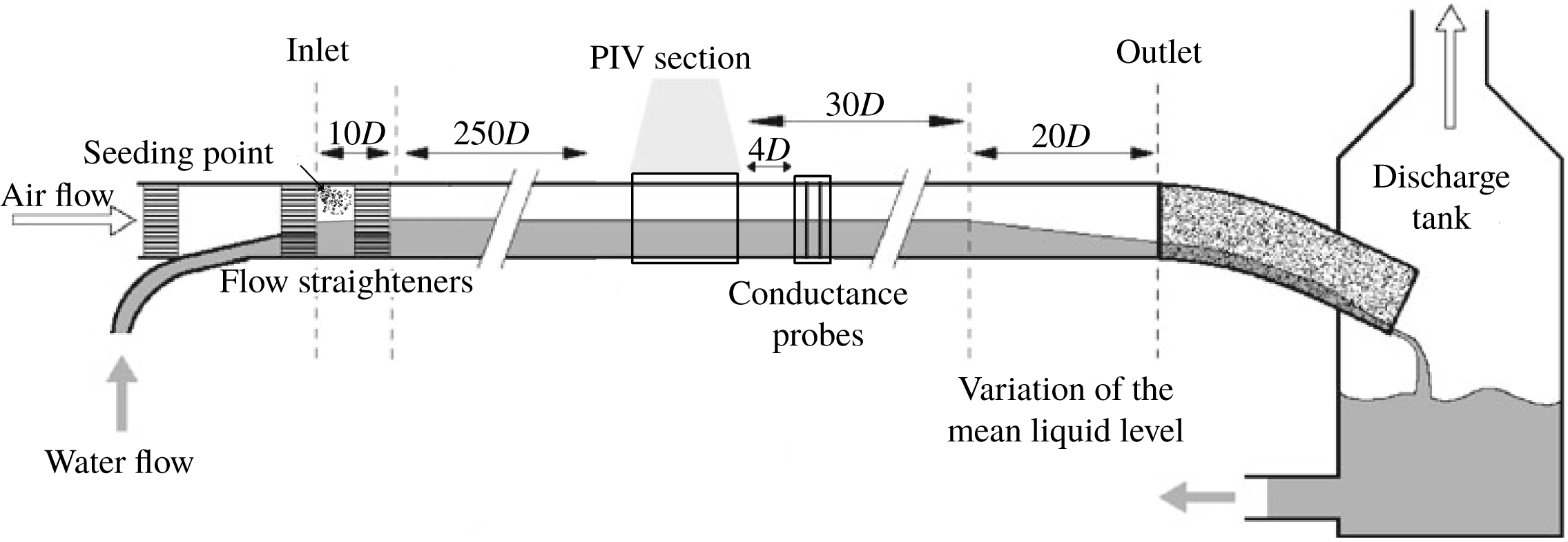
. An overview of the experimental set-up is presented in figure 1. Air and water were supplied at the inlet by a frequency regulated fan and pump respectively. Here, honeycomb flow straighteners were placed to dampen turbulent fluctuations introduced at the inlet. The gas and liquid flow rates were measured using an Emerson MicroMotion Coriolis flow meter and an Endress Hauser Promass Coriolis flow meter respectively. At the pipe outlet the fluids were discharged to a tank (at atmospheric pressure), and recirculated. The differential pressure in the air phase was measured over a 12.4 m section, using a smar LD301 differential pressure gauge.
Schematic view of experimental set-up.

A PIV section was placed 260
 $D$
from the pipe inlet. Here, an optical correction box was placed around the pipe. The box was half-filled with water to reduce optical distortion of the liquid-phase PIV camera. A nonlinear coordinate transform was obtained for each of the cameras applied by imaging a coordinate system placed in the pipe centreline, using the coordinate system described in Ayati et al. (Reference Ayati, Kolaas, Jensen and Johnson2015). PIV was conducted simultaneously in the centreplane of both phases. A 147 mJ ND:YAG laser (532 nm wavelength light) illuminated the centreplane of the PIV section from above. The head of the laser optics was placed 50 cm above the pipe centreline, creating a thin (
 ${<}1$
mm) laser sheet within the measurement section.
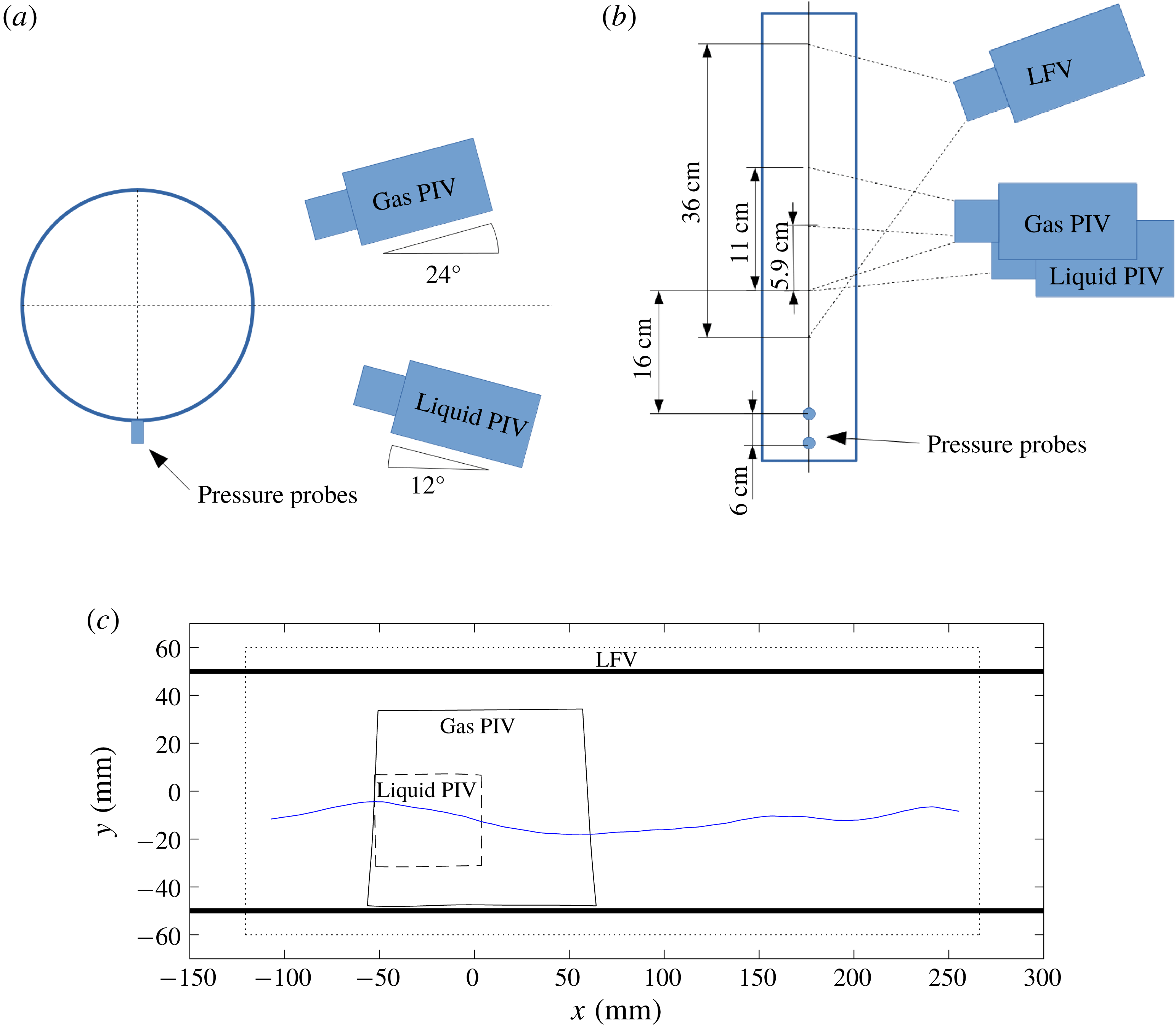
Three cameras were employed in the study. Their position and field of view (FOV) are shown in figure 2.
(1) Liquid-phase PIV camera. PCO.4000 camera with
 $4008\times 2672$
pixels. Fitted with a 100 mm lens and a
$1.6\times$
teleconverter. The camera is directed upwards at an angle of
$12^{\circ }$
.
(2) Gas-phase PIV camera. PCO.4000 camera with
$4008\times 2672$
pixels. Fitted with a 100 mm lens. The camera is directed downwards at an angle of
$24^{\circ }$
. A high downwards looking angle was necessary as the crescent shape of the waves meant that the pipe wall was repeatedly wetted well above the mean water level.(3) Large field of view (LFV) camera. A Nikon D7200 with
$6400\times 4000$
pixels. Fitted with a 28 mm lens. The camera was directed downwards at an angle of
$30^{\circ }$
, and looking upstream at an angle of approximately
$31^{\circ }$
.


Schematic view of PIV measurement section. (a) Looking downstream. (b) Seen from above. (c) FOV of all three cameras. Blue line represents an example interface profile (waves propagating to the right).

Due to the relatively high downward/upwards looking angle of the gas/liquid phase PIV cameras, these were fitted with Scheimpflug adapters, allowing the entire centreplane of the pipe to be in focus.
The gas phase was seeded with small water particles, generated by a high-pressure atomizer. The particles were injected into the gas phase at the inlet. According to the manufacturer, 72 % of the droplets are below
 $6~\unicode[STIX]{x03BC}\text{m}$
, and it has previously been shown by Ayati et al. (Reference Ayati, Kolaas, Jensen and Johnson2014) that the particles exhibit a Stokes number well below 1 for the flow rates of interest.
Initial analysis using polyamide particles in the liquid phase showed that light reflections from particles near the spilling region of microscale breaking waves influenced the gas-phase PIV images, causing unreliable results near the gas–liquid interface. This issue was overcome by using fluorescent particles in the liquid phase and fitting the gas-phase PIV camera with a bandpass filter centred at 532 nm (midopt BP525 Light Green Bandpass Filter). The liquid phase was seeded with fluorescent particles made from a commercially available acrylic paint (Lefranc & Bourgeois, Fluorescent light orange). Particles made from this paint were used also by Birvalski et al. (Reference Birvalski, Tummers, Delfos and Henkes2015) to perform PIV in the liquid phase of two-phase pipe flow. The particles were extracted in a settling process, similar to the process described by Birvalski (Reference Birvalski2015). Visual inspection of the particles under the microscope revealed that the particle size typically ranged from 5 to
 $20~\unicode[STIX]{x03BC}\text{m}$
.
For efficient interface detection, Rhodamine B was added to the water at a concentration of
 $5\times 10^{-5}~\text{g}~\text{l}^{-1}$
. A filter closely matching the wavelength emitted from the rhodamine (B+W 041 red/orange filter) was added to the LFV camera. This removed the green signal from the droplets in the air phase, allowing for efficient interface detection from the LFV camera. The interface was detected by a thresholding technique, similar to the technique applied by Vollestad et al. (Reference Vollestad, Ayati and Jensen2019b
), and transferred to the gas- and liquid-phase PIV images by applying a cubic coordinate transform. By looking through many PIV images (gas and liquid), overlaid the detected interface, the accuracy of the interface detection and coordinate transform is assessed to be approximately 0.4 mm, similar to the PIV resolution.
Two pressure probes (Kulite XTL-190) were mounted flush to the pipe bottom (position indicated in figure 2). The probes measured the pressure at a frequency of 2000 Hz. The pressure was normalized by a normalization filter (output centred at 0 with standard deviation 1) based on the previous 30 s of data sampling. When a pressure peak (associated with a wave crest) above a threshold
 $\unicode[STIX]{x1D70E}$
was detected by the downstream pressure probe, a cross-correlation of the previous one second of data was performed between the two probes, to estimate the wave speed. This estimate was used to evaluate a trigger delay to the PIV system, allowing the leeward side of the wave to be repeatedly present within the liquid phase PIV FOV as the PIV images were acquired (necessary for the analysis performed in this work). The pressure probe trigger system is described in more detail in Vollestad et al. (Reference Vollestad, Ayati and Jensen2019b
).
The two laser pulses were triggered with a
 $\unicode[STIX]{x0394}t$
of
 $100{-}120~\unicode[STIX]{x03BC}\text{s}$
(depending on the flow rate combinations applied). Note that while the PIV cameras acquired double images (one image per laser pulse), the LFV camera was set to trigger before the first laser pulse, and had an exposure time which was longer than the laser pulse
 $\unicode[STIX]{x0394}t$
, i.e. the LFV image was double exposed. During the laser
 $\unicode[STIX]{x0394}t$
, the waves would move less than 0.1 mm, which is a negligible fraction of the overall wave shape, and less than the accuracy of the interface detection.
A conductance wave gauge was placed 4
 $D$
downstream of the PIV section, measuring the interface elevation at 500 Hz. This consists of two double-wire probes of 0.3 mm diameter separated by 4 mm. The two probes were placed in the centre of the pipe with a distance 6 cm in the streamwise direction. For more details on the wave gauges the reader is referred to Ayati et al. (Reference Ayati, Kolaas, Jensen and Johnson2015).
PIV was performed with a cascade of sub-pixel passes, with a final interrogation window of
 $52\times 26$
pixels in the gas phase, and
 $32\times 32$
pixels in the liquid phase, using 50 % overlap. This translates to a spatial resolution of
 $0.75\times 0.38~\text{mm}^{2}$
in the gas phase, and
 $0.24\times 0.24~\text{mm}^{2}$
in the liquid phase. Spurious vectors were detected by standard methods based on a local median filtering (Raffel et al.
Reference Raffel, Willert, Scarano, Kähler, Wereley and Kompenhans2018), and replaced by cubic interpolation.
3 Methodology
3.1 Description of experimental cases
We consider two experimental cases, where the liquid superficial velocity is kept constant at
 $U_{sl}=0.1~\text{m}~\text{s}^{-1}$
, while the gas superficial velocity (
 $U_{sg}$
) is increased from
 $1.85~\text{m}~\text{s}^{-1}$
to
 $2.20~\text{m}~\text{s}^{-1}$
. These experimental cases were chosen as they appear in two different regimes in the flow map. As shown by Vollestad et al. (Reference Vollestad, Ayati and Jensen2019b
), for this liquid flow rate the first interfacial waves are observed at
 $U_{sg}=1.3~\text{m}~\text{s}^{-1}$
.
 $\unicode[STIX]{x1D702}_{rms}$
(the r.m.s. of the interface elevation fluctuations) at the measurement section is observed to increase with
 $U_{sg}$
until
 $U_{sg}\approx 2.0~\text{m}~\text{s}^{-1}$
. At this gas superficial velocity a regime of ‘amplitude saturation’ is observed, and the main characteristics of the wave field are relatively independent of the gas flow rate. This implies that an equilibrium between increased wind input and dissipation is reached, which is reminiscent of the equilibrium range of the ocean wave spectrum (Phillips Reference Phillips1958, Reference Phillips1985). Vollestad et al. (Reference Vollestad, Ayati and Jensen2019b
) found that the first evidence of wave breaking was observed at
 $U_{sg}=1.8~\text{m}~\text{s}^{-1}$
. Increasing the gas velocity into the amplitude saturation regime was observed to increase both the frequency and intensity of the wave breaking events. Hence, for both experimental cases considered, we expect to observe both breaking and non-breaking waves at the measurement section.
In order to observe a reasonable number of both breaking and non-breaking waves (needed to obtain reliable statistics) the lowest
 $U_{sg}$
is set to
 $1.85~\text{m}~\text{s}^{-1}$
rather than
 $1.8~\text{m}~\text{s}^{-1}$
. The trigger threshold
 $\unicode[STIX]{x1D70E}$
was set to 1.6 for the
 $U_{sg}=1.85~\text{m}~\text{s}^{-1}$
case and 1.4 for the
 $U_{sg}=2.20~\text{m}~\text{s}^{-1}$
case. The trigger threshold results in a bias for detecting larger amplitude waves in the system, as the smaller waves will not trigger the PIV system. Setting a higher trigger threshold for the
 $U_{sg}=1.85~\text{m}~\text{s}^{-1}$
case was necessary to observe a reasonable fraction of both breaking and non-breaking waves.
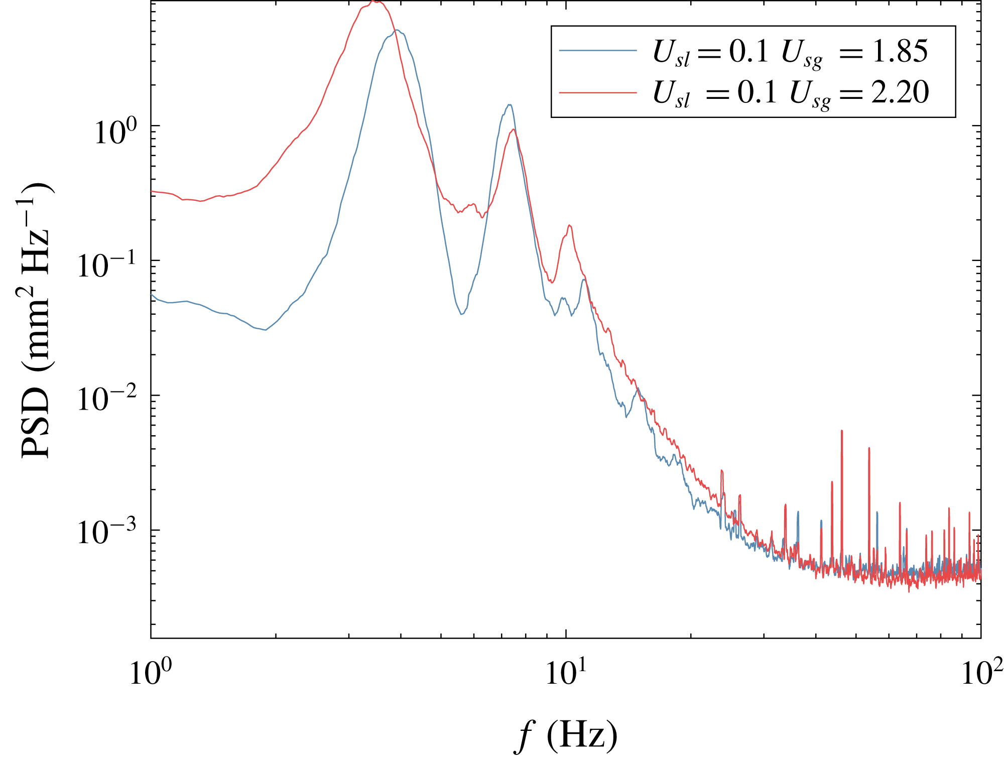
The main characteristics of the two experimental cases are presented in table 1, while the spectra (evaluated by the wave probes) are presented in figure 3;
 $C_{p}$
is the characteristic wave speed evaluated by cross-correlation of the conductance wave probes,
 $\unicode[STIX]{x1D706}_{p}$
is the peak wavelength, evaluated at the peak of the spectrum and
 $\overline{h}$
is the mean water level in the centre of the pipe, evaluated by the wave probes. This is used to evaluate the bulk gas and liquid velocities (
 $U_{bg}/U_{bl}$
). The relationship between the superficial velocity of phase
 $k$
and the bulk velocity is
 $U_{sk}=A_{k}U_{bk}/A$
where
 $A$
and
 $A_{k}$
are the pipe cross-sectional area and the area occupied by phase
 $k$
.
 $\unicode[STIX]{x1D706}_{p}$
and
 $\overline{h}$
implies that
 $k_{p}h\approx 1.3{-}1$
for the two cases considered, and the waves can be classified as waves at intermediate depth. The wave age
 $C_{p}/u_{\ast }$
indicates that the waves are young, wind-driven waves. The interfacial friction velocity
 $u_{\ast }$
was estimated using a force balance over a 12.4 m section of the pipe. Here the average pressure drop in the air phase was measured, and the wall friction was estimated by the Colebrook–White formulation. Subtracting the wall friction forces from the measured pressure drop yields an estimate of the interface friction
 $\unicode[STIX]{x1D70F}_{i}$
, and the friction velocity is then evaluated as
 $u_{\ast }=\sqrt{\unicode[STIX]{x1D70F}_{i}/\unicode[STIX]{x1D70C}}$
. Note that this is a global estimate of the wave age, and as the wave field develops along the pipe, deviations from the values listed in table 1 may occur locally. Further details on the development of the two-phase flow field with varying
 $U_{sg}$
have been discussed by Ayati et al. (Reference Ayati, Kolaas, Jensen and Johnson2015) and Vollestad et al. (Reference Vollestad, Ayati and Jensen2019b
).
Frequency spectra from the wave probes for the two experimental cases.

Overview of experimental cases.
 $N_{PIV}$
is the number of PIV velocity fields analysed for each case.

In the present work, measurements are performed in the pipe centreplane, and flow variations in the lateral direction are not quantified. As discussed by Vollestad et al. (Reference Vollestad, Ayati and Jensen2019b ) the flow rates under investigation are within the ‘2-D wave’ regime defined by Tzotzi & Andritsos (Reference Tzotzi and Andritsos2013). The three-dimensionality of the wavefield (using the same two-phase flow loop) has previously been investigated by Strand (Reference Strand1993) and Smith et al. (Reference Smith, Kolaas, Jensen and Sveen2018). Strand (Reference Strand1993) used conductance wave probes at different cross-wise planes of the pipe and found that for the flow rates under investigation in the present work, the normalized cross-correlation between the centreline and off-axis surface elevation exceeded 0.85 everywhere in the pipe. Smith et al. (Reference Smith, Kolaas, Jensen and Sveen2018) used X-ray tomography and found that the dominant wave components were well-described as two-dimensional for the flow rates of interest. Near the pipe walls the waves were observed to have a crescent shape, and slightly larger wave amplitudes were observed compared with the pipe centreline. This is in line with visual observations of the highest flow rate case in the present work. Example images of breaking and non-breaking waves in the same two-phase pipe flow configuration presented by Vollestad et al. (Reference Vollestad, Ayati and Jensen2019b ) show that the waves retain their 2-D shape also during breaking.
3.2 Regions of interest
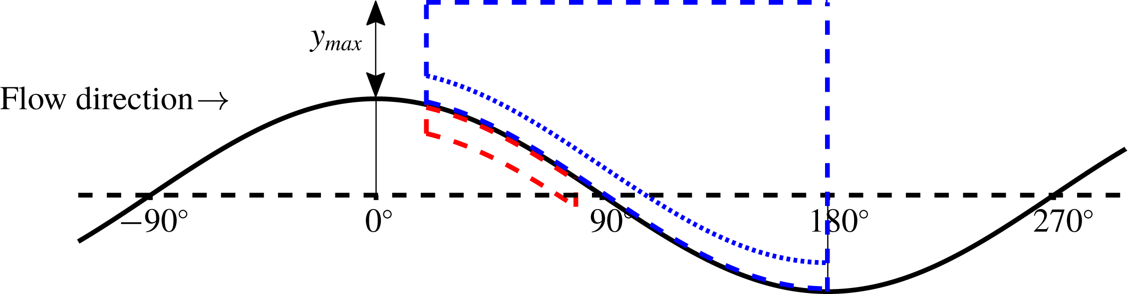
Two ‘regions of interest’ (ROIs) are implemented to monitor the velocity field in the gas and liquid phase, and to identify characteristic features of wave breaking and airflow separation respectively. These are denoted GROI and LROI for the gas and liquid phase ROIs. The ROI location relative to the wave profile is illustrated in figure 4 and described in more detail in the following sections.
The local wave phase
 $\unicode[STIX]{x1D703}$
is used to define the relative location along the wave;
 $\unicode[STIX]{x1D703}$
is determined based on a zero-crossing procedure. The crest/trough were assigned phases of
 $0^{\circ }$
and
 $180^{\circ }$
respectively, while the zero-down/zero-up crossings were assigned phases of
 $90^{\circ }$
and
 $270^{\circ }/-90^{\circ }$
. Phases in between were linearly distributed. This is illustrated in figure 4.
Illustration of the ROIs applied. Red dashed line: liquid-phase ROI to detect wave breaking. Blue dashed line: gas-phase ROI. Blue dotted line: lower boundary of GROI applied when evaluating
 $\unicode[STIX]{x1D714}_{rms,g}$
.

3.2.1 Liquid-phase ROI
The LROI is defined for
 $20^{\circ }<\unicode[STIX]{x1D703}<80^{\circ }$
, from the interface and 3 mm into the liquid phase. The velocity field within the liquid-phase ROI is used to classify waves as either breaking or non-breaking based on the criterion by Vollestad et al. (Reference Vollestad, Ayati and Jensen2019b
). Vollestad et al. (Reference Vollestad, Ayati and Jensen2019b
) monitored the r.m.s. vorticity (denoted
 $\unicode[STIX]{x1D714}_{rms}$
) within the same ROI. Waves with
 $\unicode[STIX]{x1D714}_{rms}<60~\text{s}^{-1}$
were assessed to be non-breaking, while waves with
 $\unicode[STIX]{x1D714}_{rms}>100~\text{s}^{-1}$
were classified as active breaking. As we in the present study apply a spatial resolution closely matching the resolution used in Vollestad et al. (Reference Vollestad, Ayati and Jensen2019b
), and hence resolve a similar fraction of the shear generated by wave breaking, the same criterion is used also here. The r.m.s. vorticity in the LROI is denoted
 $\unicode[STIX]{x1D714}_{rms,l}$
in the remainder of this paper.
Only waves where the full LROI was present in the liquid-phase PIV FOV are analysed further. In table 2 the number of waves where the LROI was present in the liquid PIV FOV (
 $N_{LROI}$
) and the number of breaking and non-breaking waves are presented. Note that waves with
 $60~\text{s}^{-1}<\unicode[STIX]{x1D714}_{rms}<100~\text{s}^{-1}$
are classified as ‘intermediate’, and not counted as either breaking or non-breaking. Further discussions on this methodology for distinguishing actively breaking and non-breaking waves is presented in Vollestad et al. (Reference Vollestad, Ayati and Jensen2019b
).
Number of waves found to be breaking/non-breaking in this study.
 $N_{LROI}$
are number of waves with the full LROI present in the liquid PIV FOV.

3.2.2 Gas-phase ROI
The GROI includes the region from
 $\unicode[STIX]{x1D703}=20^{\circ }$
to
 $180^{\circ }$
. If the full region is not present in the gas-phase FOV, the region from
 $\unicode[STIX]{x1D703}=20^{\circ }$
to the right edge of the FOV is applied as the GROI. The GROI extends to a height
 $y_{max}$
above the crest (
 $y_{max}$
is the crest height relative to the mean water level), i.e.
 $2\ast y_{max}$
above the mean water level.
The purpose of the GROI is to monitor the velocity field for signs of airflow separation. When the shear layer separates from the interface, there is a significant increase in the vorticity away from the interface, and a sheltered region of low air velocity between the interface and the separated shear layer. Two individual measures are included in order to monitor these properties in the GROI:
(i) The characteristic critical height,
$\overline{y_{c}}$
is calculated by the area within the GROI with
$u<C_{p}$
, divided by the horizontal extent of the GROI. Hence,
$\overline{y_{c}}$
represents the mean critical height (height where
$u=C_{p}$
) within the GROI. To remove the effect of wave amplitude we evaluate
$\overline{y_{c}}/y_{max}$
as a normalized measure of the sheltering.(ii) To evaluate the increased vorticity, we extract the r.m.s. vorticity within the GROI, denoted
$\unicode[STIX]{x1D714}_{rms,g}$
. High values of
$\unicode[STIX]{x1D714}_{rms,g}$
are assessed to be related to the detachment of the shear layer and increased turbulence away from the gas–liquid interface.


When evaluating
 $\overline{y_{c}}/y_{max}$
the GROI extends from the interface to its top border (region illustrated by dashed lines in figure 4). When monitoring
 $\unicode[STIX]{x1D714}_{rms,g}$
, we omit the region closest to the interface (from the interface and 3 mm up), as we are interested in detecting signs of the high intensity shear layer separating from the interface, not shear which remains attached to the interface. Hence, the GROI for evaluating
 $\unicode[STIX]{x1D714}_{rms,g}$
is bounded from below by the dotted line in figure 4.
4 Results
4.1 Example instantaneous velocity profiles
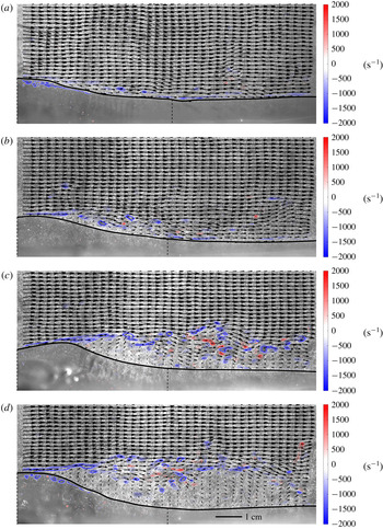
Figure 5 presents instantaneous velocity fields for four waves (referred to as waves A–D). Figure 5(a) shows an example velocity field at
 $U_{sg}=1.85~\text{m}~\text{s}^{-1}$
, while figure 5(b–d) is taken from the
 $U_{sg}$
= 2.20
 $~\text{m}~\text{s}^{-1}$
experimental case. The figures present the velocity vectors in the air phase, along with vorticity contours in both the gas and liquid phase, overlaid the original gas-phase PIV image. Note that the liquid vorticity is multiplied by 10 for visibility.
Example velocity fields. Contours represent vorticity (
 $\text{s}^{-1}$
). NB: liquid vorticity multiplied by 10 for visibility. Showing
 $1/4$
vectors in the gas phase. Dashed vertical lines indicate borders of liquid-phase PIV. Solid black line: interface. Length scale included in (d). (a) Wave A,
 $U_{sg}=1.85~\text{m}~\text{s}^{-1}$
. (b) Wave B,
 $U_{sg}=2.20~\text{m}~\text{s}^{-1}$
. (c) Wave C,
 $U_{sg}=2.20~\text{m}~\text{s}^{-1}$
. (d) Wave D,
 $U_{sg}=2.20~\text{m}~\text{s}^{-1}$
.

For all waves the negative shear layer is seen to remain attached above the wave crest. At the leeward side of the crest the shear layer is seen to separate from the interface, depending on the gas flow rate and wave crest geometry. This effect is most pronounced for the two steepest waves (figure 5 c,d), but also for figure 5(b) a slight detachment of the shear layer, and a sheltered region of low-velocity air is observed on the leeward side of the crest. In figure 5(c,d) regions of negative axial velocity are observed within the sheltered region.
Interface elevation of the four waves displayed in figure 5. Crest positioned at
 $x=0$
.

Overview of parameters describing the wave interface for waves A, B, C and D presented in figure 6.

The vorticity contours from the liquid-phase PIV are also included in figure 5 (superimposed on the gas-phase PIV image). In figure 5(b,c) the vorticity is seen to be low, and evenly distributed along the wave profile, while in figure 5(a,d) there are coherent regions of negative vorticity on the leeward side of the wave and below the crest. This indicates a turbulent spilling region caused by microscale wave breaking, and the waves are assessed to be in a state of active breaking according to the criterion presented in § 3.2. It can be noted that while the wave profile of figure 5(b) is fairly smooth, parasitic capillaries are observed on the leeward side of the wave in figure 5(c). These capillary waves were also observed by Vollestad et al. (Reference Vollestad, Ayati and Jensen2019b ) for steep non-breaking waves in the same experimental conditions. When a wave transitions into an active state of breaking, fluid elements on the leeward side of the crest spill downwards and the capillary waves are displaced downstream of the spilling region (Vollestad et al. Reference Vollestad, Ayati and Jensen2019b ).
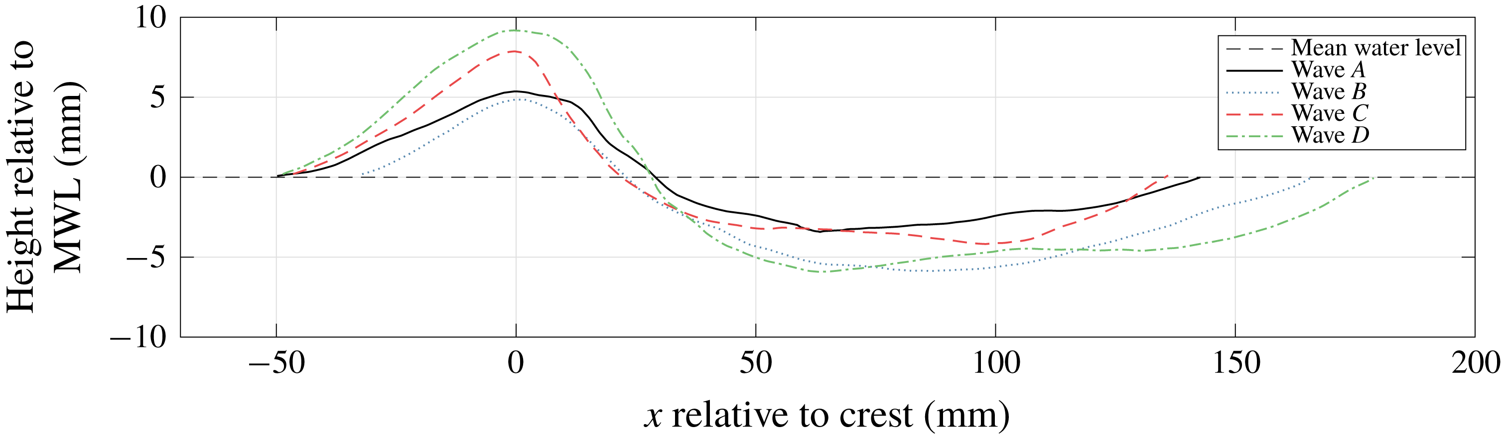
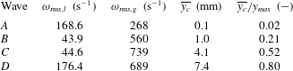
The interfaces of the four waves shown in figure 5 are presented in figure 6. These were obtained from the LFV camera, and hence extend outside of the PIV FOV. Table 3 summarizes key parameters for the waves. Here we use the same notation as Reul et al. (Reference Reul, Branger and Giovanangeli2008):
 $y_{max}$
and
 $y_{min}$
are the maximum and minimum surface elevations, while
 $\unicode[STIX]{x1D706}$
is the wavelength;
 $\unicode[STIX]{x1D716}_{crest}$
is the crest front face (leeward side) steepness (
 $|\unicode[STIX]{x0394}y/\unicode[STIX]{x0394}x|$
from the crest to the zero-down-crossing at
 $\unicode[STIX]{x1D703}=90^{\circ }$
), while
 $\unicode[STIX]{x1D6FF}_{crest}$
is the crest windward side steepness (
 $|\unicode[STIX]{x0394}y/\unicode[STIX]{x0394}x|$
from
 $\unicode[STIX]{x1D703}=-90^{\circ }$
to
 $0^{\circ }$
);
 $\unicode[STIX]{x1D707}$
is the vertical asymmetry factor (
 $\unicode[STIX]{x1D707}=y_{max}/(y_{max}+|y_{min}|)$
), while
 $\unicode[STIX]{x1D706}_{v}$
is the crest horizontal asymmetry factor (
 $\unicode[STIX]{x1D706}_{v}=\unicode[STIX]{x1D716}_{crest}/\unicode[STIX]{x1D6FF}_{crest}$
). The wave steepness
 $ak$
is evaluated as
 $ak=\unicode[STIX]{x03C0}H/\unicode[STIX]{x1D706}$
, where
 $H$
is the wave height (
 $H=y_{max}+|y_{min}|$
).
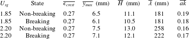
From the data presented in table 3 it can be observed that there is only a moderate difference in the overall wave steepness
 $ak$
comparing the three waves at
 $U_{sg}=2.20~\text{m}~\text{s}^{-1}$
. The front face steepness
 $\unicode[STIX]{x1D716}_{crest}$
is however significantly higher for waves C and D.
Table 4 presents the results for the parameters discussed in § 3.2. It can be seen that
 $\unicode[STIX]{x1D714}_{rms,l}$
varies by a factor four from the non-breaking to breaking cases, and that following the criterion presented in § 3.2, waves A and D are in a state of active breaking, while B and C are non-breaking.
The normalized critical height is seen to increase through waves A–D, from close to 0 for wave A to 0.8 for wave D. This is in accordance with the visual impression obtained from figure 5, as the sheltered region below the separated shear layer is seen to increase from waves A to D. We observe that
 $\unicode[STIX]{x1D714}_{rms,g}$
for wave A is significantly lower than the three other waves. This is to be expected, as wave A is from the
 $U_{sg}=1.85~\text{m}~\text{s}^{-1}$
case, where the shear on the gas–liquid interface is lower, and as the shear layer is seen to remain attached along the wave profile. While
 $\overline{y_{c}}/y_{max}$
is maximum for wave D,
 $\unicode[STIX]{x1D714}_{rms,g}$
is higher for wave C. Comparing figure 5(c,d) the region of high intensity shear is seen to be somewhat thicker above wave C, indicating a higher degree of turbulent mixing.
Overview of results from the ROI analysis for the four waves.

The results in this section provide some indications of the importance of the crest geometry to the structure of the airflow. However, analysing the effect of individual wave profile parameters and the effect of breaking requires a statistical approach.
4.2 Airflow statistics over breaking and non-breaking waves
In this section, statistics of
 $\overline{y_{c}}/y_{max}$
and
 $\unicode[STIX]{x1D714}_{rms,g}$
above breaking and non-breaking waves are presented. To isolate the effect of active wave breaking from the geometrical properties of the waves, it is necessary to keep at least one of the geometrical properties of the waves constant, as the wave geometry obviously has a significant impact on the airflow.
Reul et al. (Reference Reul, Branger and Giovanangeli2008) characterized the extent of the separated region by the air velocity, crest height and
 $\unicode[STIX]{x1D716}_{crest}$
. Here, we isolate the air velocity by comparing each of the experimental cases individually. As the vertical extent of the GROI used to evaluate
 $\unicode[STIX]{x1D714}_{rms,g}$
, and
 $\overline{y_{c}}/y_{max}$
is scaled by the local crest height,
 $\unicode[STIX]{x1D716}_{crest}$
is chosen as the geometrical property of the wave to keep constant. Note that the average wave profile of breaking and non-breaking waves with the same
 $\unicode[STIX]{x1D716}_{crest}$
will vary, as wave breaking modifies the geometrical properties of the waves. Hence, completely isolating the effect of active wave breaking from the geometrical properties of individual waves is not possible. The variations on the overall wave form for breaking and non-breaking waves at constant
 $\unicode[STIX]{x1D716}_{crest}$
and their effect on the results are discussed in § 5.
Breaking and non-breaking waves were evaluated individually, and binned in
 $\unicode[STIX]{x1D716}_{crest}$
intervals of 0.05. For each
 $\unicode[STIX]{x1D716}_{crest}$
-interval with more than five observations the mean value, standard deviation and 95 % confidence interval of the mean value (evaluated by the
 $t$
distribution) of
 $\overline{y_{c}}/y_{max}$
and
 $\unicode[STIX]{x1D714}_{rms,g}$
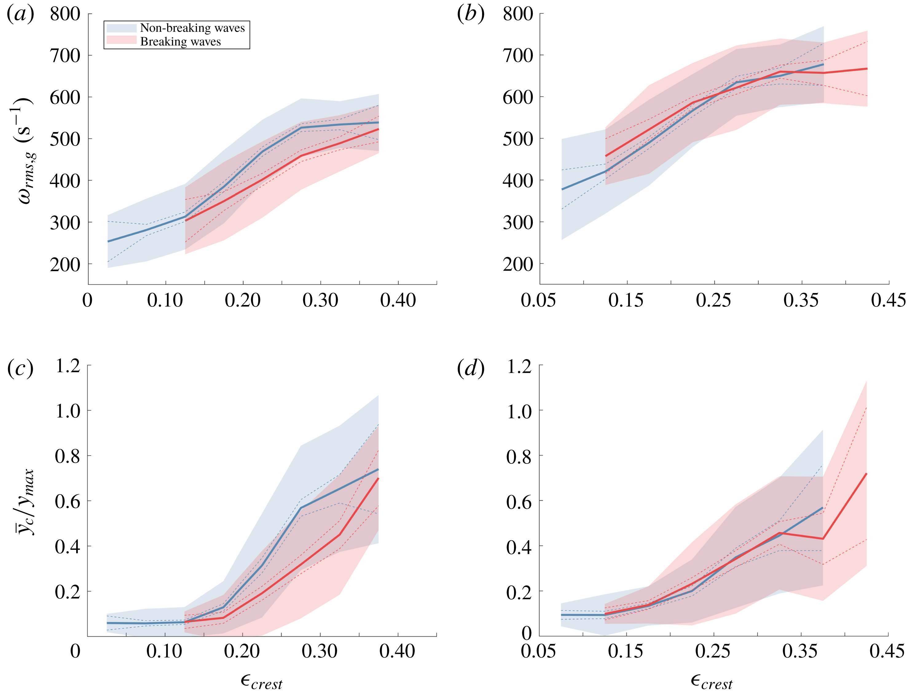
are evaluated. Results are presented in figure 7.
Statistics of
 $\unicode[STIX]{x1D714}_{rms,g}$
(a,b) and
 $\overline{y_{c}}/y_{max}$
(c,d) as a function of
 $\unicode[STIX]{x1D716}_{crest}$
. Thick full line: mean value, dashed line: 95 % confidence interval of mean value, shaded colour: mean value
 $\pm$
standard deviation.
 $U_{sg}=1.85~\text{m}~\text{s}^{-1}$
(a,c), and
 $U_{sg}=2.20~\text{m}~\text{s}^{-1}$
(b,d).

The results in figure 7 show that both
 $\unicode[STIX]{x1D714}_{rms,g}$
and
 $\overline{y_{c}}/y_{max}$
are strongly correlated with
 $\unicode[STIX]{x1D716}_{crest}$
. As expected, increased
 $\unicode[STIX]{x1D716}_{crest}$
is seen to result in increased turbulence and larger areas of sheltered airflow on the leeward side of the crest. It can be noted that all waves with
 $\unicode[STIX]{x1D716}_{crest}<0.1$
are found to be non-breaking, while the steepest waves at
 $U_{sg}=2.20~\text{m}~\text{s}^{-1}$
are found to be breaking. The shaded area represents the standard deviation around the mean value, and significant deviations around the mean value are observed both for breaking and non-breaking waves.
Results for the
 $U_{sg}=2.20~\text{m}~\text{s}^{-1}$
case show that the breaking and non-breaking cases are more or less overlapping. The 95 % confidence intervals are everywhere overlapping, indicating that while there are some indications that
 $\unicode[STIX]{x1D714}_{rms,g}$
is higher for breaking waves within the steepness interval of
 $0.1<\unicode[STIX]{x1D716}_{crest}<0.25$
, these results are not considered statistically significant.
At
 $U_{sg}=1.85~\text{m}~\text{s}^{-1}$
there is a significant difference in the statistics above breaking and non-breaking waves. In the interval
 $0.2<\unicode[STIX]{x1D716}_{crest}<0.35$
, the non-breaking waves are observed to result in significantly higher
 $\unicode[STIX]{x1D714}_{rms,g}$
and
 $\overline{y_{c}}/y_{max}$
. This indicates that within this steepness interval, active wave breaking reduces the intensity of shear layer separation, as both the sheltered region and the turbulence generated by the separated shear layer are reduced. This is a somewhat surprising result as wave breaking is typically assessed to enhance the airflow separation above waves.
While the results presented in this section are indicative of the effect of active wave breaking for the cases considered, further analysis of the experimental data is needed to understand how the variations in
 $\unicode[STIX]{x1D714}_{rms,g}$
and
 $\overline{y_{c}}/y_{max}$
observed for the
 $U_{sg}=1.85~\text{m}~\text{s}^{-1}$
case manifest in the average flow field above breaking and non-breaking waves.
4.3 Analysis of effect of breaking for
$0.225<\unicode[STIX]{x1D716}_{crest}<0.325$

In this section we perform an analysis of the velocity fields above breaking and non-breaking waves within the steepness interval
 $0.225<\unicode[STIX]{x1D716}_{crest}<0.325$
, i.e. within the interval where we, in § 4.2, observed a reduced sheltering due to active wave breaking in the
 $U_{sg}=1.85~\text{m}~\text{s}^{-1}$
case. The analysis is performed both for the
 $U_{sg}=1.85$
and
 $2.20~\text{m}~\text{s}^{-1}$
cases, to further describe the effect of active wave breaking observed in § 4.2. In § 4.3.1 a conditional phase averaging of the velocity fields is performed, while in § 4.3.2 the spectra above breaking and non-breaking waves are analysed.
While
 $\unicode[STIX]{x1D716}_{crest}$
is kept constant, other properties of the waves will vary slightly comparing breaking and non-breaking waves. The mean properties of the waves under investigation are presented in table 5. It is observed that while the average front face steepness
 $\unicode[STIX]{x1D716}_{crest}$
is equal, the average crest height
 $y_{max}$
and wave height
 $H$
for non-breaking waves are somewhat higher than for the breaking waves. These variations will be discussed in § 5.
Mean properties of the four averaging cases under investigation.

4.3.1 Phase-averaged results
A conditional phase averaging of the gas and liquid phases is performed. The wave-following coordinate system is described in the Appendix. The coordinate system in the liquid phase is the same as the coordinate system employed by Vollestad et al. (Reference Vollestad, Ayati and Jensen2019b ) to evaluate phase-averaged statistics of the liquid phase of microscale breaking waves, while the wave-following coordinate system in the gas phase is similar to the coordinate system used by Vollestad et al. (Reference Vollestad, Ayati, Angheluta, LaCasce and Jensen2019a ), analysing airflow over waves.
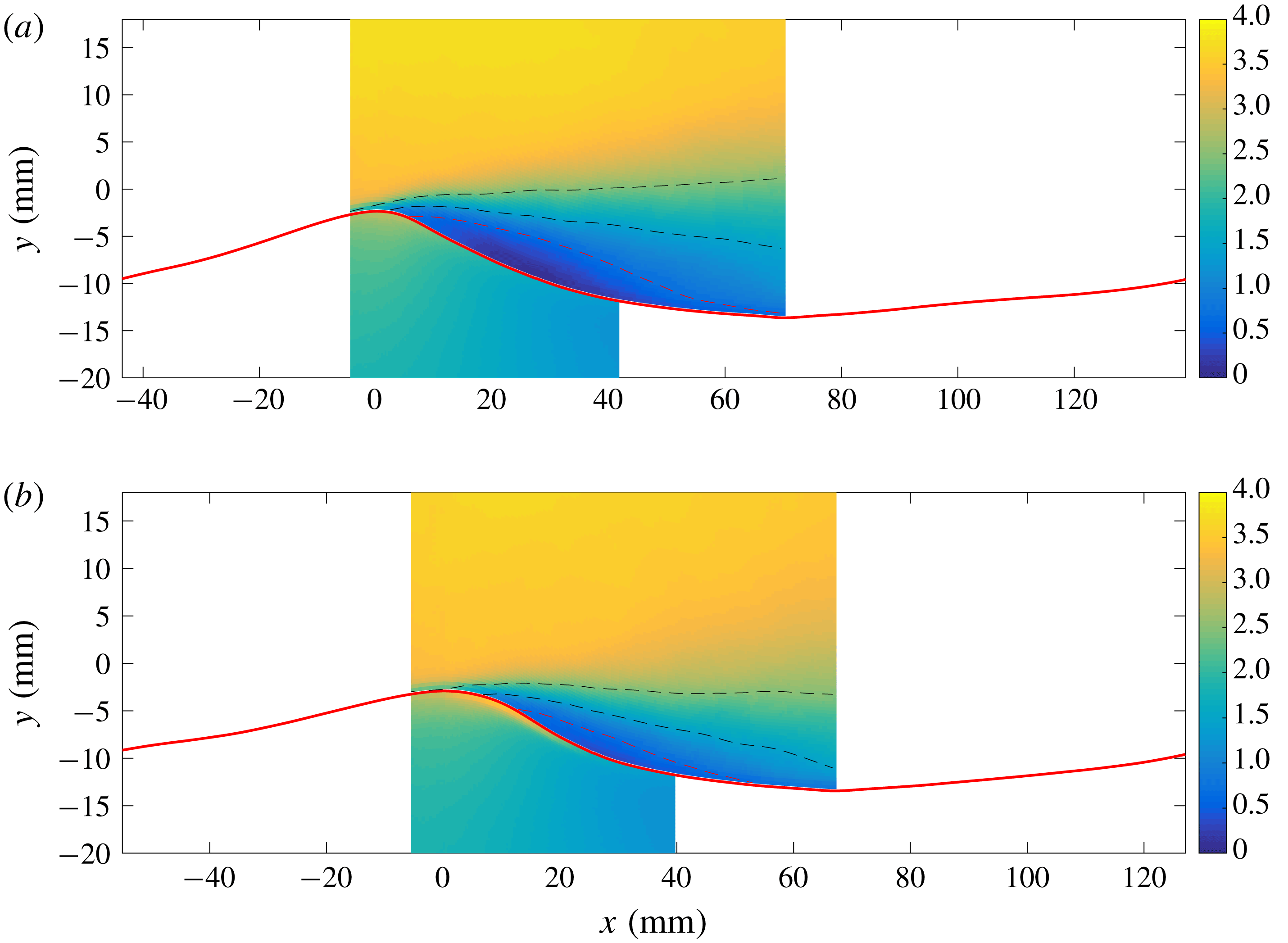
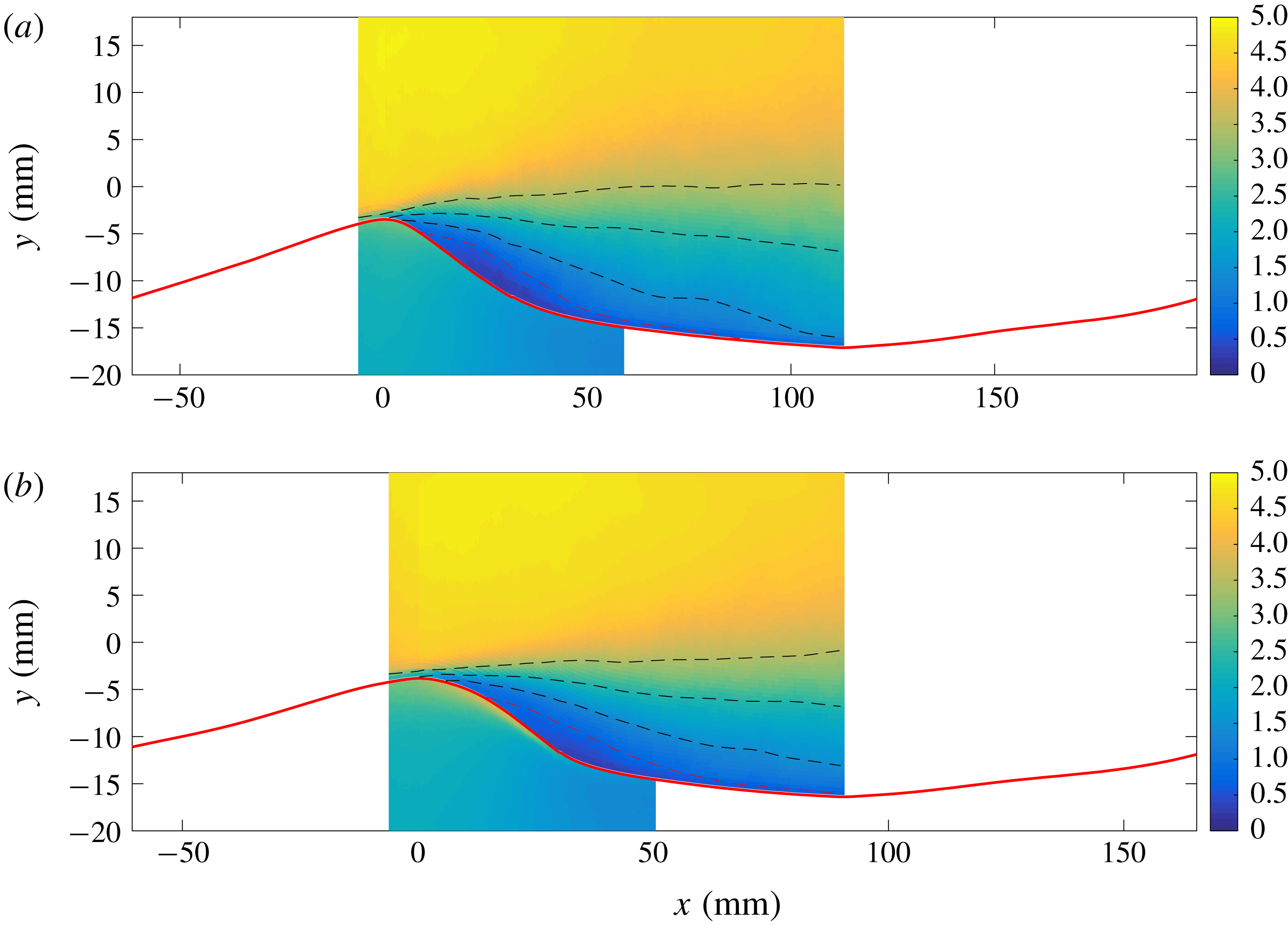
Figures 8 and 9 present the phase-averaged horizontal velocity (
 $\langle u\rangle$
) for the
 $U_{sg}=1.85$
and
 $2.20~\text{m}~\text{s}^{-1}$
cases respectively. Breaking and non-breaking waves are averaged individually. Due to the limited FOV of the PIV cameras and the triggering applied (cf. § 2), the region where we can obtain reliable phase-averaged velocity profiles is limited to approximately
 $-10^{\circ }<\unicode[STIX]{x1D703}<180^{\circ }$
for the gas phase and
 $-10^{\circ }<\unicode[STIX]{x1D703}<120^{\circ }$
for the liquid phase. Here more than 100 data points are used in the evaluation of each phase-averaged quantity. In the range
 $20^{\circ }<\unicode[STIX]{x1D703}<80^{\circ }$
(LROI), more than 200 data points are obtained (number decreasing with distance from LROI). While the phase-averaged velocity profiles are not fully converged, the main flow features, such as the extent of the sheltered region, are assessed to be qualitatively converged, as performing the averaging with half of the available data resulted in only minor deviations from the results presented in figures 8 and 9, and no qualitative change in the results or conclusions related to the phase-averaged flow fields.
The results are overlaid on the average interface (evaluated individually for breaking and non-breaking waves) detected by the LFV camera. Isocurves of constant velocity are included in the gas-phase velocity field. The critical height (where
 $\langle u\rangle =C_{p}$
) is illustrated by a red dashed line.
Phase-averaged results for the horizontal velocity
 $\langle u\rangle$
, converted to (
 $x,y$
)-coordinates by applying the mean interface elevation for each case. Gas-phase results plotted for
 $-10^{\circ }<\unicode[STIX]{x1D703}<180^{\circ }$
. Liquid-phase horizontal velocity multiplied by 5 for visibility. Colour bar in
 $\text{m}~\text{s}^{-1}$
. Full red line indicates mean interface elevation. Red dashed line represents the critical height, where
 $\langle u\rangle =C_{p}$
. Black dashed lines represent isocurves at 1.5 and
 $2.5~\text{m}~\text{s}^{-1}$
. (a)
 $U_{sg}=1.85~\text{m}~\text{s}^{-1}$
, non-breaking, (b)
 $U_{sg}=1.85~\text{m}~\text{s}^{-1}$
, breaking.

Phase-averaged results for the horizontal velocity
 $\langle u\rangle$
, converted to (
 $x,y$
)-coordinates by applying the mean interface elevation for each case. Gas-phase results plotted for
 $-10^{\circ }<\unicode[STIX]{x1D703}<180^{\circ }$
. Liquid-phase horizontal velocity multiplied by 5 for visibility. Colour bar in
 $\text{m}~\text{s}^{-1}$
. Full red line indicates mean interface elevation. Red dashed line represents the critical height, where
 $\langle u\rangle =C_{p}$
. Black dashed lines represent isocurves at 1.5, 2.5 and
 $3.5~\text{m}~\text{s}^{-1}$
. (a)
 $U_{sg}=2.20~\text{m}~\text{s}^{-1}$
, non-breaking. (b)
 $U_{sg}=2.20~\text{m}~\text{s}^{-1}$
, breaking.

The results in figure 8 show that the airflow is more sheltered in the lee of the non-breaking waves compared with the breaking waves. While the critical height is seen to detach from the interface close to the crest for the non-breaking case, the detachment occurs later over breaking waves, and the area where
 $\langle u\rangle <C_{p}$
is significantly reduced. It can be noted that while the peak horizontal velocity in the liquid phase of the non-breaking wave is centred below the crest, the peak is shifted towards the leeward side of the breaking waves. This is a clear indication of the spilling region observed below breaking waves. One interpretation of the results is that the spilling motion of the liquid on the leeward side of the wave reduces the shear on the gas flow, or even helps accelerate the gas close to the surface as the spilling is initiated, thus reducing the sheltered region on the leeward side of the wave.
The results presented in figure 9 show that the effect of breaking is less pronounced for the
 $U_{sg}=2.20~\text{m}~\text{s}^{-1}$
case compared with the lower gas flow rate case. Again the critical height is seen to detach from the interface somewhat further downwind on the wave profile for the breaking case, but the sheltered area (here evaluated as the area limited by
 $\langle u\rangle <C_{p}$
) is very similar, comparing the breaking and non-breaking cases.
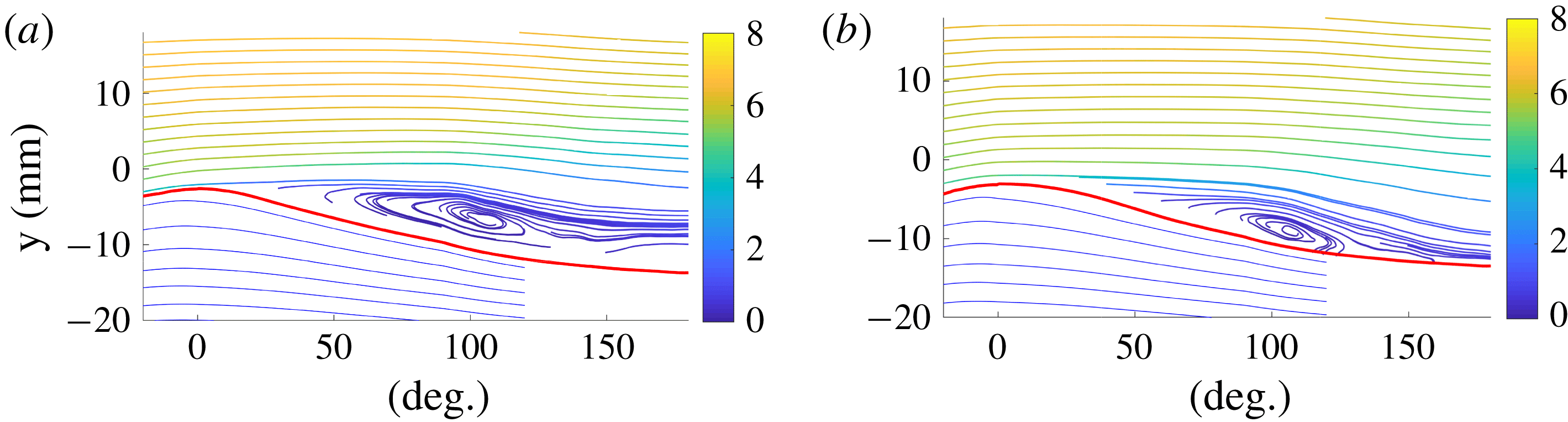
In figure 10, streamlines of the phase-averaged velocity fields, observed in a frame of reference moving with the characteristic wave speed
 $C_{p}$
, are presented for the
 $U_{sg}=1.85~\text{m}~\text{s}^{-1}$
case. For both the breaking and non-breaking wave cases a clear ‘cat’s eye’ structure is observed on the leeward side of the crest. This illustrates that as the waves propagate in the streamwise direction, they experience a co-moving pocket of air in its front, displacing the streamlines in the outer flow relative to the wave profile. In table 6 the location of the cat’s eye centre (
 $\unicode[STIX]{x1D703}_{c}$
,
 $\unicode[STIX]{x1D709}_{c}$
, where
 $\unicode[STIX]{x1D709}_{c}$
is the height above the interface) and the area under the critical height
 $y_{c}$
are summarized for all four averaging cases. The results show that while the sheltered area below non-breaking waves is slightly larger compared with the breaking waves at
 $U_{sg}=2.20~\text{m}~\text{s}^{-1}$
, the effect is much more pronounced for the lower gas flow rate, and the area below the critical height is observed to be three times larger for the non-breaking waves at
 $U_{sg}=1.85$
compared with breaking waves of similar
 $\unicode[STIX]{x1D716}_{crest}$
. These results are consistent with the results obtained in § 4.2, where it was found that
 $\overline{y_{c}}/y_{max}$
was significantly reduced as a result of breaking for the
 $U_{sg}=1.85~\text{m}~\text{s}^{-1}$
case.
Gent & Taylor (Reference Gent and Taylor1977) included an increased surface drift velocity to numerically analyse the effect of wave breaking on the extent of the cat’s eye centre. Analysing a strongly forced wave (
 $c/u_{\ast }\approx 1.5$
) they found that the effect of the increased surface drift was to reduce the elevation of the cat’s eye centre by approximately 30 %. While this is qualitatively in agreement with the results observed for the
 $U_{sg}=1.85~\text{m}~\text{s}^{-1}$
case, the waves considered by Gent & Taylor (Reference Gent and Taylor1977) had an even lower wave age than the cases considered in this work, hence the
 $U_{sg}=2.20~\text{m}~\text{s}^{-1}$
case should be the more comparable. However, here we do not observe any significant change in the elevation of the cat’s eye centre.
Streamlines of phase-averaged velocity fields seen in a frame of reference moving with the characteristic wave speed
 $C_{p}$
(
 $\langle \boldsymbol{u}\rangle -C_{p}$
) for the
 $U_{sg}=1.85~\text{m}~\text{s}^{-1}$
case. Gas-phase streamlines coloured by
 $0.5(\langle u\rangle ^{2}+\langle v\rangle ^{2})$
(
 $\text{m}^{2}~\text{s}^{-2}$
). (a) Non-breaking. (b) Breaking.

Phase-averaged results.
 $\unicode[STIX]{x1D703}_{c}$
and
 $\unicode[STIX]{x1D709}_{c}$
are the wave phase and height above the interface of the cat’s eye centre.

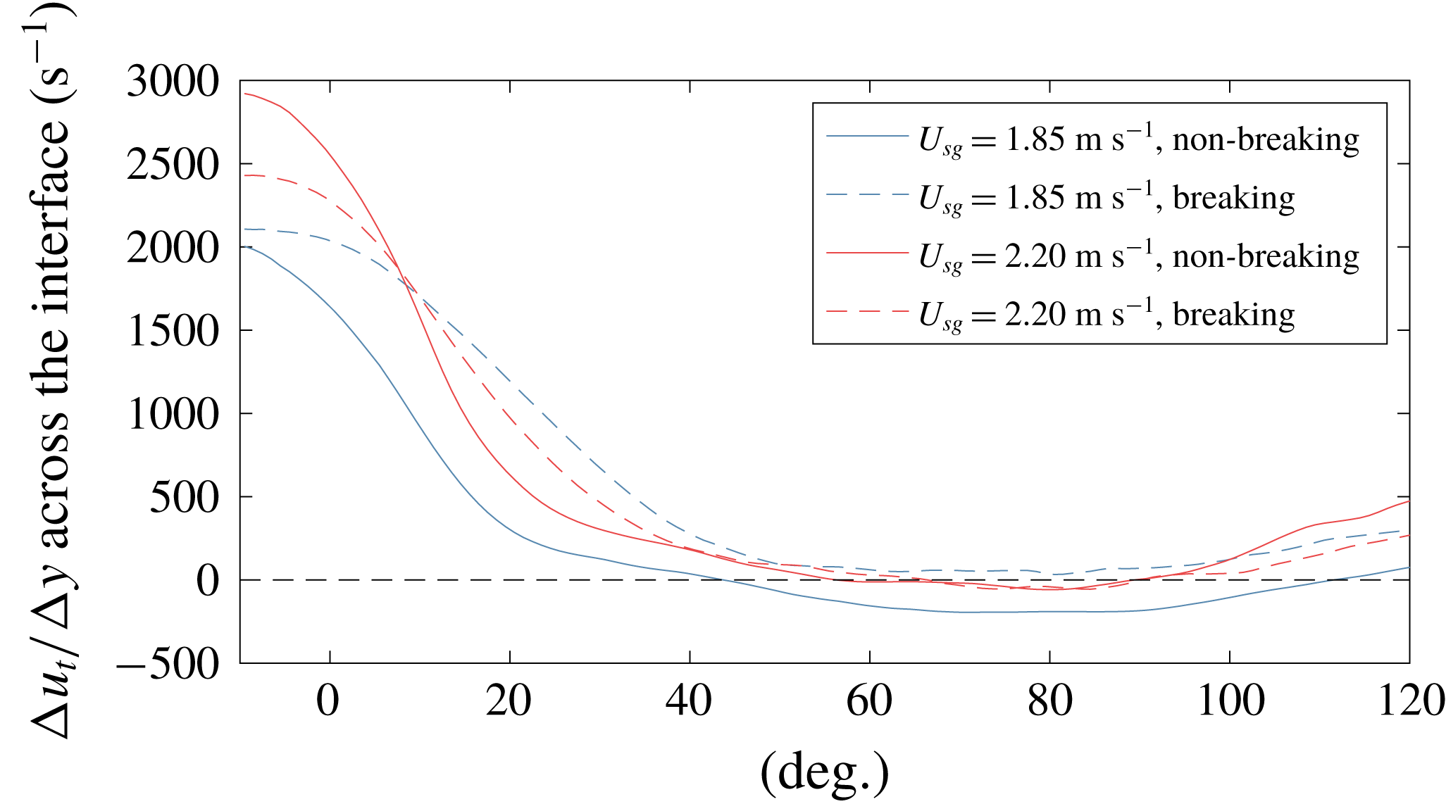
The tangential velocity
 $u_{t}$
along the interface was evaluated for each PIV velocity field, and phase-averaged similarly to the horizontal and vertical velocity components. Due to limitations in the spatial resolution and the accuracy of the interface detection, we are not able to evaluate the tangential shear in the viscous sublayer. Instead, we evaluate the average tangential velocity over the two velocity vectors closest to the interface, in both the gas and liquid phases, and compute
 $\unicode[STIX]{x0394}u_{t}/\unicode[STIX]{x0394}y$
across the interface. While this does not provide the shear stresses directly, the results are indicative of the development of the shear stress along the wave profiles. Results are presented in figure 11. Note that the results are plotted for
 $-10^{\circ }<\unicode[STIX]{x1D703}<120^{\circ }$
, as reliable phase-averaged velocities in both the gas and liquid phases are required.
The results presented in figure 11 indicate that the shear stress at the interface varies considerably between the four averaging cases. The value of
 $\unicode[STIX]{x0394}u_{t}/\unicode[STIX]{x0394}y$
drops off faster for the non-breaking compared to the breaking waves, and for the non-breaking waves at
 $U_{sg}=1.85~\text{m}~\text{s}^{-1}$
the results shows that there is a significant region of the wave profile (
 $50^{\circ }<\unicode[STIX]{x1D703}<110^{\circ }$
) where the liquid on average travels faster than the overlying air, and will exert a force on the gas phase in the streamwise direction.
Value of
 $\unicode[STIX]{x0394}u_{t}/\unicode[STIX]{x0394}y$
over the interface, plotted in the interval
 $-10^{\circ }<\unicode[STIX]{x1D703}<120^{\circ }$
.

From figure 11 we also can observe that the velocity gradient across the interface at the crest is higher for non-breaking than breaking waves at
 $U_{sg}=2.20~\text{m}~\text{s}^{-1}$
. Analysing the phase-averaged velocity fields, it was found that the main reason for this discrepancy was a higher gas velocity close to the interface for the non-breaking waves, not an increased liquid velocity caused by wave breaking. The reason for this behaviour is not completely understood, but it might be related to the somewhat higher crest height of the non-breaking waves compared with the breaking waves under investigation (cf. table 5), as the lower amplitude breaking waves may to a larger degree be sheltered by upwind waves. It is also possible that local interface variations on the windward side of the waves are the reason for these deviations, as the phase-averaged interface profiles indicate that the non-breaking waves are locally steeper close to the wave crest of the windward side compared with the breaking waves. This may result in a higher acceleration of the flow near the crest for non-breaking compared with breaking waves at
 $U_{sg}=2.20~\text{m}~\text{s}^{-1}$
.
The momentum flux at the interface is governed both by shear stresses and form drag. As the experimental set-up does not facilitate measurements of the pressure along the interface, we are not able to infer the overall change in the momentum flux as a result of active breaking. As we consider young waves the critical height is located within the inner region, where the turbulent eddies are in local equilibrium (Belcher & Hunt Reference Belcher and Hunt1993, Reference Belcher and Hunt1998). In this region the turbulent shear stresses displace the streamlines asymmetrically, and the phase shift of the pressure field cannot be inferred directly from the location of the cat’s eye (Kihara et al. Reference Kihara, Hanazaki, Mizuya and Ueda2007).
From the air–sea literature it is well established that form drag contributes to the majority of the wind stress at the wave ages considered in this work (Banner & Peirson Reference Banner and Peirson1998; Sullivan et al.
Reference Sullivan, Banner, Morison and Peirson2018a
,Reference Sullivan, Banner, Morison and Peirson
b
). While the pipe walls will influence the pressure distribution relative to the pressure field above waves in an open system, it is considered likely that this will also be the case for the current experimental investigation. Hence, the total momentum flux may well be higher for non-breaking compared with breaking waves at
 $U_{sl}=1.85~\text{m}~\text{s}^{-1}$
, despite the reduced shear stress.
4.3.2 Spectra above breaking and non-breaking waves
The results in § 4.2 showed that
 $\unicode[STIX]{x1D714}_{rms,g}$
was higher over non-breaking than breaking waves at
 $U_{sg}=1.85~\text{m}~\text{s}^{-1}$
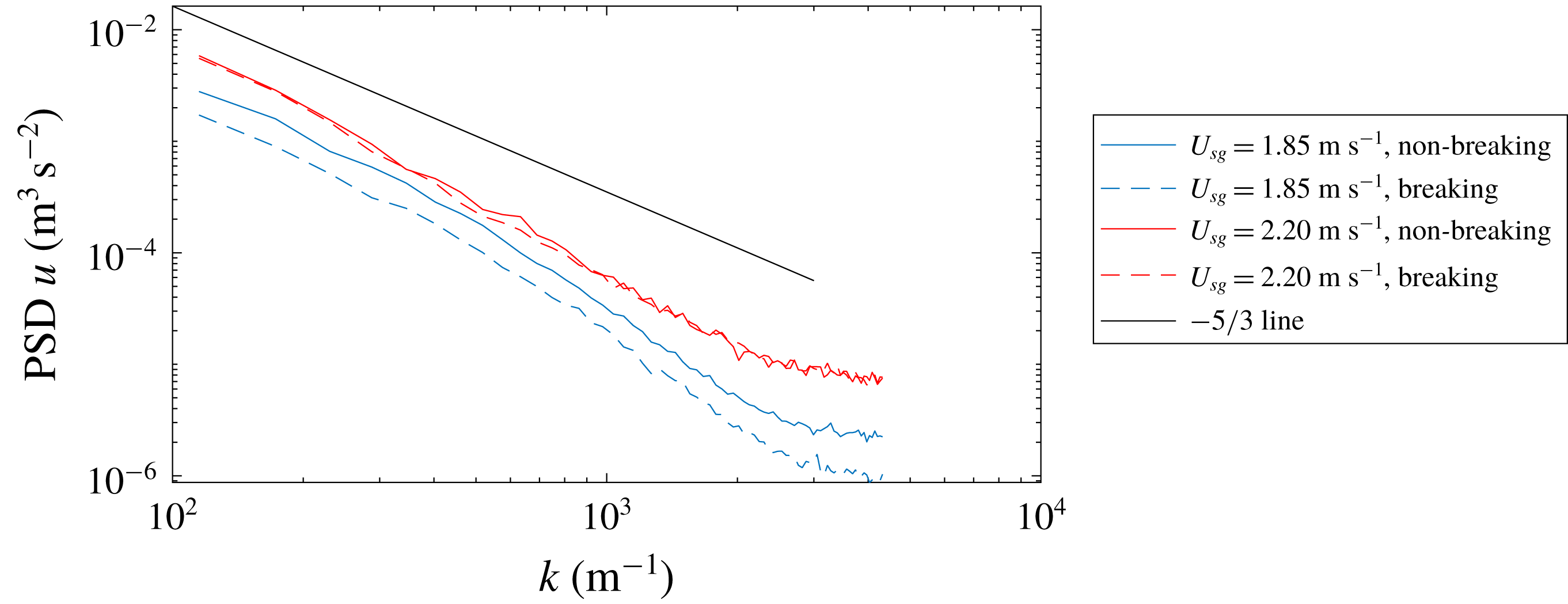
. This is assessed to be related to increased turbulence intensity on the leeward side of the wave. To further investigate the turbulence above breaking and non-breaking waves, the wavenumber spectra of the horizontal velocity fluctuations are evaluated above breaking and non-breaking waves individually. Again we limit the cases under investigation to a steepness interval of
 $0.225<\unicode[STIX]{x1D716}_{crest}<0.325$
. The horizontal velocity 1 mm above the wave crest is extracted for each wave. The periodogram is evaluated for each velocity profile and the mean of the periodogram is used to estimate the horizontal velocity spectra. Results are presented in figure 12.
Power spectral density of the horizontal velocity component (PSD
 $u$
), evaluated 1 mm above the crest of each wave observed with
 $0.225<\unicode[STIX]{x1D716}_{crest}<0.325$
.

From the spectra it can be observed that at
 $U_{sg}=1.85~\text{m}~\text{s}^{-1}$
, the airflow is more fluctuating over non-breaking than breaking waves. At
 $U_{sg}=2.10~\text{m}~\text{s}^{-1}$
the spectra over breaking and non-breaking waves are seen to be more or less equal. This was also observed when the spectra were evaluated at a fixed height (
 $y=5$
mm).
These results are consistent with the results obtained in § 4.2, and indicate that active wave breaking has the effect of reducing the turbulence levels above the wave trough for moderate wind speeds. We relate this to a reduction in the frequency and/or extent of airflow separation on the leeward side of the crest, which could be a result of a change in the wave geometry as the waves transition from non-breaking to breaking, and/or of the spilling motion induced by wave breaking (this will be discussed in § 5). At the higher airflow rate considered (
 $U_{sg}=2.20~\text{m}~\text{s}^{-1}$
), the effect is not observed, and again we conclude that active wave breaking does not significantly influence the airflow above waves at
 $U_{sg}=2.20~\text{m}~\text{s}^{-1}$
.
5 Discussion
In this study efforts have been made to isolate the effect of wave breaking, by comparing breaking and non-breaking waves with similar geometrical properties (with focus on
 $\unicode[STIX]{x1D716}_{crest}$
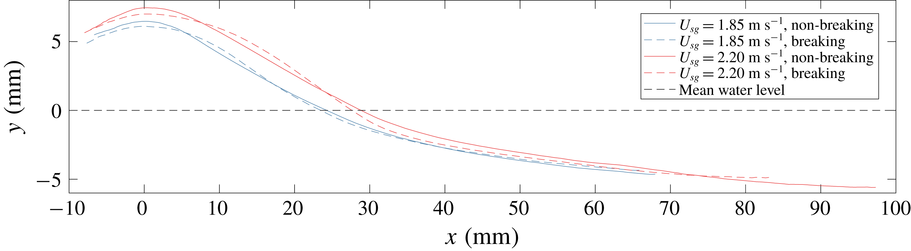
). However, completely isolating the effect of the turbulent spilling region of the liquid is not possible, as wave breaking modifies the interface of the waves. In figure 13 the phase-averaged interface for the four averaging cases analysed in § 4.3 is presented. Results are presented for
 $\unicode[STIX]{x1D703}$
in the range of
 $-20^{\circ }$
to
 $180^{\circ }$
.
Figure 13 shows that, while the waves are evaluated within a narrow
 $\unicode[STIX]{x1D716}_{crest}$
-band, there is a distinct difference in the average interface shape of breaking and non-breaking waves. The non-breaking waves are observed to be somewhat taller, with a higher local steepness close to the wave crest compared with the breaking waves at similar
 $\unicode[STIX]{x1D716}_{crest}$
. The more rounded profile of the breaking waves may help explain why we observe a reduced sheltered region on the leeward side of the breaking waves at
 $U_{sg}=1.85~\text{m}~\text{s}^{-1}$
, as the more gentle slope of the interface may facilitate flow expansion without separation close to the crest. A more direct explanation for the observations made is that the spilling motion of the liquid (observed in the phase-averaged velocity profiles presented in figures 8 and 9) reduces the interfacial shear on the leeward side of the wave, preventing flow separation. Isolating these effects (the spilling motion induced by breaking and the change in wave shape also due to breaking) is not possible when considering naturally occurring wind-generated waves. Numerical analyses or controlled experiments with artificially generated waves are necessary to evaluate which of these effects is dominant in reducing the sheltered region behind breaking waves at the lower gas flow rate.
Mean interface of averaging cases, interval from
 $\unicode[STIX]{x1D703}=-20^{\circ }$
to
 $180^{\circ }$
converted to world coordinates.

It is important to note that all the results in the present work are obtained from, and only valid for, the centreplane of a two-phase pipe flow configuration. The closed pipe geometry induces lateral velocity variations which are not found in open wind–wave tanks, and the wave-coherent pressure variations at the upper pipe wall will be reflected down, modifying the wave-coherent pressure field relative to airflow over waves in an open channel. However, in the trough-to-crest region of the pipe centreline (where we focus our attention) the airflow is primarily influenced by the gas–liquid interface (as the distance to the pipe walls is much larger than the distance to the interface), and the lateral variations are much smaller than in the cross-sections near the pipe walls. As the relationship between active wave breaking and airflow separation has not previously been investigated in a pipe flow configuration, and as the wave breaking process and airflow above waves in pipes have previously been found to have many features similar to air–sea interactions (Vollestad et al. Reference Vollestad, Ayati, Angheluta, LaCasce and Jensen2019a ,Reference Vollestad, Ayati and Jensen b ), it is considered expedient to compare (in a qualitative manner) the results obtained in this work with studies conducted in an open channel.
Numerical results by Sullivan et al. (Reference Sullivan, Banner, Morison and Peirson2018b
), simulating wind over waves representing incipient and active breaking, indicate that the overall wave steepness, not the increased drift velocity or the local steepness variations between incipient and actively breaking waves, is the main parameter controlling the form drag. The simulations by Sullivan et al. (Reference Sullivan, Banner, Morison and Peirson2018b
) are for a wave age which is even lower than the
 $U_{sg}=2.20~\text{m}~\text{s}^{-1}$
case, hence the effect of active wave breaking observed for the
 $U_{sg}=1.85~\text{m}~\text{s}^{-1}$
case is not necessarily in contradiction with the numerical results by Sullivan et al. (Reference Sullivan, Banner, Morison and Peirson2018b
). The results in this work indicate that the effect of wave breaking is relatively more important to the overlying airflow at lower gas flow rates.
Reul et al. (Reference Reul, Branger and Giovanangeli2008) attributed the change in the separated flow region to the front face steepness (
 $\unicode[STIX]{x1D716}_{crest}$
). It is interesting to note their figure 10, depicting two waves at
 $c/u_{\ast }\approx 2.6$
(closely matching the
 $U_{sg}~1.85~\text{m}~\text{s}^{-1}$
case). While the airflow clearly separates over one wave at incipient breaking (
 $\unicode[STIX]{x1D716}_{crest}=0.52$
), it remains attached over the other wave profile (
 $\unicode[STIX]{x1D716}_{crest}=0.28$
), which appears to be in a state of active wave breaking. While Reul et al. (Reference Reul, Branger and Giovanangeli2008) observe a clear correlation between both the horizontal and vertical extents of the separation bubble with
 $\unicode[STIX]{x1D716}_{crest}$
(which one can expect also from the results presented in § 4.2 in the present work), there is considerable scatter in the results, and the results for the
 $U_{sg}=1.85~\text{m}~\text{s}^{-1}$
case in the present work could indicate that the state of breaking, as well as the crest front face steepness, influences the extent of the separated zone. This was however not investigated by Reul et al. (Reference Reul, Branger and Giovanangeli2008).
Investigating the effect of wave breaking on even lower gas flow rates would be of interest. However, as the first signs of microscale wave breaking are observed at
 $U_{sg}=1.80~\text{m}~\text{s}^{-1}$
(Vollestad et al.
Reference Vollestad, Ayati and Jensen2019b
), this would require a different experimental set-up.
6 Concluding remarks
In this work we have performed simultaneous two-phase PIV with the aim of detecting the influence of microbreaking on the airflow above waves in stratified gas–liquid pipe flow. Using the criterion for separating actively breaking and non-breaking waves by Vollestad et al. (Reference Vollestad, Ayati and Jensen2019b ), we analyse the effect of active wave breaking from microscale breaking waves on the airflow structure.
Results show that at the lowest gas flow rate considered (
 $U_{sg}=1.85~\text{m}~\text{s}^{-1}$
), wave breaking has a stabilizing effect on the airflow above the waves, reducing the extent of the separated flow region and the turbulence above the waves. Hence, the effect of airflow separation is reduced over actively breaking waves at this moderate flow rate. At
 $U_{sg}=2.20~\text{m}~\text{s}^{-1}$
the effect of wave breaking is observed to be more moderate. The results indicate that the region in the flow map where active wave breaking significantly influences the air flow field in two-phase pipe flow is relatively small.
While a direct application of the results is restricted to a two-phase pipe flow configuration, the results can also be related to phenomena occurring in the ocean. The impact of wave breaking on the airflow is still a topic under investigation, and the present work adds new insight into the coupling between small scale wave breaking events and airflow separation at high wind forcing.
Acknowledgement
The authors wish to acknowledge the strategic research initiative EarthFlows at the Faculty of Mathematics and Natural Sciences at the University of Oslo. Laboratory Head Engineer O. Gundersen is gratefully acknowledged for the technical assistance he provided for the experimental work.
Appendix. Phase-averaging procedure
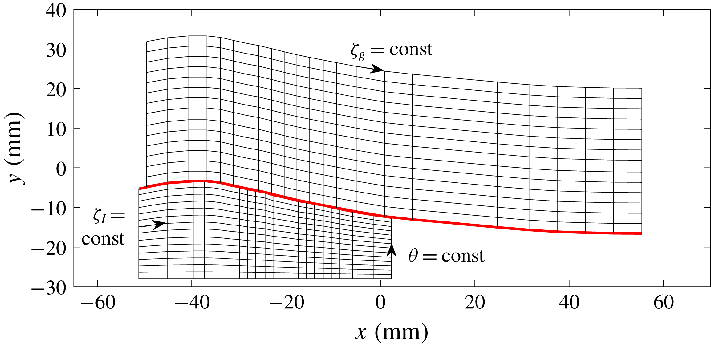
The wave-following coordinate system applied is illustrated in figure 14. The wave phase
 $\unicode[STIX]{x1D703}$
(evaluated by the zero-crossing procedure described in § 3.2) is used together with a wave-following
 $\unicode[STIX]{x1D701}$
-coordinate to obtain a wave-following coordinate system. The
 $\unicode[STIX]{x1D701}$
-coordinate is implemented slightly differently in the two phases. In the liquid phase,
 $\unicode[STIX]{x1D701}_{l}$
is evenly distributed over 100 points from the lower part of the PIV velocity field (at
 $y=-28$
mm) to the interface. This is similar to the wave-following coordinate system applied by Vollestad et al. (Reference Vollestad, Ayati and Jensen2019b
). In the gas phase the wave amplitude is a critical parameter, impacting on the extent of the sheltered region. For this reason the
 $\unicode[STIX]{x1D701}_{g}$
-coordinate is normalized by the wave crest height;
 $\unicode[STIX]{x1D701}_{g}$
is evenly distributed over 100 points, from the interface to a height
 $5\times y_{max}$
above the interface. This ensures that points in the trough-to-crest region are sampled at the same relative height above the interface, ensuring a more physical phase-averaged value in this region. This coordinate system is similar to the coordinate system applied by Vollestad et al. (Reference Vollestad, Ayati, Angheluta, LaCasce and Jensen2019a
), evaluating the phase-averaged properties of airflow above waves.
Example coordinate system. Only a small fraction of the gridlines included. Red line: interface.

The horizontal and vertical velocity components of breaking and non-breaking waves are sampled individually, and averaged at constant
 $(\unicode[STIX]{x1D703},\unicode[STIX]{x1D701})$
-coordinates to obtain the phase-averaged velocities
 $\langle u\rangle$
and
 $\langle v\rangle$
. When performing the averaging, the average interface elevation (based on the LFV camera) is also evaluated. When presenting the phase-averaged results the (
 $\unicode[STIX]{x1D703},\unicode[STIX]{x1D701}$
)-coordinates are transformed into (
 $\unicode[STIX]{x1D703},y$
)- or (
 $x,y$
)-coordinates (depending on the application) based on the mean interface.