


Introduction
Theoretical treatments of continental ice sheets concentrate on the dynamics of the problem and are primarily concerned with explaining the climatic variations of ice volume and extent (e.g. Reference WeertmanWeertman, 1964, Reference Weertman1976; Reference BirchfieldBirchfield, 1977; Reference Watts and Hayder.Watts and Hayder, 1983). The more complex of them are fully fledged three-dimensional numerical models which take into account both the dynamics and thermodynamics of the medium, and to some extent also such things as bedrock depression and the detail of the ice-edge interaction with the surrounding ocean (e.g. Reference Birchfield, Weertman and Lunde.Birchfield and others. 1981; Reference PollardPollard, 1982; Reference Budd. and Jenssen.Budd and Jenssen, 1989; Reference HuybrechtsHuybrechts, 1991). Perhaps their major success has been simulation of the ice-volume changes which, at least during the Quaternary, contain cyclical components on time-scales of 20, 40 and 100 ka. They provide an explanation of these cycles in terms of variations of solar input induced by orbital changes of the Earth, i.e. in terms of Milankovitch forcing.
In the present paper, a simple and semi-qualitative steady-state mass and energy-balance model of the Antarctic ice sheet is used to derive order-of-magnitude sensitivities to such things as ground heal flux. It is used also as a vehicle to illustrate the possible importance of changes in ground heat flux induced by convection of water in the underlying crust.
The Steady-State Model
Imagine an idealized ice sheet which completely covers its underlying continent. The continent is surrounded by deep ocean, and has a horizontal radius R and a bedrock surface roughness of vertical scale L. The rate a of accumulation (precipitation minus evaporation) is constant across its surface and is balanced by ablation (calving or melting) at the ice-sheet edge when the system is in steady state. Mass continuity requires that

where v(r) is the vertically averaged deformation velocity at radius r, and Z(r) is the height of the ice at that radius. Glen’s law relating strain rate to stress gives an expression for deformation velocity as a function of height and of the gradient of height, namely
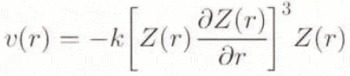
where k is a constant related to the fluidity of the medium. Under the assumption that a(r) is constant across the surface, Equation (1) can be integrated to yield an expression for the central height H as

The theoretical shape of such a steady-state ice sheet is parabolic. It has an average height h which is not much less than the central height H. For simplicity, in the following we assume a flat-topped ice sheet of height h, with much the same functional relation of height to accumulation rate as in Equation (3), namely

where A 0 is a constant which does not change provided that the fluidity k of the ice does not change. Its numerical value (chosen here to match present-day values of height and accumulation rate) is 1.73 × 10⁴ in units of m/(kg m−2 s−1)⅛. The accumulation rate is specifically written as a function of height in Equation (4), namely as a(h). The function is quoted in the caption to Figure 1, and is such that a(h) is a constant a 0 for the first kilometer (a 0 is equivalent to 60 cm year−1) and decreases exponentially with height above 1 km. At 3.5 km for instance, the rate is equivalent to 15 cm year−1.
Steady-state ice-sheet height h (solid lines) and potential basal temperature T b, (dashed lines) as a function of ground heat flux q for various values of sea-level temperature T sl. The boundary conditions are the relevant “standard” values as in the second row of Table 1. The vertical profile of accumulation rate is a constant a 0 for the first 1000 m, and decreases above 1000 m according to a(h) = a 0 exp [−0.693(h –1000)].

The effective value of k will change if the basal temperature T b exceeds the pressure-melting temperature T 0 and there is water at the bottom of the ice. For the purpose of the present paper, imagine that T b is a “potential” basal temperature, i.e. the basal temperature that would pertain if by some means the ice were not allowed to melt. Thus T b is the actual basal temperature if T b < T 0 (when there is no water at the base and when Equation (4) applies) but is a theoretical temperature greater than T 0 when there is water at the base. Imagine further that it is possible for the water at the base of the ice to have significant depth D above the deepest points of the bedrock and that D is an increasing function of T b – T 0. For instance, if the ground heat flux is enough to start melting ice. then the greater is the heat flux, the greater is T b – T 0, the greater is the volume of water at the base, and the faster slides the ice. This naive picture is used as a “construct” on which to develop a functional relation between h and T b (and ultimately between h and ground heat flux) for the case when there is water at the base of the ice.
Thus it is assumed that when basal water is present the average height h of the ice is reduced below the value given by Equation (4) in proportion to the water volume. If one imagines “lakes” of water beneath the ice in the valleys between the roughness elements of the bedrock, and imagines further that there is no connection allowing water to flow between the lakes or between the lakes and the surrounding ocean, then one is led to a modification of Equation (4) as follows:

where D (the “depth” of the lakes) and L (the height of the roughness elements) are measured with reference to the lowest points of the bedrock surface, and where h is now the ice-sheet height above the surface of the water. This rather arbitrary linear modification of Equation (4) assumes that when there is sufficient water to cover the roughness elements of the bedrock surface (i.e. when D = L) the overall ice sheet will flow or slide sufficiently fast to reduce the steady-state height to zero.
The primary objection to this physical picture is the assumption that the water beneath the ice is not connected to the ocean and can therefore build up into lakes of significant depth. The objection is certainly valid, but on the other hand there is evidence for the existence of such lakes, and some of them (the recently discovered Lake Vostok, for instance) are very extensive. In any event, the picture is simply a means of suggesting a function governing the reduction in steady-state height with increasing water volume, recognizing that the water volume in turn will be determined by T b (see Equation (6) below). The picture itself is not greatly important to the argument other than that it emphasizes the problems of quantitative analysis at this level of simplicity.
At a similar level of approximation, the actual value of steady-state water depth D is assumed to be some fraction of h determined by the difference between potential basal temperature and the pressure-melting temperature. That is,

where T 1 is the average temperature at the top of the ice.
In summary of this point. Equation (4) determines the ice-sheet height when T b < T 0 and there is no water at the base, and Equations (5) and (6) determine ice-sheet height when T b > T b and the base is wet.
In order to establish a second relation between h and T b, consider the overall energy balance of the steady-state ice sheet as a whole. The inputs of energy are ground heat flux q, the rate of input of potential energy a(h)gh corresponding to the accumulation of mass at the top of the ice sheet (g is the acceleration due to gravity), and the rate of input of heat into the ice a(h)c p T 1 associated with the accumulation of mass at temperature T 1. c p is the heat capacity of ice. T 1 is the boundary temperature at the top of the ice sheet, maintained by various ice/air energy exchange processes at that height and governed by sea-level temperature T sl via the atmospheric lapse rate A. That is, T 1 = T sl – Ah. The potential energy associated with mass accumulation is converted to heat within the ice sheet via the basal friction or deformation of the flowing ice. An approximate energy-balance equation with the inputs on the lefthand side is as follows:

There are two output terms on the righthand side. It is assumed with regard to them, again simply for the sake of convenience rather than reality, that the vertical profile of temperature in the ice is linear. By this means the potential basal temperature T b, can be incorporated easily in the equation via both of the energy output terms. The first such term is the rate of upward conduction of heat to the ice-sheet surface through ice of thermal conductivity b. The second is the rate of heat loss of the system associated with the ablation at the ice-sheet edge. The ablation is assumed to occur at a temperature equal to the average of the top and basal temperatures.
The conduction term might be regarded as a proxy for the net heat exchange away from the upper surface of the ice via radiation and turbulence. If there were no upward heat conduction, the net radiative and turbulent exchange would be zero. If there is a vertical temperature gradient in the ice (and the present picture assumes a linear gradient from the bottom to the top of the ice), then there must be a net flux of heat out of the top which is “carried away” by the net radiative and turbulent transfer. In such a case, the net balance at the surface includes the upward conduction of heat, but must still be zero overall. All of which ignores the deposition of heat associated with the mass accumulation at temperature T 1 (the third input term on the lefthand side of Equation (7)). That deposition is separated out from the above discussion of the net flux at the top of the ice because it does not affect the maintenance of the boundary temperature T 1. In any event, there is a corresponding heat-loss term (associated with the loss of mass at the edges of the ice sheet; and in steady state the mass is lost at the same rate as the accumulation) on the righthand side. The mass is lost at some temperature between T 1 and the basal temperature T b, and for the sake of argument that temperature is simply taken as the average of T 1 and T b.
If sea-level temperature, atmospheric lapse rate and the ground heat flux are specified as boundary conditions, and if the accumulation rate a(h) is specified as a function of height (as in the caption to Figure 1 for example), Equations (5) and (7) can be solved for the potential basal temperature T b and the average height h. The relevant equations are Equations (4) and (7) for the case where T b < T 0 and there is no water at the base of the ice. Note that the equations as formulated cannot be applied when the ice-sheet height is less than the vertical scale of the roughness elements of the bedrock.
Steady-State Behaviour
Figure 1 gives h and T b, as a function of basal heat flux q for the set of “standard” boundary conditions mentioned in the caption. It makes the point that when the base is dry (T b is less than T 0) the ice-sheet height and volume are independent of q, since h is determined only by Equation (4). When there is water at the base, increasing q increases the volume of the water and decreases the steady-state height. At the value of q labelled as “standard” in Figure 1 (0.063 W m−2 is the normally quoted figure for the average ground heat flux of continents in general, although Reference DrewryDrewry (1979) reports a slightly higher value from specific measurements in Antarctica) the input of potential energy from the falling snow is almost exactly equal to q. It is worth noting the somewhat counter-intuitive result that T b decreases as h increases. This is because both the precipitation (and hence the potential energy input) and the upper- boundary temperature decrease with height. It seems that the basal temperature of an ice sheet will always be within a few degrees of the pressure-melting temperature, and water is more likely to be found under thinner rather than thicker ice sheets.
The sensitivity of h and T b to change in the boundary conditions depends on the position of the ice sheet in the “space” of those conditions, Table 1 gives sensitivities (i.e. partial derivatives) calculated at a position defined by the “standard” values in row 2 of the table. The model is least sensitive to the scale of the surface roughness of the underlying continent, It is highly sensitive to sea-level temperature T sl, which is something of a problem since this parameter is perhaps the most arbitrary of the various selections of boundary condition. T sl is intended to represent the sea-level temperature that would exist at the surface of the continent if the ice sheet were removed, and as a first approximation was chosen here to be much the same as the observed mean annual temperature of the North Pole, whose elevation is close to zero.
Partial derivatives of ice-sheet steady-state h and T bwith respect to each of the external parameters x at the “standard” values of the parameters as shown in the second row. Values were calculated numerically simply by making small alterations to the parameters one at a time. Units of h in meters, of Tbin °C. The rows of partial derivatives multiplied by the standard parameter value are an attempt to put the changes on a comparable footing, i.e. of doubling the absolute values of the parameters. “Doubling” temperature means very little in this context, and the relevant entries are labelled “n/a”

Various models suggest that a likely scenario of climate change arising from enhanced greenhouse warming would be an increase of sea-level temperature together with an increase of precipitation. Figure 2 is a graph of h as a function of simultaneously varying T sl and a as indicated by the dual x-axis scales in the figure. The scales assume that accumulation rate increases about 5% for every degree of increased sea-level temperature. There is a broad maximum in the curve. At lower temperatures and accumulation rates, h increases with a according to Equation (4) since there is no basal water. At higher temperatures and accumulation rates, the effect of T sl dominates via its control of basal temperature and basal water, and h decreases as T sl increases. If one accepts the various approximations and assumptions of the model, the present “position” of the Antarctic ice sheet may not be too far from the maximum of the curve. Put another way, if the Earth’s climate were to change according to a typical enhanced-greenhouse scenario, one would not (according to this model) expect a large change in the volume of the Antarctic ice. The conclusion assumes among other things that the dynamic response to any imposed change of boundary condition is a reasonably smooth move towards the new steady state: that the intermediate changes on the way to the new steady state are not greater than the difference between initial and final steady states.
Variation of steady-state height h with simultaneous variation of sea-level temperature and accumulation rate as indicated on the x axis.

Ground Heat Flux and Dynamical Behaviour
It is known that the vertical heat flux through the Earth’s crust can change on the time-scale of millions or years. It is believed that in certain circumstances it can change by almost an order of magnitude on shorter time-scales because of convection of water (and consequently of heat) within the uppermost few kilometers of crust. The concept of crustal water convection has been built into models of the deep ocean floor (Reference CathlesCathles, 1990; Reference Rosenberg, Spera and Haymon.Rosenberg and others, 1993) and into models of the behaviour of thermally active regions of the continents (Reference DonaldsonDonaldson, 1962).
If one accepts that the Antarctic ice sheet has (or has had in the past) water at its base, it is not too much of an extension to assume that the underlying continental crust is effectively water-saturated. (One might argue that the process of saturation would he aided by fracturing associated with ice-sheet loading.) Having gone that far, it is of interest to examine the possible consequences of changes in ground heat flux associated with water convection.
Imagine the underlying crust has a lower-boundary temperature of 1300°C at a depth of about 35 km. Upward heat transfer is by conduction, and if the conductivity is constant and the system is in steady state there will be a linear temperature gradient dT/dz throughout the entire depth. Imagine there is a water-saturated layer in the uppermost 3 km where the temperature is less than about 350°C. (At higher temperatures the crust is sufficiently “fluid” to close off the pores and channels which allow the convection of water.) For the water to convert, the Rayleigh number Rn (Rn is an increasing function of the vertical temperature gradient) must exceed a certain critical value R n1. Once convection takes place, the effective conductivity of the layer increases. There is a corresponding increase in q, which in turn drains heat from the upper layer and lowers its temperature gradient. Ultimately the gradient becomes low enough to reduce Rn below a critical value R n2 (not necessarily equal to R n1 because of hysteresis), and the layer conductivity returns to its non-convective value. There is therefore a possible cyclical variation of q, with a cycle time determined by the heat capacity of the upper layer and the difference between the temperature gradients which determine the onset and offset of convection. The convective heat flux may be an order of magnitude greater than that of conduction.
Figure 3 gives the time-dependent variation of h and q obtained by combining the ice-sheet equations above with a numerical solution of the time-dependent heat-conduction equation applied to a continental crust behaving in the manner just described. The details of the calculations are given in the caption. The steady-state ice-sheet equations were converted to an effective time-dependent model by the simple expedient of assuming that, when q changes at any time step, the ice sheet will exponentially relax towards the new steady state corresponding to the new q with a time-constant (in this example) of 20 000 years.
Time variation of ground heat flux q (solid curve) from a time-dependent numerical one-dimensional crustal model of 100 layers each 350 m thick (see text). The crust has a specific heat of 800 J kg−1 °C−1 and a conductivity of 1.3 W m− °C−1. The switch to an effective conductivity ten times this value for the upper ten layers occurs when the average temperature gradient of those layers exceeds 0.030°C m−1, and returns to the lower value when the gradient is less than 0.026°C m−1. The initial condition is a linear temperature gradient from the top (at 0°C) to the bottom (at 1300°C). The time step is 100 years. The output q is used to drive an ice-sheet “model” which continually relaxes toward the potential steady-state value of h corresponding to the instantaneous value of q. The relaxation time constant is 20 ka. The dashed curve is the calculated variation of h.

The figure is a qualitative illustration of a possible consequence of what might be one mechanism for introducing cyclical behaviour on climatic time-scales into extensive continental ice sheets. In this illustration the parameters of the crust, and in particular the effective values of critical temperature gradient, have been deliberately and arbitrarily chosen to yield a cycle time of about 100 000 years, which is a dominant cycle associated with polar ice sheets over the Quaternary.



