1 Introduction
An important aspect of many international CO2 emissions reduction plans involves storing CO2 within the pore space of brine-containing aquifers, often referred to as saline formations (Nordbotten & Celia Reference Nordbotten and Celia2006; MacMinn, Szulczewski & Juanes Reference MacMinn, Szulczewski and Juanes2010). The reason for choosing saline formations as opposed to freshwater aquifers is the idea that brine is sufficiently saline that it is unlikely to be suitable for exploitation as a future water resource. However, the dissolved salt within the brine can lead to operational problems (Miri & Hellevang Reference Miri and Hellevang2016).
When CO2 is injected into a saline formation, there is a high interfacial area between the CO2 and the brine. Consequently, there is dissolution of CO2 into the brine and evaporation of the water into the CO2-rich phase (Spycher, Pruess & Ennis-King Reference Spycher, Pruess and Ennis-King2003). Surrounding the injection well, a dry-out zone develops where the water in the brine is completely evaporated. A consequence of this evaporation is that the dissolved salt precipitates as a solid phase, leading to significant loss of permeability around the injection well. Ultimately, this process can lead to complete deterioration of the injection well (Miri & Hellevang Reference Miri and Hellevang2016).
A number of numerical modelling studies have been undertaken to investigate important controls on salt precipitation in the dry-out zone. Zeidouni, Pooladi-Darvish & Keith (Reference Zeidouni, Pooladi-Darvish and Keith2009) derived an analytical solution using method of characteristics (MOC) to estimate the volume fraction of precipitated salt in the dry-out zone (hereafter referred to as
 $C_{30}$
) due to CO2 injection in saline formations. They concluded that the distribution of precipitated salt was uniform within the dry-out zone.
An important limiting assumption was that there is a local pressure equilibrium between the CO2-rich and aqueous phases. The difference between the pressures of a non-wetting and wetting phase (the CO2-rich and aqueous phases, respectively, in this context) is referred to as the capillary pressure. Pruess & Muller (Reference Pruess and Muller2009) explored the same problem using the numerical reservoir simulator, TOUGH2, with the CO2 storage module, ECO2N (Pruess & Spycher Reference Pruess and Spycher2007). When capillary pressure is set to zero,
 $C_{30}$
is found to be insensitive to injection rate. However, when capillary pressure is accounted for,
 $C_{30}$
is found to increase with reducing CO2 injection rate.
A physical explanation is provided as follows (Pruess & Muller Reference Pruess and Muller2009): capillary pressure is significantly increased as the wetting saturation is reduced. This can lead to a reversing in the direction of the wetting pressure gradient, which in turn results in counter-current flow, whereby brine flows in the opposite direction to the injected CO2. The counter-current flow provides additional brine to the dry-out zone leading to an increased availability of salt for precipitation. The counter-current flow rate is driven by phase saturation gradients. As the injection rate increases, the counter-current flow becomes less significant in comparison.
Kim et al. (Reference Kim, Han, Oh, Kim and Kim2012) extended the work of Pruess & Muller (Reference Pruess and Muller2009) by performing a wider sensitivity analysis. They found that the value of
 $C_{30}$
was significantly increased for scenarios involving high permeability and low injection rates. Furthermore, contrary to Zeidouni et al. (Reference Zeidouni, Pooladi-Darvish and Keith2009), they found that
 $C_{30}$
was non-uniform, with the highest values present at the edge of the dry-out zone. This localized increase in salt precipitation is attributed to the combined effects of gravity and capillary pressure driven counter-current flow.
Li, Tchelepi & Benson (Reference Li, Tchelepi and Benson2013) found that smoother capillary pressure curves lead to faster dissolution of CO2 into the aqueous phase. This is presumably because smoother capillary pressure curves lead to more capillary diffusion of the CO2-rich phase and hence greater interfacial area between the CO2-rich phase and the aqueous phase.
The suite of numerical simulations described by Pruess & Muller (Reference Pruess and Muller2009) and Kim et al. (Reference Kim, Han, Oh, Kim and Kim2012) have provided significant insight into the processes that control salt precipitation during CO2 injection in saline formations. However, probably due to the perceived computational expense of numerically simulating this problem to an adequate accuracy, a more widespread sensitivity analysis has not been undertaken to further understand this process.
Analytical solutions have been developed to better understand many other aspects of the CO2 storage process. Nordbotten & Celia (Reference Nordbotten and Celia2006) developed a similarity solution to study the propagation rate of a CO2 plume and its associated dry-out zone during injection of CO2 into a cylindrical saline formation. Hesse et al. (Reference Hesse, Tchelepi, Cantwell and Orr2007), Hesse, Orr & Tchelepi (Reference Hesse, Orr and Tchelepi2008) and MacMinn et al. (Reference MacMinn, Szulczewski and Juanes2010), MacMinn, Szulczewski & Juanes (Reference MacMinn, Szulczewski and Juanes2011) developed MOC solutions to study the migration of CO2 plumes following the cessation of injection. Mathias et al. (Reference Mathias, Gonzalez Martinez de Miguel, Thatcher and Zimmerman2011a ) extended the analytical solution of Nordbotten & Celia (Reference Nordbotten and Celia2006) to estimate the resulting pressure buildup within an injection well. Mathias et al. (Reference Mathias, Gluyas, Gonzlez Martnez de Miguel and Hosseini2011b ) combined the work of Zeidouni et al. (Reference Zeidouni, Pooladi-Darvish and Keith2009) and Mathias et al. (Reference Mathias, Gonzalez Martinez de Miguel, Thatcher and Zimmerman2011a ) to study the role of partial miscibility between the CO2 and brine on pressure buildup. More recently, Mathias, McElwaine & Gluyas (Reference Mathias, McElwaine and Gluyas2014) derived a MOC solution to estimate the temperature distribution around a CO2 injection in a depleted gas reservoir. There are many other such examples in the literature. However, all the analytical solutions presented to date revolve around the CO2 transport problem reducing to a hyperbolic partial differential equation (PDE), such that MOC or some variant can be used for the solution procedure. The difficulty of accounting for capillary pressure is that this leads to a diffusive component within the equations, rendering MOC inadequate in this regard.
Unrelated to CO2 storage, McWhorter & Sunada (Reference McWhorter and Sunada1990) derived a similarity solution to look at two-phase immiscible flow around an injection well, which explicitly captures the counter-current flow associated with capillary pressure effects. In the past, their solution has not been commonly used due to difficulties with evaluating the necessary nonlinear multiple integrals associated with their equations (Fucik et al. Reference Fucik, Mikyska, Benes and Illangasekare2007). However, more recently, Bjornara & Mathias (Reference Bjornara and Mathias2013) have provided a more efficient evaluation procedure by re-casting the equations as a boundary value problem, which they then solve using a Chebyshev polynomial differentiation matrix (Weideman & Reddy Reference Weideman and Reddy2000).
The objective of this study is to use the method of Bjornara & Mathias (Reference Bjornara and Mathias2013) and extend the similarity solution of McWhorter & Sunada (Reference McWhorter and Sunada1990) to account for partial miscibility of phases, so as to study the control of capillary pressure on salt precipitation during CO2 injection in saline formations.
The outline of this article is as follows. First, a PDE to describe partially miscible three-phase flow is presented. This is then reduced to an ordinary differential equation (ODE) by application of a similarity transform. The resulting boundary value problem is solved using a Chebyshev polynomial differentiation matrix. The necessary equations are then presented to determine the volume fraction of precipitated salt in the dry-out zone. A set of verification examples are presented based on a gas-displacing-oil scenario, previously presented by Orr (Reference Orr2007). A CO2-injection-in-a-saline-formation scenario is then presented, which is compared with simulation results from TOUGH2 for verification. Finally, a wider sensitivity analysis is conducted to better understand the main controls in this context.
2 Mathematical model
A homogenous, cylindrical and porous saline formation is invoked with a thickness of
 $H$
[L] and an infinite radial extent. The pore space is initially fully saturated with a brine of uniform NaCl concentration. Pure CO2 is injected at a constant rate of
 $Q_{0}$
[L3T-1] into the centre of the saline formation via a fully penetrating injection well of infinitesimally small radius. The permeability of the saline formation is horizontally isotropic. However, a necessary simplifying assumption is that the vertical permeability is significantly smaller than the horizontal permeability such that gravity effects can be neglected. In this way, during the injection phase, fluid flow can be treated as a one-dimensional radially symmetric process.
Now we will describe the material mixture that resides within the pore space. Consider a mixture of three components:
 $i=1,2$
and 3. Components 1 and 2 are mutually soluble and can reside within both a non-wetting fluid phase and a wetting fluid phase, denoted hereafter as
 $j=1$
and 2, respectively. Component 3 can dissolve into phase 2 and precipitate to form a solid phase, denoted hereafter as
 $j=3$
. However, component 3 is assumed not to be able to reside in phase 1 and components 1 and 2 are assumed not to be able to reside in phase 3. In the context of a CO2–H2O–NaCl system,
 $i=1,2$
and 3 for CO2, H2O and NaCl, respectively. All components are assumed to be incompressible and not to experience volume change on mixing, such that component densities can be treated as constant throughout.
The volume fraction of component
 $i$
for the combined mixture,
 $C_{i}$
[-], is defined by
 $$\begin{eqnarray}C_{i}=\mathop{\sum }_{j=1}^{3}\unicode[STIX]{x1D70E}_{ij}S_{j},\end{eqnarray}$$
where
 $\unicode[STIX]{x1D70E}_{ij}$
[-] is the volume fraction of component
 $i$
in phase
 $j$
and
 $S_{j}$
[-] is the volume fraction of phase
 $j$
for the combined mixture, often to referred to as the saturation of phase
 $j$
.
With no additional assumptions, it can be said that
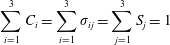 $$\begin{eqnarray}\mathop{\sum }_{i=1}^{3}C_{i}=\mathop{\sum }_{i=1}^{3}\unicode[STIX]{x1D70E}_{ij}=\mathop{\sum }_{j=1}^{3}S_{j}=1\end{eqnarray}$$
and
 $$\begin{eqnarray}\unicode[STIX]{x1D70E}_{ij}=\left\{\begin{array}{@{}llll@{}}C_{i}, & C_{1}\notin (c_{12}(1-S_{3}),c_{11}(1-S_{3})), & i\in \{1,2\}, & j\in \{1,2\}\\ c_{ij}, & C_{1}\in (c_{12}(1-S_{3}),c_{11}(1-S_{3})), & i\in \{1,2\}, & j\in \{1,2\}\\ 0, & C_{1}\in [0,1], & i\in \{1,2\}, & j=3\\ 0, & C_{3}\in [0,1], & i=3, & j=1\\ C_{3}/S_{2}, & C_{3}\in [0,c_{32}S_{2}), & i=3, & j=2\\ c_{32}, & C_{3}\in [c_{32}S_{2},1], & i=3, & j=2\\ 1, & C_{3}\in [0,1], & i=3, & j=3,\end{array}\right.\end{eqnarray}$$
where
 $c_{ij}$
[-] is the constant equilibrium volume fraction of component
 $i$
in phase
 $j$
. It further follows that
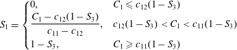 $$\begin{eqnarray}S_{1}=\left\{\begin{array}{@{}ll@{}}0, & C_{1}\leqslant c_{12}(1-S_{3})\\ \displaystyle \frac{C_{1}-c_{12}(1-S_{3})}{c_{11}-c_{12}}, & c_{12}(1-S_{3})<C_{1}<c_{11}(1-S_{3})\\ 1-S_{3}, & C_{1}\geqslant c_{11}(1-S_{3})\end{array}\right.\end{eqnarray}$$
and
 $$\begin{eqnarray}S_{3}=\left\{\begin{array}{@{}lll@{}}0, & 0\leqslant C_{1}\leqslant 1, & C_{3}<c_{32}S_{2}\\ \displaystyle \frac{C_{3}-c_{32}}{1-c_{32}}, & C_{1}\leqslant c_{12}(1-S_{3}), & C_{3}\geqslant c_{32}S_{2}\\ \displaystyle \frac{(c_{11}-c_{12})C_{3}-(c_{11}-C_{1})c_{32}}{(1-c_{32})c_{11}-c_{12}}, & c_{12}(1-S_{3})<C_{1}<c_{11}(1-S_{3}), & C_{3}\geqslant c_{32}S_{2}\\ C_{3}, & C_{1}\geqslant c_{11}(1-S_{3}), & C_{3}\geqslant c_{32}S_{2}.\end{array}\right.\end{eqnarray}$$
Under the above set of assumptions, fluid flow is controlled by the following set of one-dimensional radially symmetric mass conservation equations
 $$\begin{eqnarray}\unicode[STIX]{x1D719}\frac{\unicode[STIX]{x2202}C_{i}}{\unicode[STIX]{x2202}t}=-\frac{1}{r}\frac{\unicode[STIX]{x2202}}{\unicode[STIX]{x2202}r}\left(r\mathop{\sum }_{j=1}^{2}q_{j}\unicode[STIX]{x1D70E}_{ij}\right),\quad i\in \{1,2,3\},\end{eqnarray}$$
where
 $\unicode[STIX]{x1D719}$
[-] is the saline formation porosity,
 $t$
[T] is time,
 $r$
[L] is radial distance from the injection well and
 $q_{j}$
[LT-1] is the flow of phase
 $j$
per unit area, which can be found from Darcy’s law
 $$\begin{eqnarray}q_{j}=-\frac{kk_{rj}}{\unicode[STIX]{x1D707}_{j}}\frac{\unicode[STIX]{x2202}P_{j}}{\unicode[STIX]{x2202}r},\quad j\in \{1,2\},\end{eqnarray}$$
where
 $k$
[L2] is the saline formation permeability and
 $k_{rj}$
[-],
 $\unicode[STIX]{x1D707}_{j}$
[ML-1T-1] and
 $P_{j}$
[ML-1T-2] are the relative permeability, dynamic viscosity and pressure of phase
 $j$
, respectively.
A detailed discussion with regards to justification for the above set of assumptions is provided in § 4 below.
The difference between the non-wetting and wetting phase pressure is referred to as the capillary pressure,
 $P_{c}$
[ML-1T-2], i.e.
 $$\begin{eqnarray}P_{c}=P_{1}-P_{2}.\end{eqnarray}$$
Because the component densities are assumed to be constant, the system of equations is divergence free and
 $$\begin{eqnarray}\mathop{\sum }_{j=1}^{2}q_{j}=\frac{Q_{0}}{2\unicode[STIX]{x03C0}Hr}.\end{eqnarray}$$
Substituting (2.7) and (2.8) into (2.9), solving for the partial derivatives of
 $P_{j}$
and then substituting these back into (2.7) leads to
 $$\begin{eqnarray}q_{j}=\frac{Q_{0}\,f_{j}}{2\unicode[STIX]{x03C0}Hr}+\frac{(-1)^{j}kk_{r1}\,f_{2}}{\unicode[STIX]{x1D707}_{1}}\frac{\unicode[STIX]{x2202}P_{c}}{\unicode[STIX]{x2202}r},\end{eqnarray}$$
where, with further consideration of (2.4),
 $$\begin{eqnarray}f_{j}=\left\{\begin{array}{@{}ll@{}}[1+(-1)^{j}]/2, & C_{1}\leqslant c_{12}(1-S_{3})\\ \displaystyle \frac{k_{rj}}{\unicode[STIX]{x1D707}_{j}}\left(\mathop{\sum }_{j=1}^{2}\frac{k_{rj}}{\unicode[STIX]{x1D707}_{j}}\right)^{-1}, & c_{12}(1-S_{3})<C_{1}<c_{11}(1-S_{3})\\ \text{}[1+(-1)^{j-1}]/2, & C_{1}\geqslant c_{11}(1-S_{3}).\end{array}\right.\end{eqnarray}$$
Also note that there is no capillary pressure gradient when only one fluid phase is present, i.e.
 $$\begin{eqnarray}\frac{\unicode[STIX]{x2202}P_{c}}{\unicode[STIX]{x2202}r}=0,\quad C_{1}\notin (c_{12}(1-S_{3}),c_{11}(1-S_{3})).\end{eqnarray}$$
Substituting (2.10) into (2.6), therefore leads to
 $$\begin{eqnarray}\frac{\unicode[STIX]{x2202}C_{i}}{\unicode[STIX]{x2202}\unicode[STIX]{x1D70F}}=-\frac{\unicode[STIX]{x2202}F_{i}}{\unicode[STIX]{x2202}\unicode[STIX]{x1D709}},\end{eqnarray}$$
where
 $$\begin{eqnarray}F_{i}=\left\{\begin{array}{@{}ll@{}}\unicode[STIX]{x1D70E}_{i2}, & C_{1}\leqslant c_{12}(1-S_{3})\\ \displaystyle \mathop{\sum }_{j=1}^{2}f_{j}\unicode[STIX]{x1D70E}_{ij}+\left(\frac{k_{r1}\,f_{2}}{Ca}\mathop{\sum }_{j=1}^{2}(-1)^{j}\unicode[STIX]{x1D70E}_{ij}\right)\unicode[STIX]{x1D709}\frac{\unicode[STIX]{x2202}\unicode[STIX]{x1D713}}{\unicode[STIX]{x2202}\unicode[STIX]{x1D709}}, & c_{12}(1-S_{3})<C_{1}<c_{11}(1-S_{3})\\ \unicode[STIX]{x1D70E}_{i1}, & C_{1}\geqslant c_{11}(1-S_{3})\end{array}\right.\end{eqnarray}$$
and
 $$\begin{eqnarray}\displaystyle & \unicode[STIX]{x1D70F}={\displaystyle \frac{Q_{0}t}{\unicode[STIX]{x03C0}\unicode[STIX]{x1D719}Hr_{e}^{2}}}, & \displaystyle\end{eqnarray}$$
 $$\begin{eqnarray}\displaystyle & \displaystyle \unicode[STIX]{x1D709}=\frac{r^{2}}{r_{e}^{2}}, & \displaystyle\end{eqnarray}$$
 $$\begin{eqnarray}\displaystyle & \displaystyle \unicode[STIX]{x1D713}=\frac{P_{c}}{P_{c0}}, & \displaystyle\end{eqnarray}$$
where
 $r_{e}$
[L] is an arbitrary reference length,
 $P_{c0}$
[ML-1T-2] is a reference ‘air-entry’ pressure for the porous medium of concern and
 $Ca$
[-] is a dimensionless constant often referred to as the capillary number, found from
 $$\begin{eqnarray}Ca=\frac{Q_{0}\unicode[STIX]{x1D707}_{1}}{4\unicode[STIX]{x03C0}HkP_{c0}}.\end{eqnarray}$$
The capillary number represents the ratio of the CO2 injection rate to the product of the CO2 mobility and air-entry pressure of the porous medium. It compares the relative effect of the frictional resistance associated with fluid movement with the surface tension, which acts across the interface between the CO2-rich phase and the aqueous phase. Small values of
 $Ca$
imply that capillary processes are important.
With regards to the initial condition and boundary conditions, let
 $C_{iI}$
[-] represent a uniform initial value of
 $C_{i}$
in the saline formation and
 $C_{i0}$
[-] represent a constant boundary value of
 $C_{i}$
at the injection well for
 $i\in \{1,2,3\}$
.
2.1 Writing capillary pressure in terms of
 $C_{1}$

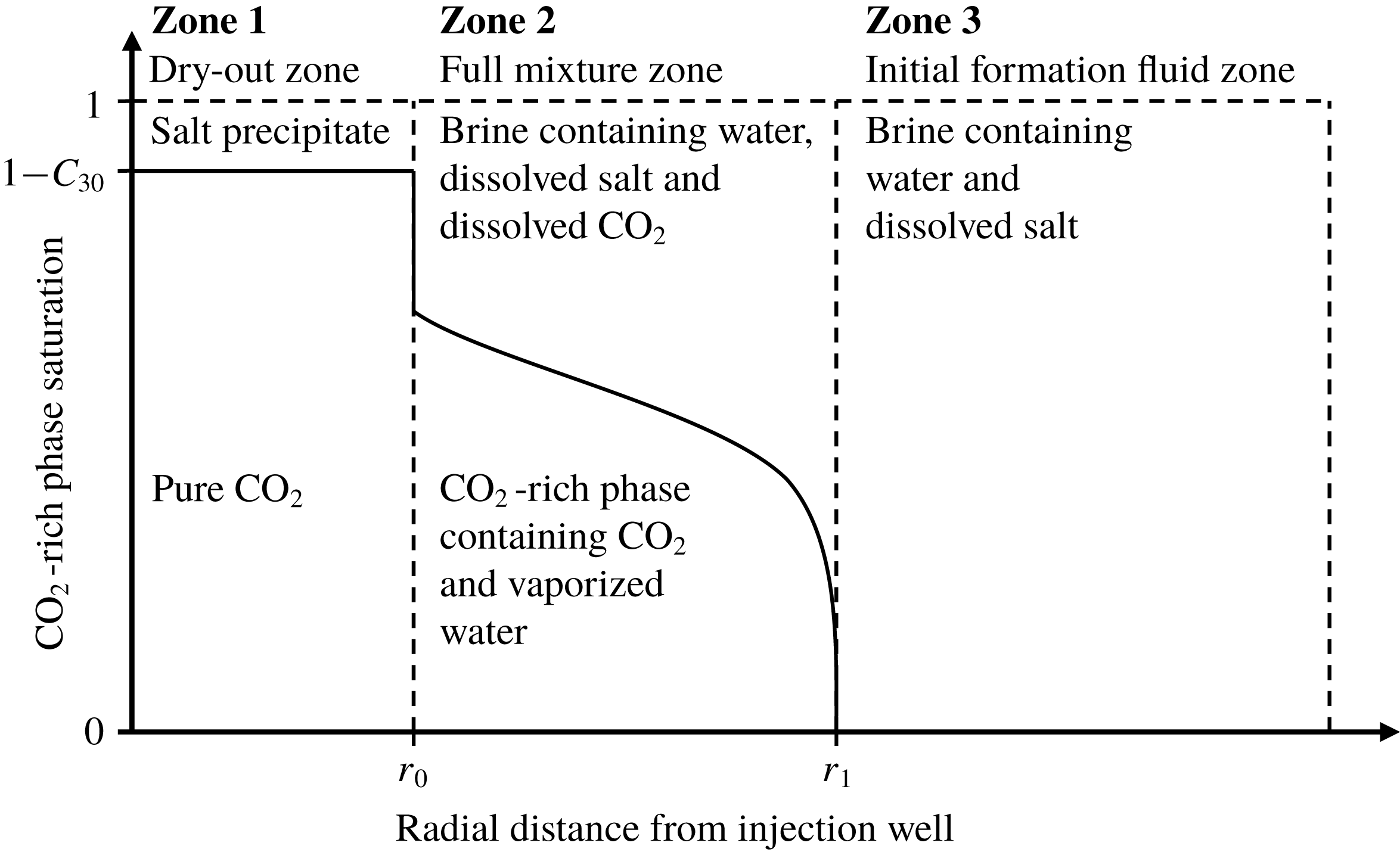
As CO2 is injected into the saline formation, H2O evaporates from the brine leaving NaCl behind as a precipitate in a dry-out zone that develops around the injection well. Following the commencement of CO2 injection, there are therefore three distinct zones within the saline formation that should be considered (see figure 1): (i) The dry-out zone, which surrounds the injection well and contains only precipitated salt and CO2 in the non-wetting fluid phase. (ii) The full mixture zone, which surrounds the dry-out zone and contains CO2, H2O and NaCl, distributed between the wetting and non-wetting fluid phases. (iii) The initial saline formation fluid zone, which surrounds the full mixture zone and contains only H2O and NaCl in a wetting fluid phase.
A schematic diagram illustrating the distribution of CO2, water and salt around a CO2 injection well in a saline formation.

Inspection of (2.13) and (2.14) reveals that the problem is hyperbolic for
 $C_{1}\notin (c_{12}(1-S_{3}),c_{11}(1-S_{3}))$
and not hyperbolic for
 $C_{1}\in (c_{12}(1-S_{3}),c_{11}(1-S_{3}))$
, because of the
 $\unicode[STIX]{x2202}\unicode[STIX]{x1D713}/\unicode[STIX]{x2202}\unicode[STIX]{x1D709}$
term. For the CO2 injection scenario described above, both Zones 1 and 3 are hyperbolic. In contrast, Zone 2 is not hyperbolic. The discontinuities that separate the three zones are shock waves, which must satisfy the Rankine–Hugoniot condition (e.g. Orr Reference Orr2007).
Within Zone 2, the displacement of a wetting phase by a non-wetting phase represents a continuous drainage cycle such that
 $\unicode[STIX]{x1D713}$
can be treated as a unique function of
 $S_{2}$
. Furthermore, because
 $S_{3}=0$
and
 $S_{2}=1-S_{1}$
, it follows, from (2.4), that
 $$\begin{eqnarray}S_{2}=\left\{\begin{array}{@{}ll@{}}1, & C_{1}\leqslant c_{12}\\ \displaystyle \frac{c_{11}-C_{1}}{c_{11}-c_{12}}, & c_{12}<C_{1}<c_{11}\\ 0, & C_{1}\geqslant c_{11}\end{array}\right.\end{eqnarray}$$
and
 $$\begin{eqnarray}\frac{\unicode[STIX]{x2202}S_{2}}{\unicode[STIX]{x2202}C_{1}}=\frac{1}{(c_{12}-c_{11})},\quad C_{1}\in (c_{12},c_{11})\end{eqnarray}$$
such that it can be said that
 $$\begin{eqnarray}\frac{\unicode[STIX]{x2202}\unicode[STIX]{x1D713}}{\unicode[STIX]{x2202}\unicode[STIX]{x1D709}}=\frac{1}{(c_{12}-c_{11})}\frac{\unicode[STIX]{x2202}\unicode[STIX]{x1D713}}{\unicode[STIX]{x2202}S_{2}}\frac{\unicode[STIX]{x2202}C_{1}}{\unicode[STIX]{x2202}\unicode[STIX]{x1D709}}.\end{eqnarray}$$
In this way, equation (2.14) can be substantially simplified to get
 $$\begin{eqnarray}F_{i}=\unicode[STIX]{x1D6FC}_{i}-\unicode[STIX]{x1D6FD}_{i}\unicode[STIX]{x1D709}\frac{\unicode[STIX]{x2202}C_{1}}{\unicode[STIX]{x2202}\unicode[STIX]{x1D709}},\end{eqnarray}$$
where
 $$\begin{eqnarray}\displaystyle & \displaystyle \unicode[STIX]{x1D6FC}_{i}=\left\{\begin{array}{@{}lll@{}}C_{i}, & C_{1}\notin (c_{12},c_{11}), & i\in \{1,2\}\\ \displaystyle \mathop{\sum }_{j=1}^{2}f_{j}c_{ij}, & C_{1}\in (c_{12},c_{11}), & i\in \{1,2\}\\ f_{2}\unicode[STIX]{x1D70E}_{32}, & C_{1}\in [0,1], & i=3\end{array}\right. & \displaystyle\end{eqnarray}$$
 $$\begin{eqnarray}\displaystyle & \displaystyle \unicode[STIX]{x1D6FD}_{i}=\left\{\begin{array}{@{}lll@{}}0, & C_{1}\notin (c_{12},c_{11}), & i\in \{1,2,3\}\\ \displaystyle G\mathop{\sum }_{j=1}^{2}(-1)^{j}c_{ij}, & C_{1}\in (c_{12},c_{11}), & i\in \{1,2\}\\ \displaystyle G\unicode[STIX]{x1D70E}_{32}, & C_{1}\in (c_{12},c_{11}), & i=3\end{array}\right. & \displaystyle\end{eqnarray}$$
and
 $$\begin{eqnarray}G=\frac{f_{2}k_{r1}}{Ca(c_{11}-c_{12})}\frac{\unicode[STIX]{x2202}\unicode[STIX]{x1D713}}{\unicode[STIX]{x2202}S_{2}}.\end{eqnarray}$$
When
 $Ca\rightarrow \infty$
and
 $\unicode[STIX]{x1D70E}_{32}=0$
, the above problem reduces to the hyperbolic problem solved by Orr (Reference Orr2007) using the MOC. When
 $c_{11}=1$
,
 $c_{12}=0$
and
 $\unicode[STIX]{x1D70E}_{32}=0$
, the above problem reduces to the immiscible two-phase flow problem with capillary pressure, previously solved by McWhorter & Sunada (Reference McWhorter and Sunada1990) and Bjornara & Mathias (Reference Bjornara and Mathias2013). The
 $G$
term in (2.25) is analogous to the
 $G$
term in (16) of Bjornara & Mathias (Reference Bjornara and Mathias2013).
2.2 Relative permeability and capillary pressure functions
Relative permeability is calculated from Corey curves but with relative permeability assumed to linearly increase with saturation to one beyond residual saturations:
 $$\begin{eqnarray}k_{rj}=\left\{\begin{array}{@{}ll@{}}0, & S_{j}\leqslant S_{jc}\\ \displaystyle k_{rj0}\left(\frac{S_{j}-S_{jc}}{1-S_{1c}-S_{2c}}\right)^{n_{j}}, & S_{jc}<S_{j}<1-S_{ic},\\ \displaystyle k_{rj0}+(1-k_{rj0})\left(\frac{S_{j}-1+S_{ic}}{S_{ic}}\right), & S_{j}\geqslant 1-S_{ic}\end{array}\right.\quad i\neq j.\end{eqnarray}$$
Dimensionless capillary pressure,
 $\unicode[STIX]{x1D713}$
, is calculated using the empirical equation of van Genuchten (Reference van Genuchten1980) in conjunction with, following Oostrom et al. (Reference Oostrom, White, Porse, Krevor and Mathias2016) and Zhang, Oostrom & White (Reference Zhang, Oostrom and White2016), the dry-region extension of Webb (Reference Webb2000):
 $$\begin{eqnarray}\unicode[STIX]{x1D713}=\left\{\begin{array}{@{}ll@{}}\displaystyle (S_{e}^{-1/m}-1)^{1/n}, & S_{2}>S_{2m}\\ \displaystyle \unicode[STIX]{x1D713}_{d}\exp \left[\ln \!\left(\frac{\unicode[STIX]{x1D713}_{m}}{\unicode[STIX]{x1D713}_{d}}\right)\frac{S_{2}}{S_{2m}}\right], & S_{2}\leqslant S_{2m},\end{array}\right.\end{eqnarray}$$
where
 $S_{e}$
[-] is an effective saturation found from
 $$\begin{eqnarray}S_{e}=\frac{S_{2}-S_{2c}}{1-S_{2c}}\end{eqnarray}$$
and
 $k_{rj0}$
[-],
 $S_{jc}$
[-] and
 $n_{j}$
[-] are the endpoint relative permeability, residual saturation and relative permeability exponent for phase
 $j$
, respectively,
 $m$
[-] and
 $n$
[-] are empirical exponents associated with van Genuchten’s function,
 $\unicode[STIX]{x1D713}_{d}=P_{cd}/P_{c0}$
[-] where
 $P_{cd}$
[ML-1T-2] is the capillary pressure at which ‘oven-dry’ conditions are said to have occurred (according to Webb (Reference Webb2000), this is taken to be
 $10^{9}$
Pa) with
 $$\begin{eqnarray}S_{2m}=(1-S_{2c})S_{em}+S_{2c}\end{eqnarray}$$
and
 $$\begin{eqnarray}\unicode[STIX]{x1D713}_{m}=(S_{em}^{-1/m}-1)^{1/n},\end{eqnarray}$$
where
 $S_{em}$
[-] is a critical effective saturation at which the switch over between van Genuchten’s function and Webb’s extension take place, defined in the subsequent sub-section.
Differentiation of (2.27) with respect to
 $S_{2}$
leads to
 $$\begin{eqnarray}\frac{\unicode[STIX]{x2202}\unicode[STIX]{x1D713}}{\unicode[STIX]{x2202}S_{2}}=\left\{\begin{array}{@{}ll@{}}\displaystyle \frac{\unicode[STIX]{x1D713}}{(1-S_{2c})mnS_{e}(S_{e}^{1/m}-1)}, & S_{2}>S_{2m}\\ \displaystyle \frac{\unicode[STIX]{x1D713}}{S_{2m}}\ln \!\left(\frac{\unicode[STIX]{x1D713}_{m}}{\unicode[STIX]{x1D713}_{d}}\right), & S_{2}\leqslant S_{2m}.\end{array}\right.\end{eqnarray}$$
The van Genuchten capillary pressure function has been widely used in many previous CO2 injection studies (e.g. Pruess & Muller Reference Pruess and Muller2009; Kim et al. Reference Kim, Han, Oh, Kim and Kim2012; Mathias et al. Reference Mathias, Gluyas, Gonzlez Martnez de Miguel, Bryant and Wilson2013; Oostrom et al. Reference Oostrom, White, Porse, Krevor and Mathias2016; Zhang et al. Reference Zhang, Oostrom and White2016). The Corey relative permeability functions have previously been useful in describing CO2-brine relative permeability data from at least 25 different experiments from the international literature (Mathias et al. Reference Mathias, Gluyas, Gonzlez Martnez de Miguel, Bryant and Wilson2013).
2.3 Determination of
$S_{em}$

Considering (2.31), Webb (Reference Webb2000) defines
 $S_{em}$
as the effective saturation at which
 $$\begin{eqnarray}\frac{\unicode[STIX]{x1D713}_{m}}{(1-S_{2c})mnS_{em}(S_{em}^{1/m}-1)}=\frac{\unicode[STIX]{x1D713}_{m}}{S_{2m}}\ln \!\left(\frac{\unicode[STIX]{x1D713}_{m}}{\unicode[STIX]{x1D713}_{d}}\right).\end{eqnarray}$$
Substituting (2.30) and (2.29) into (2.32) and rearranging leads to
 $$\begin{eqnarray}S_{em}=\frac{S_{em}+S_{2c}(1-S_{2c})^{-1}}{mn(S_{em}^{1/m}-1)\ln [(S_{em}^{-1/m}-1)^{1/n}\unicode[STIX]{x1D713}_{d}^{-1}]},\end{eqnarray}$$
which must be solved iteratively. Webb (Reference Webb2000) suggests that four to five iterations are sufficient. However, this will be strongly dependent on the initial estimate of
 $S_{em0}$
applied.
For
 $S_{2c}>0$
, a good initial estimate of
 $S_{em}$
,
 $S_{em0}$
, can be obtained by assuming
 $S_{em0}\ll 1$
such that (2.33) reduces to
 $$\begin{eqnarray}S_{em0}=\frac{S_{2c}(1-S_{2c})^{-1}}{\ln [S_{em0}\unicode[STIX]{x1D713}_{d}^{nm}]},\end{eqnarray}$$
which can be rearranged to get
 $$\begin{eqnarray}W\exp (W)=z,\end{eqnarray}$$
where
 $$\begin{eqnarray}z=\frac{S_{2c}\unicode[STIX]{x1D713}_{d}^{nm}}{(1-S_{2c})}\end{eqnarray}$$
and
 $$\begin{eqnarray}W=\frac{S_{2c}}{(1-S_{2c})S_{em0}}.\end{eqnarray}$$
Note that the functional inverse of
 $z(W)$
in (2.35),
 $W(z)$
, is given by the Lambert
 $W$
function. Furthermore, because
 $z$
is always positive and real,
 $W(z)=W_{0}(z)$
, otherwise referred to as the zero branch, which has the following asymptotic expansion (Corless et al.
Reference Corless, Gonnet, Hare, Jeffrey and Knuth1996)
 $$\begin{eqnarray}W_{0}(z)=L_{1}-L_{2}+\frac{L_{2}}{L_{1}}+O\left(\left[\frac{L_{2}}{L_{1}}\right]^{2}\right),\end{eqnarray}$$
where
 $L_{2}=\ln L_{1}$
and
 $L_{1}=\ln z$
.
In this way, it can be said that
 $$\begin{eqnarray}S_{em0}=\frac{S_{2c}}{(1-S_{2c})W_{0}(z)},\end{eqnarray}$$
where
 $z$
is found from (2.36).
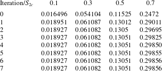
Examples of the iterative calculation of
 $S_{em}$
from initial guesses obtained from (2.39) are presented in table 1. When
 $S_{2c}\leqslant 0.3$
, it can be seen that convergence is achieved after just two iterations. When
 $S_{2c}=0.5$
, three iterations are required. When
 $S_{2c}=0.7$
, six iterations are required. The increase in the number of iterations required with increasing
 $S_{2c}$
is due to reducing validity of the
 $S_{em}\ll 1$
assumption.


2.4 Application of a similarity transform
The partial differential equation in (2.13) can be reduced to an ordinary differential equation by application of the following similarity transform
 $$\begin{eqnarray}\unicode[STIX]{x1D706}=\frac{\unicode[STIX]{x1D709}}{\unicode[STIX]{x1D70F}}.\end{eqnarray}$$
Substituting (2.40) into (2.13) and (2.22) leads to
 $$\begin{eqnarray}\frac{\text{d}F_{i}}{\text{d}C_{i}}=\unicode[STIX]{x1D706}\end{eqnarray}$$
and
 $$\begin{eqnarray}F_{i}=\unicode[STIX]{x1D6FC}_{i}-\unicode[STIX]{x1D6FD}_{i}\unicode[STIX]{x1D706}\frac{\text{d}C_{1}}{\text{d}\unicode[STIX]{x1D706}}.\end{eqnarray}$$
Differentiating both sides of (2.41) with respect to
 $C_{i}$
yields
 $$\begin{eqnarray}\frac{\text{d}^{2}F_{i}}{\text{d}C_{i}^{2}}=\frac{\text{d}\unicode[STIX]{x1D706}}{\text{d}C_{i}},\end{eqnarray}$$
which on substitution into (2.42), along with (2.41), and rearranging leads to
 $$\begin{eqnarray}\frac{\text{d}^{2}F_{1}}{\text{d}C_{1}^{2}}+\frac{\unicode[STIX]{x1D6FD}_{1}}{(F_{1}-\unicode[STIX]{x1D6FC}_{1})}\frac{\text{d}F_{1}}{\text{d}C_{1}}=0.\end{eqnarray}$$
In the event that the boundary and initial values of
 $C_{1}$
,
 $C_{10}$
and
 $C_{1I}$
, respectively, are
 $\notin (c_{12},c_{11})$
, the boundary conditions for (2.44) must satisfy the Rankine–Hugoniot conditions (similar to Orr Reference Orr2007, p. 75):
 $$\begin{eqnarray}\displaystyle & \displaystyle \frac{\text{d}F_{1}}{\text{d}C_{1}}=\frac{\unicode[STIX]{x1D6FC}_{10}-F_{1}}{C_{10}-C_{1}},\quad C_{1}\geqslant c_{11}, & \displaystyle\end{eqnarray}$$
 $$\begin{eqnarray}\displaystyle & \displaystyle \frac{\text{d}F_{1}}{\text{d}C_{1}}=\frac{\unicode[STIX]{x1D6FC}_{1I}-F_{1}}{C_{1I}-C_{1}},\quad C_{1}\leqslant c_{12}, & \displaystyle\end{eqnarray}$$
where
 $\unicode[STIX]{x1D6FC}_{10}$
and
 $\unicode[STIX]{x1D6FC}_{1I}$
represent the boundary and initial values of
 $\unicode[STIX]{x1D6FC}_{1}$
associated with
 $C_{10}$
and
 $C_{1I}$
, respectively. Alternatively, when
 $C_{10}$
and
 $C_{1I}$
are
 $\in (c_{12},c_{11})$
 $$\begin{eqnarray}\left.\begin{array}{@{}ll@{}}F_{1}=\unicode[STIX]{x1D6FC}_{10}, & C_{1}=C_{10},\\ F_{1}=\unicode[STIX]{x1D6FC}_{1I}, & C_{1}=C_{1I}.\end{array}\right\}\end{eqnarray}$$
An efficient way of expressing both (2.46) and (2.47) simultaneously is to state instead:
 $$\begin{eqnarray}\left.\begin{array}{@{}ll@{}}\displaystyle (C_{10}-C_{1})\frac{\text{d}F_{1}}{\text{d}C_{1}}+F_{1}=\unicode[STIX]{x1D6FC}_{10}, & C_{1}=\tilde{C}_{10},\\ \displaystyle (C_{1I}-C_{1})\frac{\text{d}F_{1}}{\text{d}C_{1}}+F_{1}=\unicode[STIX]{x1D6FC}_{1I}, & C_{1}=\tilde{C}_{1I},\end{array}\right\}\end{eqnarray}$$
where
 $$\begin{eqnarray}\displaystyle & \displaystyle \tilde{C}_{10}=H(C_{10}-c_{11})c_{11}+H(c_{11}-C_{10})C_{10}, & \displaystyle\end{eqnarray}$$
 $$\begin{eqnarray}\displaystyle & \displaystyle \tilde{C}_{1I}=H(c_{12}-C_{1I})c_{12}+H(C_{1I}-c_{12})C_{1I} & \displaystyle\end{eqnarray}$$
and
 $H(x)$
is a Heaviside function.
2.5 Pseudospectral solution
Following Bjornara & Mathias (Reference Bjornara and Mathias2013), the boundary value problem described in the previous section is solved using a Chebyshev polynomial differentiation matrix,
 $\unicode[STIX]{x1D63F}$
(Weideman & Reddy Reference Weideman and Reddy2000).
The coordinate space for the Chebyshev nodes is
 $x\in [-1,1]$
. However, the solution space for
 $F_{1}$
is
 $C_{1}\in [\tilde{C}_{1I},\tilde{C}_{10}]$
. Therefore the Chebyshev nodes,
 $\boldsymbol{x}$
, need to be mapped to the
 $C_{1}$
space by the following transform
 $$\begin{eqnarray}C_{1}=\frac{\tilde{C}_{10}+\tilde{C}_{1I}}{2}+\left(\frac{\tilde{C}_{10}-\tilde{C}_{1I}}{2}\right)x.\end{eqnarray}$$
Consequently, it is necessary to introduce an appropriately transformed differentiation matrix,
 $\unicode[STIX]{x1D640}$
, where
 $$\begin{eqnarray}\unicode[STIX]{x1D640}=\frac{\text{d}x}{\text{d}C_{1}}\unicode[STIX]{x1D63F}\end{eqnarray}$$
and from (2.51)
 $$\begin{eqnarray}\frac{\text{d}x}{\text{d}C_{1}}=\frac{2}{\tilde{C}_{10}-\tilde{C}_{1I}}.\end{eqnarray}$$
By applying the Chebyshev polynomial on the internal nodes and the Robin boundary conditions in (2.48) on the end nodes, equation (2.44) can be written in matrix form (similar to Piche & Kanniainen (Reference Piche and Kanniainen2009) and Bjornara & Mathias (Reference Bjornara and Mathias2013))
 $$\begin{eqnarray}\boldsymbol{R}(\boldsymbol{F})=\left[\begin{array}{@{}c@{}}\displaystyle \unicode[STIX]{x1D640}_{2:N-1,:}^{(2)}\boldsymbol{F}+\unicode[STIX]{x1D644}_{2:N-1,:}\text{diag}\left[\frac{\unicode[STIX]{x1D6FD}_{1}}{F_{1}-\unicode[STIX]{x1D6FC}_{1}}\right]\unicode[STIX]{x1D640}^{(1)}\boldsymbol{F}\\ (\boldsymbol{C}_{N}-C_{1I})\unicode[STIX]{x1D640}_{N,:}^{(1)}\boldsymbol{F}-\unicode[STIX]{x1D644}_{N,:}\boldsymbol{F}+\unicode[STIX]{x1D6FC}_{1I}\\ (\boldsymbol{C}_{1}-C_{10})\unicode[STIX]{x1D640}_{1,:}^{(1)}\boldsymbol{F}-\unicode[STIX]{x1D644}_{1,:}\boldsymbol{F}+\unicode[STIX]{x1D6FC}_{10}\end{array}\right],\end{eqnarray}$$
where
 $\boldsymbol{R}$
is the residual vector,
 $\boldsymbol{F}$
is the solution vector for the dependent variable
 $F_{1}$
,
 $\unicode[STIX]{x1D644}$
is an identity matrix,
 $\boldsymbol{C}$
is the vector containing the corresponding values of
 $C_{1}$
and
 $N$
denotes the number of Chebyshev nodes to be solved for. The two last rows on the right-hand side of (2.54) impose the Robin boundary conditions. Also note that
 $\unicode[STIX]{x1D640}^{(n)}$
can be obtained from
 $\unicode[STIX]{x1D640}^{n}$
.
The solution vector,
 $\boldsymbol{F}$
, can be obtained by Newton iteration, whereby new iterations,
 $\boldsymbol{F}_{(i+1)}$
, are obtained from
 $$\begin{eqnarray}\boldsymbol{F}_{(i+1)}=\boldsymbol{F}_{(i)}-(\unicode[STIX]{x2202}\boldsymbol{R}/\unicode[STIX]{x2202}\boldsymbol{F}_{(i)})^{-1}\boldsymbol{R}(\boldsymbol{F}_{(i)}),\end{eqnarray}$$
where
 $\unicode[STIX]{x2202}\boldsymbol{R}/\unicode[STIX]{x2202}\boldsymbol{F}$
is the Jacobian matrix defined as
 $$\begin{eqnarray}\frac{\unicode[STIX]{x2202}\boldsymbol{R}}{\unicode[STIX]{x2202}\boldsymbol{F}}=\left[\begin{array}{@{}c@{}}\displaystyle \unicode[STIX]{x1D640}_{2:N-1,:}^{(2)}+\unicode[STIX]{x1D644}_{2:N-1,:}\text{diag}\left[\frac{\unicode[STIX]{x1D6FD}_{1}}{F_{1}-\unicode[STIX]{x1D6FC}_{1}}\right]\unicode[STIX]{x1D640}^{(1)}-\unicode[STIX]{x1D644}_{2:N-1,:}\text{diag}\!\left[\text{diag}\!\left[\frac{\unicode[STIX]{x1D6FD}_{1}}{(F_{1}-\unicode[STIX]{x1D6FC}_{1})^{2}}\right]\unicode[STIX]{x1D640}^{(1)}\boldsymbol{F}\right]\\ (\boldsymbol{C}_{N}-C_{1I})\unicode[STIX]{x1D640}_{N,:}^{(1)}-\unicode[STIX]{x1D644}_{N,:}\\ (\boldsymbol{C}_{1}-C_{10})\unicode[STIX]{x1D640}_{1,:}^{(1)}-\unicode[STIX]{x1D644}_{1,:}\end{array}\right]\!.\end{eqnarray}$$
Note that
 $F_{1}$
is bounded by
 $\unicode[STIX]{x1D6FC}_{1}$
and
 $\unicode[STIX]{x1D6FC}_{10}$
. Therefore, a good initial guess is to set
 $F_{1}=\unicode[STIX]{x1D6FC}_{10}$
. Following Bjornara & Mathias (Reference Bjornara and Mathias2013), an additional correction step should be applied in the Newton iteration to force the solution,
 $F_{1}$
, to be less than
 $\unicode[STIX]{x1D6FC}_{1}$
. The Newton iteration loop is assumed to have converged when the mean absolute value of
 $\boldsymbol{R}\leqslant 10^{-9}$
. With 100 Chebyshev nodes (i.e.
 $N=100$
), convergence is typically achieved with less than 200 iterations.
2.6 Dealing with salt precipitation in the dry-out zone
Now consider the case where pure CO2 is injected into a porous medium (i.e.
 $\unicode[STIX]{x1D6FC}_{10}=1$
) initially fully saturated with brine (i.e.
 $\unicode[STIX]{x1D6FC}_{1I}=0$
). Let
 $\unicode[STIX]{x1D70E}_{32}$
be the volume fraction of NaCl in phase 2 throughout the system. In this way, the volume fraction of H2O in phase 2 prior to CO2 injection is
 $(1-\unicode[STIX]{x1D70E}_{32})$
.
Let
 $r_{0}$
[L] and
 $r_{I}$
[L] be the radial extents of the dry-out zone and injected CO2 plume respectively. At any given time, the volume of H2O evaporated by the CO2,
 $V_{e}$
[L3], can be found from
 $$\begin{eqnarray}V_{e}=2\unicode[STIX]{x03C0}\unicode[STIX]{x1D719}H(1-c_{11})\int _{r_{0}}^{r_{I}}rS_{1}\,\text{d}r.\end{eqnarray}$$
The volume of salt precipitated in the dry-out zone,
 $V_{s}$
[L3], is found from
 $$\begin{eqnarray}V_{s}=\frac{\unicode[STIX]{x1D70E}_{32}V_{e}}{1-\unicode[STIX]{x1D70E}_{32}}.\end{eqnarray}$$
The volume of the dry-out zone where the salt is precipitated,
 $V_{d}$
[L3], is found from
 $$\begin{eqnarray}V_{d}=\unicode[STIX]{x03C0}\unicode[STIX]{x1D719}Hr_{0}^{2}.\end{eqnarray}$$
Another quantity of interest is the volume of CO2 dissolved in the brine,
 $V_{c}$
[L3], which can be found from
 $$\begin{eqnarray}V_{c}=2\unicode[STIX]{x03C0}\unicode[STIX]{x1D719}Hc_{12}\int _{r_{0}}^{r_{I}}r(1-S_{1})\,\text{d}r.\end{eqnarray}$$
Considering the definition of
 $\unicode[STIX]{x1D706}$
in (2.40) in conjunction with (2.15) and (2.16)
 $$\begin{eqnarray}r_{0}^{2}=\frac{Q_{0}t\unicode[STIX]{x1D706}_{0}}{\unicode[STIX]{x03C0}\unicode[STIX]{x1D719}H}\quad \text{and}\quad r_{I}^{2}=\frac{Q_{0}t\unicode[STIX]{x1D706}_{I}}{\unicode[STIX]{x03C0}\unicode[STIX]{x1D719}H},\end{eqnarray}$$
where, recall (2.41) and (2.48),
 $\unicode[STIX]{x1D706}_{0}$
and
 $\unicode[STIX]{x1D706}_{I}$
can be found from
 $$\begin{eqnarray}\unicode[STIX]{x1D706}_{0}=\left.\frac{\text{d}F_{1}}{\text{d}C_{1}}\right|_{C_{1}=c_{11}}\quad \text{and}\quad \unicode[STIX]{x1D706}_{I}=\left.\frac{\text{d}F_{1}}{\text{d}C_{1}}\right|_{C_{1}=c_{12}}.\end{eqnarray}$$
In this way it can be understood that:
 $$\begin{eqnarray}\displaystyle & \displaystyle V_{e}=(1-c_{11})Q_{0}t\int _{\unicode[STIX]{x1D706}_{0}}^{\unicode[STIX]{x1D706}_{I}}S_{1}\,\text{d}\unicode[STIX]{x1D706}, & \displaystyle\end{eqnarray}$$
 $$\begin{eqnarray}\displaystyle & V_{d}=Q_{0}t\unicode[STIX]{x1D706}_{0}, & \displaystyle\end{eqnarray}$$
 $$\begin{eqnarray}\displaystyle & \displaystyle V_{c}=c_{12}Q_{0}t\int _{\unicode[STIX]{x1D706}_{0}}^{\unicode[STIX]{x1D706}_{I}}(1-S_{1})\,\text{d}\unicode[STIX]{x1D706}. & \displaystyle\end{eqnarray}$$
Noting that the rates at which
 $V_{s}$
and
 $V_{d}$
grow with time are constant it can also be understood that the volume fraction of precipitated salt,
 $C_{3}$
, will be both uniform within the dry-out zone and constant with time. The value of
 $C_{3}$
within the dry-out zone, hereafter denoted as
 $C_{30}$
, can be found from
 $$\begin{eqnarray}C_{30}=\frac{(1-c_{11})\unicode[STIX]{x1D70E}_{32}}{(1-\unicode[STIX]{x1D70E}_{32})\unicode[STIX]{x1D706}_{0}}\int _{\unicode[STIX]{x1D706}_{0}}^{\unicode[STIX]{x1D706}_{I}}S_{1}\,\text{d}\unicode[STIX]{x1D706}.\end{eqnarray}$$
Given that
 $C_{10}=1-C_{30}$
,
 $C_{1I}=0$
,
 $\unicode[STIX]{x1D6FC}_{10}=1$
and
 $\unicode[STIX]{x1D6FC}_{1I}=0$
, the boundary conditions in (2.48) reduce to
 $$\begin{eqnarray}\left.\begin{array}{@{}ll@{}}\displaystyle \frac{\text{d}F_{1}}{\text{d}C_{1}}=\frac{1-F_{1}}{1-C_{30}-c_{11}}, & C_{1}=c_{11},\\ \displaystyle \frac{\text{d}F_{1}}{\text{d}C_{1}}=\frac{F_{1}}{c_{12}}, & C_{1}=c_{12}.\end{array}\right\}\end{eqnarray}$$
Values of
 $C_{30}$
can be obtained iteratively by repeating the procedures outlined in § 2.5 with successive estimates of
 $C_{30}$
obtained from (2.66). Using an initial guess of
 $C_{30}=0$
, this process is found to typically converge after less than 60 iterations. The integrals in (2.65) and (2.63) can be found by trapezoidal integration.
3 Sensitivity analysis
3.1 Gas displacing oil
As a first example, the gas-displacing-oil scenario previously presented in figures 4.13 and 4.15 of Orr (Reference Orr2007) is adopted. The parameters describing the scenario include
 $c_{11}=0.95$
,
 $c_{12}=0.20$
,
 $\unicode[STIX]{x1D70E}_{32}=0$
,
 $\unicode[STIX]{x1D707}_{2}/\unicode[STIX]{x1D707}_{1}=2$
,
 $S_{1c}=0.05$
,
 $S_{2c}=0.1$
,
 $k_{r10}=k_{r20}=1$
and
 $n_{1}=n_{2}=2$
. For the pseudospectral solution, a value for the van Genuchten (Reference van Genuchten1980) parameter,
 $m$
, is set to 0.5.
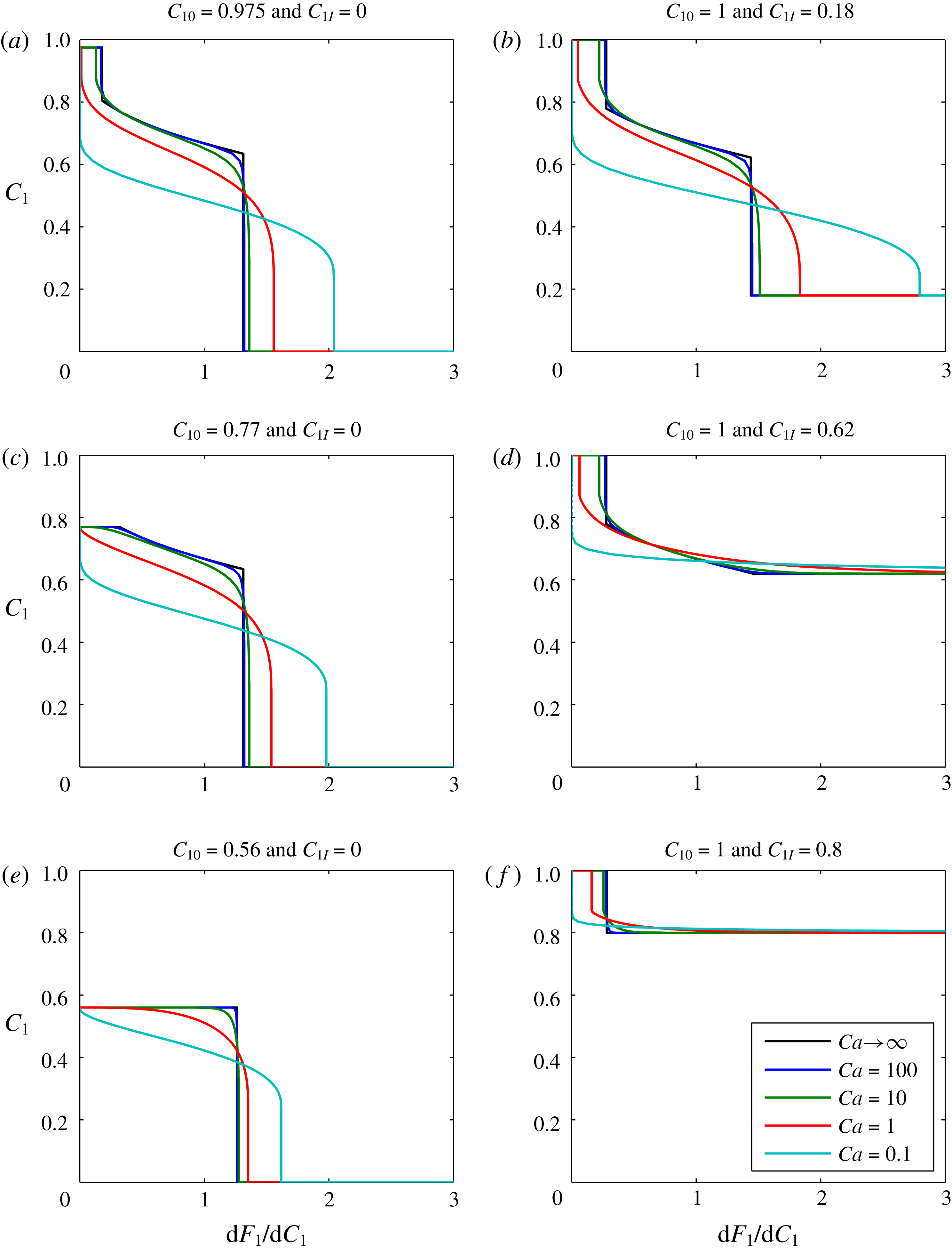
Plots of
 $C_{1}$
against
 $\text{d}F_{1}/\text{d}C_{1}$
(which, recall, is equal to
 $\unicode[STIX]{x1D709}/\unicode[STIX]{x1D70F}$
) for this scenario are shown in figure 2. The different subplots show the effect of varying the boundary volume fraction,
 $C_{10}$
, and the initial volume fraction,
 $C_{1I}$
. The different colours relate to different assumed values of
 $Ca$
. Increasing
 $Ca$
can be thought of as analogous to an increased injection rate. The
 $Ca\rightarrow \infty$
curves were obtained from the MOC solutions previously presented in figures 4.13 and 4.15 of Orr (Reference Orr2007). The finite
 $Ca$
value solutions were obtained using the pseudospectral solution described above, with 100 Chebyshev nodes.
Sensitivity analysis based on gas-displacing-oil examples. The infinite
 $Ca$
value curves were obtained from the method of characteristics solutions presented in figures 4.13 and 4.15 of Orr (Reference Orr2007). The finite
 $Ca$
value curves were obtained using the pseudospectral solution documented in the current article.
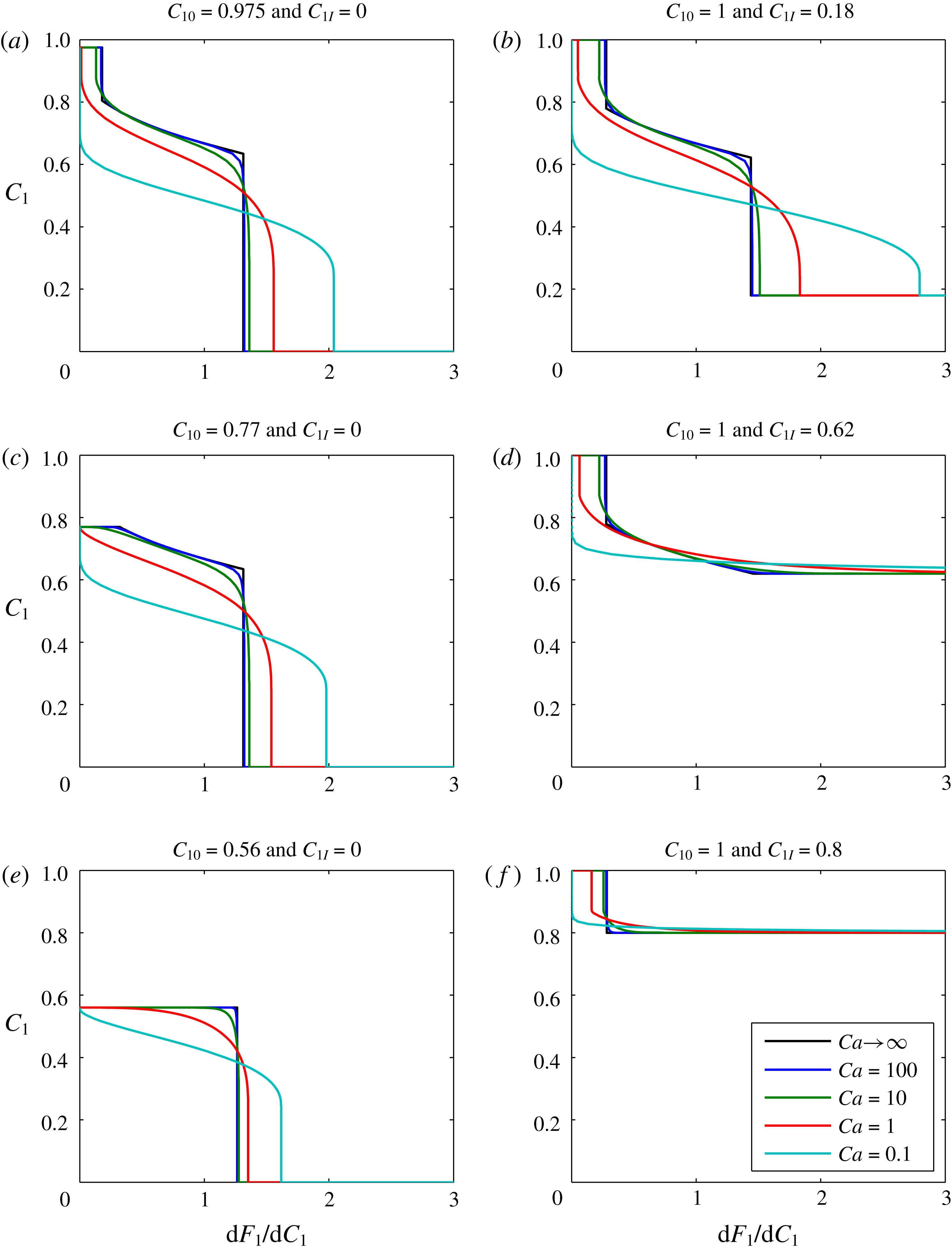
When
 $Ca=100$
, the pseudospectral solution is virtually identical to the infinite-
 $Ca$
-MOC solutions. As
 $Ca$
is decreased, the solution becomes more diffused. In figure 2(a,b,d and f), the infinity
 $Ca$
results exhibit a trailing shock, which represents a dry-out zone where all the liquid oil has been evaporated by the gas. Of particular interest is that decreasing
 $Ca$
leads to a reduction in the thickness of the dry-out zone, ultimately leading to its complete elimination.
3.2 CO2 injection in a saline formation
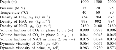
Here the CO2-injection-in-a-saline-formation scenario, previously presented by Mathias et al. (Reference Mathias, Gluyas, Gonzlez Martnez de Miguel, Bryant and Wilson2013), is revisited. The example involves injecting pure CO2 at a constant rate via a fully penetrating injection well at the centre of a cylindrical, homogenous and confined saline formation, initially fully saturated with brine. Relevant model parameters are presented in table 2. In this case, components 1, 2 and 3 are CO2, H2O and NaCl, respectively, and phases 1, 2 and 3 represent a CO2-rich phase, an H2O rich phase and precipitated salt, respectively.
Relevant model parameters used for the CO2 injection in saline formation scenario, previously presented by Mathias et al. (Reference Mathias, Gluyas, Gonzlez Martnez de Miguel, Bryant and Wilson2013).
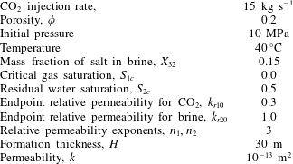
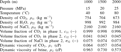
The relevant fluid properties are obtained using equations of state (EOS) and empirical equations provided by Batzle & Wang (Reference Batzle and Wang1992), Fenghour, Wakeham & Vesovic (Reference Fenghour, Wakeham and Vesovic1998), Spycher et al. (Reference Spycher, Pruess and Ennis-King2003) and Spycher & Pruess (Reference Spycher and Pruess2005). Mathias et al. (Reference Mathias, Gonzalez Martinez de Miguel, Thatcher and Zimmerman2011a ) found that when using analytical solutions in this context, to account for the relatively high compressibility of CO2, it is important to use an estimate of the final pressure rather than the initial pressure for calculating the fluid properties relating to CO2. Mathias et al. (Reference Mathias, Gluyas, Gonzlez Martnez de Miguel, Bryant and Wilson2013) found that, for the scenario described in table 2, the well pressure increased by just over 5 MPa after 10 years. Therefore, for the current study, fluid properties are calculated using 15 MPa as opposed to 10 MPa.
The EOS of Spycher et al. (Reference Spycher, Pruess and Ennis-King2003) and Spycher & Pruess (Reference Spycher and Pruess2005) provide equilibrium mole fractions as opposed to volume fractions. Pruess & Spycher (Reference Pruess and Spycher2007) show how mole fractions can be converted to mass fractions,
 $x_{ij}$
[-], which can be converted to volume fractions,
 $\unicode[STIX]{x1D70E}_{ij}$
[-], using (similar to Orr Reference Orr2007, p. 19)
 $$\begin{eqnarray}\unicode[STIX]{x1D70E}_{ij}=\frac{\unicode[STIX]{x1D70C}_{j}x_{ij}}{\unicode[STIX]{x1D70C}_{ij}},\end{eqnarray}$$
where
 $\unicode[STIX]{x1D70C}_{ij}$
[ML-3] is the density of component
 $i$
in phase
 $j$
and
 $\unicode[STIX]{x1D70C}_{j}$
[ML-3] is the composite phase density, which can be found from
 $$\begin{eqnarray}\unicode[STIX]{x1D70C}_{j}=\left(\mathop{\sum }_{i=1}^{N_{c}}\frac{x_{ij}}{\unicode[STIX]{x1D70C}_{ij}}\right)^{-1},\end{eqnarray}$$
where
 $N_{c}$
[-] is the number of components present. Because the pseudospectral solution above assumes component densities remain constant throughout, a decision is made that
 $\unicode[STIX]{x1D70C}_{12}=\unicode[STIX]{x1D70C}_{11}$
,
 $\unicode[STIX]{x1D70C}_{21}=\unicode[STIX]{x1D70C}_{22}$
and
 $\unicode[STIX]{x1D70C}_{32}=\unicode[STIX]{x1D70C}_{33}$
.
Table 3 shows how the various fluid properties vary with depth below sea level in this context. Depth is related to pressure by assuming hydrostatic conditions and then adding 5 MPa to allow for pressure induced by CO2 injection. Depth is related to temperature by assuming a geothermal gradient of
 $40\,^{\circ }\text{C}~\text{km}^{-1}$
. It can be seen that the volume fractions are largely unaffected by depth. However, the variation in brine viscosity and CO2 density are more noticeable.
Relevant model parameters used for the CO2 injection in a saline formation scenario with a brine salinity of 150 ppt.
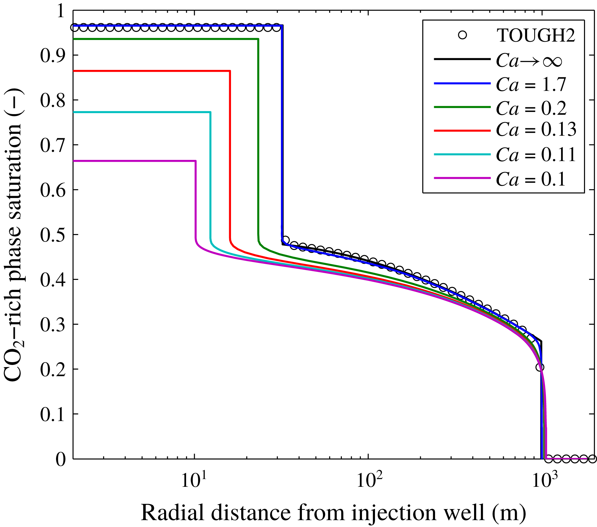
A comparison of results from the pseudospectral solution with those from the TOUGH2 simulation reported by Mathias et al. (Reference Mathias, Gluyas, Gonzlez Martnez de Miguel, Bryant and Wilson2013) is shown in figure 3, alongside results for when
 $Ca\rightarrow \infty$
, obtained using a MOC solution similar to that previously presented by Zeidouni et al. (Reference Zeidouni, Pooladi-Darvish and Keith2009) and Mathias et al. (Reference Mathias, Gluyas, Gonzlez Martnez de Miguel and Hosseini2011b
). Mathias et al. (Reference Mathias, Gluyas, Gonzlez Martnez de Miguel, Bryant and Wilson2013) assumed
 $P_{c0}=19.6$
kPa. Considering the other parameters in tables 2 and 3, this leads to a
 $Ca$
value of 1.7. There is excellent correspondence between the MOC solution, the TOUGH2 results and the pseudospectral solution when
 $Ca=1.7$
.
Plots of CO2 saturation against radial distance after injecting 4.73 Mt of CO2 whilst assuming a range of different capillary numbers,
 $Ca$
. The TOUGH2 results are from the simulations previously presented by Mathias et al. (Reference Mathias, Gluyas, Gonzlez Martnez de Miguel, Bryant and Wilson2013). Other associated model parameters are presented in table 2. The results for
 $Ca\rightarrow \infty$
were obtained using a method of characteristics solution, also presented by Mathias et al. (Reference Mathias, Gluyas, Gonzlez Martnez de Miguel, Bryant and Wilson2013). The results for finite
 $Ca$
values were obtained using the pseudospectral solution.

A value of
 $P_{c0}=19.6$
kPa is often used to describe saline formations in a CO2 storage context (Rutqvist et al.
Reference Rutqvist, Birkholzer, Cappa and Tsang2007; Zhou et al.
Reference Zhou, Birkholzer, Tsang and Rutqvist2008; Mathias et al.
Reference Mathias, Gluyas, Gonzlez Martnez de Miguel, Bryant and Wilson2013; Zhu et al.
Reference Zhu, Zuo, Zhang, Zhang, Wang and Wang2015, e.g.). Experimental analysis looking at four different sandstone reservoirs revealed a range of
 $P_{c0}$
values from 1.3–7.1 kPa (Oostrom et al.
Reference Oostrom, White, Porse, Krevor and Mathias2016). Smaller values of
 $P_{c0}$
imply larger pore diameters.
A hallmark of hyperbolic theory is that the problem can be reduced to a fundamental wave structure which constitutes the solution. In figure 3, it can be seen that such a wave structure is largely preserved, despite the inclusion of capillary diffusion. Furthermore, the wave velocity of the leading shock is virtually independent of
 $Ca$
for the range of
 $Ca$
values studied. However, decreasing
 $Ca$
leads to a more diffused spreading wave caused by the increase in capillary diffusion, which in turn leads to a reduction in the wave velocity of the trailing shock, as also seen in figure 2(a). The decrease in steady-state CO2 saturation in the dry-out zone is caused by an increase in the volume fraction of precipitated salt (recall that
 $C_{10}=1-C_{30}$
).
For the scenarios depicted in figure 3,
 $C_{30}$
is found to be insensitive to
 $Ca$
for
 $Ca$
values greater than or equal to 1.7. However for
 $Ca$
values less than 1.7, the volume of the dry-out zone is significantly reduced and the volume fraction of precipitated salt is significantly increased. The value of
 $C_{30}$
for
 $Ca=0.2$
is almost double the value for
 $Ca=1.7$
. The value of
 $C_{30}$
for
 $Ca=0.1$
is around 10 times that of when
 $Ca=1.7$
. The
 $Ca=1.7$
scenario described in table 2 assumes an injection rate of
 $15~\text{kg}~\text{s}^{-1}$
. The results shown in figure 3 therefore suggest that reducing the injection rate down to
 $1.8~\text{kg}~\text{s}^{-1}$
would lead to a doubling of the volume fraction of precipitated salt around the injection well. Furthermore, reducing the injection rate from
 $15~\text{kg}~\text{s}^{-1}$
down to
 $0.9~\text{kg}~\text{s}^{-1}$
would lead to an almost 10 times larger volume fraction of precipitated salt around the injection well.
Plots of
 $F_{1}$
,
 $\unicode[STIX]{x1D6FC}_{1}$
and
 $\unicode[STIX]{x1D6FD}_{1}$
against
 $C_{1}$
for the simulation results presented in figure 3.

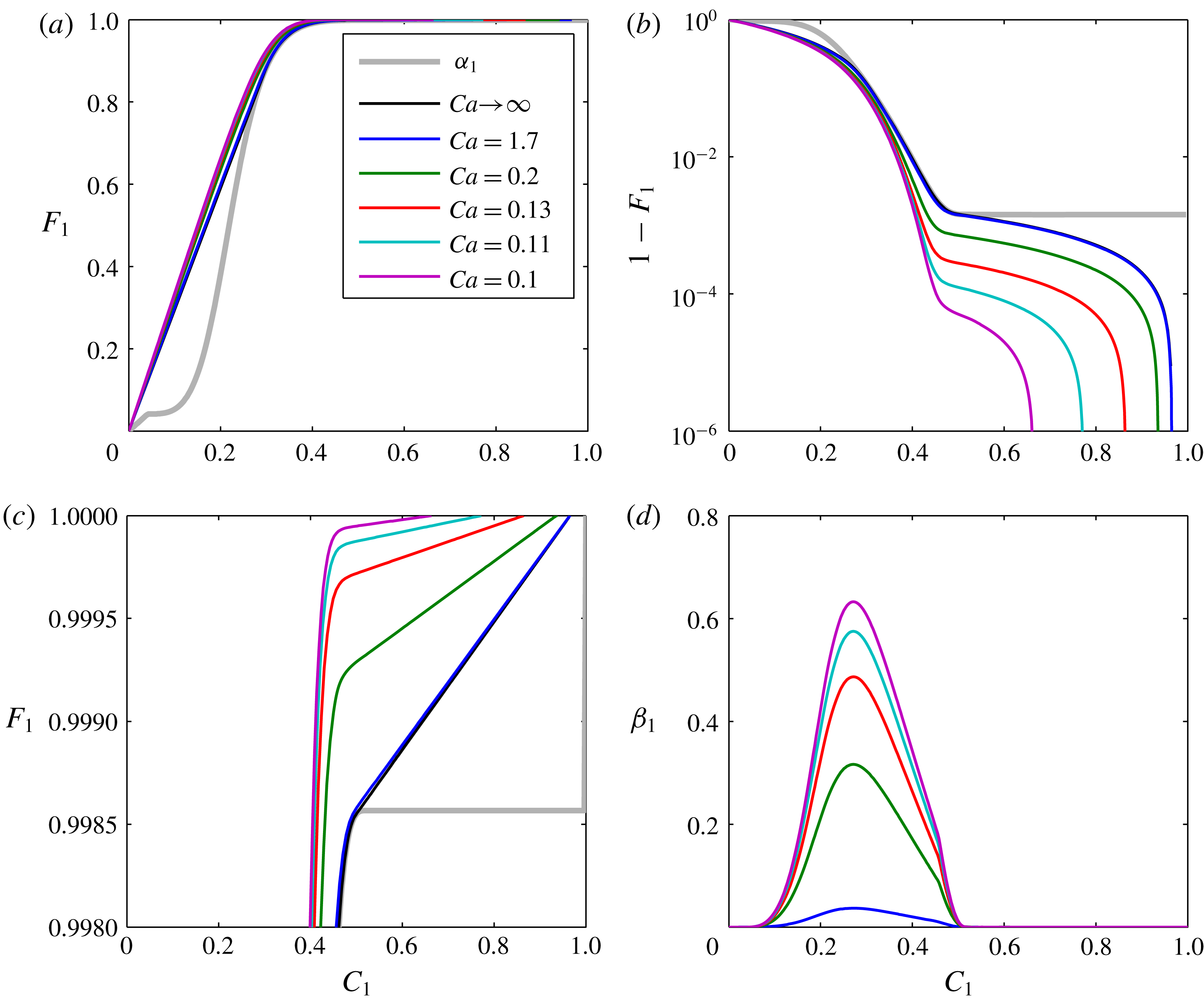
For the hyperbolic case when
 $Ca\rightarrow \infty$
, it is common to study plots of
 $F_{1}$
and
 $C_{1}$
(Orr Reference Orr2007). Figure 4(a) shows plots of
 $F_{1}$
against
 $C_{1}$
for all the values of
 $Ca$
presented in figure 3 along with a plot of
 $\unicode[STIX]{x1D6FC}_{1}$
. The MOC solution (i.e. with
 $Ca\rightarrow \infty$
), which sits almost exactly underneath the
 $Ca=1.7$
line, intersects the
 $\unicode[STIX]{x1D6FC}_{1}$
line at tangents, which is symptomatic of satisfying the shock waves satisfying the Rankine–Hugoniot condition. To better visualize the results for finite
 $Ca$
values,
 $(1-F_{1})$
is shown on a log scale in figure 4(b). Here it can be seen that the models approach a value of
 $F_{1}=1$
at different
 $C_{1}$
values depending on the volume fraction of precipitated salt. The volume fraction of precipitated salt increases with decreasing
 $Ca$
. Figure 4(c) shows a close-up view of the trailing shocks on linear axes for further reference. For finite
 $Ca$
values, the
 $F_{1}$
lines never actually intersect the
 $\unicode[STIX]{x1D6FC}_{1}$
line except at where
 $C_{1}=0$
. The reason for this is due to
 $\unicode[STIX]{x1D6FD}_{1}$
, which is plotted in figure 4(d). The highest values of
 $\unicode[STIX]{x1D6FD}_{1}$
are at the centre of the two-phase region,
 $C_{1}\in (c_{12},c_{11})$
.
 $\unicode[STIX]{x1D6FD}_{1}$
smoothly grades down to zero as it reaches the single-phase regions,
 $C_{1}\notin (c_{12},c_{11})$
.
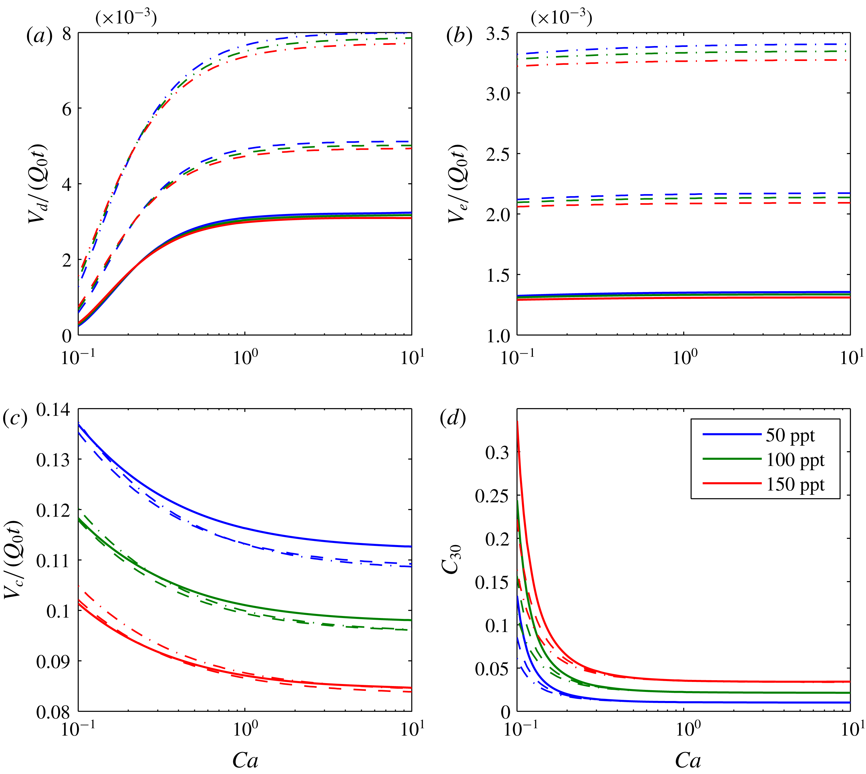
A further sensitivity analysis is presented in figure 5. The three depth scenarios presented in table 3 are applied with three different brine salinities. Figure 5(a) shows how the volume of the dry-out zone decreases with decreasing
 $Ca$
. The size of the dry-out zone increases with increasing depth. In contrast, brine salinity has very little impact on dry-out zone volume.
Sensitivity analysis based around the scenario presented in figure 3. The different colours relate to different brine salinities, as indicated in the legend. The solid lines, dashed lines and dash-dotted lines represent results obtained using fluid properties calculated assuming the saline formation exists at a depth of 1000 m, 1500 m and 2000 m, respectively (based on hydrostatic pressure conditions and a geothermal gradient of
 $40\,^{\circ }\text{C}~\text{km}^{-1}$
as in table 3). (a) Shows plots of the ratio of dry-out zone volume (
 $V_{d}$
) to injected CO2 volume (
 $Q_{0}t$
) against capillary number (
 $Ca$
). (b) Shows plots of the ratio of volume of evaporated water (
 $V_{e}$
) to
 $Q_{0}t$
against
 $Ca$
. (c) Shows plots of the ratio of volume of dissolved CO2 (
 $V_{c}$
) to
 $Q_{0}t$
against
 $Ca$
. (d) Shows plots of precipitated salt volume fraction in the dry-out zone (
 $C_{30}$
) against
 $Ca$
.

Figure 5(b) shows the volume of the evaporated water also reduces with decreasing
 $Ca$
. At first this seems surprising given that capillary pressure effects should bring more water into the dry-out zone. However, the effect of the capillary pressure is also to spread the CO2 out further (see leading edge of CO2 plumes in figure 3). As a consequence, more CO2 is dissolved (see figure 5
c). Consequently, less of the CO2-rich phase is available for water from the brine to evaporate into. The volume of evaporated water increases with depth because the equilibrium volume fraction of water in the CO2-rich phase increases with depth (see table 3). The volume of dissolved CO2 is insensitive to depth but decreases with increasing brine salinity. The latter is because the solubility limit of CO2 in brine decreases substantially with increasing salinity (Spycher & Pruess Reference Spycher and Pruess2005).
Figure 5(d) shows how volume fraction of precipitated salt in the dry-out zone,
 $C_{30}$
, superlinearly increases with decreasing
 $Ca$
. For
 $Ca>0.25$
, the quantity of precipitated salt is mostly controlled by brine salinity. However, for
 $Ca<0.25$
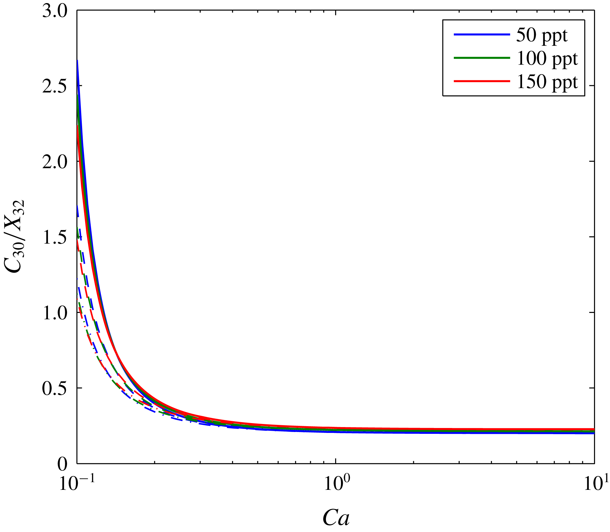
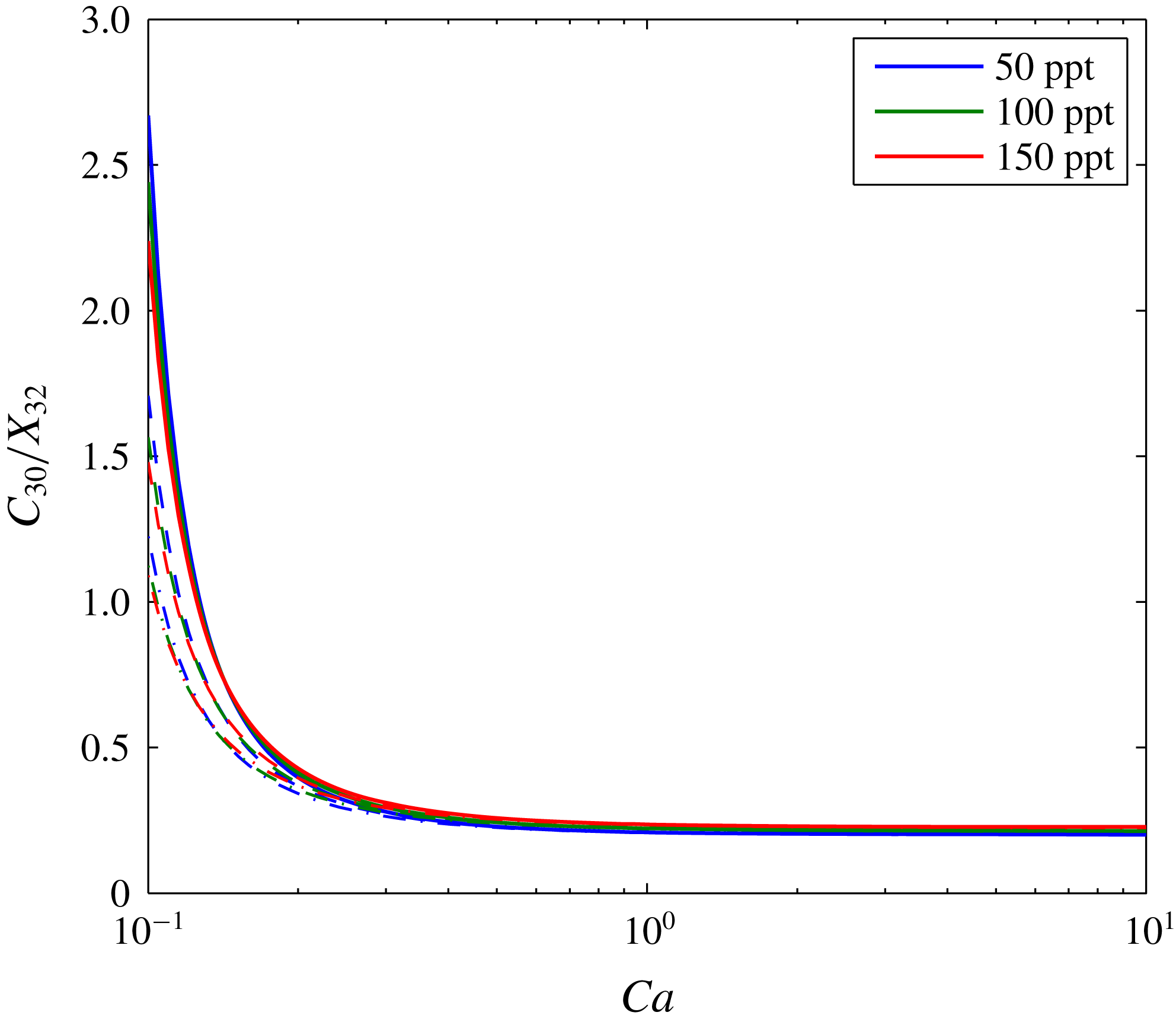
, depth plays an increasingly important role, with higher levels of salt precipitation in shallower formations. This is because the dry-out zone increases with depth, despite increasing water evaporation with depth. Figure 6 shows the same results as figure 5(d) but with
 $C_{30}$
normalized by dividing by the salinity of the brine,
 $X_{32}$
. Here it can be seen that
 $C_{30}$
almost linearly scales with
 $X_{32}$
.
The same as figure 5(d) except that salt volume fraction,
 $C_{30}$
, is divided by the salinity of the brine,
 $X_{32}$
.
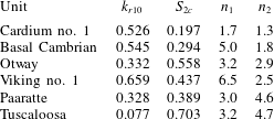
The volume fraction of precipitated salt is also strongly controlled by the relative permeability parameters,
 $k_{rj0}$
,
 $S_{jc}$
and
 $n_{j}$
(Zhang et al.
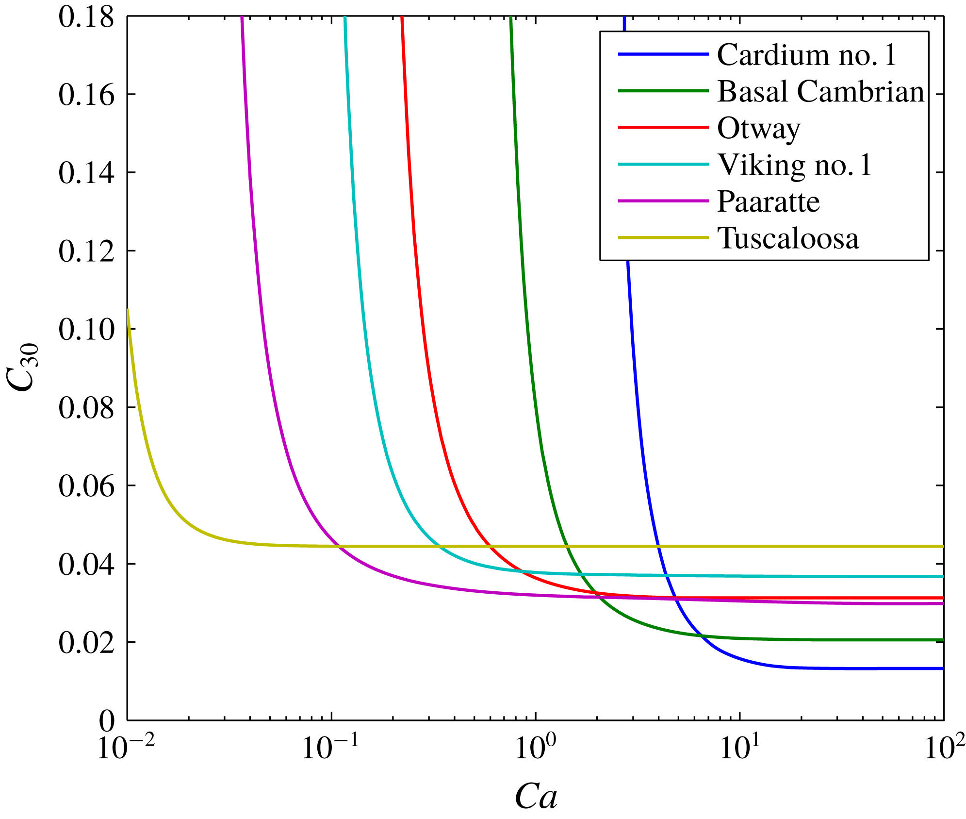
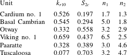
Reference Zhang, Oostrom and White2016). The analysis performed to provide figure 6 was repeated for the 1000 m depth scenario for each of the six groups of relative permeability parameters presented in table 4. These six parameter sets were selected from a database of 25 core experiments previously compiled by Mathias et al. (Reference Mathias, Gluyas, Gonzlez Martnez de Miguel, Bryant and Wilson2013). The six cores were selected to provide a representative range of possible outcomes, given the wide variability generally observed in such data sets.
From figure 7 it can be seen that the high
 $Ca$
values of
 $C_{30}$
range from 0.019 to 0.044. Furthermore, the critical
 $Ca$
value below which
 $C_{30}$
superlinearly increases ranges from 0.025 to 10. Comparing these results with the parameter sets in table 4 it can be seen that when the relative permeability for brine is more linear, the value of
 $C_{30}$
at high values of
 $Ca$
tends to be lower. However, this linearity also leads to the superlinearly increasing of
 $C_{30}$
with decreasing
 $Ca$
to occur at a relatively low value of
 $C_{30}$
(see for example Cardium no. 1 and Basal Cambrian). Exactly the opposite happens when the relative permeability for brine is highly nonlinear (see for example Paaratte and Tuscaloosa). This is probably due to counter-current flow of water being less efficient when relative permeability is highly nonlinear.


Relative permeability parameters for six different sandstone cores (after Mathias et al.
Reference Mathias, Gluyas, Gonzlez Martnez de Miguel, Bryant and Wilson2013). Note that for each core
 $k_{r20}=1$
and
 $S_{1c}=0$
. Data for Cardium no. 1, Basal Cambrian and Viking no. 1 were originally obtained by Bennion & Bachu (Reference Bennion and Bachu2008). Data for Otway were originally obtained by Perrin & Benson (Reference Perrin and Benson2010). Data for Paaratte and Tuscaloosa were originally obtained by Krevor et al. (Reference Krevor, Pini, Zuo and Benson2012).
4 Discussion of key modelling assumptions
4.1 Incompressible fluids
Fluid densities are assumed to be independent of pressure. The compressibilities of H2O and NaCl are commonly ignored. For pressures and temperatures associated with depleted gas reservoirs, the compressibility of CO2 is very high and has a significant impact on fluid movement (Mathias et al. Reference Mathias, McElwaine and Gluyas2014). However, for CO2 injection in saline formations, fluid pressures are expected to be hydrostatic or above. Under these conditions, providing a sensible reference pressure is used to determine the fluid properties of CO2 (i.e. an estimate of pressure towards the end of the injection cycle), the compressibility of CO2 has been found to have a negligible effect in this context (Mathias et al. Reference Mathias, Gonzalez Martinez de Miguel, Thatcher and Zimmerman2011a ,Reference Mathias, Gluyas, Gonzlez Martnez de Miguel and Hosseini b ).
4.2 No volume change on mixing
Component densities are assumed to be uniform across phases. In fact, the densities of CO2 and H2O are both higher in the aqueous phase as compared to in the CO2-rich phase. For a wide range of different CO2 injection scenarios, this volume change on mixing is found to lead to an increase in volumetric flow rate of around 0.05 % in Zone 2 and a decrease in volumetric flow rate of around 5 % in Zone 3 (see table 2 of Mathias et al. Reference Mathias, Gluyas, Gonzlez Martnez de Miguel and Hosseini2011b ). See § 2.1 above for an explanation of the zone numbers.
With regards to NaCl, the density of precipitated NaCl,
 $\unicode[STIX]{x1D70C}_{33}$
, is
 $2160~\text{kg}~\text{m}^{-3}$
. Using (3.2) in conjunction with the EOS for brine given by Batzle & Wang (Reference Batzle and Wang1992), it can be shown that the density of NaCl dissolved in brine,
 $\unicode[STIX]{x1D70C}_{32}$
, is around
 $2800~\text{kg}~\text{m}^{-3}$
. In the above analysis we have set
 $\unicode[STIX]{x1D70C}_{32}=\unicode[STIX]{x1D70C}_{33}$
such that the model precipitates the correct volume of salt in the dry-out zone. The consequence is that the volume fractions of water and CO2 in the brine are underestimated by around 2 %.
Figure 3 compares model results from TOUGH2 with those from the similarity solution. TOUGH2 properly incorporates fluid compressibility and volume change on mixing and there is negligible difference between the two models.
4.3 Ignoring gravity effects
As stated earlier, another important assumption is that the vertical permeability of the formation is sufficiently low that gravity effects can be ignored. Extreme changes in density and/or viscosity can lead to instabilities and fingering phenomena, which cannot be represented using one-dimensional models. Indeed, Kim et al. (Reference Kim, Han, Oh, Kim and Kim2012) found that buoyancy driven flow, associated with the different densities of brine and CO2, played an important part in controlling the spatial distribution of precipitated salt around an injection well. However, this was mostly after the cessation of injection. During the injection phase, gravity segregation within the dry-out zone was much less significant and no viscous fingering was observed.
Mathias et al. (Reference Mathias, Gluyas, Gonzlez Martnez de Miguel and Hosseini2011b ) presented a comparison of simulation results where gravity was accounted for and ignored using TOUGH2 and the MOC solution of Zeidouni et al. (Reference Zeidouni, Pooladi-Darvish and Keith2009), respectively. For a 100 m thick isotropic saline formation, gravity was found to have a strong effect on the leading edge of the CO2 plume. However, gravity effects were found to be negligible on the dry-out zone development and the associated volume fraction of the precipitated salt. For a 50 m thick isotropic saline formation, gravity effects were found to be negligible throughout.
The dry-out zone is generally unaffected by gravity segregation due to the larger velocities situated close around the injection well, which are mostly horizontal due to the horizontal driving force provided by the injection well boundary (Mathias et al. Reference Mathias, Gluyas, Gonzlez Martnez de Miguel and Hosseini2011b ). From the discussion above it is expected that gravity effects are unlikely to significantly affect the dry-out zone in the 30 m thick saline formations studied in this current article, at least for the lower capillary numbers studied. However, as the capillary numbers are increased, the horizontal injection velocities will become less significant and gravity will play a more important role. However, our analysis has shown that excessive salt precipitation can also develop in the absence of gravity effects due to the counter-current imbibition associated with capillary pressure.
5 Summary and conclusions
A new similarity solution has been presented to study the role of capillary pressure on salt precipitation during CO2 injection in a saline formation. Dimensional analysis has revealed that the problem is largely controlled by a capillary number,
 $Ca=Q_{0}\unicode[STIX]{x1D707}_{1}/(4\unicode[STIX]{x03C0}HkP_{c0})$
, where
 $H$
[L] is the formation thickness,
 $k$
[L2] is permeability,
 $P_{c0}$
[ML-1T-2] is an air-entry pressure associated with the porous medium,
 $Q_{0}$
[L3T-1] is the injection rate and
 $\unicode[STIX]{x1D707}_{1}$
[ML-1T-1] is the dynamic viscosity of CO2. The volume fraction of precipitated salt around the injection well,
 $C_{30}$
[-], is found to superlinearly increase with decreasing
 $Ca$
. Subsequent sensitivity analysis also reveals that
 $C_{30}$
linearly scales with the salinity of brine.
 $C_{30}$
is found to reduce with increasing storage depth. This latter point is largely attributed to the equilibrium volume fraction of water in the CO2-rich phase increasing with depth. Relative permeability parameters are found to have a significant effect on the value of
 $Ca$
below which
 $C_{30}$
superlinearly increases. For highly nonlinear relative permeabilities,
 $C_{30}$
remains stable for much lower capillary numbers.
The new similarity solution represents a significant extension of the work of Zeidouni et al. (Reference Zeidouni, Pooladi-Darvish and Keith2009) by accounting for capillary pressure and an extension of the work of Bjornara & Mathias (Reference Bjornara and Mathias2013) by accounting for radially symmetric flow, partial miscibility and salt precipitation.
In one scenario studied, reducing the CO2 injection rate from
 $15~\text{kg}~\text{s}^{-1}$
to
 $0.9~\text{kg}~\text{s}^{-1}$
led to almost a 10 times larger volume fraction of precipitated salt. In the past, pressure buildup in injection wells has been widely perceived to increase monotonically with CO2 injection rate. However, these results clearly demonstrate that as injection rate is decreased the volume fraction of precipitated salt around the injection well will significantly increase leading to potentially significant loss of injectivity. It follows that below a critical threshold, pressure buildup can be expected to increase with reducing injection rates as well. The similarity solution presented in this article can serve as a useful tool to determine the critical capillary number at which these effects are likely to take place.
Acknowledgement
This work was funded by the Crown Estate.