1. Introduction
Thermoacoustic systems containing premixed flames have been shown to exhibit periodic, period-2, quasiperiodic and chaotic behaviour in both experiments (Gotoda & Ueda Reference Gotoda and Ueda2002; Gotoda et al. Reference Gotoda, Asano, Chuah and Kushida2009; Kabiraj et al. Reference Kabiraj, Saurabh, Wahi and Sujith2012a ; Kabiraj, Sujith & Wahi Reference Kabiraj, Sujith and Wahi2012b ) and numerical simulations (Kashinath, Hemchandra & Juniper Reference Kashinath, Hemchandra and Juniper2012; Kashinath & Juniper Reference Kashinath and Juniper2012; Kashinath, Waugh & Juniper Reference Kashinath, Waugh and Juniper2013b ). The type of nonlinear behaviour observed in the long time limit (the attractor) is often very sensitive to the parameters of the system and the oscillation’s initial amplitude and form. For example, there can be a sudden change in the system’s behaviour (i) when a parameter is varied, which indicates a bifurcation of the system in parameter space, or (ii) when the initial amplitude passes some threshold, which indicates mode switching within a multistable region of parameter space (Kashinath et al. Reference Kashinath, Waugh and Juniper2013b ).
In the frequency domain, Noiray et al. (Reference Noiray, Durox, Schuller and Candel2008) used the flame describing function (FDF) approach (Dowling Reference Dowling1999) to estimate the location of Hopf bifurcations and fold bifurcations and to explain the mode switching that they had observed experimentally. The FDF approach assumes that the acoustic velocity and pressure signals are harmonic. This is a severe limitation in thermoacoustic systems because it precludes all nonlinear behaviour apart from fixed points and period-1 oscillations. The next-simplest forms of nonlinear behaviour, period-doubling and quasiperiodicity, which start at period-doubling and Neimark–Sacker bifurcations, respectively, would require knowledge of the flame’s response to a forcing signal composed of two harmonic oscillations. The FDF would then need to be a function of four variables (the frequency and amplitude of each harmonic signal) and would be extremely expensive to obtain. Experiments in this direction show that it is possible to obtain the flame’s response to forcing at two commensurate frequencies (Balachandran, Dowling & Mastorakos Reference Balachandran, Dowling and Mastorakos2008) and two non-commensurate frequencies (Moeck & Paschereit Reference Moeck and Paschereit2012). However, these studies convincingly show that this response is not the sum of the responses at each individual frequency, demonstrating that there is no short cut, i.e. the FDF would need to be found as a function of all four variables. More complex nonlinear behaviour, such as multiperiodic (frequency locked) and chaotic behaviour, would require the FDF as a function of multiple frequencies and amplitudes and would therefore be impossibly expensive to obtain. Nevertheless, all of the types of nonlinear behaviour described above are frequently observed in experiments and simulations, highlighting the need for an alternative to the FDF approach.
In the time domain, there are two broad approaches: (i) energy balance techniques, and (ii) autonomous dynamical system techniques. Energy balance techniques examine the growth of acoustic energy around a cycle. Heckl has recently used Green’s functions to transfer an approximation of experimental FDF data into the time domain, in the form of an amplitude-dependent time delay and gain (Heckl Reference Heckl2013a
,Reference Heckl
b
). Whilst this approach can be used to examine the energy balance of a single frequency at a set amplitude, it cannot be used to examine the temporal evolution of the system. This is because amplitude-dependent coefficients cannot be used with a Green’s function framework because the evolution relies on linear superposition. Furthermore, because both Heckl’s method and the CIRCE method of Kashinath et al. (Reference Kashinath, Hemchandra and Juniper2012) assume a harmonic form for the acoustic perturbations, they suffer from the same limitations described in the previous paragraph for frequency domain methods. Alternative methods have been used to transfer FDF data into the time domain, by using impulse responses derived theoretically from the
 $G$
-equation (Blumenthal et al.
Reference Blumenthal, Subramanian, Sujith and Polifke2013) or from system identification of CFD data (Selimefendigil, Sujith & Polifke Reference Selimefendigil, Sujith and Polifke2011). Whilst these impulse responses can provide insight into competing flame processes, such as convection and restoration, they can only be used for linear analysis.
Autonomous dynamical system techniques describe the system using a state vector that evolves in time according to a set of nonlinear equations. These techniques do not make any a priori assumptions about the form of the acoustic velocity and pressure signals that arise from the model and can therefore display all types of nonlinear behaviour. For example, Kashinath et al. (Reference Kashinath, Waugh and Juniper2013b
) used time-domain simulations to find the regions of parameter space at which a model of a ducted premixed flame exhibited period-1, period-
 $2^{n}$
, multiperiodic, quasiperiodic and chaotic behaviour. They also examined the corresponding attractors in phase space and revealed the role that unstable attractors play in mode switching.
Time domain simulations have several limitations, however, when they are used to identify attractors in phase space. First, they are computationally expensive because typically they must calculate several hundred cycles in order for the system to converge to an attractor to some tolerance. Second, they can converge only to stable attractors, although they sometimes remain sufficiently close to an unstable attractor for this attractor to be estimated. Third, it is difficult to show which aspects of the thermoacoustic system are responsible for the qualitative changes in nonlinear behaviour observed at bifurcations, because it often requires prohibitive numbers of long timemarches to converge to a bifurcation with sufficient accuracy. It should be noted that if the bifurcation can be found to sufficient accuracy, however, then the Floquet multipliers and modes can be estimated by timemarching from an unstable limit cycle that is very close to the bifurcation, taking a snapshot of the state vector every period of the limit cycle for several periods, then applying dynamic mode decomposition to the snapshots (Schmid Reference Schmid2010). Some iteration or interpolation will be required to ensure the snapshots are taken at exact multiples of the limit cycle period, or the accuracy of the Floquet multipliers will be limited by the size of the time step.
These three limitations can be overcome by combining time domain simulations with continuation analysis. This allows fixed points, limit cycles and bifurcations to be tracked as the system parameters are varied. Continuation analysis converges much faster to limit cycles (period-1, period-2, etc.) than time domain simulations alone. It can also converge to stable and unstable limit cycles and, by calculating the Floquet multipliers of these limit cycles, can reveal the type of bifurcation that occurs when a limit cycle changes from stable to unstable. The eigenvectors corresponding to (i) eigenvalues around fixed points or (ii) Floquet multipliers around limit cycles reveal the coupled flame–acoustic motion that causes the change in behaviour. These eigenvectors can then be used to identify the optimal passive control mechanisms to delay or even prevent these bifurcations from occurring (Magri & Juniper Reference Magri and Juniper2013) and hold great promise for the passive control of thermoacoustic systems.
In a previous paper, we showed that matrix-free continuation methods can efficiently find limit cycles of a relatively large thermoacoustic system (Waugh, Illingworth & Juniper Reference Waugh, Illingworth and Juniper2013). The model used in that paper, which was of a ducted diffusion flame, was only weakly nonlinear and therefore did not display period-
 $2^{n}$
or quasiperiodic behaviour. In this paper, we demonstrate matrix-free continuation methods on a model of a ducted axisymmetric premixed flame using a kinematic
 $G$
-equation solver. This flame model has strongly nonlinear behaviour because it can form cusps and pinched-off pockets. We find period-1 and period-2 limit cycles, as well as fold, period-doubling and Neimark–Sacker bifurcations. We find these as functions of two system parameters: the location of the flame in the duct and the aspect ratio of the steady flame. The matrix-free continuation methods and the underlying numerical techniques are described fully in Waugh et al. (Reference Waugh, Illingworth and Juniper2013). Their application to the ducted premixed flame model is described fully in Waugh (Reference Waugh2013).
This paper has three aims: (i) to demonstrate that continuation algorithms can efficiently find the limit cycles and bifurcations of a thermoacoustic system containing a premixed flame model; (ii) to identify the types of bifurcation by examining the Floquet multipliers of the limit cycles; (iii) to identify the coupled flame–acoustic motion that is responsible for the qualitative change in behaviour at each bifurcation by analysing the eigenvectors associated with the unstable Floquet multipliers. Whilst the results compare qualitatively well with experimental data, no quantitative comparisons are made, because the model used is too simplistic, particularly in its treatment of the acoustics. These limitations are due to the model, however, and not the analysis techniques that are the focus of this paper.
The paper is organised as follows. Section 2 describes the thermoacoustic model, which is of a ducted premixed flame. Section 3 describes the continuation methods used to find the limit cycles. These sections summarise previous papers and further details can be found in Waugh (Reference Waugh2013) and Waugh et al. (Reference Waugh, Illingworth and Juniper2013). Section 4 then describes the specific numerics required to adapt the coupled
 $G$
-equation model for use with the continuation methods. Section 5 then presents the limit cycles of the ducted premixed flame model, their subsequent bifurcations and the causes of those bifurcations. The paper then concludes.
2. Model description
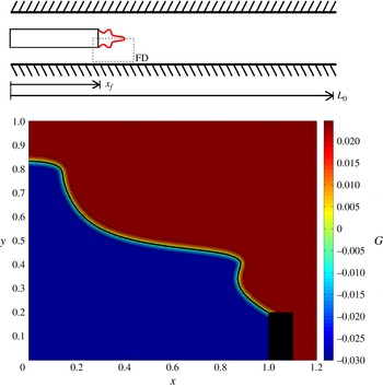
The ducted premixed flame model used in this paper consists of a one-dimensional acoustic duct coupled to an axisymmetric flame domain, as shown in figure 1. In the acoustic domain, the velocity,
 $u$
, and pressure,
 $p$
, are discretised using a Galerkin modal expansion:
 $$\begin{eqnarray}u(x,t)=\mathop{\sum }\limits_{j=1}^{N}{\it\eta}_{j}(t)\cos (\,j{\rm\pi}x),\quad p(x,t)=-\mathop{\sum }\limits_{j=1}^{N}\left(\frac{{\it\eta}_{j}(t)}{j{\rm\pi}}\right)\sin (\,j{\rm\pi}x).\end{eqnarray}$$
Using the non-dimensionalisations
 $u={\tilde{u}}/{\tilde{u}}_{0}$
,
 $p=\tilde{p}/{\it\gamma}M\tilde{p}_{0}$
,
 $x=\tilde{x}/\tilde{L}_{0}$
,
 $t=\tilde{t}\tilde{c}_{0}/\tilde{L}_{0}$
, the non-dimensional momentum and energy equations for the acoustic velocity and pressure are
 $$\begin{eqnarray}\displaystyle & \displaystyle \frac{\partial u}{\partial t}+\frac{\partial p}{\partial x}=0 & \displaystyle\end{eqnarray}$$
 $$\begin{eqnarray}\displaystyle & \displaystyle \frac{\partial p}{\partial t}+\frac{\partial u}{\partial \tilde{x}}+{\it\zeta}p-{\it\beta}_{T}\dot{Q}{\it\delta}\left(x-x_{f}\right)=0 & \displaystyle\end{eqnarray}$$
 $$\begin{eqnarray}{\it\beta}_{T}=\frac{\left({\it\gamma}-1\right)\tilde{\dot{Q}}_{0}{\it\alpha}}{{\it\gamma}\tilde{p}_{0}{\tilde{u}}_{0}}\quad \text{and}\quad \dot{Q}=\frac{\tilde{\dot{Q}}}{\tilde{\dot{Q}}_{0}}\end{eqnarray}$$
where
 ${\it\zeta}$
is a modal damping coefficient, which when discretised is
 ${\it\zeta}_{j}=c_{1}j^{2}+c_{2}\sqrt{j}$
, where
 $j$
is the mode number of the Galerkin expansion, and
 $c_{1}$
and
 $c_{2}$
are constants. Additional definitions are the ratio between the burner width and duct width,
 ${\it\alpha}$
, the heat release,
 $\dot{Q}$
, the Dirac delta function,
 ${\it\delta}(x)$
, the ratio of specific heats,
 ${\it\gamma}$
, and a subscript of 0 for a mean quantity. This model of the acoustic duct is the same as that used by Balasubramanian & Sujith (Reference Balasubramanian and Sujith2008) and Juniper (Reference Juniper2011).
Schematic of the one-dimensional acoustic duct (a) and the axisymmetric flame domain (b). The flame domain contains a
 $G$
-field that is a signed distance function from the flame surface (wavy black line) in a thin band around the flame. The flame domain is labelled as FD in the acoustic duct, and is rotated 90° anticlockwise in the bottom frame.

In the flame domain, the premixed flame propagates in a direction that is normal to the local flame surface. We use the
 $G$
-equation method, in which the flame surface is defined as the zero contour of a scalar field and the flame normals are defined by the local gradient of the scalar field (Dowling Reference Dowling1999; Schuller, Durox & Candel Reference Schuller, Durox and Candel2003; Hemchandra, Preetham & Lieuwen Reference Hemchandra, Preetham and Lieuwen2007). This kinematic
 $G$
-equation is solved on an imposed velocity field, using a level set method. This allows pinch-off and multivalued (highly wrinkled) flame shapes. We also use a rotating boundary condition at the base of the flame (Waugh Reference Waugh2013), which allows movement of the flame anchoring point and flashback, both of which generate these wrinkles. The evolution in time of the
 $G$
-field is given by
 $$\begin{eqnarray}\frac{\partial G}{\partial t}+\boldsymbol{U}\boldsymbol{\cdot }\boldsymbol{{\rm\nabla}}\boldsymbol{G}-s_{L}\left|\boldsymbol{{\rm\nabla}}\boldsymbol{G}\right|=0\end{eqnarray}$$
where
 $s_{L}$
is the flame speed and
 $\boldsymbol{U}$
is the velocity vector in the flame field. The flame speed in this paper depends on the local curvature and, for a conical flame of aspect ratio
 ${\it\beta}$
, is given by
 $$\begin{eqnarray}s_{L}=\frac{u_{0}}{\sqrt{1+{\it\beta}^{2}}}\left(1+M_{{\it\kappa}}{\it\kappa}_{axi}\right)\end{eqnarray}$$
where
 $M_{{\it\kappa}}$
is a non-dimensionalised Markstein length and
 ${\it\kappa}_{axi}$
is the signed axisymmetric curvature (Hemchandra, Shreekrishna & Lieuwen Reference Hemchandra, Shreekrishna and Lieuwen2010). Curvature is a second-order quantity, which means that a significant drop in timestep is required in order to ensure that the CFL condition is met. Strain effects are not included in the flame speed because this is not appropriate with the current velocity model (the velocity model has uniform velocity gradient in the
 $y$
direction).
When the equivalence ratio is uniform and the domain is axisymmetric, the heat release rate is
 $$\begin{eqnarray}\dot{Q}_{axi}={\it\rho}s_{L0}\left({\it\phi}\right)h_{R}\left({\it\phi}\right)\int _{D}2{\rm\pi}r\left(1+M_{{\it\kappa}}{\it\kappa}_{axi}\right)\left|\boldsymbol{{\rm\nabla}}\boldsymbol{G}\right|{\it\delta}(G)\,\text{d}r\,\text{d}z.\end{eqnarray}$$
The
 $G$
-equation is simulated using a modified version of the LSGEN2D code developed by Hemchandra (Reference Hemchandra2009), who used it to analyse the response of premixed flames to acoustic forcing (Hemchandra et al.
Reference Hemchandra, Preetham and Lieuwen2007) and to equivalence ratio fluctuations (Hemchandra et al.
Reference Hemchandra, Shreekrishna and Lieuwen2010). The code uses a local level-set method, a fifth-order weighted essentially non-oscillatory (WENO) procedure to take derivatives (Jiang & Peng Reference Jiang and Peng2000), and, in this study, the HCR-2 method of Hartmann, Meinke & Schröder (Reference Hartmann, Meinke and Schröder2010) to reinitialise the
 $G$
-field.
A simple velocity model is applied to the flame domain. Experiments on premixed flames have shown that acoustic perturbations cause waves to advect down the flame (Birbaud, Durox & Candel Reference Birbaud, Durox and Candel2006). These waves typically advect more slowly than the mean flow. In this paper, acoustic perturbations start at the burner lip and are propagated downstream with the one-dimensional advection equation (Hemchandra et al.
Reference Hemchandra, Preetham and Lieuwen2007; Preetham Reference Preetham2007; Kashinath et al.
Reference Kashinath, Hemchandra and Juniper2012). The velocity field is therefore the time history of the acoustic perturbation at the burner lip, i.e. the further a point is from the burner lip, the earlier the acoustic disturbance at that point was generated. These perturbations travel at a speed of
 $u_{0}/K$
, where
 $K$
is between 1.0 and 1.5 (Kashinath, Hemchandra & Juniper Reference Kashinath, Hemchandra and Juniper2013a
). In numerical studies, the value of
 $K$
has been shown to have a strong influence on the nonlinear behaviour of premixed flames (Kashinath et al.
Reference Kashinath, Hemchandra and Juniper2012). In particular, subcritical Hopf bifurcations are more prevalent at high values of
 $K$
, and this leads to more parameter regions that are bistable. The transverse velocity is calculated from the continuity equation applied to the unburnt mixture within the flame.
In summary, this velocity model uses a relatively simple formulation but produces similar flame shapes to those seen in experiments at lower amplitudes, such as those of Birbaud et al. (Reference Birbaud, Durox and Candel2006) which reach amplitudes of
 $u_{f}=0.2$
. Experimental flame images are not available for direct comparison at the higher fluctuation amplitudes shown by the results, but previous studies suggest that the
 $G$
-equation can produce comparable results at higher amplitudes. In particular, Dowling (Reference Dowling1999) found self-excited oscillations beyond
 $u_{f}=1.0$
and her results compared satisfactorily with those of Bloxsidge, Dowling & Langhorne (Reference Bloxsidge, Dowling and Langhorne1988), and Shin, Plaks & Lieuwen (Reference Shin, Plaks and Lieuwen2011) compared experimental bluff body results satisfactorily against
 $G$
-equation simulations for similar amplitudes as this paper. The combination of the simple velocity model with a
 $G$
-equation method causes some non-physical behaviour, however, such as that the mean heat release rate decreases as the forcing amplitude increases, which is a common feature of this type of method (Oberlack & Cheviakov Reference Oberlack and Cheviakov2010). The acoustic model contains some simplifications: there is no temperature jump in the duct, the flame is acoustically compact and the acoustic damping model is based on simple coefficients at particular frequencies. With these simplifications, the model shows the same qualitative behaviour as comparable experiments (Kabiraj et al.
Reference Kabiraj, Sujith and Wahi2012b
), but we do not suggest that it is suitable for quantitative comparisons.
3. Matrix-free continuation methods for finding limit cycles
A brief summary of the matrix-free continuation methods used to find limit cycles is given in this section. Complete details are given in Waugh (Reference Waugh2013).
Continuation methods examine nonlinear systems whose evolution is governed by
 $$\begin{eqnarray}\frac{\text{d}\boldsymbol{x}(t)}{\text{d}t}=F(\boldsymbol{x}(t),{\it\lambda}),\quad \boldsymbol{x}(t)\in \mathbb{R}^{N}\end{eqnarray}$$
where
 $\boldsymbol{x}$
is the current state of the system,
 ${\it\lambda}$
are parameters and
 $N$
is the number of variables in the state vector. The governing equations are in most cases derived from the discretisation of a PDE.
Limit cycles satisfy
 $$\begin{eqnarray}\boldsymbol{x}(0)=\boldsymbol{x}(T),\quad \left\{T\in \mathbb{R}^{+}|T\neq 0\right\},\end{eqnarray}$$
where
 $T$
is the period of the cycle. Further constraints are required if the model contains an explicit time delay, which are described in Waugh (Reference Waugh2013). Note that the model described in § 2 implicitly contains a time delay (between velocity perturbations and subsequent heat release), however, because the velocity field includes convection.
A shooting method is used in this paper to iterate towards a limit cycle. The shooting method finds, by iteration, a state on the limit cycle and the period of the limit cycle. The current guess for a state on the limit cycle,
 $\boldsymbol{x}(0)$
, is iterated in order to satisfy the condition for a limit cycle, which is that
 $\boldsymbol{x}(0)=\boldsymbol{x}(T)$
, where
 $\boldsymbol{x}(T)$
is found with a timemarching process. Numerically, the iteration process is stopped when a specific level of convergence is reached,
 $\left\Vert \boldsymbol{x}(T)-\boldsymbol{x}(0)\right\Vert <{\it\epsilon},\ \left\{{\it\epsilon}\in \mathbb{R}^{+}|{\it\epsilon}\neq 0\right\}$
, where
 ${\it\epsilon}$
is small.
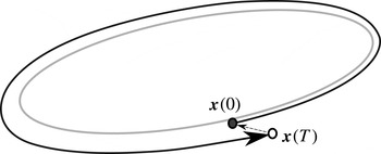
The magnitude of the residual vector,
 $\boldsymbol{r}=\boldsymbol{x}(0)-\boldsymbol{x}(T)$
(figure 2), is reduced to a predefined tolerance by a two-step iteration process. First, we consider the evolution of the system when started from small perturbations around the current guess
 $[\boldsymbol{x}(0),T]$
. We generate a
 $(N+1)\times (N+1)$
Jacobian matrix, which relates a general small change in
 $[\boldsymbol{x}(0),T]$
to the resulting change in
 $[\boldsymbol{x}(0)-\boldsymbol{x}(T),{\it\theta}]$
, where
 ${\it\theta}$
is a phase condition described later. Second, we solve a linear equation with the Jacobian matrix to find the
 $[{\rm\Delta}\boldsymbol{x},{\rm\Delta}T]$
that we should add to our current guess,
 $[\boldsymbol{x}(0),T]$
, in order to move closer to the limit cycle. If the magnitude of the residual is still too large, we repeat the first step from the improved guess.
Standard shooting method to find a limit cycle (grey loop). Given a current guess for a state on a limit cycle,
 $\boldsymbol{x}(0)$
, we timemarch forward
 $T$
time units to
 $\boldsymbol{x}(T)$
, where
 $T$
is our guess for the period. We then iterate our starting guess,
 $\boldsymbol{x}(0)$
, to minimise the length of the residual vector,
 $\boldsymbol{x}(0)-\boldsymbol{x}(T)$
(dashed arrow).

Equation (3.3) shows the linear equation for the
 $n$
th iteration, where
 $i$
and
 $j$
are the row and column indices of the matrix (Roose et al.
Reference Roose, Lust, Champneys and Spence1995). It has the standard form for multidimensional Newton iteration,
 $\boldsymbol{\mathsf{J}}{\rm\Delta}\boldsymbol{x}=-\boldsymbol{r}$
:

 $$\begin{eqnarray}\mathop{M_{i,j}}\limits^{N\times N}=\frac{\partial \boldsymbol{x}_{i}(T)}{\partial \boldsymbol{x}_{j}(0)},\quad \mathop{\boldsymbol{b}_{i}}\limits^{N\times 1}=-\frac{\partial \boldsymbol{x}_{i}(T)}{\partial T},\quad \mathop{\boldsymbol{c}_{j}}\limits^{1\times N}=\frac{\partial {\it\theta}}{\partial \boldsymbol{x}_{j}(0)},\quad \mathop{d}\limits^{1\times 1}=\frac{\partial {\it\theta}}{\partial T}\end{eqnarray}$$
 $$\begin{eqnarray}\boldsymbol{x}(0)^{n+1}=\boldsymbol{x}(0)^{n}+{\rm\Delta}\boldsymbol{x},\quad T^{n+1}=T^{n}+{\rm\Delta}T.\end{eqnarray}$$
There is an infinite number of points on a limit cycle that satisfy
 $\boldsymbol{r}=0$
, however, so a condition is required to fix the phase of the limit cycle
 $\left({\it\theta}\right)$
and therefore provide a unique solution state. In this paper, the phase condition is, arbitrarily, that the instantaneous amplitude in the first acoustic mode is zero,
 ${\it\eta}_{1}=0$
.
In (3.3), the characteristics of the system are contained in the monodromy matrix
 $\boldsymbol{\mathsf{M}}$
, which relates a change in
 $\boldsymbol{x}(0)$
to a change in
 $\boldsymbol{x}(T)$
. The eigenvalues of the monodromy matrix are called Floquet multipliers. In a dissipative system, such as in thermoacoustics, most of the Floquet multipliers are clustered near zero. These correspond to quickly dissipated motions, because a change in
 $\boldsymbol{x}(0)$
causes very little change in
 $\boldsymbol{x}(T)$
. The remaining few Floquet multipliers are not clustered near zero. These correspond to the bulk motions of the system, because a change in
 $\boldsymbol{x}(0)$
causes a significant change in
 $\boldsymbol{x}(T)$
. These bulk motions govern the flame–acoustic interaction.
The
 $j$
th column of the Jacobian matrix can be numerically found in two ways: either by perturbing
 $\boldsymbol{x}_{j}(0)$
and then timemarching forward and measuring the resultant change in
 $\boldsymbol{x}(T)$
, or by timemarching the first variational equations (tangent linear equations). The latter approach is used in the Navier–Stokes continuation of Sanchez (Sánchez et al.
Reference Sánchez, Net, García-Archilla and Simó2004; Sánchez & Net Reference Sánchez and Net2010). To fill the Jacobian matrix for each linear equation,
 $N$
timemarches are therefore required. For large thermoacoustic systems, with
 $O(10^{3})$
variables, it is impractical to form the Jacobian matrices because the computational expense of timemarching is too high.
Matrix-free methods are those that solve the linear equation,
 $\boldsymbol{\mathsf{J}}{\rm\Delta}\boldsymbol{x}=-\boldsymbol{r}$
, without ever requiring the matrix
 $\boldsymbol{\mathsf{J}}$
to be explicitly defined. These methods are iterative and only require calculation of matrix–vector products, i.e.
 $\boldsymbol{\mathsf{J}}\mathbf{v}$
, where
 $\mathbf{v}$
is an arbitrary vector. This differs from many conventional methods of solving linear equations, where the matrix
 $\boldsymbol{\mathsf{J}}$
is defined and then decomposed. In this paper, the matrix-free generalised minimal residual method (GMRES) (Saad & Schultz Reference Saad and Schultz1986) is used to solve the linear equations. GMRES has been used recently by several authors for matrix-free continuation and it shows promise as a method of analysing complex fluid systems (Salinger et al.
Reference Salinger, Lehoucq, Pawlowski and Shadid2002; Sánchez, Marques & Lopez Reference Sánchez, Marques and Lopez2002; Sánchez et al.
Reference Sánchez, Net, García-Archilla and Simó2004; Viswanath Reference Viswanath2007; Sánchez & Net Reference Sánchez and Net2010; Erdogan et al.
Reference Erdogan, Thies, Wubs and Dijkstra2011; Chandler & Kerswell Reference Chandler and Kerswell2013).
Matrix-free methods require accurate evaluations of general matrix–vector products (
 $\boldsymbol{\mathsf{J}}\mathbf{v}$
). In the case of the Jacobian matrix, the matrix–vector product can be approximated by finite differences because the Jacobian matrix is formed of partial derivatives (Georg Reference Georg2001). In this section, a mapping operator,
 $A$
, which represents the time marching process, is defined as
 $\boldsymbol{x}(T)=A\left(\boldsymbol{x}(0)\right)$
. The spatial part of the Jacobian matrix is defined in (3.3), and can be written as
 $$\begin{eqnarray}\mathsf{J}_{ij}=\frac{\partial \left(\boldsymbol{x}_{i}(0)-\boldsymbol{x}_{i}(T)\right)}{\partial \boldsymbol{x}_{j}(0)}.\end{eqnarray}$$
The matrix–vector product for an arbitrary vector
 $\mathbf{v}$
can therefore be approximated by (3.7), where
 ${\it\delta}$
is small:
 $$\begin{eqnarray}\boldsymbol{\mathsf{J}}\mathbf{v}=\mathbf{v}-\frac{A(\boldsymbol{x}(0)+{\it\delta}\mathbf{v})-A(\boldsymbol{x}(0))}{{\it\delta}}+O({\it\delta}).\end{eqnarray}$$
4. Adaptation for matrix-free continuation methods
To perform continuation methods, a suitable state vector must be defined. The state vector is a snapshot of the system at an instant in time. For continuation methods, the state vector must obey three principles. First, the state vector must contain all of the information required to describe the system at that instant in time. It should be possible to restart the simulation exactly from the state vector alone; time traces of any variable or derived quantity should show no sign of a restart having occurred. Second, the state vector should contain no information that is not required to describe the state of the system: each variable in the state vector must contain some independent information. Otherwise, if a dependent quantity is included in the state vector, then the state vector may become inconsistent when perturbed by the continuation algorithm. Third, the state vector must have a suitable form for perturbation. This last principle is subtle and often problem specific.
To make the state vector suitable for perturbation, it is important to weight the variables such that a fixed size perturbation to any variable affects the system’s behaviour to a similar degree. This means that the Jacobian matrix will be better conditioned, and therefore easier to solve with iterative methods, and also means that a 2-norm of the state vector is appropriate to indicate convergence. For example, a perturbation of size
 $10^{-2}$
on a pressure value of
 $10^{5}$
Pa would have almost no effect on the system’s behaviour, but the same perturbation on a mixture fraction value might have a significant effect on system behaviour: in this case the pressure value should be scaled down. Note that the rationale behind the scaling is not to simply non-dimensionalise perturbations by a mean quantity, although this often has a similar effect.
Further consideration is required if finite difference matrix–vector products are used. Finite difference matrix–vector products for limit cycles were defined in (3.7) to be
 $\boldsymbol{\mathsf{J}}\mathbf{v}=\mathbf{v}-(A(\boldsymbol{x}(0)+{\it\delta}\mathbf{v})-A(\boldsymbol{x}(0)))/{\it\delta}+O({\it\delta})$
. The accuracy of the matrix–vector product is therefore dependent on both the size of the perturbation,
 ${\it\delta}$
, and the level of noise in the timemarching process. The value of
 ${\it\delta}$
should be small for an accurate matrix–vector product (to be approximately linear), but must also be large enough that the effect of the perturbation is not lost in the timemarching noise. A noisy timemarching process therefore means that a larger value of
 ${\it\delta}$
must be used, which in the case of the premixed flame model, limits which discretisations can be used to define the flame shape. This is discussed further in the next subsection.
4.1. Discretisation of the flame shape
In the premixed flame model of this paper, the state vector must include the state of the acoustic field, the state of the velocity field and the state of the
 $G$
-field. In the previous section, it was established that variables that do not contain any independent information should not be included in the state vector, because it leads to inconsistencies when the state vector is perturbed. The
 $G$
-field is a good example of this. The
 $G$
-field is described entirely by the location of the flame surface because the signed distance function is a one-to-one mapping: each flame shape defines a unique
 $G$
-field, and each
 $G$
-field defines a unique flame shape.
It would be inappropriate to include the entire
 $G$
-field in the state vector because when the state vector is perturbed the
 $G$
-field will no longer be a signed distance function. This is because each value of
 $G$
in the two-dimensional field is not independent, it is defined by the location of the flame surface, and therefore it cannot be varied independently.
The only information in the
 $G$
-field is the shape of the flame surface. The state vector must therefore include a discretised version of this flame shape. The flame shape is a two-dimensional curve, which may have multiple cusps, and may have multiple separate sections (during pinch-off). The discretisation used to describe the flame shape must satisfy four conditions. First, the discretisation must define a unique two-dimensional shape to a suitable level of accuracy. Second, the size of the discretisation must not change when the flame surface is perturbed slightly, because the state vector must not change size during the solution of each linear equation (3.3). Third, the discretisation must be suitable for comparing two flame shapes; as much as is possible, the discretisation should allow easy comparison between the same parts of a curve. This is not the case with arclength based discretisations (see later in this section). Fourth, the flame shape must remain smooth when a small but finite perturbation is added to the discretisation to take a matrix–vector product; during evaluation of the matrix–vector product, the perturbation of size
 ${\it\delta}$
should not cause the flame shape to form loops or subgrid size ripples.
Several approaches have been considered for discretising the flame shape, which can be divided roughly into arclength-based approaches and fixed location-based approaches. A few of these approaches are discussed in this subsection and evaluated against the four criteria in the previous paragraph. The discretisations are generally inappropriate during pinch-off or flashback, but that does not mean that the continuation methods cannot find limit cycles that contain pinch-off/flashback. Pinch-off and flashback generally occur for only a fraction of the limit cycle, so a limit cycle can be found if the phase of the cycle is fixed such that there is no pinch-off or flashback in the starting state,
 $\boldsymbol{x}(0)$
. This is because the continuation methods see the timemarching process as a black box that maps an input state,
 $\boldsymbol{x}(0)$
, to an output state,
 $\boldsymbol{x}(T)$
, and therefore if the pinch-off phenomena is within a single timemarch then it cannot affect the continuation methods.
Arclength-based approaches discretise the flame shape by storing quantities as a function of cumulative arclength,
 $s$
. Because the length of the flame will change but the size of the discretisation must remain constant, it is better to store quantities in terms of normalised arclength,
 ${\hat{s}}=s/s_{TOTAL}$
, and to store the total arclength,
 $s_{TOTAL}$
, separately. One arclength approach would be to define two functions,
 $x=f_{1}({\hat{s}})$
and
 $y=f_{2}({\hat{s}})$
. Another arclength approach would be to define the curvature of the flame shape,
 ${\it\kappa}=f({\hat{s}})$
, and the angle of the flame shape at the burner lip,
 ${\it\phi}_{0}$
. By integrating the curvature function twice, it is possible to recreate the two-dimensional flame shape (Miller Reference Miller2009). Arclength-based approaches have the significant advantage that functions of arclength are always single valued. Arclength-based approaches have two main disadvantages, however: first, the process of calculating arclength (and curvature) generates errors which affect matrix–vector product accuracy; and second, it is not easy to compare the same parts of a curve when using normalised arclength. This latter disadvantage is important with iterative methods. For example, imagine comparing two flame shapes that are identical near the burner but different near the centreline. Even where the flames are identical, the values of the discretisation are different, because the length of the two flames is different and therefore the discretisation points have moved along the flame surface. This makes it harder for the iterative algorithms to reduce the residual between two flame shapes, because they cannot operate solely on a small section of the flame; to reduce the difference between flame shapes over a small section of the flame requires all of the values in the discretisation to be changed.
The simplest fixed location approach would be to evaluate the curve as a function
 $y=f(x)$
, by storing
 $y$
values of the flame surface at fixed
 $x$
locations. This is simple but does not allow the function
 $f$
to be multivalued, and therefore cannot discretise cusps. This discretisation has been used before in flame-tracking models for linear stability analysis of premixed flames (Ducruix, Durox & Candel Reference Ducruix, Durox and Candel2000; Schuller et al.
Reference Schuller, Durox and Candel2003), where amplitudes are small and sharp cusps do not occur.
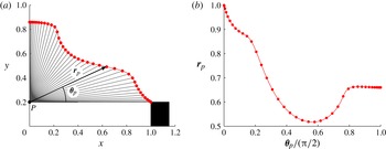
A fixed location approach based on polar coordinates is chosen to generate the results in this paper. The discretisation is shown schematically in figure 3. A reference point (P) is placed at the centreline at the level of the burner lip. The flame shape is then defined in polar coordinates from this point, with Chebyshev spacing in
 ${\bf\theta}_{p}$
between 0 and
 ${\rm\pi}/2$
, to form a function
 $\boldsymbol{r}_{p}=f({\bf\theta}_{p})$
. The subscript
 $p$
is used to denote that this is the radius from the reference point, not the radius from the burner centreline. The Chebyshev discretisation ensures high accuracy and a smooth function over
 ${\bf\theta}_{p}$
. The discretisation is not perfect: it will fail if cusps are sharp and near the centreline, because
 $\boldsymbol{r}_{p}$
will no longer be a single-valued function of
 ${\bf\theta}_{p}$
. The discretisation also clusters points near the start and end of the curve, which may lead to subgrid size ripples when a large number of points is used.
Discretisation method based on polar coordinates. A reference point,
 $p$
, is placed at the centre point level with the burner lip. The flame shape is described by the radius from the reference point,
 $\boldsymbol{r}_{p}=f({\bf\theta}_{p})$
, with a Chebyshev spacing in
 ${\bf\theta}_{p}$
.

It should be noted that the shape of the bifurcation diagrams found by the continuation methods is set by the model and its discretisation, not the
 ${\bf\theta}_{p}$
discretisation. The mesh and form of the
 ${\bf\theta}_{p}$
discretisation control whether it is possible for the continuation methods to converge. If the size of the
 ${\bf\theta}_{p}$
discretisation is too large then the smallest gap between points is much smaller than a cell, which artificially introduces numerical ripples onto the fitted flame surface. This results in divergence or extremely poor convergence. If the size of the
 ${\bf\theta}_{p}$
discretisation is too small then the largest gap between points is many cells across, which cannot capture the flame shape accurately. This generally results in divergence or poor convergence, but it is possible that the continuation could converge to a false solution where the flame shape at
 $\boldsymbol{x}(0)$
and
 $\boldsymbol{x}(T)$
match at the points stored in
 ${\bf\theta}_{p}$
, but is wildly different in between them. Because the flame shapes in this paper are relatively smooth, however, this situation is only possible when the
 ${\bf\theta}_{p}$
discretisation seriously under-resolves the flame shape. Nevertheless, several limit cycles were examined to check that the convergence was valid. At the convergence level of
 $\Vert \boldsymbol{x}(0)-\boldsymbol{x}(T)\Vert <5\times 10^{-4}$
that is used in the results section, the flame shapes were nowhere more than a tenth of a grid cell different between the start and end of a limit cycle.
For the parameter regions studied in this paper and the choice of phase condition, this discretisation was able to capture the flame shapes without failing.
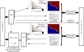
Figure 4 shows a summary of the discretisation process, and shows how the GMRES solver of the continuation methods interacts with the LSGEN2D
 $G$
-equation solver. The LSGEN2D timemarching routine is written in C, but the continuation routines and interface routines are written in MATLAB. The continuation routines and interface routines require negligible computational time compared with the timemarching routine.
Schematic of the interface between the GMRES solver and the LSGEN2D
 $G$
-equation code. The GMRES solver gives a new state vector,
 $\boldsymbol{x}(0)$
, which contains values for: the polar coordinate discretisation of the flame shape, the acoustic Galerkin modes,
 $\left[\boldsymbol{{\it\eta}}(0);\dot{\boldsymbol{{\it\eta}}}(0)\right]$
, the vertical velocity field,
 $\mathbf{v}(0)$
, the current guess for the period,
 $T$
, and a continuation parameter,
 ${\it\lambda}$
, if arclength continuation is used. To form the input file for LSGEN2D, the
 $G$
-contours must be created from the flame shape, and fixed parameters must be added. The LSGEN2D code then timemarches for
 $T$
time units. The zero contour of the
 $G$
-field at time
 $T$
must then be discretised to form the state vector
 $\boldsymbol{x}(T)$
. The residual vector is then created and fed back into GMRES.

5. Results
The first aim of this paper is to demonstrate that these matrix-free continuation methods can efficiently find the limit cycles and bifurcations of this thermoacoustic system. To do this, we have created a bifurcation diagram in which two parameters are varied: the flame location in the duct,
 $x_{f}$
, and the aspect ratio of the flame,
 ${\it\beta}=\sqrt{(u_{0}/s_{L})^{2}-1}$
. The constant parameters are
 ${\it\phi}=1.0$
,
 ${\it\alpha}=0.7$
,
 $K=1.5$
,
 $M_{{\it\kappa}}=0.04$
,
 $L_{0}=1$
,
 ${\it\rho}_{0}=1.16\ \text{kg}\ \text{m}^{-3}$
,
 $p_{0}=10^{5}\ \text{Pa}$
,
 ${\it\gamma}=1.4$
,
 $c_{1}=0.012$
and
 $c_{2}=0.024$
.
The
 $G$
-field is discretised on a
 $401\times 401$
grid with spacing 0.005 and local level set regions 12 grid cells wide. A timestep of
 $1.5\times 10^{-4}$
is used with 14 reinitialisation steps per timestep, with reinitialisation Courant number of 0.5. The Chebyshev polar coordinate discretisation of the flame surface has 150 points. A total of 20 Galerkin modes are used for the acoustics.
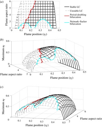
Bifurcation surface of period-1 limit cycles as two parameters are varied: the flame location in the duct,
 $x_{f}$
, and the flame aspect ratio,
 ${\it\beta}$
. The bifurcation surface is composed of over 600 limit cycles, each converged to
 $\Vert \boldsymbol{x}(0)-\boldsymbol{x}(T)\Vert <5\times 10^{-4}$
. In the three-dimensional plots, the vertical axis is the maximum acoustic velocity at the flame. The surface has regions with unstable limit cycles (dashed grey lines) and regions with stable limit cycles (solid black lines), whose boundaries are defined by the locations of the period-doubling bifurcation (red line) and the Neimark–Sacker bifurcation (cyan line). In (a) we show the surface from above and in (b) and (c) we show the same three-dimensional surface from two different views.

5.1. Bifurcation surfaces
Figure 5 shows the bifurcation surface of period-1 limit cycles, whose frequencies are close to that of the fundamental acoustic mode, measured in terms of the peak
 $u_{f}$
during each limit cycle. The surface has regions with unstable limit cycles (dashed grey lines) and regions with stable limit cycles (solid black lines), whose boundaries are defined by the locations of the period-doubling bifurcation (red line) and the Neimark–Sacker bifurcation (cyan line). The surface is shown only for realistic flame aspect ratios in the region
 $2<{\it\beta}<6$
, and when the flame is in the first half of the acoustic duct,
 $x_{f}<0.5$
.
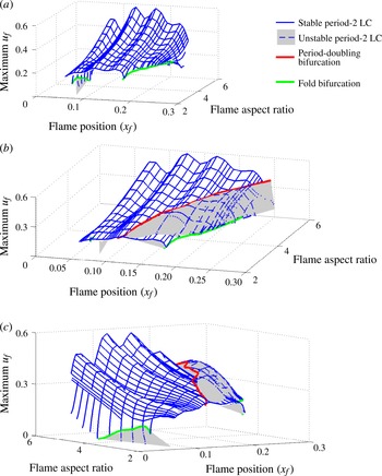
Bifurcation surface of period-2 limit cycles as two parameters are varied: the flame location in the duct,
 $x_{f}$
, and the flame aspect ratio,
 ${\it\beta}$
. The surface is composed of over 1200 limit cycles, each converged to
 $\Vert \boldsymbol{x}(0)-\boldsymbol{x}(T)\Vert <5\times 10^{-4}$
. The surface has regions with unstable limit cycles (dashed blue lines and grey shading) and regions with stable limit cycles (solid blue lines), whose boundaries are defined by the locations of the fold bifurcation (green line) and the period-doubling bifurcation (red line), which is the same as that in figure 5. The unstable limit cycle surface is not shown in (a), but (b) and (c) show the stable and unstable limit cycle surfaces from two different views.

Figure 6 shows the bifurcation surface of period-2 limit cycles, whose frequencies are close to half that of the fundamental acoustic mode. The surface shows the maximum velocity at the flame during the limit cycle. The surface has regions with unstable limit cycles (dashed blue lines and grey shading) and regions with stable limit cycles (solid blue lines), whose boundaries are defined by the locations of the period-doubling bifurcation (red line) and the fold bifurcation (green line). The period-doubling bifurcation is the same as that on the period-1 surface (figure 5). The surface is shown for the same parameter range as figure 5. The fold bifurcation exists at high
 ${\it\beta}$
but its location is unresolved.
Figures 5 and 6 show only the amplitude of the velocity fluctuation during the limit cycles. For the period-2 cycles, more information can be gained by plotting both the peaks and the troughs of the time series during the limit cycle. This is how the experimental results of Kabiraj et al. (Reference Kabiraj, Sujith and Wahi2012b
) and the computational results of Kashinath et al. (Reference Kashinath, Waugh and Juniper2013b
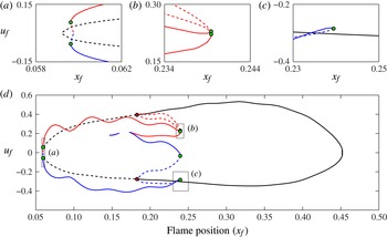
) are presented. Figure 7 shows a two-dimensional slice of the combined period-1 and period-2 bifurcation surfaces, taken at
 ${\it\beta}=4$
, with the vertical axis showing both the peaks and the troughs of the limit cycles.
Two-dimensional slice of the combined period-1 and period-2 bifurcation surfaces, taken at
 ${\it\beta}=4$
. The vertical axis plots the peaks and troughs of the velocity time series: period-1 peaks and troughs are shown in black, period-2 peaks are shown in red and period-2 troughs in blue. Solid lines represent stable limit cycles and dashed lines represent unstable limit cycles. The period-doubling bifurcation is shown as red dots and the fold bifurcations are shown as green dots.

The period-1 cycles (black) have only one peak and one trough and these are not symmetric about zero. The period-2 peaks (red) and period-2 troughs (blue) form a more elaborate shape. At some locations, the period-2 cycles have two peaks and two troughs (
 $0.15<x_{f}<0.16$
,
 $0.17<x_{f}$
), and at other locations the period two cycles have only one peak and one trough (
 $x_{f}<0.15$
,
 $0.16<x_{f}<0.17$
). This difference occurs because the period-2 cycles are composed of two frequencies, whose relative magnitudes change along the period-2 branch (see the next section). As the period-2 branch approaches the period-doubling bifurcation, the two peaks and two troughs close together. The period-doubling bifurcation is subcritical; i.e. the period-2 cycles emerging from it are unstable and overlap with the stable period-1 limit cycle. There is therefore a region of bistability between
 $0.182<x_{f}<0.240$
, where four attractors exist: a stable period-1 limit cycle, a stable period-2 limit cycle, an unstable period-2 limit cycle and an unstable fixed point.
It worth noting that there are only two fold bifurcations on figure 7. The four green dots at
 $x_{f}=0.240$
are not four separate fold bifurcations. They are a single fold bifurcation acting simultaneously on the four separate traces. The same is true of the two green dots at
 $x_{f}=0.06$
.
The period-2 peaks and troughs on figure 7 oscillate with a wavelength of
 ${\rm\Delta}x_{f}=0.1$
, which matches the wavelength of the highest Galerkin mode (20 modes were considered here). These oscillations may be due to an insufficient number of modes in the Galerkin discretisation, or they may due to the Gibbs phenomenon around the flame, which is an inherent problem with the Galerkin discretisation (Sayadi et al.
Reference Sayadi, Le Chenadec, Schmid, Richecoeur and Massot2014). While this makes the amplitude of the limit cycles vary with the flame position, it does not have any influence once the flame position is fixed and could not, for instance, cause the system to trigger from one stable state to another. This is not important for the aims of this paper but is an area to be improved in future studies.
5.2. Limit cycles
Once the limit cycles have been found by the continuation methods, the different types of oscillation can be examined and compared. For example, at a flame position of
 $x_{f}=0.195$
and a flame aspect ratio of 4 (figure 7), there are three limit cycles: a stable period-1 limit cycle, an unstable period-2 limit cycle and a stable period-2 limit cycle, all of which have comparable velocity amplitudes at the flame.
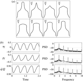
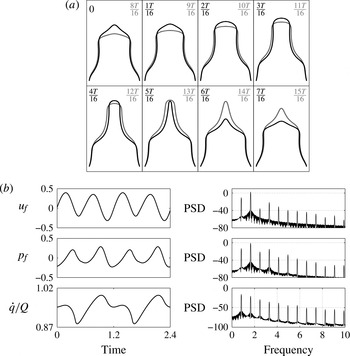
Figure 8(a) shows snapshots of the flame during the stable period-1 limit cycle. These flame shapes are qualitatively similar to those seen in experimental axisymmetric flames (Birbaud et al. Reference Birbaud, Durox and Candel2006). Figure 8(b) shows segments of the time traces and spectra of the acoustic velocity, acoustic pressure and heat release at the flame. The presence of higher harmonics in the spectra, as well as visual inspection of the time traces, shows that none of these signals is harmonic and therefore that an FDF approach would not capture this oscillation accurately.
Snapshots of the flame surface (a) and time traces and spectra (b) for the stable period-1 limit cycle at
 $x_{f}=0.195$
, with steady-state flame aspect ratio of 4.

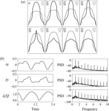
Figure 9 shows the equivalent of figure 8 for the unstable period-2 limit cycle. On the bifurcation diagram, this limit cycle is close to the period-doubling bifurcation and there are clear similarities with the stable period-1 limit cycle. The black lines show the flame shape during the first half of the cycle and the grey lines show the flame shape during the second half of the cycle. Because this is a period-2 limit cycle, a peak appears on the spectra at 0.9, which is half the frequency of the fundamental acoustic mode. Again, this oscillation could not be captured with the FDF approach.
Snapshots of the flame surface (a) and time traces and spectra (b) for the unstable period-2 cycle at
 $x_{f}=0.195$
, with steady state flame aspect ratio of 4. The time scale is the same as figure 8.

Figure 10 shows the equivalent of figures 8 and 9 for the stable period-2 limit cycle. In the spectra, the peak at 0.9, which is half the fundamental frequency, has largest magnitude. On the bifurcation diagram, this limit cycle is further from the period-doubling bifurcation and, without the benefit of continuation analysis, it would be difficult to tell that the cycle is part of the period-2 branch and not simply a limit cycle with half the frequency of the fundamental acoustic mode.
Snapshots of the flame surface (a) and time traces and spectra (b) for the stable period-2 cycle at
 $x_{f}=0.195$
, with steady-state flame aspect ratio of 4. The time scale is the same as figure 8.

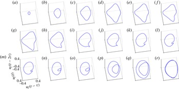
The qualitative change in the form of the cycle along the period-2 branch can be examined using phase portraits. Figure 11 shows the phase portraits of the period-2 cycles at different locations along the period-2 branch of figure 7, starting from near the Hopf bifurcation (figure 11
a) and moving along the branch towards the period-doubling bifurcation (figure 11
r). Near the Hopf bifurcation, the cycle is nearly harmonic with half the frequency of the fundamental mode of the tube. The only indication that this is on the period-2 branch is that it has half the frequency of the fundamental. As
 $x_{f}$
increases, the phase portraits smoothly develop the familiar double-loop, which is characteristic of period doubling. At the bifurcation between period-2 and period-1 limit cycles, the two loops coincide and merge into a single loop. Again, none of this behaviour could be captured with a conventional FDF analysis.
Phase portraits of the period-2 limit cycles at different locations along the period-2 branch of figure 7. Near the Hopf bifurcation (a), the cycle is nearly sinusoidal with a frequency of half the fundamental acoustic mode. The cycle becomes less sinusoidal as
 $x_{f}$
increases (b–h), because the response at the fundamental acoustic mode increases relative to the response at the half-frequency. As the cycle moves closer to the period-doubling bifurcation (i–r) the phase portraits develop the familiar double loop form of a period-2 cycle, because the response of the fundamental acoustic mode is much greater than that of the half-frequency. The fold bifurcation occurs between (o) and ( p); the period-2 cycles (a–o) are stable, the period-2 cycles (p–r) are unstable.

5.3. Bifurcations
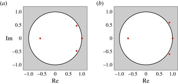
The second aim of this paper is to identify the types of bifurcation by examining the Floquet multipliers of the limit cycles. The Floquet multipliers, which in general are complex numbers, describe the stability of a limit cycle to infinitesimal perturbations. On the one hand, if the magnitudes of all of the Floquet multipliers are less than 1 then all perturbations decay after one cycle and the limit cycle is stable. On the other hand, if the magnitude of at least one Floquet multiplier is greater than 1, then the limit cycle is unstable. The Floquet multipliers are usually represented in the complex plane. In this representation, bifurcations from stable to unstable limit cycles occur when a Floquet multiplier crosses the unit cycle. The location of the crossing point in the complex plane determines the type of bifurcation. In this section, three types of bifurcation are shown: fold bifurcations, period-doubling bifurcations and Neimark–Sacker bifurcations. In all of the figures in this section, the four Floquet multipliers with the largest magnitude are converged to
 $10^{-2}$
accuracy with the Arnoldi algorithm. The Floquet multiplier at
 $(+1,0)$
is the trivial one that defines a limit cycle.
5.3.1. Fold bifurcation
A fold (LPC) bifurcation occurs when a Floquet multiplier crosses the unit circle at
 $(+1,0)$
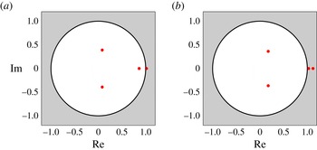
. On the unstable side, infinitesimal perturbations in the direction of the corresponding eigenfunction grow by a constant real factor each cycle. This means that trajectories in phase space spiral away from the limit cycle in a fixed direction at each point around the limit cycle. This continues until the trajectory reaches another attractor. A fold bifurcation is observed on the period-2 branch of figure 7 at
 $x_{f}=0.239$
. Figure 12 shows the Floquet multipliers of the period-2 cycles either side of the fold bifurcation in figure 7. This clearly shows the Floquet multiplier crossing
 $(+1,0)$
. The fold bifurcation at
 $x_{f}=0.239$
and the subcritical period-doubling bifurcation at
 $x_{f}=0.182$
together create a bistable region in which there is a stable period-1 limit cycle and a stable period-2 limit cycle. Mode switching is therefore possible in this parameter regime.
Floquet multipliers either side of the fold bifurcation, at
 $(x_{f},\max (u_{f}))$
values of
 $(0.239,0.224)$
(a) and
 $(0.239,0.244)$
(b) on figure 7. The fold bifurcation is caused by the Floquet multiplier crossing
 $(+1,0)$
. Only the four largest magnitude Floquet multipliers are shown.

5.3.2. Neimark–Sacker bifurcation
A Neimark–Sacker (torus) bifurcation occurs when a complex conjugate pair of Floquet multipliers crosses the unit circle at an angle that is not a simple fraction of
 $2/{\rm\pi}$
. On the unstable side, perturbations in the direction of the corresponding eigenfunction grow by a constant complex factor each cycle. This means that trajectories in phase space spiral away from the limit cycle while also winding around it. This continues until the trajectories reach another attractor, which for a Neimark–Sacker bifurcation is a quasiperiodic attractor. This attractor is an ergodic torus in phase space because the frequency of the motion around one axis of the torus is incommensurate with the frequency of the motion around the other. Figure 13 shows the Floquet multipliers of limit cycles either side of the Neimark–Sacker bifurcation. This clearly show the complex pair of Floquet multipliers crossing the unit circle.
Floquet multipliers either side of the Neimark–Sacker bifurcation on figure 5, at flame aspect ratio of 2.4 and
 $x_{f}$
values of 0.2 (a) and 0.175 (b). The Neimark–Sacker bifurcation is caused by the complex conjugate pair of Floquet multipliers crossing the unit circle.

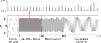
A Neimark–Sacker bifurcation can also be identified from the time series in figure 14. This simulation starts from the unstable limit cycle just after the Neimark–Sacker bifurcation. This unstable limit cycle has one frequency but the perturbations that grow around it have another frequency. The ratio between these two frequencies is given by the argument of the complex eigenvalue pair divided by
 $2{\rm\pi}$
. For the pair of Floquet multipliers in figure 13, the ratio between the two frequencies is 10.57 (to two decimal places). This can be seen in the time series of figure 14, in which the amplitude of the peaks oscillates with a period 10.57 times that of the limit cycle. These perturbations grow exponentially before being attracted to a quasiperiodic attractor whose characteristic incommensurate frequencies are very similar to those of the Niemark–Sacker bifurcation. It is worth noting that if the ratio between the two frequencies is were rational, then the oscillation would be multiperiodic rather than quasiperiodic.
Time series of the system growing exponentially away from an unstable limit cycle just after a Neimark–Sacker bifurcation. The peaks oscillate at a second frequency that is defined by the argument of the pair of Floquet multipliers that cross the unit circle.

5.3.3. Period-doubling bifurcation
A period-doubling (flip) bifurcation occurs when a Floquet multiplier crosses the unit circle at
 $(-1,0)$
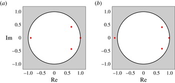
. On the unstable side, infinitesimal perturbations in the direction of the corresponding eigenfunction grow by a constant real factor each cycle but flip from one side to the other of the limit cycle. The bifurcation thereby creates a branch of period-2 limit cycles when the period-1 limit cycle becomes unstable. Figure 15 shows the Floquet multipliers at limit cycles either side of the period-doubling bifurcation in figure 7, which clearly show the Floquet multiplier crossing
 $(-1,0)$
.
Floquet multipliers either side of the period-doubling bifurcation, at
 $x_{f}$
values of 0.193 (a) and 0.175 (b). The period-doubling bifurcation is caused by the Floquet multiplier crossing
 $(-1,0)$
.

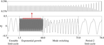
A period-doubling bifurcation can also be identified from the time series in figure 16. This simulation starts from the unstable limit cycle just after the period doubling bifurcation. The perturbation to the limit cycle grows exponentially, which is seen most easily by the exponential growth of the amplitude difference between adjacent peaks. In this case, the unstable limit cycle was converged to a high tolerance and the unstable Floquet multiplier is only just outside the unit circle, so the system requires several oscillations for the exponential growth to become visible.
Time series of the system growing exponentially away from an unstable period-1 limit cycle just after a period-doubling bifurcation. The peaks form a characteristic one-up, one-down pattern. The first and the last boxes have the same scale, to show that the period-2 limit cycle has roughly twice the period of the unstable period-1 limit cycle.

Figure 7 shows that the period doubling bifurcation is subcritical. This means that the exponential growth described above is towards a period-2 limit cycle that is itself unstable. As a consequence, the system rapidly evolves to the stable period-2 limit cycle, as can be seen in the mode switching stage of figure 16.
5.4. Eigenvectors of the Floquet multipliers
The third aim of this paper is to identify the coupled flame–acoustic motion that is responsible for the qualitative change in behaviour at each bifurcation. We do this by analysing the eigenvectors associated with the unstable Floquet multipliers, which we call the Floquet mode. Here, we demonstrate this for the period-doubling bifurcation in § 5.3.3.
At the period-doubling bifurcation, the Floquet mode that corresponds to the Floquet multiplier at
 $(-1,0)$
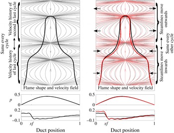
shows which coupled motion of the system is responsible for the bifurcation. This Floquet mode is shown schematically in figure 17. At the frequency of the fundamental acoustic mode, the flame has two cusps on its surface. At half of this frequency, there would be only one cusp. The Floquet mode therefore has a one cusp shape, because the Floquet mode is the perturbation that grows at the half-frequency. The Floquet mode is a coupled motion with: (i) a flapping motion of the flame surface, in which the tip and base of the flame move outwards and the middle of the flame moves inwards, coupled with (ii) a variation in the velocity field every other cycle and (iii) a reduction in the acoustic pressure in the duct and an increase in acoustic velocity in the duct upstream of the flame.
The Floquet mode of the Floquet multiplier that causes the period-doubling bifurcation. The left-hand image shows the flame shape and streamlines of the velocity field at a state on the limit cycle at the period-doubling bifurcation (flame aspect ratio 4). At these limits on the vertical axis, the velocity field in the lower half of the domain is repeated in the upper half of the domain. This is because the velocity field is the history of the acoustic perturbation over the last two cycles; the last cycle corresponds to the lower half of the domain and the second-last cycle corresponds to the upper half of the domain. The left-hand image is copied in grey onto the right-hand image and is superposed in red with the state when perturbed in the direction of the Floquet mode that causes the period-doubling bifurcation. This reveals the coupled motion that is responsible for the period-doubling bifurcation. This is: (i) a flapping motion of the flame surface, in which the tip and base of the flame move outwards and the middle of the flame moves inwards, coupled with (ii) a variation in the velocity field every other cycle and (iii) a reduction in the acoustic pressure in the duct and an increase in the acoustic velocity in the duct before the flame. The flame shape perturbation is scaled by a factor of two for clarity.

It is common practice in thermoacoustics to use linear stability analysis about a fixed point to isolate the frequencies and mode shapes that become unstable at a bifurcation. It is directly analogous to isolate the Floquet multipliers and mode shapes that become unstable at a bifurcation to a limit cycle, and they can therefore be analysed with many of the same techniques. Floquet mode analysis at a bifurcation is therefore useful for several reasons: first, it shows which second frequency becomes part of the oscillation; second, it shows the mode shape of the instability that grows around the limit cycle; third, passive or active control can then be used to suppress this instability in order to move the bifurcation to a more favourable region of parameter space. In the case of a fold bifurcation, the control techniques can therefore shrink regions of bistability where the system is vulnerable to triggering. Further, adjoint techniques can be used to determine the sensitivity of the Floquet multiplier to various control inputs, and therefore to design control systems with optimal controllability.
6. Conclusions
In this paper, matrix-free continuation techniques have been applied to a model of a ducted premixed flame. The flame model uses the kinematic
 $G$
-equation with a local level set solver. The premixed flame model has many attributes of similar experimental systems: the flame is axisymmetric, the flame speed depends on the flame curvature, the flame has sharp cusps and the flame is capable of pinch-off, flashback and bulging at the burner lip. A similar ducted premixed flame model has been shown previously by Kashinath et al. (Reference Kashinath, Waugh and Juniper2013b
) to exhibit limit cycle, period-
 $2^{n}$
, quasiperiodic and chaotic behaviour, and to have many parameter regions that are multistable. These results show qualitatively the same phenomena observed in experiments by Kabiraj et al. (Reference Kabiraj, Sujith and Wahi2012b
).
Continuation techniques are used to efficiently find a surface of stable and unstable limit cycles as two system parameters vary, which was the first aim of this paper. These continuation methods can find unstable limit cycles easily, whereas many other techniques cannot. This is important because the unstable limit cycles are crucial for mode switching (Waugh & Juniper Reference Waugh and Juniper2011; Kashinath et al. Reference Kashinath, Waugh and Juniper2013b ) and for separating the basins of attraction of different attractors. The continuation methods also explicitly find period-doubling and Neimark–Sacker bifurcations by examining the Floquet multipliers of the limit cycles, which was the second aim. These bifurcations and their Floquet multipliers cannot be found with describing function techniques, because they involve the interaction of at least two frequencies, which are not known a priori. A separate surface of period-2 limit cycles was found to emerge from a subcritical period-doubling bifurcation. This is the first computational thermoacoustic study in which period-doubling and Neimark–Sacker bifurcations have been found. The Floquet modes are examined at the bifurcations in order to reveal the coupled flame–acoustic motions that are responsible for the qualitative changes in behaviour, which was the third aim.
The continuation methods shown here converge to each limit cycle by timemarching for only a few cycles. The CPU time to create a bifurcation surface is therefore determined by the time taken to timemarch each cycle. The
 $G$
-equation solver is computationally expensive compared with many simple thermoacoustic models, but despite this, only around 14 000 CPU hours were required to generate the bifurcation surfaces in this paper and to analyse the stability of the limit cycles. This is equivalent to 80 CPU cores running for 1 week. Furthermore, because the surface is composed of several two-dimensional slices, the process of forming a surface is easily parallelisable. For relatively little computational cost, therefore, these continuation methods can characterise the nonlinear behaviour of coupled thermoacoustic systems over a wide parameter range.
The
 $G$
-equation solver used here is able to capture the dynamics of a premixed flame under acoustic forcing. The continuation methods are then able to calculate limit cycles and bifurcations when this flame model is coupled to an acoustic model. The results from these continuation methods could be compared with experiments in one of two ways: first, by comparing flame shapes and heat release responses; second, by comparing the self-excited behaviour and the bifurcation diagrams. With improvements to the velocity model and the acoustic model, the method described in this paper could be an effective means of predicting and analysing the nonlinear behaviour seen in experimental premixed flame systems.
Acknowledgements
I.W. acknowledges the support of EPSRC through a Doctoral Training Grant and the IMechE through the postgraduate scholarship award. K.K. acknowledges the support of EPSRC and Rolls-Royce through a Dorothy Hodgkin studentship. M.J. acknowledges the support of the ERC through project ALORS 2590620.