1. Introduction
This paper presents a new fully nonlinear one-dimensional (1-D) dispersive model for gravity waves over topography in channels with prismatic sections. The model accounts for geometrical dispersion processes appearing in hydrostatic flows, and originating solely by bathymetric variations.
The physical background of this work is the propagation of undular bores in prismatic channels, and can be related to the laboratory experiments by Treske (Reference Treske1994), as well as to the in situ measurements in the Garonne and Seine rivers, reported in Bonneton et al. (Reference Bonneton, Bonneton, Parisot, Sottolichio and Detandt2012, Reference Bonneton, Bonneton, Parisot and Castelle2015). Before the Froude number is high enough for wave breaking to occur (
 $\sim$
1.3), two different dispersive propagation regimes are clearly observable both in laboratory and river experiments. One of them, occurring for Froude numbers higher than
 $\sim$
1.15, corresponds to the usual dispersive undular bore known since the experiments by Favre (Reference Favre1935). These waves are well understood, and can be related theoretically to the classical dispersion relation from Airy theory using the analogy by Lemoine (Reference Lemoine1948). For lower Froude numbers, longer waves are observed which do not correspond to classical dispersive propagation. This phenomenon has been studied in Chassagne et al. (Reference Chassagne, Filippini, Ricchiuto and Bonneton2018, Reference Chassagne, Filippini, Ricchiuto and Bonneton2019) where it has been shown numerically and theoretically that these low-Froude-number undular bores are generated by a purely geometrical process related to refraction in the transverse direction. These waves are unaffected by vertical kinematics, and appear also in hydrostatic flows. So, despite of their dispersive nature, these waves can be simulated using the hyperbolic shallow-water equations as shown in Chassagne et al. (Reference Chassagne, Filippini, Ricchiuto and Bonneton2018, Reference Chassagne, Filippini, Ricchiuto and Bonneton2019). Such a dispersive behaviour of waves in materials with microstructure is well known, see e.g. Berezovski, Engelbrecht & Berezovski (Reference Berezovski, Engelbrecht and Berezovski2011) and Berezovski et al. (Reference Berezovski, Engelbrecht, Salupere, Tamm, Peets and Berezovski2013). Following the asymptotic analysis of Ketcheson & Quezada de Luna (Reference Ketcheson and Quezada de Luna2015) for anisotropic media, in Chassagne et al. (Reference Chassagne, Filippini, Ricchiuto and Bonneton2018, Reference Chassagne, Filippini, Ricchiuto and Bonneton2019) the authors introduce the idea of a scale separation between the characteristic transverse length (
 $\it{l}$
, running across the section) and the characteristic longitudinal length (
 $L$
, in the main propagation direction along the channel axis). Using the smallness of
 $\it{l}/L$
, the authors derive an asymptotic dispersive linear wave equation providing an asymptotic section averaged approximation of the linearised shallow-water system. The dispersion effects, and the dispersion coefficient, depend only on the channel’s geometry. Using the theory by Lemoine (Reference Lemoine1948), the authors use the dispersion relation of their linear model to obtain a good quantitative prediction of the wavelengths of the low-Froude-number waves. These waves are related purely to geometrical effects, and in particular to bathymetric variations. They have been baptised ‘dispersive-like’ in Chassagne et al. (Reference Chassagne, Filippini, Ricchiuto and Bonneton2019). Later on, Quezada de Luna & Ketcheson (Reference Quezada de Luna and Ketcheson2021) used the same formal development to identify solitary waves associated with geometrical dispersion. They also introduce ad-hoc nonlinear terms to obtain heuristic Boussinesq and Korteweg-de Vries (KdV)-like models. Recently, the same averaging procedure has been applied in Ketcheson & Russo (Reference Ketcheson and Russo2024) to the Saint–Venant equations assuming periodic topography and small-amplitude waves.
From the modelling point of view, the first rigorous Boussinesq model for channels with non-rectangular sections dates to the early work by Peregrine (Reference Peregrine1968), focusing on prismatic channels. First generalisations allowing small section variations along the channel axis were proposed by Teng & Wu (1992, 1997). Equations accounting for arbitrary non-uniform cross-sections have been developed in Winckler & Liu (Reference Winckler and Liu2015). All of these models are obtained in a very general setting which starts from the Euler equations and then goes through classical scaling assumptions on length and velocity scales to arrive at models including weak dispersive effects. These scaling hypotheses differentiate between horizontal and vertical motions, and do not account for the differences between transverse and longitudinal horizontal processes. Despite this general setting, it has been shown in Jouy et al. (Reference Jouy, Violeau, Ricchiuto and Le2024) that, for example, the model by Winckler & Liu (Reference Winckler and Liu2015) accounts only for waves associated with geometrical variations, as the linear model by Chassagne et al. (Reference Chassagne, Filippini, Ricchiuto and Bonneton2019). There is thus some ambiguity on which type of dispersion is modelled by existing equations, and which range of applications they can be used for.
Here we propose a 1-D fully nonlinear model for dispersive-like waves originating from two-dimensional (2-D) bathymetric variations. In this respect, the present work is inherently different from previous work on section averaged dispersive models. There is no ambiguity on the dispersive process modelled, which is relying fully on horizontal kinematics. The new geometrical Green–Naghdi (gGN) model proposed is derived from the nonlinear hyperbolic shallow-water equations. We call this model the Green–Naghdi (GN) type (and not, as conventionally, the Serre–Green–Naghdi type or SGN) to emphasise that it is based on the model taking into account the effects of 2-D bathymetry. The physical assumptions made are somewhat similar to those invoked in Chassagne et al. (Reference Chassagne, Filippini, Ricchiuto and Bonneton2019), albeit retaining the full hydrodynamic nonlinearity. The new section averaged gGN model is thus fully nonlinear, it has a Lagrangian structure, and, as a consequence, an exact energy conservation law. We study the propagation properties of the model, and show the existence of several types of exact travelling-wave solutions including solitary waves and periodic waves. We propose two reformulations to solve the partial differential equation (PDE) system numerically: the first based on a elliptic–hyperbolic decomposition Filippini, Kazolea & Ricchiuto (Reference Filippini, Kazolea and Ricchiuto2016), the second using a hyperbolic relaxation approach Favrie & Gavrilyuk (Reference Favrie and Gavrilyuk2017). We discuss the numerical approximation of both formulations, and provide a thorough investigation of the model, which is validated both using comparisons with transverse averages of full 2-D shallow-water simulations, and against the experiments by Treske (Reference Treske1994) in the low-Froude-number range.
The structure of the paper is as follows. In § 2 we introduce the asymptotic hypothesis and discuss the formal derivation of the model. Section 3 is devoted to the study of some of its properties: energy conservation law, dispersion relation, travelling-wave solutions. In § 4 we propose some reformulations of the system more suitable for its numerical approximation. In § 5 we validate the model by comparing it with averaged 2-D shallow-water computations, as well as with experiments in prismatic channels with a trapezoidal cross-section. Additional technical details related to the model and numerical methods are given in the Appendices.
2. Equations averaged in
 $y$
-direction

We consider shallow-water flows over topography described by the classical 2-D Saint–Venant equations:
 \begin{align} h_t +(hu)_x+(hv)_y &=0, \end{align}
 \begin{align} (hu)_t + \left(hu^2+g \dfrac{h^2}{2} \right)_x+(huv)_y &=-gh b_x, \end{align}
 \begin{align} (hv)_t +(huv)_x + \left(hu^2+g \dfrac{h^2}{2} \right)_y &=-gh b_y. \end{align}
Here
 $t$
is time,
 $(x,y)$
are the Cartesian coordinates, respectively, running in the longitudinal (channel axis,
 $x$
) and transverse (across the sections,
 $y$
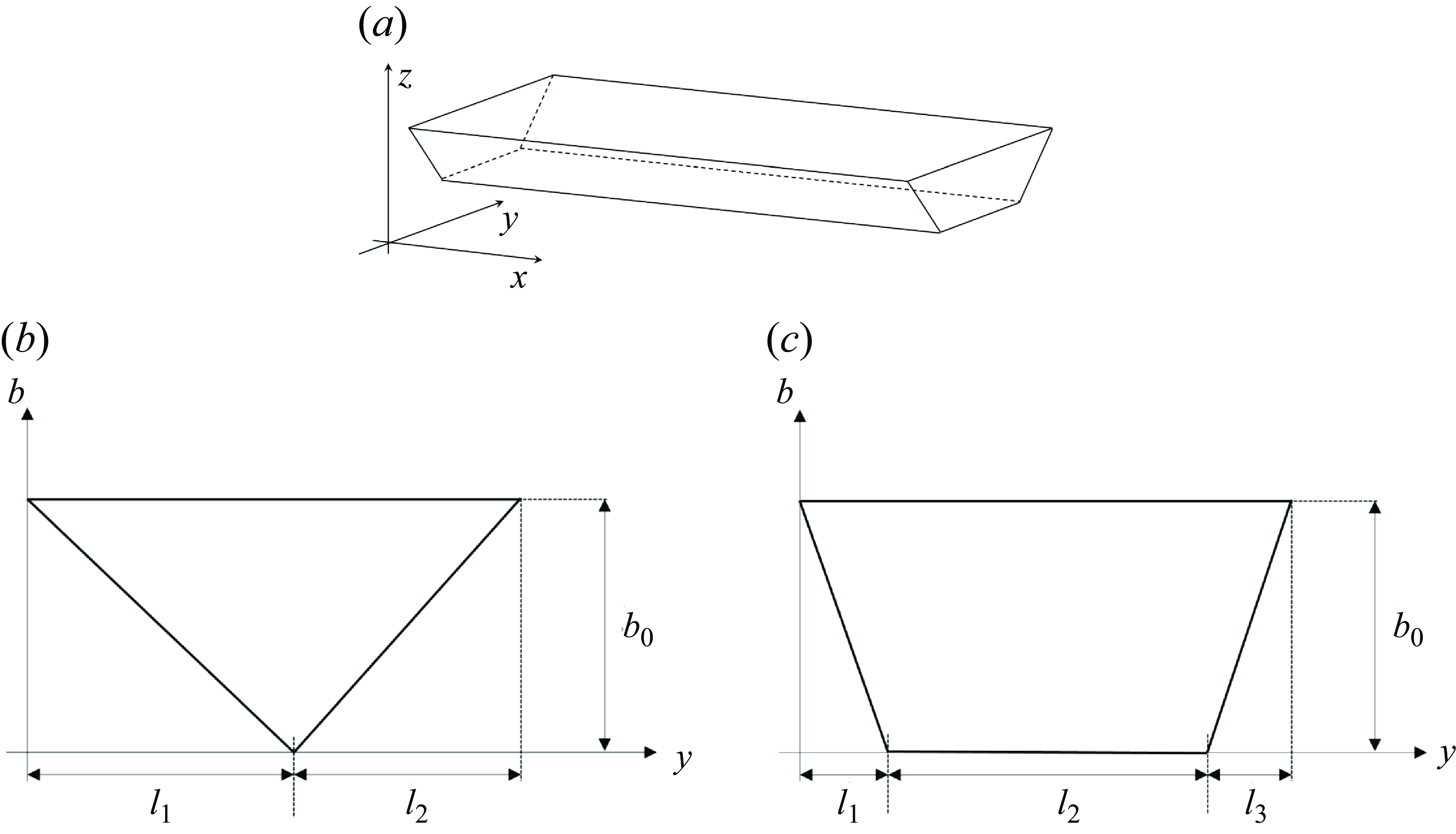
) directions (see the sketch in figure 1
a). We denote by
 $h$
the fluid depth,
 $(u,v)$
the
 $x$
- and
 $y$
-velocity components,
 $b(x,y)$
is the bottom topography, and
 $g$
is the acceleration of gravity.
We assume that the transverse and longitudinal propagation processes are characterised by two different length scales
 $\textit {l}$
and
 $L$
, respectively, such that
 $\textit { l} \ll L$
. We thus introduce the small parameter
 \begin{equation} \varepsilon:= \dfrac {l}{L}. \end{equation}
Let
 $H$
be the characteristic vertical length, usually taken as the characteristic undisturbed water depth, see e.g. Peregrine (Reference Peregrine1968). We introduce the following dimensionless variables (denoted with the ‘tilde’ sign):
 \begin{align} x=L\tilde x, \; y=\varepsilon L\; \tilde y, \; t=L/\sqrt {gH} \; \tilde t, \; u=\sqrt {gH}\; \tilde u, \; v=\varepsilon \sqrt {gH}\; \tilde v, \end{align}
 \begin{align} h=H\; \tilde h, \; b=H\; {\tilde b}. \end{align}
Introducing this scaling in the equations, and suppressing for simplicity the ‘tilde’, we can write the dimensionless system as follows:
 \begin{align} h_t +(hu)_x+(hv)_y &=0, \end{align}
 \begin{align} (hu)_t +\left (hu^2+\frac {h^2}{2}\right)_x +(huv)_y+hb_x &=0, \end{align}
 \begin{align} \varepsilon ^2(v_t +uv_x+vv_y)+(h+b)_y & =0. \end{align}
Note that the equation for
 $v$
is written in non-conservative form for later convenience. We now introduce some of our main hypotheses.
The first is that the channel has a prismatic bathymetry defined as
 $b=b(y)$
. A slow variation of
 $b$
with
 $x$
could also be included, for example
 $\partial _x b=\mathcal{O}(\varepsilon ^\beta)$
for some
 $\beta \gt 0$
. We will leave this out for simplicity.
The second important hypothesis is that
 $(hv)\big |_{y=0}=(hv)\big |_{y=l}$
and
 $(hvu)\big |_{y=0}=(hvu)\big |_{y=l}$
. Note that these two conditions are equivalent for flows in channels with banks (
 $h=0$
on both sides), as well as in channels with reflective straight walls (
 $v=0$
on both sides). They are obviously satisfied for flows which are
 $l$
-periodic in the
 $y$
-direction, with an
 $l$
-periodic bathymetry:
 $b(y)=b(l+y)$
.
Our aim is to replace the 2-D equations with an equivalent system of averaged 1-D equations, which exhibit dispersive behaviour similar to that of the original model. To this end we will average (2.5) in the transverse direction across a length
 $\it{l}$
, which we assume to be constant. This length can be a given channel width (for channels with vertical walls), or the width of a reference/initial wet section, or the period in the case of periodic topography. Figures 1(b) and 1(c) show typical geometries encountered in practice, and give some initial notation.
Channel geometry: (a) longitudinal axis
 $x$
, transverse axis
 $y$
, vertical axis
 $z$
; (b) triangular section with
 ${ l}={ l}_1+{ l}_2$
, and
 $b(0)=b({ l})=b_0, \; b({ l}_1)=0$
; (c) trapezoidal section with
 ${ l}={ l}_1 + { l}_2 +{ l}_3$
and
 $b(0)=b({ l})=b_0, \; b({ l}_1)= b({ l}_1+{ l}_2)=0$
.

2.1. Generalities and asymptotic expansion
For any function
 $f(t,x,y)$
, we will use two types of averaging operators in the
 $y$
-direction. One is standard:
 \begin{equation} \overline {f}(t,x)=\frac {1}{l}\int _0^{l}f(t,x,y)\text{d}y. \end{equation}
The second one defines the weighted averaged value:
 \begin{equation} \langle f\rangle =\frac {1}{l\overline {h}}\int _0^{l}h(t,x,y)f(t,x,y)\text{d}y. \end{equation}
Sometimes the last averaging is called Favre averaging. The advantage of definition (2.7) is that the mass conservation law is exactly satisfied in the usual sense, with the velocity
 $\langle u\rangle$
. The dimensionless averaged conservative form of equations (2.1a
), (2.1b
) in the case
 $b=b(y)$
becomes
 \begin{align} &\overline {h}_t +(\overline {h}\langle u\rangle)_x =0, \end{align}
 \begin{align} &(\overline {h}\langle u\rangle)_t +\left(\overline {hu^2}+\frac {1}{2}\overline {h^2}\right)_x=0. \end{align}
We need to find
 $\overline {hu^2}$
and
 $\overline {h^2}$
. Equation (2.5c
) implies
 \begin{equation} h+b=\overline {h}+\overline {b}+{\mathcal {O}}(\varepsilon ^2). \end{equation}
We want to find this
 $ {\mathcal {O}}(\varepsilon ^2)$
term in (2.9) in explicit form. For this, we make the following ansatz for the velocity
 $u$
in
 $x$
-direction:
 \begin{equation} u(t,x,y)= \langle u\rangle (t,x)+{\mathcal {O}}(\varepsilon ^2). \end{equation}
This ansatz means that the shear effects of
 $u$
in the
 $y$
-direction are negligible, i.e. the velocity in the
 $x$
-direction is almost
 $y$
-independent (see Michel-Dansac, Noble & Vila (Reference Michel-Dansac, Noble and Vila2021) for the derivation of a model for fluid flows in prismatic channels with shear effects, but without dispersive effects). The ansatz (2.10) can be considered as a potential flow assumption commonly used for the derivation of the Saint–Venant equations. Indeed, the equations (2.5a
)–(2.5c
) imply the dimensionless vorticity equation in the form
 \begin{align} \frac {D}{Dt}\left (\frac {\omega }{h}\right) =0, \quad \frac {D}{Dt}=\frac {\partial }{\partial t} +u\frac {\partial }{\partial x} +v\frac {\partial }{\partial y}, \quad \omega = \varepsilon ^2 v_x-u_y. \end{align}
If
 $\omega =0$
initially, it stays zero for any time. Integrating the equation
 $\omega =0$
with respect to
 $y$
, we have
 \begin{align} u(t,x,y)=c(t,x)+\varepsilon ^2 \int _0^y v_x(t,x,s)\text{d}s, \end{align}
where
 $c(t,x)$
is the integration constant. Multiplying this expression by
 $h$
, one obtains
 \begin{align} h(t,x,y)\, u(t,x,y)=h(t,x,y)\,c(t,x)+\varepsilon ^2 h(t,x,y)\,\int _0^y v_x(t,x,s)\text{d}s. \end{align}
The averaging with respect to
 $y$
then gives
 \begin{align} c(t,x)= \langle u \rangle (t,x)+{\mathcal O}(\varepsilon ^2) \end{align}
and
 \begin{align} u- \langle u \rangle ={\mathcal O}(\varepsilon ^2). \end{align}
Also,
 \begin{align} \overline {hu^2}=\overline {h(u- \langle u \rangle + \langle u \rangle)^2}=\overline {h(u- \langle u \rangle)^2}+ 2\overline {h(u- \langle u \rangle)}\, \langle u \rangle +\overline {h}\langle u \rangle ^2 \nonumber \\ =\overline {h(u- \langle u \rangle)^2}+\overline {h} \langle u \rangle ^2=\overline {h} \langle u \rangle ^2+{\mathcal {O}}(\varepsilon ^4). \end{align}
An additional hypothesis about the behaviour of
 $v$
will be now specified. Replacing ansatz (2.10) into the mass conservation law (2.5a
), one obtains for
 $v$
the equation
 \begin{equation} \overline {h}_t+((\overline {h}+\overline {b}-b)\langle u \rangle)_x+ (hv)_y={\mathcal {O}}{(\varepsilon ^2)}. \end{equation}
Since
 \begin{align} \overline {h}_t+(\overline {h}\langle u \rangle)_x=0, \end{align}
one gets
 \begin{align} (\langle u \rangle (\overline {b}-b))_x+ (hv)_y={\mathcal {O}}{(\varepsilon ^2)}. \end{align}
Integration with respect to
 $y$
implies:
 \begin{align} { hv}=C(t,x)- S(y)\; \langle u \rangle _x +{\mathcal {O}}{(\varepsilon ^2)}, \quad S(y)= \int _0^y(\overline {b}-b(y^{\prime})) \text{d}y^{\prime}. \end{align}
The function
 $S(y)$
plays an important role in this work. It has the property
 $S(0)=S(\textit{l})=0$
. Moreover we prove in Appendix A that in the case
 $b(y)=b(l-y)$
for any
 $0\lt y\lt l$
, i.e.
 $b(y)$
symmetric with respect to the channel axis, we have
 $\bar S=0$
. We will see the importance of this result shortly.
Concerning the integration ‘constant’
 $C(t,x)$
, we need to determine it using additional hypotheses. For the applications we have in mind (flow in prismatic channels), we use the requirement of a vanishing average discharge in the
 $y$
-direction:
 \begin{align} \int _{0}^{l}hv \text{d}y=0, \end{align}
which leads to
 $C(t,x)=\overline {S}\; \langle u \rangle _x+{\mathcal {O}}{(\varepsilon ^2)}$
.
2.2. Small-scale geometrical effects on the section averaged flow
Using the earlier results, we can now write the asymptotic formula for
 $v$
:
 \begin{equation} { hv =(\overline {S}- S(y))\; \langle u \rangle _x+{\mathcal {O}}{(\varepsilon ^2)}}. \end{equation}
If
 $\overline {S}=0$
, then, due to the property
 $S(0)=S(l)=0$
, the vanishing transverse flow discharge directly implies the smallness of the transverse velocities:
 $v(t,x,0)={\mathcal {O}}{(\varepsilon ^2)}$
and
 $v(t,x,l)={\mathcal {O}}{(\varepsilon ^2)}$
. This justifies, in particular, the application of the averaged model to flows in prismatic channels with vertical walls. Equation (2.22) and mass conservation (2.8a
) combined to give the following expression for the transverse velocity (
 ${\mathcal {O}}{(\varepsilon ^2)}$
error will not be indicated and replace by the sign
 $\approx$
):
 \begin{equation} v(t,x,y)\approx \frac {(\overline {S}- S(y)) }{\overline {h}+S_y}\; \langle u \rangle _x=\frac {(\overline {S}- S(y))\dot \tau }{1+\tau S_y}, \end{equation}
with
 $\tau =1/{\overline {h}}$
, and the ‘dot’ denotes the total derivative along the longitudinal direction
 \begin{equation} \dot {\tau } =\frac {\partial \tau }{\partial t}+\langle u \rangle \frac {\partial \tau }{\partial x}. \end{equation}
We set
 \begin{equation} \sigma (y) = \overline {S}-S(y). \end{equation}
The function
 $\sigma (y)$
has the following properties:
 \begin{equation} \sigma (0)=\sigma (l)=\overline {S}, \quad \overline {\sigma }=0,\quad \frac {\text{d}\sigma }{\text{d}y} = b(y) - \bar b,\quad \quad \overline {\frac {\text{d}\sigma }{\text{d}y}} =0. \end{equation}
We can thus write the following approximation for
 $v$
:
 \begin{equation} v(t,x,y)\approx \frac {\sigma (y) \dot {\tau }(t,x)}{\displaystyle 1-\tau (t,x) \frac {\text{d} \sigma (y)}{\text{d}y}}. \end{equation}
We are now able to find the
 ${\mathcal O}(\varepsilon ^2)$
terms from (2.5c
):
 \begin{equation} (h+b)_y=-\varepsilon ^2(v_t+uv_x+vv_y)+{\mathcal {O}}(\varepsilon ^4)=-\varepsilon ^2\left (\dot {v} +v v _y\right)+{\mathcal {O}}(\varepsilon ^4). \end{equation}
One has
 \begin{equation} \dot {v}(t,x,y)\approx \frac {\sigma \ddot {\tau }}{\displaystyle 1-\tau \frac {\text{d} \sigma }{\text{d}y}}+\frac {\sigma \displaystyle \frac {\text{d} \sigma }{\text{d}y}\dot {\tau }^2}{\left (\displaystyle 1-\tau \frac {\text{d} \sigma }{\text{d}y}\right)^2}, \end{equation}
and
 \begin{equation} h+b= \overline h+\overline b-\varepsilon ^2 \left ( M-\overline M\right)+\mathcal{O}(\varepsilon ^4), \quad M(t,x,y)= \int _0^y \dot {v}\left (t,x,s \right)\text{d}s+\frac {v^2 (t,x,y)}{2}. \end{equation}
Or
 \begin{equation} h= \overline {h}-\frac {\text{d}\sigma }{\text{d}y}-\varepsilon ^2 \left ( M-\overline M\right)+{\mathcal {O}}(\varepsilon ^4). \end{equation}
Thus
 \begin{equation} \overline {h^2}=\overline {\left (\overline {h}-\frac {\text{d}\sigma }{\text{d}y}\right)^2}-2\varepsilon ^2 \overline {\left (\overline {h}-\frac {\text{d}\sigma }{\text{d}y}\right)\left (M-\overline {M}\right)}+{\mathcal {O}}(\varepsilon ^4) \end{equation}
 \begin{equation} =\overline {h}^2+2\varepsilon ^2 \overline {M\, \frac {\text{d}\sigma }{\text{d}y}}+const+{\mathcal {O}}(\varepsilon ^4), \end{equation}
because
 $\displaystyle \overline {{(\text{d}\sigma)}/{(\text{d}y)}}=0$
. From this we can deduce that within
 ${\mathcal {O}}(\varepsilon ^4)$
 \begin{equation} \left (\dfrac {\overline {h^2}}{2}\right)_x= \left ( \dfrac {\overline {h}^2}{2} \right)_x+ \varepsilon ^2 \left (\overline {M\, \frac {\text{d}\sigma }{\text{d}y}}\right)_x, \end{equation}
where the general expression for
 $M$
is
 \begin{equation} M=\int _0^y\left (\frac {\sigma (s) \ddot {\tau }}{\displaystyle 1-\tau \frac {\text{d} \sigma (s)}{\text{d}s}}+\frac {\sigma (s)\displaystyle \frac {\text{d}\sigma (s)}{\text{d}s}\dot {\tau }^2}{\left (\displaystyle 1-\tau \frac {\text{d} \sigma }{\text{d}s}\right)^2}\right)\text{d}s+\frac {\sigma ^2(y) \dot {\tau }^2}{2\left (\displaystyle 1-\tau \frac {\text{d} \sigma }{\text{d}y}\right)^2}. \end{equation}
Note that the denominator
 $ 1- \tau ({(\text{d} \sigma)}/{(\text{d}y)})= 1 -(b(y) - \bar b)/\bar h$
can be easily shown to be strictly positive for many sections of practical relevance, e.g. trapezoidal ones.
We introduce two important particular cases, and then will devote the paper to the in-depth study of one of them. We first consider channels verifying the assumption
 $\overline {S}=0$
which is, in particular, satisfied for symmetric channel cross-sections (see Appendix A for a proof). Formally, since only
 ${\mathcal{O}}(\varepsilon ^2)$
terms are retained in the equations, this assumption can be weakened to
 $\overline {S}={\mathcal{O}}(\varepsilon ^\beta)$
, with
 $\beta \gt 0$
. In this case, one could speak of quasisymmetric channel cross-sections. This first family of models can be characterised by the following property.
Proposition 1 (Lagrangian structure for symmetric and quasisymmetric channel cross-sections). Consider quasisymmetric channel cross-sections for which
 $\bar S = {\mathcal O}(\varepsilon ^\beta)$
with
 $\beta \gt 0$
. Then, up to terms of order
 $ {\mathcal O}(\varepsilon ^{\beta })$
, the term
 $\displaystyle \overline {M\, ({(\text{d}\sigma)}/{(\text{d}y)})}$
can be written as the variational derivative of the Lagrangian potential:
 \begin{align} {\mathcal {L}}(\tau, \dot \tau)=\overline {N\frac {\text{d}\sigma }{\text{d}y}} \end{align}
with
 \begin{equation} N(\tau,\dot \tau,y)=\frac {\dot \tau ^2}{2}\int _{0}^{y}\frac {\sigma (s)\text{d}s}{1-\displaystyle \tau \frac {\text{d}\sigma }{\text{d}s}}. \end{equation}
More precisely, we have
 \begin{equation} \overline {M\frac {\text{d}\sigma }{\text{d}y}}=-\left (\frac {\partial {\mathcal {L}}}{\partial \tau }-\frac {D}{Dt}\left (\frac {\partial {\mathcal {L}}}{\partial \dot \tau }\right)\right) +{\mathcal O}(\varepsilon ^{\beta }). \end{equation}
For symmetric channel cross-sections verifying the condition
 $\bar S=0$
, (2.38) is exact (the term
 ${\mathcal O}(\varepsilon ^{\beta })$
identically vanishes).
The proof is given in Appendix B.
Proposition 1 shows that for quasisymmetric channel cross-sections the pressure term in our model has a Lagrangian structure:
 \begin{equation} \frac {\overline {h^2}}{2}\approx \frac {(\overline {h})^2}{2}-\varepsilon ^2\frac {\delta {\mathcal L}}{\delta \tau }, \quad \textrm { with} \quad \frac {\delta {\mathcal L}}{\delta \tau }=\frac {\partial {\mathcal {L}}}{\partial \tau }-\frac {D}{Dt}\left (\frac {\partial {\mathcal {L}}}{\partial \dot \tau }\right). \end{equation}
We call this model symmetric gGN equations. The advantage of the formulation (2.39) are multiple. In particular, the form (2.39) guarantees the variational formulation of our equations (Gavrilyuk Reference Gavrilyuk2011), and, as a consequence, the existence of an exact energy balance law. More details are given in the next section.
This derivation provides a large family of models. Its form, however, does not allow closed-form expressions for the dispersion coefficients. To obtain some simplification, we consider a different geometrical ansatz. As we have already mentioned, the condition
 $1 - \displaystyle \tau ({(\text{d}\sigma)}/{(\text{d}y)}) \gt 0$
can be easily shown for sections of practical importance. An interesting limit is obtained when considering channels which are wide compared with the depth. This is typically the case in realistic applications both in natural and artificial environments. For this case, we can assume further that the ratio
 $\displaystyle \tau{((\text{d}\sigma)}{(\text{d}y))}$
is small, namely
 $\displaystyle \tau {((\text{d}\sigma)}/{(\text{d}y))}=\mathcal{O}(\epsilon ^{\gamma })$
for some
 $\gamma \gt 0$
. In this case, one can easily show that
 \begin{align} M = \int _0^y\left (\sigma (s) \ddot {\tau }+\sigma (s)\displaystyle \frac {\text{d}\sigma (s)}{\text{d}s}\dot {\tau }^2\,\right)\text{d}s+\frac {\sigma ^2(y)}{2}\dot {\tau ^2} + \mathcal{O}(\epsilon ^{\gamma }). \end{align}
Neglecting the asymptotically small
 $\mathcal{O}(\epsilon ^{\gamma })$
term, we obtain
 \begin{align} M\approx \ddot {\tau }\int _0^y\sigma (s)\text{d}s+\sigma ^2(y)\dot \tau ^2-\dot \tau ^2\frac {\sigma ^2(0)}{2}. \end{align}
Hence,
 \begin{equation} \overline {\frac {\text{d}\sigma }{\text{d}y} M}=\ddot {\tau }\overline { \frac {\text{d}\sigma }{\text{d}y}\int _0^y\sigma (s)\text{d}s}= \ddot {\tau }\left (\overline {\frac {d}{\text{d}y}\left (\sigma (y)\int _0^y\sigma (s)\text{d}s\right)-\sigma ^2}\right) \end{equation}
 \begin{equation} =\ddot {\tau }\left (\sigma (l) \overline {\sigma }-\overline {\sigma ^2}\right) =-\ddot {\tau }\overline {\sigma ^2} =-\chi \ddot {\tau }, \quad \textrm { with }\quad \quad \chi =\overline {S^2}-\overline {S}^2\gt 0. \end{equation}
This limit also enjoys a very important structural property, which can be formulated in the following way.
Proposition 2 (Lagrangian structure for wide channel cross-sections). Consider wide channels for which
 $\displaystyle \tau{((\text{d}\sigma)}/{(\text{d}y))}=\mathcal{O}(\epsilon ^{\gamma })$
, with
 $\gamma \gt 0$
. Then, up to terms of order
 $ {\mathcal O}(\varepsilon ^{\gamma })$
, the hydrodynamic term
 $\displaystyle \overline {M\, {((\text{d}\sigma)}/{(\text{d}y))}}$
can be written as the variational derivative of a Lagrangian potential. More precisely, we have
 \begin{equation} \overline {M\frac {\text{d}\sigma }{\text{d}y}}=-\left (\frac {\partial {\mathcal {L}}}{\partial \tau }-\frac {D}{Dt}\left (\frac {\partial {\mathcal {L}}}{\partial \dot \tau }\right)\right) +{\mathcal O}(\varepsilon ^{\gamma }) \end{equation}
with
 \begin{equation} {\mathcal {L}}(\tau, \dot \tau)= -\chi \, \frac {\dot \tau ^2}{2}. \end{equation}
and
 $\chi$
as in (2.43).
We will refer to the last model, having a very simple form, as simplified gGN equations. We will devote the remainder of the paper to the study of its theoretical properties, and to its applications to the propagation of undular bores in channels.
The simplified gGN model can be considered as a prototype averaged model, containing only one (geometrical) parameter
 $\chi$
. In the case of symmetric channel cross-sections,
 $ \chi =\overline {S^2}$
.
For the prototype average model, (2.8a )–(2.8b ) can be written in dimensional variables as follows:
 \begin{align} \overline {h}_t +(\overline {h}\langle u\rangle)_x =0, \end{align}
 \begin{align} &(\overline {h}\langle u\rangle)_t + \left(\overline {h}\langle u\rangle ^2+ g \frac {\overline {h}^2}{2} + p\right)_x=0, \end{align}
where we set
 \begin{equation} p = -\chi \ddot \tau, \quad \tau =\dfrac {1}{\overline h}, \quad \chi =\overline {S^2}-\overline {S}^2\gt 0, \end{equation}
with
 $ \chi$
having dimension
 $[m^4]$
.
2.3. Expressions for the geometric parameter for the triangular and trapezoidal sections
The value of the parameter
 $\chi$
for a triangular-type bottom (see figure 1
b) is
 \begin{equation} \chi =\frac {b_0^2\big({l}_1^2+4{l}_1{l}_2+{l}_2^2\big)}{720}. \end{equation}
Here
 $b_0$
is the bottom height (
 $b_0=b(0)=b(l)$
), and
 ${l}_1$
is the position of the bottom singularity (
 $b({l}_1)=0$
, and
 ${ l}={ l}_1+{ l}_2$
). The value of the parameter
 $\chi$
for a trapezoidal type bottom is
 \begin{equation} \chi =\frac {b_0^2\big({l}_1+{l}_3\big)\big({l}_1^3+{l}_1^2\big(6{l}_2+5{ l}_3\big)+{ l}_3(15{ l}_2^2+6{ l}_2{ l}_3+{ l}_3^2)+{ l}_1\big(15{ l}_2^2+24{ l}_2{ l}_3+5{ l}_3^2\big)\big)}{720({ l}_1+{ l}_2+{ l}_3)^2}. \end{equation}
Here
 $b_0$
is the bottom height (
 $b_0=b(0)=b(l)$
),
 ${ l}_1$
is the position of the first bottom singularity (
 $b({ l}_1)=0$
),
 ${ l}_1+{ l}_2$
is the position of the second bottom singularity (
 $b({ l}_1+{ l}_2)=0$
),
 $b(y)=0$
for
 $y\in ({ l}_1, { l}_1+{ l}_2)$
, and
 ${ l}={ l}_1+{ l}_2+{ l}_3$
.
The formulas coincide if one takes
 ${ l}_2=0$
and replaces
 ${ l}_3$
by
 ${ l}_2$
. Moreover, formulas (2.49) and (2.50) are symmetric with respect to the pairs (
 ${ l}_1,\,{ l}_2$
) and (
 ${ l}_1,\,{ l}_3$
), respectively. This implies that the dispersion effects are insensitive to mirroring of asymmetric shapes, as one should expect. Similarly, one easily verifies that asymmetric configurations have a smaller dispersion coefficient than symmetric ones. For this, one has to look for the minimum of
 $\chi$
under the constraint
 $l_1+l_2=l$
in the case of the triangular-type bottom, or under the constraint
 $l_1+l_2+l_3=l$
in the case of trapezoidal-type bottom. For the triangular bottom topography, the maximal value of
 $\chi /(b_0^2 l^2)$
is achieved for
 $l_1=l_2=l/2$
, and is approximately equal to
 $0.002\,0833$
. For the trapezoidal bottom, the maximal value of
 $\chi /b_0^2l^2$
is achieved for
 $\displaystyle l_1=l_3=(21-\sqrt {41}) l/40$
, and is approximately equal to
 $0.002\,7139$
.
3. Properties of the gGN-type system
3.1. Galilean invariance
The geometrical models obtained in the previous section can be formally written as
 \begin{align} \begin{aligned} \dot {\bar h} +& \bar h \langle u\rangle _x =0, \\ \bar h \dot { \langle u\rangle } +& g\bar h \bar h_x + p(\tau,\dot \tau,\ddot \tau)_x=0, \quad p=-\left(\frac{\partial {\mathcal{L}}}{\partial \tau}-\frac{D}{Dt}\left(\frac{\partial {\mathcal{L}}}{\partial \dot{\tau}}\right)\right),\end{aligned} \end{align}
These equations involve only a space derivative and first and second 1-D material time derivatives (denoted, as usual, by a ‘dot’). Now, consider a Galilean reference frame moving with a constant velocity. Both space and material time derivatives are invariant with respect to this change of the reference frame. Thus, the model is Galilean invariant.
3.2. Lagrangian structure and energy equation
Consider the Hamilton action
 \begin{equation} a=\int _{t_0}^{t_1}\; L\; \text{d}t,\quad L=\int _{-\infty }^{+\infty }\left (\overline {h}\frac {\langle u\rangle ^2}{2}-W(\overline {h}, \dot {\overline {h}})\right)\text{d}x, \quad W(\overline {h}, \dot {\overline {h}})=\overline {h}\, w(\overline h, \dot {\overline h}). \end{equation}
Here
 $t_i$
,
 $i=0,1$
, are given time instants, and
 $w(\overline h, \dot {\overline h})$
is a given potential. The mass conservation law
 \begin{align} \overline {h}_t +(\overline {h}\langle u\rangle)_x =0 \end{align}
is considered as a differential constraint. Then, the Euler–Lagrange equation (momentum equation) for (3.2) can be written as (see e.g. Gavrilyuk Reference Gavrilyuk2011; Tkachenko, Gavrilyuk & Massoni Reference Tkachenko, Gavrilyuk and Massoni2023)
 \begin{align} \left (\overline {h}\langle u\rangle \right)_t +\left (\overline {h}\langle u\rangle ^2+\overline {h}^2\frac {\delta w}{\delta \overline {h}}\right)_x =0, \quad \textrm { with}\quad \frac {\delta w}{\delta \overline {h}}=\frac {\partial w}{\partial \overline {h}}-\frac {D}{Dt}\left (\frac {\partial w}{\partial \dot {\overline h}}\right). \end{align}
Introducing a new potential
 ${\tilde w}(\tau,\dot \tau)$
as
 \begin{align} \tilde {w}(\tau, \dot {\tau })=\tilde {w}\left (\frac {1}{\overline {h}}, - \frac {\dot {\overline {h}}}{\overline {h}^2}\right)=w(\overline {h}, \dot {\overline {h}}), \end{align}
one can also rewrite the momentum equation in the form
 \begin{align} \left (\overline {h}\langle u\rangle \right)_t +\left (\overline {h}\langle u\rangle ^2-\frac {\delta \tilde w}{\delta \tau }\right)_x =0, \quad \textrm { with}\quad \frac {\delta \tilde {w}}{\delta \tau }=\frac {\partial \tilde {w}}{\partial {\tau }}-\frac {D}{Dt}\left (\frac {\partial \tilde {w}}{\partial \dot {\tau }}\right). \end{align}
where
 $\delta w/\delta \tau$
denotes the variational derivative of
 $w$
. Thus, the averaged equations in the transverse direction both for the symmetrical case and the simplified case are obtained by taking
 \begin{align} \tilde w(\tau, \dot \tau)=\frac {g}{2\tau }+ {\mathcal L}(\tau, \dot \tau). \end{align}
Setting
 $ \bar q = \overline {h}\langle u\rangle$
, the system admits the energy conservation law which is a consequence of invariance of the Lagrangian under time shift:
 \begin{equation} \left (\overline {h}\left (\frac {\langle u\rangle ^2}{2}+g\frac {\overline h}{2}+E\right)\right)_t +\left (\overline {q} \left (\frac {\langle u\rangle ^2}{2}+g\frac {\overline h}{2}+E\right) + \left (g\frac {\overline {h}^2}{2}- \frac {\delta \mathcal L}{\delta \tau }\right) \langle u\rangle \right)_x=0, \end{equation}
with
 \begin{align} E= {\mathcal L}-\dot {\tau }\frac {\partial \mathcal L}{\partial \dot \tau }. \end{align}
In particular, for model (2.46)–(2.47)–(2.48) we have
 \begin{equation} \left (\overline {h}\left (\frac {\langle u\rangle ^2}{2}+ g\frac {\overline h}{2}+\frac { \chi \dot \tau ^2}{2}\right)\right)_t +\left (\overline {q} \left (\frac {\langle u\rangle ^2}{2}+g\frac {\overline h}{2}+\frac { \chi \dot \tau ^2}{2}\right) + \left (g\frac {\overline {h}^2}{2}- \chi \ddot \tau \right) \langle u\rangle \right)_x=0. \end{equation}
3.3. Linear dispersion properties
Consider now the linearised version of (2.46), (2.47) and (2.48) on a flow at rest, with constant transverse average depth
 $ \overline h_0$
:
 \begin{align} \overline {h}_t + \overline h_0\langle u\rangle _x = 0, \end{align}
 \begin{align} \langle u\rangle _t + g \overline {h}_x = \frac {\chi }{\overline {h}_0^2} \langle u\rangle _{xxt}. \end{align}
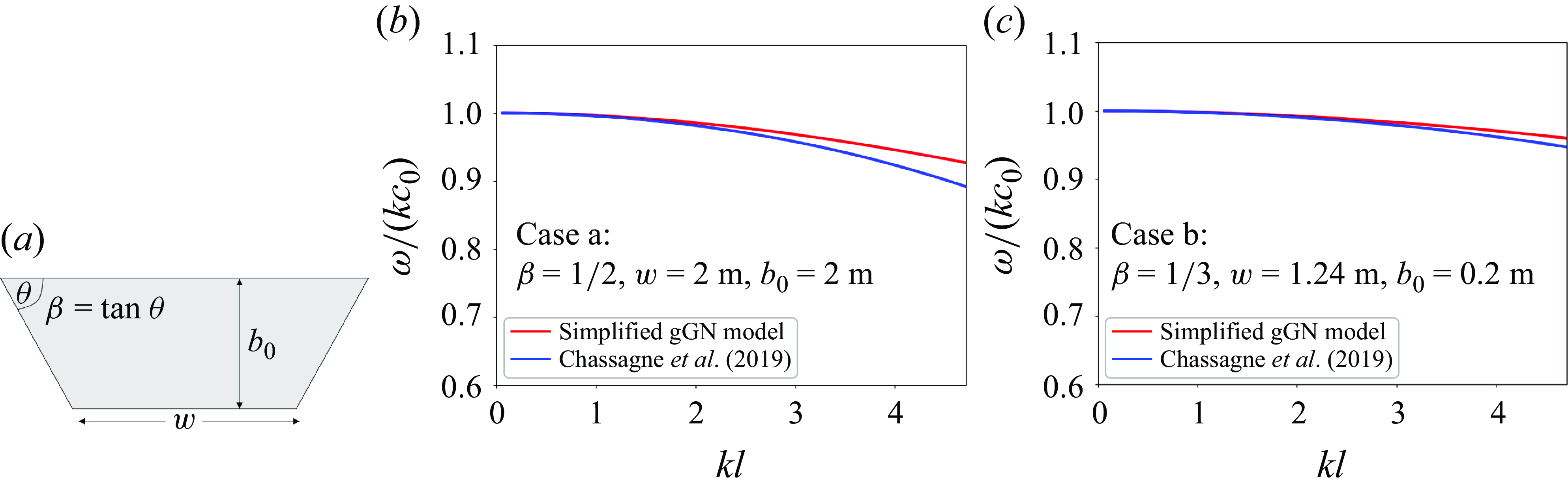
Note that for simple section shapes, as those of figures 1 and 2(a),
 $\overline h_0$
is related to the maximum depth
 $b_0$
by simple geometrical relations (cf. also § 5.4, for explicit formulas in the trapezoidal case).
Using standard techniques, we show that the dispersion relation of the system is
 \begin{equation} \omega ^2 = k^2\dfrac {c_0^2}{ 1 + \frac {\chi }{\overline {h}_0^2} k^2 } \end{equation}
with
 $k$
the wavenumber and
 $c_0=\sqrt {g \bar h_0}$
. In figures 2(b) and 2(c) we show the typical behaviour of the non-dimensional phase speed
 $\omega /kc_0$
as a function of the horizontal reduced wavenumber
 $k{ l}$
, for the case of a trapezoidal section. We consider the case of a deep channel with steep slopes, and of a shallow channel with mild slopes. Using the notation in figure 2(a), these cases correspond, respectively, to
 $(\beta,w,b_0)=(1/2, 2\text{m}, 2\text{m})$
and
 $(\beta,w,b_0)=(1/3,1.24\text{m},0.2\text{m})$
. The latter is representative of the channel used in the well-known experiments by Treske (Reference Treske1994). The coefficient
 $\chi$
is computed from (2.50) with
 ${ l}_2=w$
,
 ${ l}_1={ l}_3=b_0/\beta$
. For completeness, we compare the curves with those obtained using the dispersion relation of the linear model obtained in Chassagne et al. (Reference Chassagne, Filippini, Ricchiuto and Bonneton2019). The curves show comparable trends, with some differences for shorter waves which are within classical modelling error. In particular, for reduced wavenumbers below
 $k { l} = \pi$
the differences observed are within 2 % in the first case, and 0.5 % for the mild slopes.
Dispersion relation for trapezoidal sections: (a) notation, (b) phase speed for a deep channel with steep slopes, (c) shallow channel with mild slopes. Simplified gGN model in blue; linear model of Chassagne et al. (Reference Chassagne, Filippini, Ricchiuto and Bonneton2019) in red.

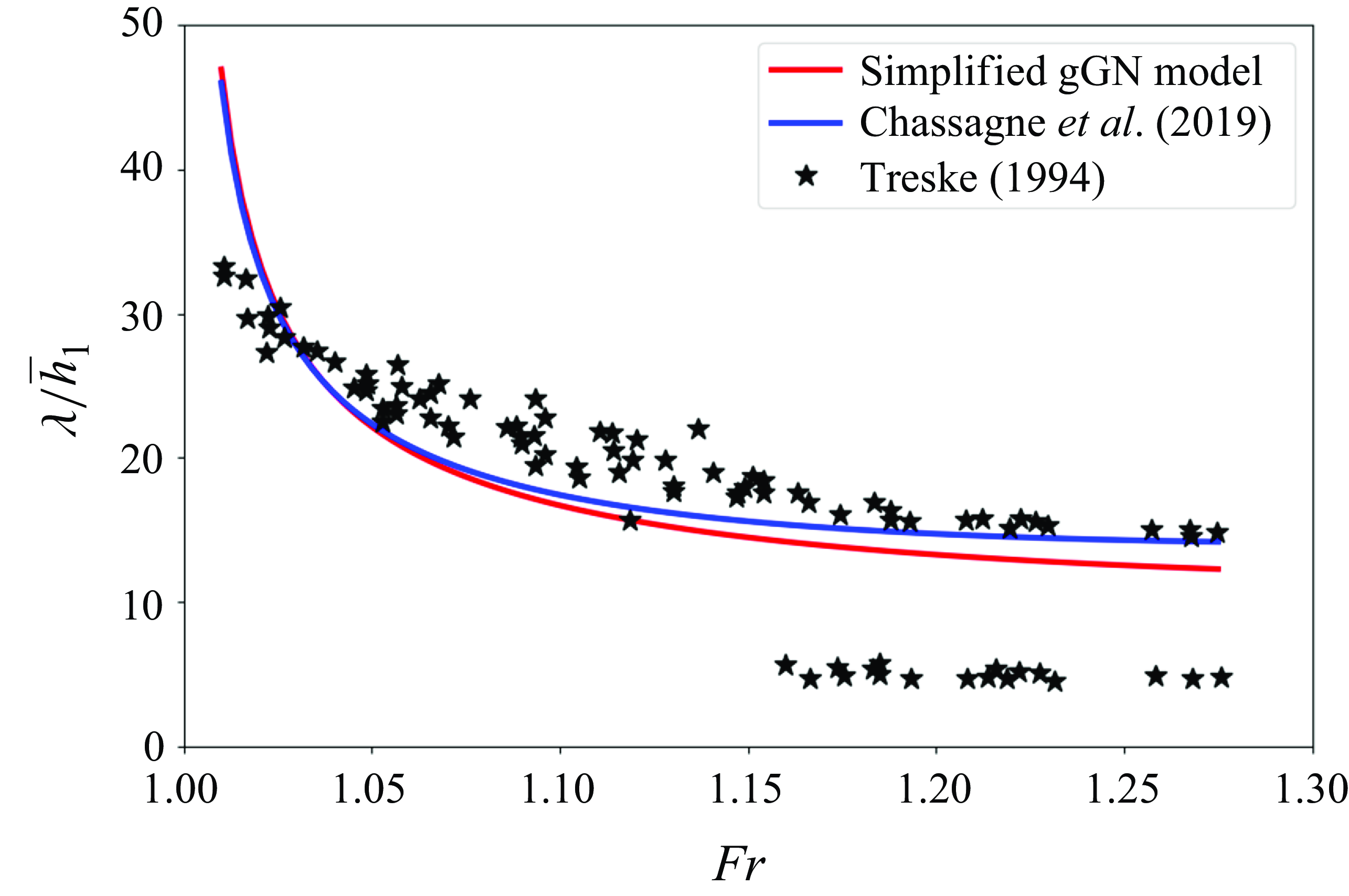
For the second case, representative of the experiments by Treske (Reference Treske1994), we can use the dispersion relation to predict the wavelength-Froude-number dependence. This is achieved by equating the phase velocity to the relative bore speed obtained from the Rankine–Hugoniot relations of the non-dispersive equations. In particular, one looks at the dependence of the wavelength on the relative Froude number defined as
 \begin{equation} \textsf{Fr}:= \dfrac {|\langle u\rangle _2 - c_b|}{\sqrt {g\overline h_1}} \end{equation}
where the subscripts ‘1’ and ‘2’ denote the states ahead of and behind the bore front, whose velocity is denoted by
 $c_b$
. We refer to Lemoine (Reference Lemoine1948), Chassagne et al. (Reference Chassagne, Filippini, Ricchiuto and Bonneton2019) for details. The wavelengths (scaled by
 $\overline h_1$
) predicted theoretically using this method are reported in figure 3. For completeness we also report in the figure the data by Treske (Reference Treske1994), which include both those associated with geometrical dispersion (longer waves), and those measured on the channel axis for high Froude, related to classical non-hydrostatic dispersive effects. Figure 3 shows that the new model provides a good prediction of the long waves associated with geometrical dispersion. The differences with respect to the linear model of Chassagne et al. (Reference Chassagne, Filippini, Ricchiuto and Bonneton2019) for higher Froude numbers is in line with the fact that the simplified gGN provides slightly larger phase celerities for shorter waves, as seen in figures 2(b) and 2(c). Numerical simulation of these experiments using the fully nonlinear equations is discussed in § 5.4.
Lemoine analogy for the experiments by Treske (Reference Treske1994). Comparison of the theoretical predictions using the dispersion relation of the simplified gGN model (blue), with that of Chassagne et al. (Reference Chassagne, Filippini, Ricchiuto and Bonneton2019) (red), and the data by Treske (Reference Treske1994) (symbols).

3.4. Travelling-wave solutions: solitary waves
We show in this section that the system derived admits exact travelling-wave solutions. We focus here on solitary waves. We consider a solitary wave of amplitude
 $a$
and celerity
 $C$
, travelling on a flat water level
 $\overline {h}_{\infty }$
far ahead and far behind. So, let us set
 $\xi = x-Ct$
and assume that at time
 $t=0$
the peak is at
 $x=0$
. We now seek solutions of the form
 \begin{align} \overline h = \overline h(\xi), \quad \langle u\rangle = \langle u\rangle (\xi). \end{align}
We can readily write from the mass conservation law that
 \begin{align} \overline {h}(\langle u\rangle -C)= m=const, \end{align}
Which, using the conditions at infinity, gives the relations
 \begin{equation} \langle u\rangle = \left(1- \dfrac {\overline {h}_{\infty } }{\bar h}\right) C\;,\quad m=- \overline {h}_{\infty }C \end{equation}
The momentum equation implies
 \begin{equation} \overline {h}(\langle u\rangle -C)^2+\frac {g\overline {h}^2}{2}- \chi \ddot \tau =q=const. \end{equation}
Since
 $\ddot \tau =(\langle u\rangle -C)((\langle u\rangle -C)\tau ^{\prime})^{\prime}=m^2\tau (\tau \tau ^{\prime})^{\prime}$
(here ‘prime’ means the derivative with respect to
 $\xi$
), one obtains
 \begin{equation} m^2 \tau +\frac {g}{2\tau ^2}-\chi m^2\tau (\tau \tau ^{\prime})^{\prime}=q=const. \end{equation}
Let
 $\tau _\infty =1/\overline {h}_\infty$
. Then one can find
 $q$
and we have
 \begin{equation} m^2 (\tau -\tau _\infty)+\frac {g}{2}\left (\frac {1}{\tau ^2}-\frac {1}{\tau _\infty ^2}\right)-\chi m^2\tau (\tau \tau ^{\prime})^{\prime}=0. \end{equation}
Multiplying by
 $\tau ^{\prime}$
, one can integrate it again:
 \begin{align} m^2 (\tau -\tau _\infty)^2+g\left (-\frac {1}{\tau }+\frac {1}{\tau _\infty }-\frac {\tau }{\tau _\infty ^2}+\frac {1}{\tau _\infty }\right)-\chi m^2(\tau \tau ^{\prime})^2=0. \end{align}
We rewrite this equation as
 \begin{equation} \chi m^2\tau ^2 \tau ^{\prime2}=F(\tau),\quad F(\tau)= m^2(\tau -\tau _{\infty })^2-\frac {g}{\tau \tau _{\infty }^2}(\tau -\tau _{\infty })^2. \end{equation}
On can remark that at
 $\tau =\tau _\infty$
, one has
 $F=0$
,
 $F^{\prime}=0$
. Moreover,
 $F^{\prime\prime}\gt 0$
if
 $m^2\gt g/\tau _\infty ^3$
. If the velocity
 $\langle u\rangle _\infty =0$
, the last inequality means that the Froude number should be larger than one (a classical inequality for the existence of solitary waves). Since
 $F\rightarrow -\infty$
as
 $\tau \rightarrow 0$
, it implies that there exists
 $\tau _0 \lt \tau _\infty$
such that
 $F(\tau _0)=0$
. It implies the existence of supercritical solitary waves having the amplitude
 $a= \overline h_0-\overline h_\infty, \; \overline h_0=1/\tau _0.$
We can now evaluate the earlier relation at the peak; where
 $\tau ^{\prime}=0$
we have
 $\tau _0 =1/\overline {h}_0= 1/(\overline {h}_\infty +a)$
. We thus obtain a relation celerity/amplitude:
 \begin{align} 0=m^2 \dfrac { a^2 }{\overline {h}_\infty ^2(\overline {h}_\infty +a)^2} - \dfrac {g a^2}{\overline {h}_\infty +a}. \end{align}
Using the constancy of
 $m$
, we can also deduce
 $m^2 = C^2\overline h_{\infty }^2$
which allows the compatibility relations to be derived:
 \begin{equation} C^2 = g(\overline {h}_\infty +a) = g\overline {h}_0=\dfrac {g}{\tau _0}\;,\quad m^2 = g(\overline {h}_\infty +a)\overline {h}_\infty ^2=\dfrac {g}{\tau _0\tau _{\infty }^2}. \end{equation}
Combining all of these results, we end with the nonlinear ordinary differential equation (ODE)
 \begin{equation} \tau ^{\prime 2} = \dfrac {(\tau -\tau _\infty)^2(\tau -\tau _0)}{\chi \tau ^3}. \end{equation}
The simplest way to solve it is to only construct a half-width solitary wave with initial condition
 $\tau =\tau _0$
at
 $\xi =0$
.
In practice, we have actually solved (3.20) using the basic odeintmethod in numpy, starting from the peak with given zero derivative, and the known value of
 $\tau =\tau _0$
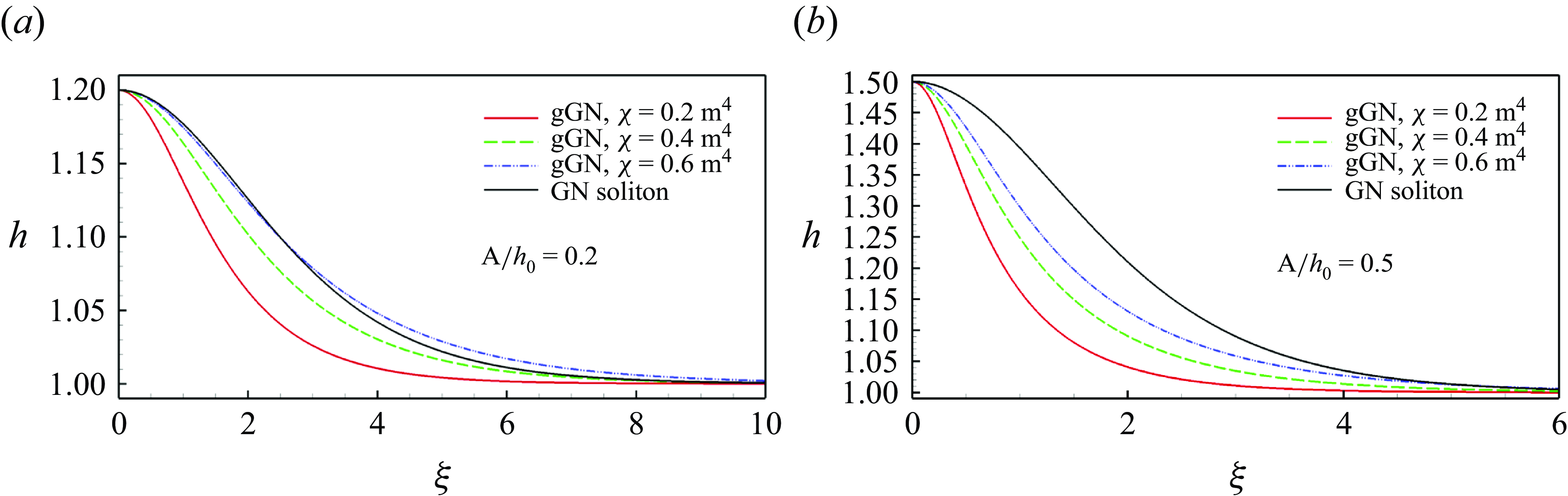
. Typical shapes of the solitary waves obtained for two different values of the nonlinearity
 $\epsilon =a\tau _{\infty }$
, and of the dispersion parameter
 $\chi$
are reported in figure 4. For the sake of comparison, we report the SGN solitary wave with the same amplitude. The solitary wave of the new system generally has a more ‘peaky’ shape, and a strong dependence on the relative values of
 $\chi$
and
 $\epsilon$
.
Solitary waves obtained for values of
 $\chi \in \{0.2,\,0.4,\,0.6\}\text{m}^4$
, and nonlinearity
 $ \epsilon =0.2$
(a) and
 $ \epsilon =0.5$
(b).

3.5. Travelling waves solutions: a composite solution
Equation (3.19) allows solutions of other forms than solitary waves, including e.g. periodic solutions, to be obtained. Following the approach by Gavrilyuk et al. (Reference Gavrilyuk, Nkonga, Shyue and Truskinovsky2020), we exploit this property to show the existence of exact composite travelling waves involving two moving profiles connected via a generalised Rankine–Hugoniot relation. Equation (3.19) multiplied by
 $\tau ^{\prime}$
can be integrated in a more general form as
 \begin{equation} \chi \tau ^3(\tau ^{\prime})^2= (\tau -\tau _1)(\tau -\tau _2)(\tau -\tau _3), \quad 0\lt \tau _1\lt \tau _2\lt \tau _3. \end{equation}
This equation describes a periodic wave oscillating between the depths
 $\bar h_1=1/\tau _1$
and
 $\bar h_2=1/\tau _2$
. The third root
 $\tau _3$
controls the wave shape. If
 $\tau _3=\tau _2=\tau _\infty$
, one obtains (3.25) and goes back to a single solitary wave. One can show that the three roots verify the constraint (see Gavrilyuk et al. (Reference Gavrilyuk, Nkonga, Shyue and Truskinovsky2020) for details)
 \begin{equation} m^2\tau _1\tau _2\tau _3=g. \end{equation}
To construct a stable solution, we follow a procedure similar to that used in Gavrilyuk et al. (Reference Gavrilyuk, Nkonga, Shyue and Truskinovsky2020) for the Serre–Green–Naghdi equations.
-
(i) Choose three roots such that
$0\lt \tau _1 \lt \tau _2\lt \tau _3$
, with
$\tau _2$
and
$\tau _3$
close to each other. -
(ii) Choose a sign for the mass flow obtained from (3.27). For
$m\lt 0$
, we obtain a right travelling wave. -
(iii) Give an arbitrary value to the velocity corresponding to the state
$\tau _2$
. For example,
$u_2=0$
. Compute the celerity
$C$
of the periodic travelling wave from
,
$\bar h_2=1/\tau _2$
. Thus, the periodic travelling wave is perfectly defined. -
(iv) From (3.26), we obtain the value of the second derivative
$\tau ^{\prime\prime}\vert _{\tau =\tau _1}$
:(3.28)
\begin{equation} 2\chi \tau _1^3\tau ^{\prime\prime}\vert _{\tau =\tau _1} =(\tau _1-\tau _2)(\tau _1-\tau _3)\gt 0. \end{equation}
-
(v) Compute the values
$(h_{\star }, u_{\star })$
which satisfy the generalised Rankine–Hugoniot relations (including dispersive terms):(3.29)(3.30)
\begin{equation} m^2 \tau _1+\frac {g}{2\tau _1^2}-\chi m^2\tau _1^2 \tau ^{\prime\prime}\vert _{\tau =\tau _1} =m^2 \tau _\star +\frac {g}{2\tau _\star ^2}, \end{equation}
with as usual
$\tau _\star =1/h_\star$
. As shown in Gavrilyuk et al. (Reference Gavrilyuk, Nkonga, Shyue and Truskinovsky2020), if we choose the root
$\tau _\star$
closest to
$\tau _2$
, then the solution having the constant state
$\star$
on the left and the corresponding periodic travelling wave on the right, is stable. -
(vi) Introduce a regularisation of the jump using, for example, a half-width solitary wave from
$h_\star =1/\tau _\star$
to
$h_1=1/\tau _1$
(in
$h$
variables).


To build this solution in practice, given as data the tuple
 $(\tau _1,\tau _2,\tau _3)$
, we first solve for
 $\tau _\star$
, and then integrate (3.26) with initial value
 $\tau _1$
to compute the periodic branch. The integration is done in practice recasting (3.26) as
 \begin{equation} \begin{aligned} 2\chi \left(\tau \tau ^{\prime}\right)^{\prime} = &\left( 1 -\dfrac {\tau _2}{\tau }\right)\left( 1-\dfrac {\tau _3}{\tau }\right) +\left( 1-\dfrac {\tau _1 }{\tau }\right)\left( 1-\dfrac {\tau _3}{\tau }\right) \\ &+ \left( 1-\dfrac {\tau _1}{\tau }\right)\left( 1-\dfrac {\tau _2}{\tau }\right) - \left(1-\dfrac {\tau _1}{\tau }\right)\left( 1-\dfrac {\tau _2}{\tau }\right)\left( 1-\dfrac {\tau _3}{\tau }\right), \end{aligned} \end{equation}
which is integrated with initial conditions
 $(\tau, \tau ^{\prime}) = (\tau _1, 0)$
. The results presented have been obtained using the 8th order Runge–Kutta method in the SciPyclass solve_ivp, with relative and absolute tolerances rtol =
 $10^{-8}$
and atol =
 $10^{-12}$
. Concerning the regularisation, we have computed the half solitary wave as discussed in the previous section.
As an example, let us take
 $(\tau _1, \tau _2, \tau _3)=(1 \text{m}^{-1}, 1.3\text{m}^{-1}, 1.301\text{m}^{-1}$
) and
 $\chi =0.4$
m
 $^4$
. For this choice, we obtain
 $\tau _{\star} =1.300\,500\,319\,855\,95$
m
 $^{-1}$
 $\lt \tau _1$
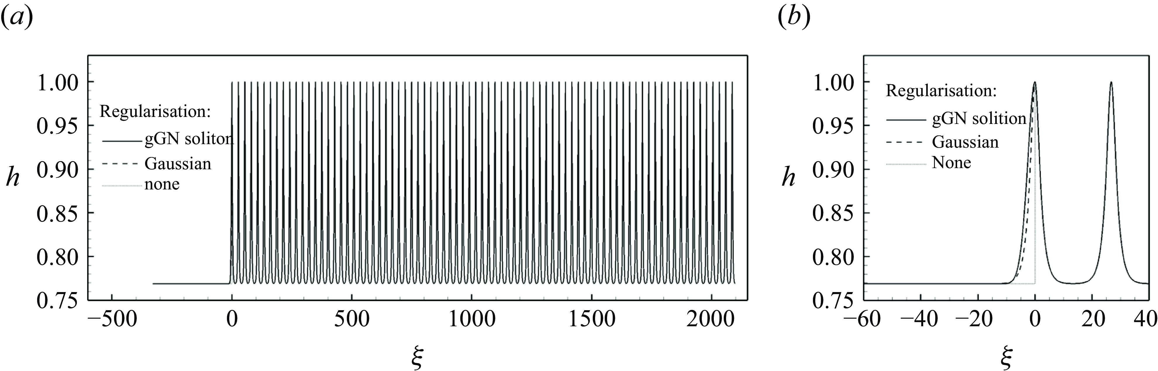
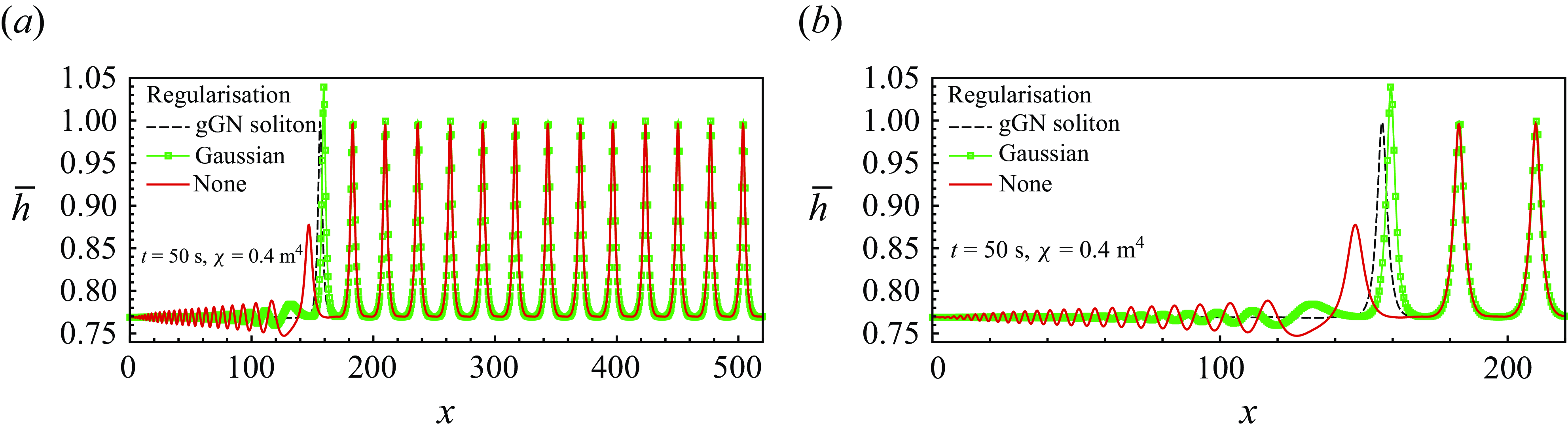
. Integrating the ODEs, we obtain the solution plotted in figure 5. In the figure, we also compare three treatments of the transition: that obtained using a gGN solitary wave, a Gaussian
 $\textrm e^{-(x/L)^2}$
with
 $L=8$
m, and no regularisation. We will compare the evolution of the three later in the results section.
Composite travelling wave solution obtained for
 $\chi =0.4$
m
 $^4$
, setting
 $\tau _1=1$
m
 $^{-1}$
,
 $\tau _2=1.3$
m
 $^{-1}$
and
 $\tau _3=1.301$
 $\text{m}^{-1}$
. (a) Solution on the whole domain [–350, 2100] m. (b) Zoom of the regularised jump and first peak.

4. System reformulations and numerical approximation
Using well-established numerical methods, numerical tests are performed for two different reformulations of the dispersive model. This section describes in some detail the form of the equations used for the discretisation, recalling their main properties. The description of the numerics is left for completeness in Appendix C.
For simplicity, and unless otherwise specified, in the remainder of the paper we will use the notation
 $h$
and
 $u$
for the average depth and Favre-averaged velocity.
4.1. Elliptic–hyperbolic approximation
We first consider a splitting of the original system in an elliptic and a hyperbolic step. This is a rather classical idea used in many works (Wei et al. Reference Wei, Kirby, Grilli and Subramanya1995; Le Métayer et al. Reference Le Métayer, Gavrilyuk and Hank2010; Bonneton et al. Reference Bonneton, Chazel, Lannes, Marche and Tissier2011; Parisot Reference Parisot2019; Gavrilyuk & Shyue Reference Gavrilyuk and Shyue2024).
More specifically, here we follow the reformulation introduced in Filippini et al. (Reference Filippini, Kazolea and Ricchiuto2016) and Kazolea, Filippini & Ricchiuto (Reference Kazolea, Filippini and Ricchiuto2023) for the Serre–Green–Naghdi equations, and applied to other Boussinesq models in Cauquis, Ricchiuto & Heinrich (Reference Cauquis, Ricchiuto and Heinrich2022), Torlo & Ricchiuto (Reference Torlo and Ricchiuto2023), Jouy et al. (Reference Jouy, Violeau, Ricchiuto and Le2024). The idea is to write the system as a perturbation to the shallow-water equations via an algebraic source. The compatibility with the original equations leads to an elliptic problem for the latter. To obtain this form, we start by using the relation
 \begin{equation} \begin{aligned} h^2\ddot \tau = h ( u_x)^2 + h( u_{xt} + u u_{xx}) = h ( u_x)^2 + h\dot u_x = h( u_t + u u_x)_x = h ( \dot u)_x \end{aligned}, \end{equation}
where
 \begin{align} \dot u_x = ( u_{xt} + u u_{xx}) \ne (\dot u)_x=( u_t + u u_x)_x. \end{align}
Using this, equation (2.47) can be recast as
 \begin{equation} (hu)_t +\left(hu^2+ g\frac {h^2}{2}\right)_x = \left[ \dfrac {\chi }{ h} (\dot u)_x\right]_x. \end{equation}
Now following Filippini et al. (Reference Filippini, Kazolea and Ricchiuto2016), we introduce the variable
 $\phi$
satisfying
 \begin{equation} h \phi:= (hu)_t + (hu^2 + g h ^2/2)_x \Rightarrow \phi - gh_x= \dot u. \end{equation}
We can now combine this definition with the compatibility requirement
 \begin{align} h\phi = \left[ \dfrac {\chi }{ h} (\dot u)_x \right]_x \end{align}
and obtain the equation for
 $\phi$
:
 \begin{align} \begin{aligned} h\phi =\left[ \dfrac {\chi }{ h} ( \phi - gh_x)_x \right]_x. \end{aligned} \end{align}
The dispersive system (2.46), (2.47), (2.48) can thus be recast as
 \begin{equation} \begin{aligned} h \phi - \chi \left[\dfrac {1}{ h}( \phi - g h_x)_x\right]_x &= 0\\ h_t + ( h u)_x &= 0\\ (hu)_t + (hu^2 + g h^2/2)_x &= h \phi, \end{aligned} \end{equation}
which gives two operators. The first an elliptic problem for the auxiliary variable
 $\phi$
, whose variational form reads
 \begin{equation} \int v h \phi +\chi \int v_x \tau \phi _x= \chi \int v_x\tau \delta _x, \end{equation}
where
 $v$
is a test function with compact support
 $v \in H^1_0$
, and having set
 $\delta:= gh_x$
. We can have the following simple characterisation.
Proposition 3 (Coercivity of the elliptic operator). Provided there exist solution-independent uniformly bounded values
 $h_{min }\gt 0$
, and
 $h_{max }\lt \infty$
such that
 $h\in (h_{min },h_{max })$
, then the variational form (4.8) is uniformly coercive.
Proof.
Under the hypotheses made, we can easily show the
 $H^1$
norm equivalence
 \begin{align} \dfrac {\chi C_{min }}{h_{max }} \|\phi \|_{H^1}^2 \leqslant \int h \phi ^2 +\chi \int \tau (\phi _x)^2 \leqslant \dfrac {\chi C_{max }}{h_{min }} \|\phi \|_{H^1}^2 \end{align}
for any
 $C_{\textit{max}} \ge \max \bigg( 1 ,\dfrac{h_{\textit{min}}h_{\textit{max}}}{\chi} \bigg)$
and
 $C_{\textit{max}} \le \min \bigg( 1 ,\dfrac{h_{\textit{min}}h_{\textit{max}}}{\chi} \bigg)$
The last two equations in (4.7) define a hyperbolic evolution operator for the shallow-water variables, with an extra algebraic forcing term linear in
 $\phi$
.
The system can be effectively integrated in time and space. Here the elliptic step is discretised using a standard finite element method. The hyperbolic part is evolved with an explicit two-stage residual distribution scheme. Details are given in Appendix C.
4.2. Hyperbolic relaxation
To avoid the inversion of an elliptic operator, we replace the original system by an approximate hyperbolic system which can be treated numerically with classical techniques also used for the Saint–Venant equations (Mazaheri, Ricchiuto & Nishikawa Reference Mazaheri, Ricchiuto and Nishikawa2016; Favrie & Gavrilyuk Reference Favrie and Gavrilyuk2017; Busto et al. Reference Busto, Dumbser, Escalante, Favrie and Gavrilyuk2021). Because of the variational formulation discussed in § 3.2, we will use the method of augmented Lagrangian proposed in Favrie & Gavrilyuk (Reference Favrie and Gavrilyuk2017), Dhaouadi, Favrie & Gavrilyuk (Reference Dhaouadi, Favrie and Gavrilyuk2019). Compared with other approaches, this technique preserves the variational structure of the equations, thus guaranteeing the existence of an exact energy conservation law also for the approximate system. A rigorous asymptotic analysis and justification of this approach is given in Duchêne (Reference Duchêne2019).
In this method, we introduce an auxiliary variable
 $\eta (t,x)$
satisfying the second-order equation
 \begin{equation} \ddot \eta +\frac {\mu }{\chi } \left (\eta -\tau \right)=0. \end{equation}
This equation can be written as a first-order quasilinear system:
 \begin{align} \eta _t + u \eta _x = w, \end{align}
 \begin{align} w_t + uw_x = -\frac {\mu }{\chi } \left ( \eta - \tau \right). \end{align}
To couple the evolution of
 $\eta$
to the other quantities, we consider the augmented system
 \begin{equation} \begin{aligned} h_t +&(hu)_x =0, \\ (hu)_t +&(hu^2+ p_{tot})_x=0,\\ \left ( h \eta \right)_t +&\left (hu \eta \right)_x =h w,\\ \left (hw \right)_t +&\left (hu w \right)_x = -\frac {\mu }{\chi } \left (h \eta - 1\right). \end{aligned} \end{equation}
with the closure relation
 \begin{equation} p_{tot}= g\frac {h^2}{2} + \mu \tau \left ( h \eta -1\right)= g\frac {h^2}{2} + \mu \left ( \eta -\tau \right). \end{equation}
As shown in Duchêne (Reference Duchêne2019),
 $\eta$
is an order
 $\mathcal{O}(\mu)$
asymptotic approximation of
 $\displaystyle \tau (t,x)=1/ h(t,x)$
. So
 $\mu$
is a large positive parameter, which allows
 $\eta$
to relax to
 $\displaystyle \tau (t,x)$
. In the limit
 $\mu \rightarrow \infty$
, we recover the original system, and, in particular, the total pressure
 $p_{tot}$
becomes
 \begin{equation} p_{tot}=\frac {gh^2}{2}-\chi \ddot {\tau }. \end{equation}
The system is hyperbolic with eigenvalues
 \begin{equation} \lambda _1=u-c, \quad \lambda _{2, 3 }=u, \quad \lambda _4=u+c, \end{equation}
having set
 \begin{equation} c^2=gh+ \mu \tau ^2. \end{equation}
Following Dhaouadi et al. (Reference Dhaouadi, Favrie and Gavrilyuk2019) and Tkachenko et al. (Reference Tkachenko, Gavrilyuk and Massoni2023), one can show that (4.13) are the Euler–Lagrange equations for the Lagrangian:
 \begin{align} L=\int _{-\infty }^{+\infty }\left (h\frac {u^2}{2}-W(h, \eta, \dot {\eta })\right)\text{d}x, \end{align}
with
 \begin{align} W(h, \eta, \dot {\eta })=\frac {gh^2}{2}-\frac {\chi \, h\, \dot {\eta }^2}{2}+\frac {\mu \, h}{2} \left (\eta -\frac {1}{h}\right)^2. \end{align}
The pressure
 $p_{tot}$
is defined as the partial Legendre transform with respect to
 $h$
 \begin{equation} p_{tot}=h\frac {\partial W}{\partial h}-W=\frac {gh^2}{2}+\mu \left (\eta -\tau \right), \end{equation}
and (4.10) is equivalent to the Euler–Lagrange equation for
 $\eta$
 \begin{equation} \frac {\partial W}{\partial \eta }-\frac {\partial }{\partial t}\left (\frac {\partial W}{\partial \dot \eta }\right)-\frac {\partial }{\partial x}\left (\frac {\partial W}{\partial \dot \eta }u\right)=0. \end{equation}
To integrate these hyperbolic equations numerically, we use an explicit two-stage residual distribution scheme, coupled to a Strang splitting in time to treat the stiff source term. Details are given in Appendix C.
5. Numerical tests
5.1. Verification using analytical solutions
5.1.1. Solitary waves
We have performed a verification of the 1-D solver using the solitary wave solution of § 3. We discuss here the case of a solitary wave of nonlinearity
 $\epsilon =a\tau _{\infty }=0.2$
, and we consider the case
 $\chi =0.4$
(cf. figure 4
a) and
 $h_{\infty }=1$
m. The behaviour with other values of the parameters is very similar.
We have considered a solitary wave whose peak is positioned initially at
 $x_0 = -100$
m in the the spatial domain
 $[-200, 200]$
m. The soliton propagation over a distance
 $L=200$
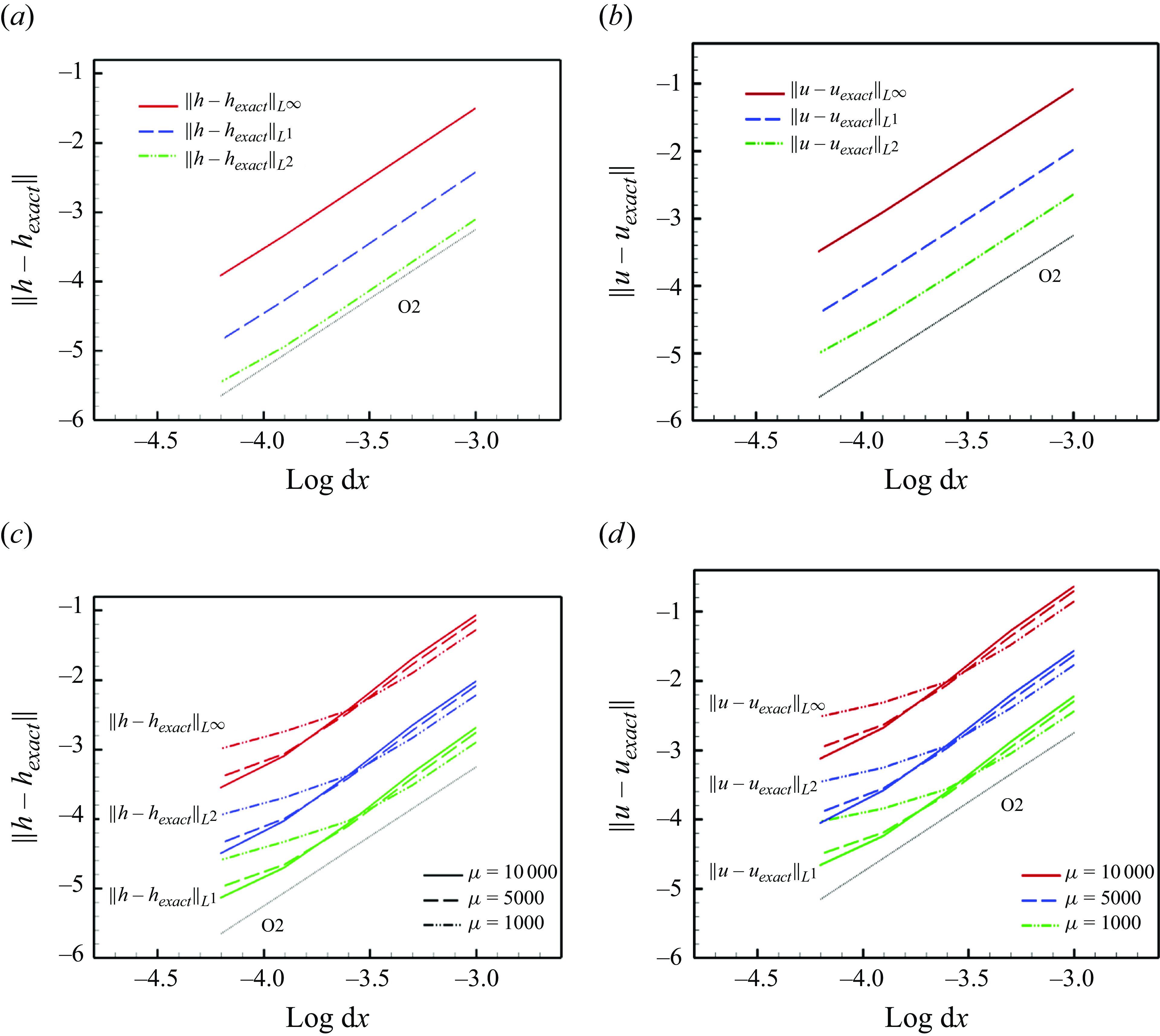
m has been computed on several mesh resolutions using both the elliptic–hyperbolic formulation, and the hyperbolic relaxation form. We report in figure 6 the resulting grid convergence of the errors, defined as the difference between the computed and exact depth, and velocity. Figures 6(a) and 6(c) show that with the elliptic–hyperbolic formulation we can achieve the expected second order of convergence in all the norms, for both depth and velocity.
For the hyperbolic reformulation, figures 6(b) and 6(d) show a dependence of the convergence rates on the value of the relaxation constant
 $\mu$
. Already for
 $\mu =1000$
the error convergence rates reduce on finer meshes. This is due essentially to the modelling error for finite
 $\mu$
. Values of
 $\mu$
of order
 $10^4$
are necessary to correct this. However, such values negatively affect the computational time, due to the time-step restriction (cf. equation (C19) in Appendix C).
Grid convergence to a solitary wave with nonlinearity
 $\epsilon =0.2$
and
 $\chi =0.4m^4$
. (a) Depth error for the elliptic–hyperbolic formulation. (b) Depth error for the hyperbolic formulation for different
 $\mu$
. (c) Velocity error for the elliptic–hyperbolic formulation. (d) Velocity error for the hyperbolic formulation for different
 $\mu$
. With standard notations,
 $L^1$
,
 $L^2$
and
 $L^\infty$
are used for the norms in the corresponding functional spaces. The sub-script ‘exact’ denotes the values corresponding to the exact solitary waves. With
 $\textrm{O}2$
is the theoretical slope for second order of accuracy.

To clarify the impact of this on the qualitative behaviour of the model, we have looked at the convergence of the solution with
 $\mu$
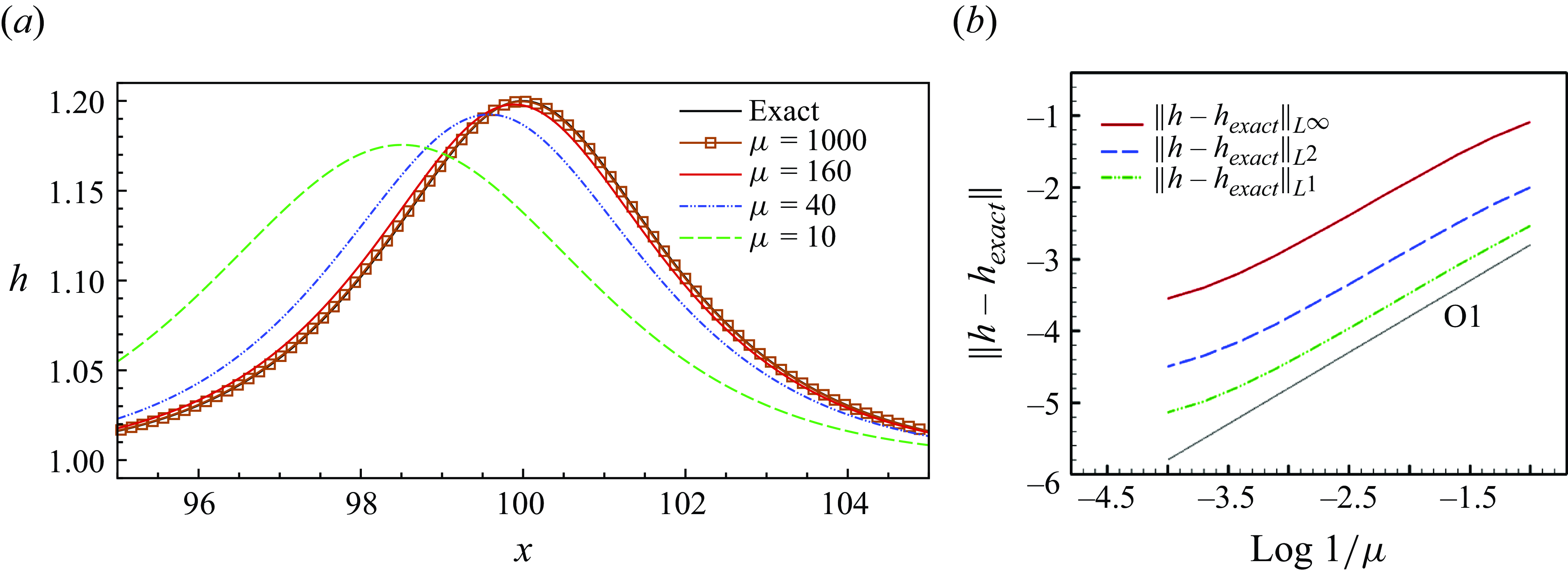
. The results are summarised in figure 7. In particular, figure 7(a) shows the wave profile of the solitary wave obtained numerically at final time. Despite what the error convergence suggests, clearly there is no visual difference in the solutions when using values of
 $\mu$
above
 $\, 10^3$
. This is reassuring concerning the use of the hyperbolic approximation in physical applications, although the specific optimal value of
 $\mu$
may depend on the problem parameters. Figure 7(b) depicts the convergence of the depth with respect to
 $\mu$
, showing the expected first-order rate.
Convergence to a solitary wave with nonlinearity
 $\epsilon =0.2$
and
 $\chi =0.4$
m
 $^4$
. (a) Depth distribution at final time obtained with the hyperbolic reformulation and different
 $\mu$
. (b) Depth error convergence with
 $\mu$
. With
 $\textrm{O}1$
is the theoretical first order slope.

5.1.2. Composite solution
We now consider computations of the composite travelling-wave solution of § 3.4. Besides further verifying the implementation, the numerical study tries to clarify the role of the regularisation. As a first exercise, we perform a grid convergence study. We start from the initial solution with values provided at the end of § 3.4 (cf. figure 5), using the regularisation with half-width gGN solitary wave. Simulations are run on the computational domain
 $[-100, 2300]$
m, with the initial jump at the origin. Free boundary conditions are imposed on the right, while the constant solution is imposed on the left. We let the model evolve the flow for
 $50$
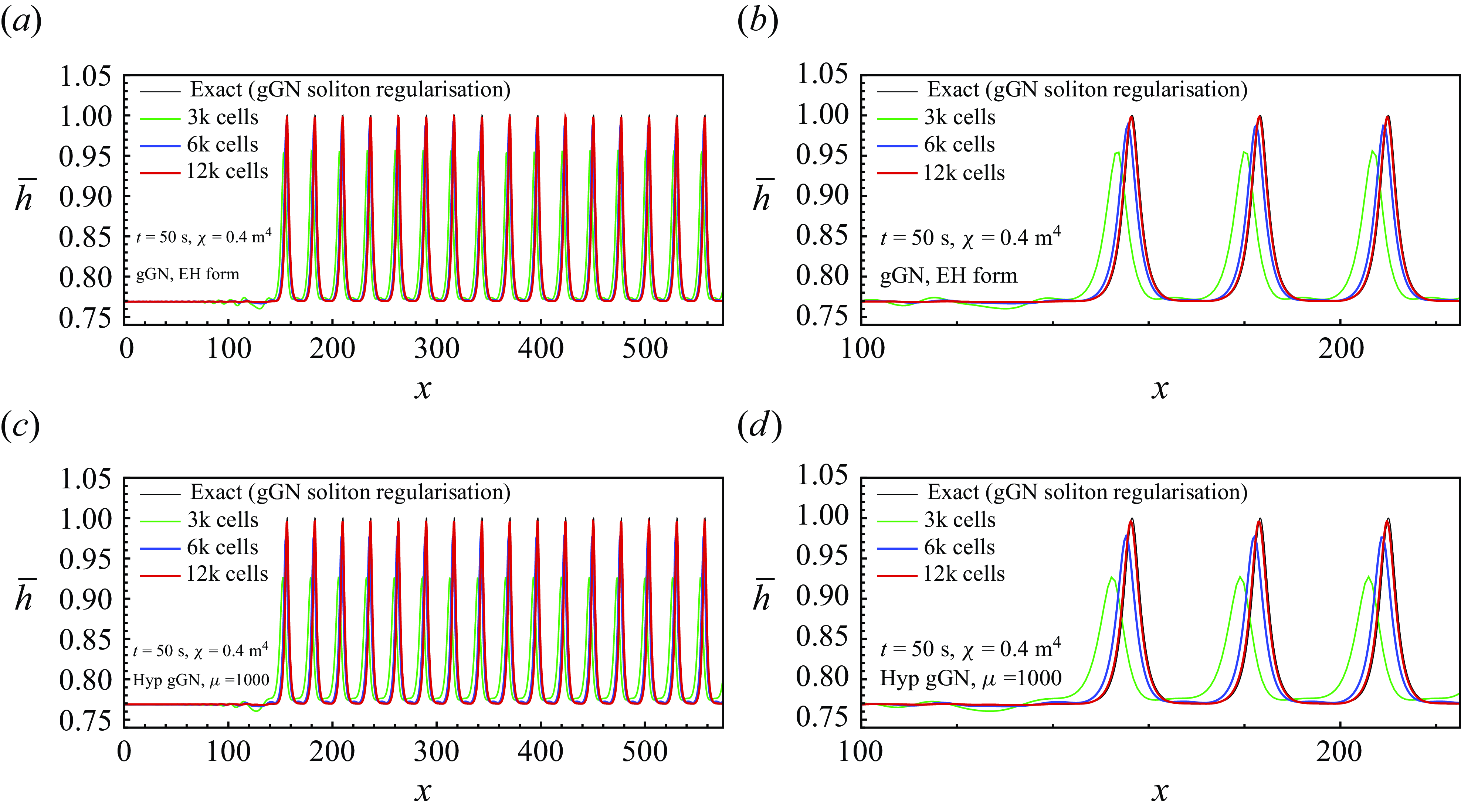
s, and then compare with the initial solution translated by the exact celerity computed analytically. The results are reported in figure 8.
Grid convergence toward the regularised composite solution of § 3.5. (a) Depth at
 $t=50$
s obtained with the elliptic–hyperbolic approximation. (b) Close-up view of the first peaks obtained with the elliptic–hyperbolic approximation. (b) Depth at
 $t=50$
s obtained with the hyperbolic formulation with
 $\mu =1000$
. (d) Close-up view of the first peaks obtained with the hyperbolic formulation.

To give a more general view, we report in figure 8 both the solutions in the subdomain
 $[0,575]$
m, and zoom of the first peaks, including the regularised one. As one can see, both numerical approximations of the model converge nicely to the travelling solution. Quite interestingly, the results converge to the translated initial solution, including the regularisation. This suggests that the actual solution admitted is composed from a constant state, obtained from the Rankine–Hugoniot relations, and an infinite series of oscillations between the values
 $\tau _1$
and
 $\tau _2$
, much resembling an infinite series of solitary waves propagating at the level
 $\tau _2$
.
Composite solution: influence of the regularisation of the initial solution.

To get more insight into this, we have performed the same simulation with the different regularisation strategies discussed in § 3.4. Grid-converged results are reported in figure 9. Clearly, past the regularised peak, the three cases provide an identical infinite train of waves. Secondly, the initialisation with a half-width solitary wave is the only case which does not introduce any secondary waves, to which the numerical approximation converges as the mesh is refined. This indicates that the exact solution is not a discontinuous one in a classical sense, but rather a composite solution composed of a constant state
 $\star$
, and a periodic wave train of waves of large length. This travelling-wave solution verifies the generalised Rankine–Hugoniot conditions coming from the mass and momentum equations. In this sense, it is a ‘discontinuous’ solution of the gGN equations. Such solutions are related to shock solutions of the corresponding Whitham system (see e.g. Gavrilyuk & Shyue (Reference Gavrilyuk and Shyue2021) for the study of the Benjamin–Bona–Mahony equation).
5.2. Breakdown of a Gaussian water column
We pass now to the study of the behaviour of the model. To begin with, we consider a simple case consisting of the breakdown of a Gaussian water column for which the initial state is given by
 \begin{align} h(x,t=0) = h_{\infty }\left( 1 + \epsilon \textrm e^{- (x-x_0)^2/L^2}\right)\;,\quad u(x,t=0) =0. \end{align}
We start by investigating the propagation properties of the simplified gGN model with respect to the dispersion and nonlinearity parameters
 $\chi$
and
 $\epsilon$
. To this end, we consider six cases corresponding to two values
 $\chi =0.1$
m
 $^4$
and
 $\chi =0.6$
m
 $^4$
, and three nonlinearity values:
 $\epsilon =0.125$
,
 $\epsilon =0.25$
and
 $\epsilon =0.5$
. We consider a computational domain
 $[-150,150]$
m, on which we set the initial Gaussian centred in
 $x_0=0$
, and we take
 $L=2$
m and
 $h_{\infty }=2$
m as well. We simulate with both solution methods the evolution of the initial column up to time
 $16$
s using
 $N=10^4$
cells, and taking a value
 $\mu =10^{3}$
in the hyperbolic relaxation formulation.
Breakdown of a Gaussian water column: solutions at time
 $t=16$
s. Plots with (a)
 $\epsilon = 0.125$
,
 $\chi =0.1\text{m}^4$
; (b)
 $\epsilon = 0.125$
,
 $\chi =0.6\text{m}^4$
; (c)
 $\epsilon = 0.25$
,
 $\chi =0.1\text{m}^4$
; (d)
 $\epsilon = 0.25$
,
 $\chi =0.6\text{m}^4$
; (e)
 $\epsilon = 0.5$
,
 $\chi =0.1\text{m}^4$
; (f)
 $\epsilon = 0.5$
,
 $\chi =0.6\text{m}^4$
. Solid line, elliptic–hyperbolic system;
 , hyperbolised system with
 $\mu =1000$
.

The results are visualised in figure 10. Several remarks can be made. First of all, the two different formulations provide almost identical results, which is a further verification (albeit indirect) of our implementation. Furthermore, comparing the left and right columns, we can see that higher values of
 $\chi$
result in longer waves, as one may expect since in this case the dispersive regularisation has more weight. The lower value of
 $\chi$
results in shorter and taller waves, with stronger and more localised oscillations. These differences are enhanced when considering increasing values of nonlinearity. Note that as the discussion of § 2.4 shows, for a given section shape, higher values of
 $\chi$
may correspond either to deeper channels or to larger ones.
5.2.1. Validation against section averaged 2-D shallow-water simulations
Since for this case there is no exact solution, we consider a validation against section averaged full 2-D shallow-water computations. The latter have been run with the solver developed in the series of works Ricchiuto (Reference Ricchiuto2015), Arpaia & Ricchiuto (Reference Arpaia and Ricchiuto2018, Reference Arpaia and Ricchiuto2020), and thoroughly validated on a wide range of cases against analytical and experimental data.
The set-up of the 2-D simulations is the following. We consider three sections: symmetric trapezoidal; symmetric triangular; non-symmetric trapezium. Note that the last is out with the hypotheses of the model. It is included in the study for the sake of generality, and to test the limit of our derivation. Following the notation of figures 1(b) and 1(c) in § 2, we fix the value of
 $b_0$
, and then choose appropriate values of the remaining lengths for each section type to obtain the correct value of
 $\chi$
. For the case
 $\chi =0.1$
m
 $^4$
, we set
 $b_0 =2.5$
m. We then choose
 $({ l}_1, { l}_2, { l}_3) = (1.07, 0.36,1.07)$
m in the symmetric trapezoidal case, and
 $({ l}_1, { l}_2, { l}_3) = (1.385\,75, 0.0,1.385\,75)$
m in the triangular one. For the non-symmetric trapezium, we choose
 $({ l}_1, { l}_2, { l}_3) = (1.284, 0.36,0.7249)$
m. For
 $\chi =0.6$
m
 $^4$
, we have set
 $b_0 =2.75$
m, and chosen
 $({ l}_1, { l}_2, { l}_3) = (2.165, 1.1175,2.165)$
m in the trapezoidal case, and
 $({ l}_1, { l}_2, { l}_3) = (3.0855, 0.0,3.0855)$
m in the triangular one. Also in this case, we have computed solutions with a non-symmetric trapezoidal section obtained with
 $({ l}_1, { l}_2, { l}_3) = (2.598, 1.1175,1.146\,68)$
m.
In all cases, the initial solution is then set using (2.9):
 \begin{align} h(x,y,t=0) = \overline {h}(x,t=0) - b(y) + \overline {b} = h_{\infty }( 1 + \epsilon \textrm e^{- (x-x_0)^2/L^2}) - b(y) + \overline {b}, \end{align}
with
 $b(y)$
as in figures 1(b) and 1(c), and
 $ h_{\infty }=2$
m. Only the case
 $\epsilon =0.25$
is commented for brevity. The computational domain is the rectangle
 $[-150,150]\,\textrm {m}\times [-{ l}_1-{ l}_2/2,{ l}_2/2+{ l}_3]$
m. Both velocity components are set to zero at
 $t=0$
, and reflective boundary conditions are set on all boundaries. With the initialisation, and the chosen values for
 $h_{\infty }$
and
 $b_0$
, we satisfy all the hypotheses of the model. Fine triangulations with mesh sizes
 $\Delta x\approx 6.25$
cm and
 $\Delta y\approx 2$
cm are used. As a first step, we run a case with
 $b(y)=0$
. The result is reported for completeness in figure 11 showing the expected behaviour from the shallow-water system with shock formation in finite time. Figures 11(c) and 11(d) show
 $y$
-averaged data confirming this behaviour.
Breakdown of a Gaussian water column: shallow-water simulations with flat bathymetry for
 $\epsilon =0.25$
. (a) Initial free surface. (b) Free surface at time
 $t=5$
s. (c) The y-averaged data at times
 $t=5$
s. (d) The y-averaged data at times
 $t=15$
s.

Breakdown of a Gaussian water column with
 $\chi =0.1$
m
 $^4$
and
 $\epsilon =0.25$
. Enhanced view of the right-going wave at time
 $t=8$
s. Shallow-water simulations for a symmetric trapezoidal section (a), symmetric triangular section (b) and asymmetric trapezoidal section (c).

We now consider the simulations including bathymetric variations. A close-up three dimensional view of the right-going waves is reported in figure 12 for the case
 $\chi =0.1$
m
 $^4$
, and figure 13 for
 $\chi =0.6$
m
 $^4$
. The figures clearly show the formation and propagation of smooth waves, with roughly a first wave resembling a solitary wave with variable amplitude along
 $y$
, followed by secondary smooth waves. The first wave amplitudes are higher on the shallower parts than in the centre. These results are similar to those presented in Chassagne et al. (Reference Chassagne, Filippini, Ricchiuto and Bonneton2019) for Favre waves: no discontinuities are produced despite the nonlinear hyperbolic character of the system, and the nonlinearity of the problem. Comparing the two values of
 $\chi$
we see that for
 $\chi =0.1$
m
 $^4$
(thinner or shallower channels) we obtain shorter waves, with secondary ones clustered close to the leading wave. For higher
 $\chi$
we see more dispersion, longer waves, and secondary waves with lower celerity. This behaviour is identical to that of the gGN system in one dimension.
To go further, we now numerically compute
 $y$
-averages of the 2-D data, and compare them with the solutions obtained with the gGN equations developed in this paper, which for the value of
 $\epsilon =0.25$
corresponds to the second row of figure 10. The comparisons are reported in figure 14. The plots show that the averaged data for the different sections are very close and present an excellent match with the solutions of the 1-D gGN model. Not surprisingly, the non-symmetric case is more poorly reproduced by the 1-D simulations. This is expected as symmetry plays an important role in the derivation of the model. These results provide further evidence of the existence of these dispersive-like waves due to transverse refraction. These are indeed dispersive waves, which can be modelled with the section averaged gGN equations proposed in this paper.
Breakdown of a Gaussian water column with
 $\chi =0.6$
m
 $^4$
and
 $\epsilon =0.25$
. Enhanced view of the right-going wave at time
 $t=8$
s. Shallow-water simulations for a symmetric trapezoidal section (a), symmetric triangular section (b) and asymmetric trapezoidal section (c).

Breakdown of a Gaussian water column, time
 $t=8$
s. Comparison of width averaged multidimensional shallow-water results with solutions of the gGN model; (a)
 $\chi =0.1$
m
 $^4$
, (b)
 $\chi =0.6$
m
 $^4$
.

5.3. Riemann problem
We consider now the computation of Riemann problems. As in Tkachenko et al. (Reference Tkachenko, Gavrilyuk and Massoni2023) and Ranocha & Ricchiuto (Reference Ranocha and Ricchiuto2024), we initially consider a flow at rest, with average depth defined by a smoothed discontinuity defined as
 \begin{equation} h_0^{\text{1D}}(x):= h_0 \left ( 1 + \dfrac {\epsilon }{2}( 1- \text{tanh}\,x)\right)\,. \end{equation}
As done for the column fall, we will start by comparing the two reformulations of the model for different values of the parameters. We will consider here three values of the nonlinearity,
 $\epsilon = 0.125$
,
 $\epsilon = 0.25$
and
 $\epsilon = 0.5$
, and again the values of the dispersion coefficient
 $\chi =0.1$
m
 $^4$
and
 $\chi =0.6$
m
 $^4$
. We compute mesh converged numerical solutions for both approaches discussed in § 4, using a value
 $\mu =10^3$
for the hyperbolised formulation. The results are summarised in figure 15. The plots show that the two formulations give almost identical results, except for the highest values of the nonlinearity, for which the hyperbolised model provides slightly lower peaks and a small phase shift. To better see this effect, a zoom of the leading waves in figures 15(c) and 15(f) is reported on figure 16. This difference is most certainly due to the finite value of
 $\mu =10^3$
used in the hyperbolised model.
Riemann problem. Solutions at
 $t=15$
s obtained with the elliptic–hyperbolic (black solid line) and hyperbolic relaxation (blue dash-dotted line) of the gGN model. Plots with (a)
 $\epsilon =0.125$
and
 $\chi =0.1$
m
 $^4$
; (b)
 $\epsilon =0.25$
and
 $\chi =0.1$
m
 $^4$
; (c)
 $\epsilon =0.5$
and
 $\chi =0.1$
m
 $^4$
; (d)
 $\epsilon =0.125$
and
 $\chi =0.6$
m
 $^4$
; (e)
 $\epsilon =0.25$
and
 $\chi =0.6$
m
 $^4$
; (f)
 $\epsilon =0.5$
and
 $\chi =0.6$
m
 $^4$
.


Concerning the qualitative behaviour of the model, as expected, smaller values of
 $\chi$
provide higher frequency dispersive shocks. Conversely, higher nonlinearity leads to stronger secondary waves, all travelling faster, and ultimately also dispersive shocks with shorter wavelengths at this final time.
5.3.1. Validation against section averaged 2-D shallow-water simulations
As done for the previous case, as a means of validation we have run full 2-D shallow-water computations. We proceed as before. We consider equivalent sections providing values of the geometrical dispersion coefficient
 $\chi =0.1$
m
 $^4$
and
 $\chi =0.6$
m
 $^4$
. The geometrical definitions are the same used for the Gaussian bell breakdown of § 5.2.1. Then we initialise the solution based on relation (2.9):
 \begin{align} h(x,y,t=0) = h_0^{\text{1D}}(x) - b(y) + \overline {b}, \end{align}
with
 $h_0^{\text{1D}}(x)$
defined as in (5.3). As before, with these values we can initialise the flow on a constant upstream average depth of
 $2$
m, without incurring in dry areas. We will consider here the case with lowest nonlinearity
 $\epsilon =0.125$
.
To begin with, we look at the free surface obtained at
 $t=15$
s, which is reported in figure 17. The first thing we can see is that none of the computations with bathymetry exhibits the formation of classical shock waves, as in the flat bathymetry results, reported in figure 17(g) for completeness. All the results show a free surface level which has an almost 1-D phase, with finite wavelength oscillations. These wavelengths are several orders of magnitude larger than the mesh size, and have nothing to do with numerical dispersion, or lack of monotonicity, but are related to dispersion induced by physical refraction in the
 $y$
-direction. We also note that for a given
 $\chi$
different sections provide very close results to one another. Perhaps the main difference is that between the symmetric trapezoidal shapes of figures 17(b) to 17(d), and the non-symmetric ones of figures 17(e) and 17(f), the latter ones give a more three-dimensional field, richer in secondary waves. As for the water-column case, the wave heights obtained are more important in shallower regions. As in the 1-D results, longer waves are observed for larger
 $\chi$
.
To validate the gGN model, we compare its results with transverse averages of the 2-D solutions. The resulting comparison is reported in figure 18. The match between 1-D and averaged multidimensional results is excellent for small values of
 $\chi$
and symmetric sections, as visible in figures 18(a) and 18(b). These values are relevant for shallower channels for example. The comparison is still satisfactory for the higher value of
 $\chi$
, especially for symmetric sections, as visible in figures 18(c) and 18(d). For both values of
 $\chi$
, the symmetric 2-D results provide a solution with four or five peaks, while the 1-D model predicts in general more secondary oscillations. The amplitude and phases of the leading front are excellent, and those of the first two secondary waves are also captured nicely by the gGN model. As before the non-symmetric case provides a worse match. This is expected, since symmetry plays a key role in the derivation of our model.
Overall these results, as those of the previous section, validate our model, showing a very satisfactory agreement. We also confirm the findings of Chassagne et al. (Reference Chassagne, Filippini, Ricchiuto and Bonneton2019) on more simulations, and highlight the existence of these little-known dispersive-like waves due to transverse refraction, which can be modelled with our gGN equations.
Riemann problem with
 $\epsilon =0.125$
. Free surface at
 $t=15$
s obtained from shallow-water solutions. (a) Symmetric trapezoidal section with
 $\chi =0.1$
m
 $^4$
. (b) Symmetric trapezoidal section with
 $\chi =0.6$
m
 $^4$
. (c) Symmetric triangular section with
 $\chi =0.1$
m
 $^4$
. (d) Symmetric triangular section with
 $\chi =0.6$
m
 $^4$
. (e) Non-symmetric trapezoidal section with
 $\chi =0.1$
m
 $^4$
. (f) Non-symmetric trapezoidal section with
 $\chi =0.6$
m
 $^4$
. (g) Shallow-water simulation with flat bathymetry.

Riemann problem with
 $\epsilon =0.125$
, time
 $t=15$
s. Comparison of width-averaged free-surface profiles from multidimensional shallow-water simulations with 1-D profiles obtained with the gGN model. Plots with (a)
 $\chi =0.1$
m
 $^4$
, full domain; (b)
 $\chi =0.1$
m
 $^4$
, zoom of the leading waves; (c)
 $\chi =0.6$
m
 $^4$
, full domain; (d)
 $\chi =0.6$
m
 $^4$
, zoom of the leading waves.

5.3.2. Solitary wave fission
To conclude the study of the Riemann problem, we have run long time 1-D simulations for the largest values
 $\chi =0.6$
m
 $^4$
and
 $\epsilon =0.5$
. The final time is now set to
 $600$
s, in order to verify the occurrence of solitary wave fission, and compare the resulting solitary wave with those studied in §§ 3.3 and 5.1. We report in figure 19 a visualisation of the front of the wave superposing several instances of the leading waves. In the figure, we align the second peak of the dispersive front, so that we may visualise the separation of the first solitary wave. For the last instance, we have measured an amplitude
 $a= 0.56 h_0$
which we used to generate a corresponding exact gGN solitary wave solving (3.20) with matching amplitude. The exact solitary wave corresponding to the measured amplitude is reported in green in the plot, such that its maximum is superposed on it to the first solitary wave resulting from the Riemann problem. The agreement is excellent.
Riemann problem: solitary wave fission for the case
 $\epsilon =0.5$
and
 $\chi =0.6$
m
 $^4$
. Solutions at times
 $t =20$
s (blue),
 $t = 60$
s (black) and
 $t = 600$
s (red). All secondary peaks are aligned at the origin. The last solution is used to generate a corresponding exact gGN solitary wave (green) obtained solving (3.20) with matching amplitude.

5.4. Treske’s experiments in a trapezoidal channel
As a final test, we consider the simulation of the experiments in channels with trapezoidal sections by Treske (Reference Treske1994). We are interested in the issue of generation of long waves associated with geometrical dispersion. The set-up of the problem is very similar to that described in Chassagne et al. (Reference Chassagne, Filippini, Ricchiuto and Bonneton2019), Jouy et al. (Reference Jouy, Violeau, Ricchiuto and Le2024). The channel considered has a symmetric trapezoidal shape. Using the notation of figure 2(a) in § 3.3, we consider as in the experiments a width
 $w=1.24$
m and a slope with
 $\beta =1/3$
. The initial state consists of a smoothed depth and speed discontinuity. For clarity, we introduce here again the notation
 $\overline h$
for the transverse average depth. The initial condition is defined as
 \begin{align} \begin{aligned} \bar h_{{ini}}(x) = & \bar h_1 + \dfrac {\bar h_2 - \bar h_1}{2}( 1 -\text{tanh}(x/\alpha)),\\ u_{{ini}}(x) = & \dfrac {u_2}{2}( 1 -\text{tanh}(x/\alpha)).\\ \end{aligned} \end{align}
The values
 $(\bar h_2, u_2)$
are obtained from the section averaged Rankine–Hugoniot conditions of the shallow-water model obtained for
 $\chi =0$
. The value
 $\bar h_1$
is computed using the experimental height in the channel centre
 $h_1=0.16$
m, using the formula valid for a trapezium:
 \begin{align} \bar h = \dfrac {\beta w + h}{\beta w + 2 h}h. \end{align}
To evaluate the dispersion coefficient, we use (2.50) with
 $b_0= h_2$
, obtained by inverting (5.6) for a given
 $\bar h_2$
. The remaining geometrical quantities are defined as
 ${ l}_2 = w$
and
 ${ l}_1={ l}_3=b_0/\beta$
.
The simulations are run on a domain of length
 $L=100$
m using the elliptic–hyperbolic reformation. The results of the figures are obtained on a largely converged resolution of 20 000 mesh points. As in previous works, the simulations are stopped after the first peak has travelled a distance of 72 m. Finally, to choose the parameter
 $\alpha$
in the initialisation, we use the steepness of the waves. In particular, we have set
 $\alpha = L (h_2-h_1)/\lambda$
with the wavelength
 $\lambda$
obtained from the Lemoine theory (cf. § 3.3). We simulate the waves for values of Froude
 $\textit{Fr}\in [1.0125, 1.20]$
with
 \begin{align} \textit{Fr}:=\dfrac {|u_2-c_b|}{\sqrt {g\overline h_1}}, \end{align}
where as usual
 $c_b$
denotes the speed of the bore.
Treske experiments in a trapezoidal channel. (a) Section averaged heights obtained with the simplified gGN model for Froude numbers 1.05 (solid black), 1.1 (blue dash-dot) and 1.2 (red dashed). (b) Definition of measured wavelength and amplitude.

Figure 20(a) shows the typical wave profiles obtained for a low-, intermediate- and high-value of the Froude number. We can clearly see the waves becoming shorter and steeper. As it is customary for this experiment, we measure the wavelengths and amplitudes defined, respectively, as the distance between the first two peaks, and the height difference between the first crest and the first trough (cf. figure 20
b). These measures are made non-dimensional by dividing with
 $\bar h_1$
, and compared with the data by Treske (Reference Treske1994) in figure 21. The results show a very reasonable agreement with the data, and fully validate our derivation. In figure 21(a) we can observe an over-prediction of the wavelength is observed for higher values of Froude. This may be related to the lack of higher order nonlinear effects (and possibly dispersion) in the model. Concerning the amplitudes, as proposed in Jouy et al. (Reference Jouy, Violeau, Ricchiuto and Le2024) we have averaged the experimental data on the channel banks and axis to obtain a fair comparison. The average is obtained as
 $A_{{banks}}/3+2A_{{axis}}/3$
corresponding to integrating a symmetric parabola. Figure 21(b) shows that our model provides a correct prediction of the amplitude growth with the Froude number.
Treske experiments in a trapezoidal channel. (a) wavelength as function of the Froude number. (b) amplitude as as function of the Froude number. Predictions of the simplified gGN model (squares) compared with the data by Treske (Reference Treske1994) (asterisks).

6. Conclusion
From the Saint–Venant equations over topography we have derived 1-D gGN-type equations describing the evolution of section averaged depth and velocity. The dispersive effects arise from transverse refraction due solely to bathymetric variations. The model proposed has several appealing properties: it is Galilean invariant; it admits the energy conservation law, and exact travelling-wave solutions. Its dispersion relation allows quantitative predictions of the wavelengths of undular bores for low Froude numbers to be obtained.
We have proposed two approaches to solve the model numerically, and discussed numerical tests going from comparisons with analytical travelling-wave solutions, to validation with respect to multidimensional shallow-water simulations and experimental data. In particular, the multidimensional shallow-water simulations confirm the occurrence of these dispersive-like waves in channels of finite width, adding evidence to that already presented, e.g. in Chassagne et al. (Reference Chassagne, Filippini, Ricchiuto and Bonneton2019). The section averages of the multidimensional computations have been used to validate the gGN model proposed. Finally, the new model predicts with satisfactory accuracy the data from Treske (Reference Treske1994), fully confirming its ability to describe the nonlinear geometrical waves observed experimentally.
Many questions remain open concerning the interaction of the different processes at play, and in particular the emergence of geometrical dispersive effects. There is certainly some interaction between nonlinearity and dispersion which controls this process, and probably some equivalent of a wave-breaking range in which the shallow-water equations do predict shock formation. A major issue, focus of ongoing work, is also the interaction of different dispersive processes and the formulation of a model including with clear hypotheses both horizontal dispersion (dispersive-like waves), and the usual non-hydrostatic effects as those modelled by the classical Serre–Green–Naghdi model.
Acknowledgements
S.G. would like to thank the Isaac Newton Institute for Mathematical Sciences, Cambridge, for support and hospitality during the programme ”Emergent phenomena in nonlinear dispersive waves’, where work on this paper was undertaken. M.R. is a member of the CARDAMOM research team of the Inria Center at the University of Bordeaux. The authors are grateful to the anonymous reviewers for important remarks and suggestions which helped in improving both the quality of the manuscript and the derivation of the model.
Funding
This work was supported by EPSRC grant EP/R014604/1.
Declaration of interests
The authors report no conflict of interest.
Author contributions
S.G. performed the largest part of the model derivation; M.R. contributed to the model derivation and performed all the numerical simulations. All authors contributed equally to analysing the results and reaching conclusions, and in writing the paper.
Appendix A. Geometrical coefficient properties for symmetric channels
We prove that for
 $b(y)=b(l-y)$
for any
 $0\lt y\lt l$
, i.e. for
 $b(y)$
symmetric with respect to the centre of the channel, we have
 \begin{align} \overline {S}=0. \end{align}
Indeed,
 \begin{align} l\, \overline {S}=\int _{0}^{l}\int _{0}^{y}\left ( \overline {b}-b(s) \right) \text{d}s \text{d}y=\frac {\overline {b}\, l^2 }{2}-\int _{0}^{l}\int _{0}^{y}b(s) \text{d}s \text{d}y. \end{align}
The last term is just the integration over the isosceles right triangle
 $A=\left \{ (s,y) \vert \; 0\lt s\lt y\lt l \right \}$
in the square
 $B=\left \{ (s,y)\vert \; 0\lt s\lt 1, 0\lt y\lt l \right \}$
. If the function
 $b(y)$
is symmetric, one can replace the integration over
 $A$
by the integration over the whole square
 $B=\left \{ (s,y)\vert \; 0\lt s\lt 1, 0\lt y\lt l \right \}$
divided by
 $2$
:
 \begin{align} l\, \overline {S}=\frac {\overline {b}\, l^2 }{2}-\frac {1}{2}\left (\int _{0}^{l}\int _{0}^{y}b(s) \text{d}s \text{d}y+\int _{0}^{l}\int _{y}^{l}b(s) \text{d}s \text{d}y\right)=\frac {\overline {b}\, l^2 }{2}-\frac {1}{2}\int _{0}^{l}\int _{0}^{l}b(s) \text{d}s \text{d}y \end{align}
 \begin{align} =\frac {\overline {b}\, l^2 }{2}-\frac {\overline {b}l}{2}\int _{0}^{l} \text{d}y=0. \end{align}
Appendix B. Potential for symmetric channels
We prove here proposition1. To this end we consider the direct computation of the term
 $\overline {M({\text{d}\sigma }/{\text{d}y})}$
. One has
 \begin{align} -\left (\frac {\partial N}{\partial \tau }-\frac {\textrm D}{\textrm Dt}\left (\frac {\partial N}{\partial \dot \tau }\right)\right)\frac {\text{d}\sigma }{\text{d}y}&=\frac {\text{d}\sigma }{\text{d}s}\int _0^y\left (\frac {\sigma (s) \ddot {\tau }}{\displaystyle 1-\tau \frac {\text{d} \sigma (s)}{\text{d}s}}+\frac {\sigma (s)\displaystyle \frac {\text{d}\sigma (s)}{\text{d}s}\dot {\tau }^2}{2\left (\displaystyle 1-\tau \frac {\text{d} \sigma }{\text{d}s}\right)^2}\right)\text{d}s,\end{align}
 \begin{align} \frac {\partial }{\partial y}\left (\sigma (y)\frac {\partial N}{\partial \tau }\right)&=\frac {\text{d}\sigma }{\text{d}y}\frac {\partial N}{\partial \tau }+\sigma (y)\frac {\partial }{\partial \tau }\left (\frac {\partial N}{\partial y}\right) \end{align}
 \begin{align} &=\frac {\text{d}\sigma }{\text{d}y}\frac {\dot \tau ^2}{2}\int _0^y\frac {\sigma (s)\displaystyle \frac {\text{d}\sigma (s)}{\text{d}s}}{\left (\displaystyle 1-\tau \frac {\text{d} \sigma }{\text{d}s}\right)^2}\text{d}s+\frac {\text{d}\sigma }{\text{d}y}\frac {\dot \tau ^2}{2}\frac {\sigma ^2(y)}{\left (\displaystyle 1-\tau \frac {\text{d} \sigma }{\text{d}y}\right)^2}. \end{align}
Summing the last expressions, we obtain
 \begin{equation} M\frac {\text{d}\sigma }{\text{d}y}=-\left (\frac {\partial N}{\partial \tau }-\frac {\textrm D}{\textrm Dt}\left (\frac {\partial N}{\partial \dot \tau }\right)\right)\frac {\text{d}\sigma }{\text{d}y}+\frac {\partial }{\partial y}\left (\sigma (y)\frac {\partial N}{\partial \tau }\right). \end{equation}
Now, consider the case
 $\overline S=\mathcal{O}(\varepsilon ^\beta)$
. This property reduces to
 $\bar S =0$
for symmetric bathymetries
 $b(y)$
. In this case by virtue of (2.26) we have
 \begin{align} \sigma (0)=\sigma (l)=\mathcal{O}(\varepsilon ^\beta). \end{align}
Using this fact, we can write
 \begin{equation} \overline {M\frac {\text{d}\sigma }{\text{d}y}}=-\overline {\left (\frac {\partial N}{\partial \tau }-\frac {\textrm D}{\textrm Dt}\left (\frac {\partial N}{\partial \dot \tau }\right)\right)\frac {\text{d}\sigma }{\text{d}y}}+\left.\sigma (y)\frac {\partial N}{\partial \tau }\right \vert _{0}^{l} \end{equation}
 \begin{equation} =-\overline {\left (\frac {\partial N}{\partial \tau }-\frac {\textrm D}{\textrm Dt}\left (\frac {\partial N}{\partial \dot \tau }\right)\right)\frac {\text{d}\sigma }{\text{d}y}}+\mathcal{O}(\varepsilon ^\beta)=-\overline {\left (\frac {\displaystyle \partial N\frac {\text{d}\sigma }{\text{d}y}}{\partial \tau }-\frac {\textrm D}{\textrm Dt}\left (\frac {\displaystyle \partial N\frac {\text{d}\sigma }{\text{d}y}}{\partial \dot \tau }\right)\right)}+\mathcal{O}(\varepsilon ^\beta). \end{equation}
Denoting
 \begin{align} {\mathcal {L}}(\tau, \dot \tau)=\overline {N\frac {\text{d}\sigma }{\text{d}y}}, \end{align}
we finally get in the case of quasisymmetric channels, and within
 $\mathcal{O}(\varepsilon ^\beta)$
,
 \begin{equation} \overline {M\frac {\text{d}\sigma }{\text{d}y}}=-\left (\frac {\partial {\mathcal {L}}}{\partial \tau }-\frac {\textrm D}{\textrm Dt}\left (\frac {\partial {\mathcal {L}}}{\partial \dot \tau }\right)\right) =-\dfrac {\delta {\mathcal {L}} }{\delta \tau }. \end{equation}
Appendix C. Numerical methods
This appendix provides some more details concerning the schemes used to obtain the discrete equations used to obtain the results of § 5. First we discuss the time integration method used with the different reformulations of the system, and then the approximation of the spatial differential operators.
C.1 Time stepping
C.1.1 Elliptic-hyperbolic approximation
For system (4.7), we start from initial conditions set simply on physical quantities
 $(h,u)$
. The system is then evolved in time by means of an explicit multistage method. Let us set
 \begin{equation} U_{{EH}} = (h, hu)^{T} \end{equation}
and
 \begin{equation} \Psi _{{SW}} = \big( (hu)_x, \big(hu^2 + gh^2/2\big)_x - \phi\big)^{T}, \end{equation}
given
 $(h,u)$
at time
 $n$
and at intermediate stages
 $(0,\, k)$
, as well as
 $\phi$
at intermediate stages
 $(0,\, k-1)$
, then the generic stage
 $k$
reads
 \begin{equation} \begin{aligned} h^{k}\phi ^k - & \chi \left[\dfrac {1}{ h^k}( \phi ^k - g h^k_x)_x\right]_x = 0\longrightarrow \phi ^k\\[5pt] U_{{EH}}^{k+1}= & \sum _{\ell \geqslant 1}\alpha _{\ell } U_{{EH}}^{k+1-\ell } - \Delta t \sum _{\ell \geqslant 1}\beta _{\ell } \Psi _{{SW}}\left(U_{ {EH}}^{k+1-\ell }, \phi ^{k+1-\ell }\right). \end{aligned} \end{equation}
In this approach, we need to assemble and invert the elliptic operator at each intermediate stage. In practice here we use (C3) with two stages.
C.1.2 Hyperbolic system
In this case, initial conditions are set on physical quantities
 $(h,u)$
as well as the auxiliary variables
 $w$
and
 $\eta$
. For the latter, initial conditions are deduced from the limit
 $\mu \rightarrow \infty$
:
 \begin{align} \eta (0,x) = \tau (0,x)\;,\quad w(0,x) =(u(0,x))_x/h(0,x). \end{align}
For solitary waves, relations (3.17) and (3.25) have been used to evaluate these quantities.
System (4.13) is then integrated in time using the method proposed in Favrie & Gavrilyuk (Reference Favrie and Gavrilyuk2017). In particular, setting
 \begin{equation} U_{{Hyp}} = ( h, hu, h\eta, hw)^{T} \end{equation}
and
 \begin{equation} \Psi _{ {H}} = \big( (hu)_x, \big(hu^2 + p_{tot}\big)_x, (hu\eta)_x, (huw)_x\big)^{T}, \end{equation}
given the solution value
 $U_{{Hyp}}^n$
at time
 $ t^n$
, we use a classical second-order Strang splitting method:
 \begin{align} U_{{Hyp}}^{n+1} =O_1(\Delta t/2)O_{{Hyp}}(\Delta t)O_1(\Delta t/2), \end{align}
where the operator
 $O_1$
is the system of ODEs
 \begin{equation} \begin{aligned} h_t &=0 \\ (h u)_t &=0\\ \left (h \eta \right)_t &= {h}\, w,\\ \left (h\, w \right)_t &= -\frac {\mu }{\chi } \left (h \eta - 1\right). \end{aligned} \end{equation}
Given initial data
 $(\tau _0, u_0, \eta _0, w_0)$
, equation (C8) is integrated exactly as
 \begin{equation} \begin{aligned} \eta &= \eta _0 \cos \big( \sqrt {\alpha } t\big) + \tau _0 \left (1 - \cos \big( \sqrt {\alpha } t\big) \right) + \dfrac {w_0}{\sqrt {\alpha }}\sin \big( \sqrt {\alpha } t\big) \\ w &= w_0 \cos \big( \sqrt {\alpha } t\big) - (\eta _0 -\tau _0)\sqrt {\alpha }\sin \big( \sqrt {\alpha } t\big), \end{aligned} \end{equation}
with
 $\alpha =\mu /\chi$
.
The operator
 $O_{{Hyp}}$
is nothing other than the hyperbolic homogeneous part of system (4.13), which is integrated using a multistage method (with the same notation as (C3)):
 \begin{equation} \begin{aligned} U_{{Hyp}}^{k+1}= & \sum _{\ell \geqslant 1}\alpha _{\ell } U_{{Hyp}}^{k+1-\ell } - \Delta t \sum _{\ell \geqslant 1}\beta _{\ell } \Psi _{{H}}\big(U_{{Hyp}}^{k+1-\ell }\big). \end{aligned} \end{equation}
In practice, here we use a two-stage method.
C.2 Discretisation of the spatial differential operators
Spatial differential operators are approximated on a uniform discretisation of the 1-D spatial domain, with size
 $\Delta x=1/N$
,
 $N$
representing the number of mesh cells.
The elliptic operator in (C3) is discretised with linear finite elements, using the variational formulation (4.8). The invertibility of the resulting problem is characterised by proposition3. In practice, the system being tri-diagonal, we have used the Thomas method which allows the solution in two explicit seeps to be obtained. The term
 $\delta$
in (4.8) is evaluated using a second order formula at each point.
The hyperbolic operators are discretised using a second-order explicit residual distribution method Ricchiuto (Reference Ricchiuto2011); Abgrall & Ricchiuto (Reference Abgrall and Ricchiuto2017, Reference Abgrall and Ricchiuto2022). To first order of accuracy in space, one stage of the method can be written as
 \begin{equation} U^{k+1}_i = U^{n}_i - \dfrac {\Delta t}{\Delta x} \phi _i^{i-1/2}(U^{n})- \dfrac {\Delta t}{\Delta x} \phi _i^{i+1/2}(U^{n}), \end{equation}
where the fluctuations
 $\Phi _i^{i\mp 1/2}(U^{n})$
are defined by some upwind biased distribution of the full residuals in mesh cells
 $[x_{i-1}, x_i]$
and
 $[x_{i}, x_{i+1}]$
. In particular, for a hyperbolic system reading
 \begin{align} U_t + F_x(U) = S \end{align}
let
 $A(U)=\partial F/\partial U$
denote the flux Jacobian. We define
 \begin{align} \varphi ^{i-1/2} = \int _{x_{i-1}}^{x_i}( F_x -S) = F_i - F_{i-1} - \Delta x (S_{i-1} + S_i)/2 \end{align}
and similarly for
 $ \varphi ^{i+1/2}$
. With this definition, we set here
 \begin{equation} \varphi _i^{i-1/2}= \varphi ^{i-1/2}/2 + \delta A(U_{i-1/2}) \varphi ^{i-1/2}\;,\quad \varphi _i^{i+1/2}= \varphi ^{i+1/2}/2 - \delta A(U_{i+1/2}) \varphi ^{i+1/2}, \end{equation}
where the term multiplied by the matrix
 $\delta$
is a stabilising upwind bias, and
 $U_{i\pm 1/2}$
simply denote the cell averages of the unknown. Classical upwinding is obtained for
 $\tau = |A|^{-1}$
, Lax–Wendroff-like schemes are obtained for
 $\delta =\Delta t /2\Delta x$
. This is the choice used here.
Instead of using a reconstruction, or more complex Lax–Wendroff-like procedures (see e.g. Dumbser et al. Reference Dumbser, Balsara, Toro and Munz2008; Cauquis et al. Reference Cauquis, Ricchiuto and Heinrich2022), a second-order extension is built via a two-step procedure exploiting a first update to construct a strongly consistent residual. Given the first-order predictor (C11), we set
 $(\cdot)^{n+1/2} = ( (\cdot)^n +(\cdot)^{k+1})/2$
, and we compute in the second stage:
 \begin{align} \begin{aligned} \Phi ^{i-1/2} =& \dfrac {1}{\Delta t} \int _{t^n}^{t^{n+1}}\int _{x_{i-1}}^{x_i}( U_t + F_x -S) \\=& \Delta x \dfrac { U^{k+1}_{i-1/2} - U^n_{i-1/2}}{\Delta t} + \dfrac {1}{2} \varphi _i^{i-1/2}(U^n) + \dfrac {1}{2} \varphi _i^{i-1/2}\big(U^{k+1}\big) \end{aligned} \end{align}
and similarly for
 $ \Phi ^{i+1/2}$
. The update is more simply written now in the form
 \begin{align} U^{n+1}_i = U^{k+1}_i - \dfrac {\Delta t}{\Delta x} \Phi _i^{i-1/2} - \dfrac {\Delta t}{\Delta x} \Phi _i^{i+1/2}, \end{align}
where similarly to (C14) we set
 \begin{equation} \Phi _i^{i-1/2} = \Phi ^{i-1/2}/2 + \delta A(U_{i-1/2}) \Phi ^{i-1/2}\;,\quad \Phi _i^{i+1/2} = \Phi ^{i+1/2}/2 - \delta A(U_{i+1/2}) \Phi ^{i+1/2}. \end{equation}
The interested reader can refer to Ricchiuto (Reference Ricchiuto2011); Abgrall & Ricchiuto (Reference Abgrall and Ricchiuto2017, Reference Abgrall and Ricchiuto2022) and references therein for additional information and theoretical aspects.
Finally, in the case of the elliptic–hyperbolic approximation, the time step is computed from the shallow-water part as
 \begin{equation} \Delta t = \nu \dfrac {\Delta x}{\max _{i}( |u_i| + \sqrt {gh_i}) }. \end{equation}
The interested reader can refer to Filippini et al. (Reference Filippini, Kazolea and Ricchiuto2016); Cauquis et al. (Reference Cauquis, Ricchiuto and Heinrich2022); Kazolea et al. (Reference Kazolea, Filippini and Ricchiuto2023) for Fourier analyses justifying this choice. For the fully hyperbolic approximation, the source terms are integrated exactly in the splitting method, so we use the classical condition based on the largest eigenvalue:
 \begin{equation} \Delta t = \nu \dfrac {\Delta x}{\max _{i}\left( |u_i| + \sqrt {gh_i + \mu \tau _i^2}\right) }, \end{equation}
which shows a dependence on the value of the relaxation constant
 $\mu$
.