2. CME distributions with real eigenvalues

In this section, we give a general form for matrix exponential (ME) distributions with real eigenvalues and present a subclass of matrix exponential distributions which is non-negative by constriction. We also give an efficient calculation method for the moments (and thus the $\mathrm {SCV}$) of ME distributions in this subclass.

Definition 1 Order $N$ ME functions (referred to as ME($N$)) are given by

(1)\begin{equation} f(t)=\mathbf{\alpha}e^{\mathbf{A}t}(-\mathbf{A})\mathbf{1}, \end{equation}

where $\mathbf {\alpha }$ is a real row vector of dimension $N$, $\mathbf {A}$ is a real matrix of dimension $N\times N$, and $\mathbf {1}$ is the column vector of ones of dimension $N$. Furthermore, $\mathbf {\alpha }$ is such that $\mathbf {\alpha }\mathbf {1}>0$ and $f(t)\geq 0$ for $t\geq 0$.

When the ME distribution has only real eigenvalues (ME-R), the pdf in (1) can be rewritten as

(2)\begin{equation} f(t)= \sum_{i=1}^{\# \lambda} \sum_{j=1}^{\# \lambda_i} \gamma_{ij} t^{j-1} e^{-\lambda_i t}, \end{equation}

where $\# \lambda$ is the number of different eigenvalues, $\# \lambda _i$ is the multiplicity of eigenvalue $\lambda _i$, and $N= \sum _{i=1}^{\# \lambda } {\# \lambda _i}$ is the order of the distribution. In this representation, the $\gamma _{ij}$ coefficients are real and can be negative as well.

Let $\mu _i$ be the $i$th moment of the ME function, that is,

(3)\begin{equation} \mu_i=\int_{t=0}^{\infty}t^{i} f(t)\,\mathrm{d}t. \end{equation}

The squared coefficient of variation ($\mathrm {SCV}$) of the ME function is

(4)\begin{equation} \mathrm{SCV}:=\frac{\mu_2\mu_0}{\mu_1^{2}}-1. \end{equation}

Unfortunately, the order $N$ ME distribution with a minimal $\mathrm {SCV}$ is not known for $N>2$. We refer to ME distributions with numerically minimized $\mathrm {SCV}$ as a concentrated ME (CME) distribution. CME distributions with complex eigenvalues have been investigated recently in [Reference Horváth, Horváth and Telek10]. Here, we examine CME distributions with real eigenvalues only (CME-R). Finding CME-R distributions requires the solution of the following constrained nonlinear optimization problem:

\begin{align*} \min_{\substack{\# \lambda \in \{1,\ldots,N\},\# \lambda_i (i\in\{1,\ldots,\# \lambda\}), \\ \lambda_i (i\in\{1,\ldots,\# \lambda\}), \\ \gamma_{ij} (i\in\{1,\ldots,\# \lambda\},j\in\{1,\ldots,\# \lambda_i\})}} \quad & \textrm{SCV}(f(t))\\ \text{subject to}\quad & f(t) \geq 0,\quad \forall t\geq 0,\quad \sum_{i=1}^{\# \lambda} \# \lambda_i = N \end{align*}

where the parameters define $f(t)$ according to (2) and $\textrm {SCV}(f(t))$ is the $\mathrm {SCV}$ of $f(x)$ according to (3) and (4).

Unfortunately, it is rather difficult to check if $f(t)$ satisfies the $f(t) \geq 0$ constraint for a given set of parameters and due to that, this optimization problem is very hard. Instead of the solution of this constrained optimization problem, we use a workaround approach, similar to the one in [Reference Horváth, Horváth and Telek10]. We restrict our attention to a specific subclass of the ME-R distributions, which is non-negative for $t\geq 0$ by construction, and optimize the $\mathrm {SCV}$ only for that subset.

The subset of our interest, which was introduced already in [Reference Éltető, Rácz and Telek5], has the form

(5)\begin{equation} f_{n}(t)=c \prod_{i=1}^{n} (\lambda t-\tau_i)^{2} e^{-\lambda t}\quad \text{with } N=2n+1. \end{equation}

Using this subset, the optimization problem simplifies to

(6)\begin{equation} \min_{\tau_1, \ldots \tau_n} \textrm{SCV}(f_n(t)), \end{equation}

where the parameters define $f_n(t)$ according to (5) and $f_n(t)$ defines the $\mathrm {SCV}$ according to (4). We note that the $\mathrm {SCV}$ is insensitive to multiplication and scaling, that is, $\textrm {SCV}(c_1 f_n(t c_2))=\textrm {SCV}(f_n(t))$, consequently the optimization problem is independent of $c$ and $\lambda$. To simplify the discussion about the optimization of the $\mathrm {SCV}$, for the rest of this section we assume $\lambda =c=1$.

Theorem 1 The $\mathrm {SCV}$ of $f_{n}(t)= \prod _{i=1}^{n} (t-\tau _i)^{2} e^{-t}$ is

(7)\begin{equation} \mathrm{SCV}=\frac{(\sum_{i=0}^{2n} a_{i} (i+2)!) (\sum_{i=0}^{2n} a_{i} i!)}{(\sum_{i=0}^{2n} a_{i} (i+1)!)^{2}}-1, \end{equation}

where the $a_i$ coefficients are the coefficients of the order $2n$ polynomial

(8)\begin{equation} \prod_{i=1}^{n} (t-\tau_i)^{2} = a_{2n} t^{2n} +a_{2n-1} t^{2n-1} + \cdots + a_1 t + a_0. \end{equation}

Proof. Using that $\int _{t=0}^{\infty } t^{k} e^{- t} \,\mathrm {d}t = k!$ for $k=\{0,1,\ldots \}$, we have

(9)\begin{equation} \mu_k=\int_{t=0}^{\infty} t^{k} f_n(t)\,\mathrm{d}t = \int_{t=0}^{\infty} t^{k} \sum_{i=0}^{2n} a_{i} t^{i} e^{- t} \,\mathrm{d}t = \sum_{i=0}^{2n} a_{i} (i+k)!, \end{equation}

from which

$$\mathrm{SCV}=\frac{\mu_2\mu_0}{\mu_1^{2}}-1=\frac{(\sum_{i=0}^{2n} a_{i} (i+2)!) (\sum_{i=0}^{2n} a_{i} i!)}{(\sum_{i=0}^{2n} a_{i} (i+1)!)^{2}}-1.$$

Remark 1 The computation of the $a_0,\ldots ,a_{2n}$ coefficients from $\tau _1, \ldots , \tau _n$ according to (8) is a nontrivial task. The following procedure implements this in a computationally efficient iterative way based on the following relation

$$\prod_{i=1}^{n} (t-\tau_i)^{2} = \left(\prod_{i=1}^{n-1} (t-\tau_i)^{2}\right) (t^{2} -2 \tau_n t + \tau_n^{2}).$$

Let $\mathbf {a}^{(n)}$ be the vector of the $a_i$ coefficients, that is, $\mathbf {a}^{(n)}=[a_{0},a_{1},\ldots ,a_{2n}]$. Then, $\mathbf {a}^{(n)}$ can be obtained by the following procedure

\begin{align*} & \mathbf{a}^{(0)}=[1]; \\ & \mathrm{For}(i=1,i\leq n, i+{+})\\ & \qquad \mathbf{a}^{(i)} = [0,0,\mathbf{a}^{(i-1)}] - 2 \tau_i [0,\mathbf{a}^{(i-1)},0] + \tau_i^{2} [\mathbf{a}^{(i-1)},0,0]; \end{align*}

where $[0,0,\mathbf {a}^{(i-1)}]$ is a vector of dimension $2i+1$ whose first two elements are zero and the next $2i-1$ elements are from $\mathbf {a}^{(i-1)}$. $[0,\mathbf {a}^{(i-1)},0]$, and $[\mathbf {a}^{(i-1)},0,0]$ are defined similarly.

The $f_n(t)$ function of CME-R with a minimal $\mathrm {SCV}$ has the general structure as shown in Figure 1 for $n=9$: Between the zeros of $f_n(t)$ (which are at $t=\tau _i$, indicated by downward arrows) there are small peaks, and there is a large main peak between two zeros, which are further apart. This structure is valid for orders $n\geq 7$. For orders $n<7$, $f_n(t)$ with a minimal $\mathrm {SCV}$ is such that all zeros are the left of the main peak and the right of the main peak $f_n(t)$ decays due to the exponentially decaying multiplier $e^{-\lambda t}$. In Figure 1, $f_n(t)$ is scaled such that $\mu _0=\mu _1=1$.

Figure 1.

The peaks and zeros of $f_n(t)$ for $n=9$ with 2 zeros on the right of the main peak.

3. Optimizing the $\tau _i$ parameters

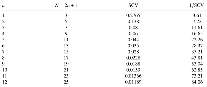
In this section, we discuss the numerical solution of the optimization problem in (6). This numerical optimization can be performed with various optimization methods. For low orders ($n\leq 12$), Wolfram Mathematica can solve this optimization problem in less than 5 min. Table 1 contains the obtained results. The $1/\mathrm {SCV}$ column of the table indicates the minimal order of phase-type distribution needed, to obtain such a low $\mathrm {SCV}$, since the minimal $\mathrm {SCV}$ of an order $N'$ phase-type distribution is $1/N'$. For example, the $\mathrm {SCV}$ of CME-R with order $N=25$ is less than the $\mathrm {SCV}$ of any phase-type distribution of order $N'=84$.

Table 1.

The $\mathrm {SCV}$ and its inverse for low order CME-R.

For higher orders, efficient optimization tools, allowing high precision computation, are required to perform the optimization. In the numerical optimization of the parameters, we had success with evolution strategies. We found the covariance matrix adoption evolution strategy (CMA-ES) [Reference Hansen7] to be the most efficient method for this optimization problem.

More precisely, even more accurate evolution strategy methods, for example, the BIPOP-CMA-ES with restarts [Reference Hansen8] failed to find the global optimum even for low-order cases, because they distribute the $\tau _i$ points on the left and the right of the main peak of $f_n(t)$ suboptimally.

With appropriate initial guess, CMA-ES keeps the number of points left and right to the main peak fixed and optimizes the position of the left and right points much faster than the BIPOP-CMA-ES method. Generally, the $\mathrm {SCV}$ optimized by the CMA-ES method decreased smoothly with increasing order. For the few $\mathrm {SCV}$ values that were out of trend, we repeated the optimization with different initial guess, which resulted in in-trend values in each case.

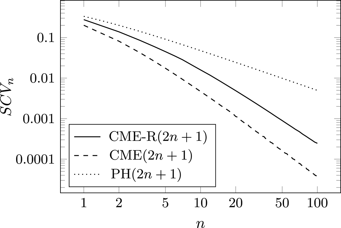
The computation time of the CMA-ES method is around one day at $n=120$. The method provided CME-R distributions with $\mathrm {SCV}$ values as shown in Figure 2. In the figure, the PH$(2n+1)=1/(2n+1)=1/N$ curve represents the minimal $\mathrm {SCV}$ of PH distributions [Reference Aldous and Shepp4], while the dashed line represents the $\mathrm {SCV}$ of matrix exponential distributions with complex eigenvalues (CME) of order $N=2n+1$ [Reference Horváth, Horváth and Telek10].

Figure 2.

The minimal $\mathrm {SCV}$ computed by the CMA-ES method as a function of the order in a log–log scale.

3.1. Required precision of the floating point arithmetic

For higher orders, the computation of the $\mathrm {SCV}$ based on $\tau _1,\ldots ,\tau _n$ might cause numerical issues if the applied floating point arithmetic is not sufficiently accurate. Indeed, the computation of the $a_0,\ldots ,a_{2n}$ coefficients based on (8) and then the computation of the $\mathrm {SCV}$ based on (7) require high precision arithmetic.

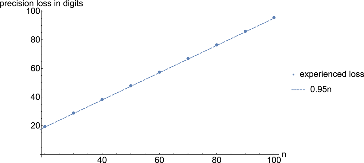
The precision loss in computing the $\mathrm {SCV}$ increases with increasing order, as both the maximum value of the $a_i$ parameters and the $i!$ factorials increases rapidly in (7), but the (unnormalized) moments in (9) increase relatively slowly, because the $a_i$ parameters have alternating sign. Using the Precision function of Mathematica, we made numerical investigations in order to characterize the required floating point arithmetic as a function of the $n$. The results are shown in Figure 3. We found that the precision loss in computing the $\mathrm {SCV}$ is approximately $0.95 n$ digits.

Figure 3.

Precision loss during the computation of the $\mathrm {SCV}$ as a function of the order.

That is, computing the $\mathrm {SCV}$ for $n=100$ (i.e., order $N=201$) results in $95$ digits precision loss, thus to obtain the $\mathrm {SCV}$ in standard double precision the computation of (8) and (7) needs to be performed with extended floating point arithmetic whose precision is $95$ digits larger than the one of double precision. We assume that the number of accurate digits in standard double precision numbers is approximately $20$, and in the implementation of the optimization procedure, for order $2n+1$, we computed the $\mathrm {SCV}$ with $20+0.95n$ digit precision arithmetic.

We note that the input data of this procedure ($\tau _1,\ldots ,\tau _n$) and its results ($\mathrm {SCV}$) need to be represented in only standard double precision.

4. Heuristic optimization

Since the direct applicability of CMA-ES for the optimization of all $\tau _i$ ($i=1,\ldots ,n$) parameters is limited to $n\leq 120$ due to the high number of parameters to optimize, for higher orders we needed to simplify the optimization problem.

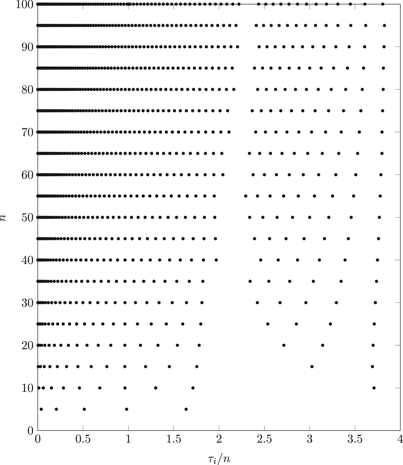
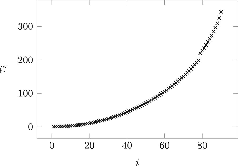
To reduce the complexity of the optimization procedure, first we investigated the location of the optimal $\tau _i$ parameters, which are summarized in Figure 4. According to the figure, the main properties of the optimal $\tau _i$ ($i=1,\ldots ,n$) parameters are as follows:

• • the $\tau _i$ parameters are located in the interval $(0,3.8n)$,

• • the largest gap between the $\tau _i$ parameters represents the main peak of the function and is located at around $2.3n$,

• • the number of $\tau _i$ parameters right of the main peak is gradually increasing with $n$ and it is in the range of $0.1n - 0.2n$,

• • the $\tau _i$ parameters are dense around zero and the distance between the consecutive $\tau _i$ values increases gradually for larger values (aside from the main gap, cf. Figure 5).

Figure 4.

Results of the CMA-ES method, which optimizes $n$ parameters for order $n$. The plot depicts the location of the zeros of $f_n(t)$, denoted by $\tau _i$ ($i=1,\ldots ,n$), normalized by the order for different orders up to $n=100$.

Figure 5.

The optimal location of the zeros of $f_n(t)$ for $n=90$ obtained by the CMA-ES optimization method. The zeros are denoted as $\tau _1,\ldots , \tau _{90}$.

Based on these properties of the $\tau _i$ values, we developed a heuristic optimization procedure which intends to mimic the same properties based on a limited number of parameters.

We approximate the location of the $\tau _i$ parameters with two polynomial curves, one for $\tau _i$ values left to the main peak and one for right to it, which intuition is gained from Figure 5 and related numerical experiments. Thus,

(10)\begin{equation} \tau_i = \left\{ \begin{array}{ll} \theta (i- \phi)^{a}, & \text{if } i\leq i^{*},\\ \Theta (i- \Phi)^{A}, & \text{if } i^{*}< i \leq n, \end{array}\right.\end{equation}

where $i^{*}$ denotes the number of $\tau _i$ parameters left to the main peak and $a$ and $A$ are the shape parameters left and right to the main peak. We could optimize the $i^{*}$, $\theta$, $\Theta$, $\phi$, $\Phi$, $a$, $A$ parameters of the polynomial curves in (10) directly, however we transform the optimization problem to the following set of more expressive parameters: $i^{*}$, $p_{\textrm {min}}$, $p_{\textrm {max}}$, $p$, $w$, $a$, $A$, where $p_{\textrm {min}}$ and $p_{\textrm {max}}$ are the smallest and largest $\tau _i$ parameters, and $p$ and $w$ are the location of the main peak and its width.

The relation between the optimization parameters and the parameters of the polynomial curves are provided by the following equations

(11)\begin{equation} \tau_1 = p_{\textrm{min}},\quad \tau_{i^{*}} = p-w/2,\quad \tau_{i^{*}+1} = p+w/2,\quad \tau_{n}= p_{\textrm{max}}, \end{equation}

where we apply the following constraints:

$$i^{*}< n-1,\quad 0 < p_{\textrm{min}} < p-w/2 < p+w/2 < p_{\textrm{max}},\quad a>0, \quad A>0.$$

Using (10) and (11), we get

(12)\begin{align} \phi & = \frac{(p-w/2)^{1/a} - i^{*} p_{\textrm{min}}^{1/a}}{(p-w/2)^{1/a}-p_{\textrm{min}}^{1/a}} ,\quad \theta=p_{\textrm{min}} (1-\phi)^{{-}a}, \end{align}

(13)\begin{align} \Phi & = \frac{n (p+w/2)^{1/A} - (i^{*}+1) p_{\textrm{max}}^{1/A}}{(p+w/2)^{1/A}-p_{\textrm{max}}^{1/A}} ,\quad \Theta=p_{\textrm{max}} (n-\Phi)^{{-}A}. \end{align}

Applying (12) and (13), the optimization problem modifies to

$$\min_{i^{*},p_{\textrm{min}},p_{\textrm{max}},p,w,a,A}\frac{(\sum_{i=0}^{2n} a_{i} (i+2)!) (\sum_{i=0}^{2n} a_{i} i!)}{(\sum_{i=0}^{2n} a_{i} (i+1)!)^{2}}-1,$$

where $i^{*},p_{\textrm {min}},p_{\textrm {max}},p,w,a,A$ defines $\tau _1, \ldots , \tau _n$ according to (12), (13), and (10) and $\tau _1, \ldots , \tau _n$ defines $a_0,\ldots ,a_{2n}$ according to (8).

The number of parameters of this optimization problem is $7$ for any order $N=2n+1$. For $n>50$, the computational complexity of this heuristic optimization procedure is significantly less than for the CMA-ES method, when optimizing all $\tau _i$ parameters. Due to the reduced complexity of the optimization procedure, we could optimize CME-R distributions for up to $n=5000$.

For order $N=2n+1$, we start the optimization with the following initial values of the parameters, which are good approximates of the optimal parameters according to our numerical experiences.

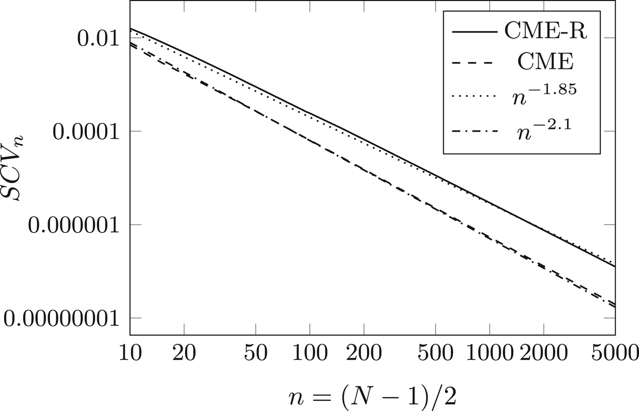
The $\mathrm {SCV}$ values obtained from the $7$ parameter optimization procedure are depicted in Figure 6 for different orders up to $n=5000$. In the figure, the solid line indicates the $\mathrm {SCV}$ values obtained by the CMA-ES optimization of the heuristic (7 parameter) procedure. To demonstrate the decay of the $\mathrm {SCV}$ values, the $n^{-1.85}$ curve is plotted next to it. The decay of the CME-R curve drops below the $n^{-1.85}$ curve at $n=2000$ and decays faster from that point on. Additionally, the figure contains the CME curve, which is the $\mathrm {SCV}$ of the concentrated matrix exponential distribution with complex eigenvalues and its supporting decay curve $n^{-2.1}$. At $n=2000$, the $\mathrm {SCV}$ of the CME distribution is one order of magnitude smaller than the $\mathrm {SCV}$ of the CME-R distribution.

Figure 6.

The minimal $\mathrm {SCV}$ of the CME and the CME-R distributions of order $n$ as a function of $n$ in a log–log scale. To indicate the decay rates, the $n^{-1.85}$ and the $n^{-2.1}$ curves are plotted as well.

5. Numerical ILT with CME-R

In this section, we discuss the application of CME-R for NILT in the Abate–Whitt framework [Reference Abate and Whitt1]. The Laplace transform of a real- or complex-valued function $h(t)$ is defined as

$$h^{*}(s)=\int_{t=0}^{\infty}e^{{-}st}h(t)\,\mathrm{d}t.$$

The goal of NILT is to obtain $h(t)$ from $h^{*}(s)$. The NILT methods in the Abate–Whitt framework use the approximation

(14)\begin{equation} h(T)\approx \sum_{k=1}^{M}\frac{\eta_k}{T}h^{*}\left(\frac{\beta_k}{T}\right), \end{equation}

where $\eta _k$ and $\beta _k$ are real or complex numbers that depend on $M$, but not on the transform function $h^{*}$ or the argument $T$. $M$ is called the order of the approximation, and indicates the number of $h^{*}$ evaluations needed to calculate the ILT.

The Abate–Whitt framework has an integral-based interpretation [Reference Horváth, Horváth, Al-Deen Almousa and Telek9] using that

(15)\begin{align} h(T) & \approx \sum_{k=1}^{M}\frac{\eta_k}{T}h^{*}\left(\frac{\beta_k}{T}\right) =\sum_{k=1}^{M}\frac{\eta_k}{T}\int_{t=0}^{\infty}e^{-({\beta_k}/{T})t}h(t)\,\mathrm{d}t\nonumber\\ & =\sum_{k=1}^{M}\frac{\eta_k}{T}\int_{t=0}^{\infty}e^{-({\beta_k}/{T})t}h(t)\,\mathrm{d}t =\int_{t=0}^{\infty}h(tT)\sum_{k=1}^{M}\eta_k e^{-\beta_k t}\,\mathrm{d}t\nonumber\\ & =\int_{t=0}^{\infty}h(tT)g_M(t)\,\mathrm{d}t, \end{align}

where

(16)\begin{equation} g_M(t)=\sum_{k=1}^{M}\eta_k e^{-\beta_k t}. \end{equation}

If $g_M(t)$ was the Dirac impulse at $t=1$, then (15) would provide $h(T)$ exactly. When $g_M(t)$ is a good approximate of the Dirac impulse, we assume that (15) closely approximates $h(T)$.

Similar to [Reference Horváth, Horváth, Al-Deen Almousa and Telek9], using the fact that $g_M(t)$ is non-negative, we measure the quality of the approximation of the Dirac impulse function with the $\mathrm {SCV}$ of $g_M(t)$. The $\mathrm {SCV}$ of the Dirac impulse is $0$, therefore we assume that the lower the $\mathrm {SCV}$ of $g_M(t)$, the better it approximates the Dirac impulse function.

As it is discussed in the previous section, the pdf of CME-R is

(17)\begin{equation} f_n(t)= c \prod_{i=1}^{n} (\lambda t-\tau_i)^{2} e^{-\lambda t} = \sum_{i=0}^{2n} a_{i} t^{i} e^{-\lambda t}. \end{equation}

Assuming that $c$ and $\lambda$ are set such that $\mu _0=\mu _1=1$, the above pdf is concentrated around $1$. Additionally, the $\mathrm {SCV}$ of $f_n(t)$ can be set to be low, in which case $f_n(t)$ is a close approximate of the Dirac impulse.

To apply CME-R distributions for NILT in the Abate–Whitt framework according to (14), we still need to approximate $f_n(t)$ (defined in (17)) with $g_M(t)$ (defined in (16)) such that the $\eta _j$ and $\beta _j$ parameters are real.

To this end, we set the $\beta _j$ parameters to be equidistant around $\lambda$ and set the $\eta _j$ parameters such that the set of the first $M$ coefficients of the Taylor series of $f_n(t)$ and $g_M(t)$ are identical.

That is, for $-m\leq j \leq m$, we choose $\beta _j=\lambda +j \delta$ and solve

(18)\begin{equation} \textrm{Taylor}(t^{i} e^{-\lambda t},2m+1) = \textrm{Taylor}\left(\sum_{j={-}m}^{m} \nu_{ij} e^{-(\lambda+j \delta) t},2m+1\right) \end{equation}

for the unknowns $\nu _{ij}$. In (18), the $n$th coefficient of the Taylor series of $f(t)$ is $\lim _{t\to 0} ({d^{n}}/{dt^{n}}) ({f(t)}/{n!})$ and $\textrm {Taylor}(f(t),k)$ denotes the vector of the $\{0,1,\ldots , k\}$ coefficients of the Taylor series of $f(t)$.

It is worth noting that the $\nu _{ij}$ coefficients, computed according to (18), are in close connection with the finite difference coefficients from numerical differentiation [Reference Keller and Pereyra11], as $\nu _{ij}={c_{ij}}/{(-\delta )^{i}}$, where $c_{ij}$ are the aforementioned finite difference coefficients. The problem of approximating $f_{n}(t)$ in (17) in the form of $g_M(t)$ in (16) can be formulated using Laplace transformation and the finite difference method as it is shown in the Appendix.

Based on $t^{i} e^{-\lambda t} \approx \sum _{j=-m}^{m} \nu _{ij} e^{-(\lambda +j \delta ) t}$, we have

(19)\begin{equation} f_n(t)=\sum_{i=0}^{2n} a_{i} t^{i} e^{-\lambda t} \approx \sum_{j={-}m}^{m} \sum_{i=0}^{2n} a_{i} \nu_{ij} e^{-(\lambda+j \delta) t} = \sum_{j={-}m}^{m} \eta_j e^{-\beta_j t} \triangleq f_{m,n}(t), \end{equation}

with

(20)\begin{equation} \eta_j=\sum_{i=0}^{2n} a_{i}\nu_{ij}=\sum_{i=0}^{2n} \frac{a_{i} c_{ij}}{(-\delta)^{i}} \quad \text{and}\quad \beta_j=\lambda+j \delta. \end{equation}

That is, $f_{m,n}(t)$ is the order $m$ approximation of the order $n$ CME-R distribution $f_n(t)$.

The $f_{m,n}(t)$ expression is in the form (16), which allows the application of the Abate–Whitt NILT framework according to

(21)\begin{equation} h(T) \approx h_{m,n}(T) = \sum_{j={-}m}^{m} \frac{\eta_j}{T} h^{*}\left(\frac{\beta_j}{T}\right) . \end{equation}

The order of the NILT approximation is $M=2m+1$, that is, we need to evaluate $h^{*}(s)$ in $2m+1$ real points to obtain $h_{m,n}(t)$.

A possible setting of parameter $\delta$ is, for example, $\delta = {\lambda }/{20 m}$, which means that $\beta _j\in [0.95\lambda ,1.05\lambda ]$. According to our numerical investigations, $m \approx 1.3n$ gives an accurate approximation of the derivatives in this case. The effect of these parameters are discussed below, and the consideration about the numerical precision of the computations in the next section, is obtained using this setting of $\delta$ and $m$.

5.2. Accuracy of the NILT procedure

Approximating $h(T)$ by $h_{m,n}(T)$ contains two approximation errors, since $h(T)\approx h_{n}(T)$ and $h_n(T)\approx h_{m,n}(T)$, where $h_n(T) \triangleq \int _{t=0}^{\infty } h(t T) f_n(t) \,\mathrm {d}t$. The difference between $h(T)$ and $h_n(T)$ is due to the fact that $f_n(t)$ (the pdf of the chosen CME-R) differs from the Dirac impulse. We can measure the accuracy of this approximation independent of $h(T)$ using the $\mathrm {SCV}$ of $f_n(t)$. As discussed in Section 4, the $\mathrm {SCV}$ of $f_n(t)$ changes according to $n^{-1.85}$. The exact values of the $\mathrm {SCV}$ for $n=1,\ldots ,12$ are given in Table 1 and for higher orders in Figure 6.

The difference between $h_n(T)$ and $h_{m,n}(T)$ is due to the approximation of $f_n(t)$ by $f_{m,n}(t)$. Since $f_n(t)$ is such that $\int _t f_{n}(t) \,\mathrm {d}t=\int _t t f_{n}(t) \,\mathrm {d}t=1$, we used $|\int _t t f_{m,n}(t) \,\mathrm {d}t-1|$ as an error measure of the approximation and considered $|\int _t t f_{m,n}(t) \,\mathrm {d}t-1|<10^{-4}$ to be appropriate accuracy for the $h_n(T)\approx h_{m,n}(T)$ approximation. For a given $n$, the accuracy of the $h_n(T)\approx h_{m,n}(T)$ approximation is determined by $\delta$ and $m$. According to our numerical experiences, for fixed $n$ and $\delta$, the modification of $m$ has two contradicting effects. When $m$ increases, the $|\int _t t f_{m,n}(t) \,\mathrm {d}t-1|$ measure of the error decreases, but the precision loss of the computation increases.

The choice of $\delta$ is also a trade-off. A lower $\delta$ value requires a lower $m/n$ ratio, which means a more efficient NILT, because the order of the NILT is $M=2m+1$ (the Laplace transform function needs to be evaluated in $2m+1$ points), while the $\mathrm {SCV}$ of $f_{m,n}(t)$ is characterized by $n$. That is, decreasing $\delta$ is beneficial for efficient NILT, but using a lower $\delta$ value also increases the numerical precision loss.

Since the quantitative effect of $m$ and $\delta$ depends on multiple factors, we used numerical investigations to determine the highest $\delta$ value that provides the required accuracy ($|\int _t t f_{m,n}(t) \,\mathrm {d}t-1|<10^{-4}$). Table 2 summarizes the results. Our numerical investigations indicate that for a given $m$ value the best choice of $\delta$ is the one provided in the table, because using a lower $m$ violates the $|\int _t t f_{m,n}(t) \,\mathrm {d}t-1|<10^{-4}$ inequality and consequently the $h_n(T)\approx h_{m,n}(T)$ approximation is poor, while using larger $\delta$ increases precision loss, thus the required precision exceeds the values reported in the previous section.

Table 2.

The required number of points and their distances for accurate derivative approximation. The derivative approximation is assumed to be accurate when $|\int _t t f_{m,n}(t) \,\mathrm {d}t-1|<10^{-4}.$

Our recommended values of the parameters, $\delta = {\lambda }/{20 m}$ and $m \approx 1.3n$, offer a potential compromise between efficiency and precision loss.

6. Numerical experiments

To investigate the properties of the proposed NILT method using CME-R, we compared it with other methods of the Abate–Whitt framework, namely the CME [Reference Horváth, Horváth, Al-Deen Almousa and Telek9], Euler [Reference Abate, Choudhury and Whitt2], and Gaver–Stehfest [Reference Stehfest14] methods. The CME method is an obvious choice, as the proposed method can be thought of as its real eigenvalue counterpart. The Euler method was chosen since, aside from the CME method, it had the best overall performance in the tests of [Reference Horváth, Horváth, Al-Deen Almousa and Telek9]. Finally, the Gaver–Stehfest method (referred to as the Gaver method in the following) was included because, unlike the CME and Euler method (and similar to the CME-R method) it can be implemented using real arithmetic. A short summary of these methods can be found in [Reference Horváth, Horváth, Al-Deen Almousa and Telek9].

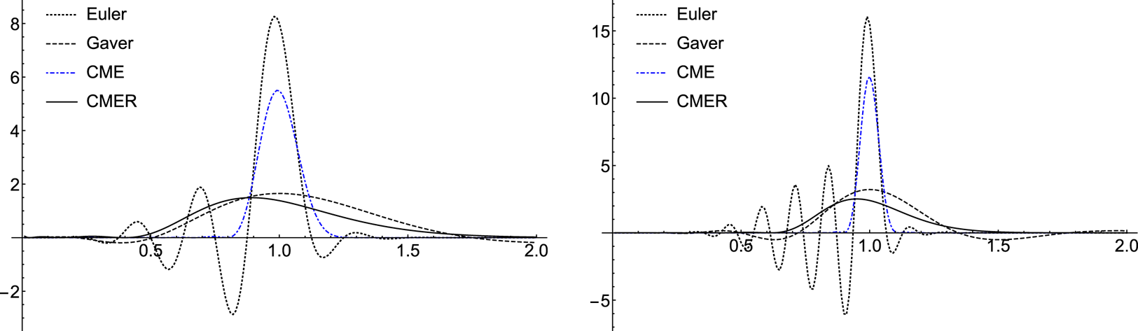
First, in Figure 7, we examine the $g_M(t)$ functions (defined in (16)) corresponding to the different NILT methods, to assess some of their characteristics. In each of the Abate–Whitt framework methods, if $g_M(t)$ approximates the Diract impulse at $t=1$ well, then we expect the NILT method to provide a close approximation of $h(t)$. Figure 7 shows that the main peak of the Euler and Gaver methods is more concentrated than that of the CME and CME-R methods, respectively. On the other hand, contrary to the CME and CME-R methods, the $g_M(t)$ of the Euler and Gaver methods oscillate heavily and have high negative peaks, which leads to Gibbs oscillation for $h(t)$ functions with discontinuity. A more in-depth discussion of these characteristics and their consequences can be found in [Reference Horváth, Horváth, Al-Deen Almousa and Telek9].

Figure 7.

The $g_{M}(t)$ function of the CME-R method, which intends to approximating the Dirac impulse function and the associated functions of the Euler, Gaver, and CME methods for order $10$ and $20$.

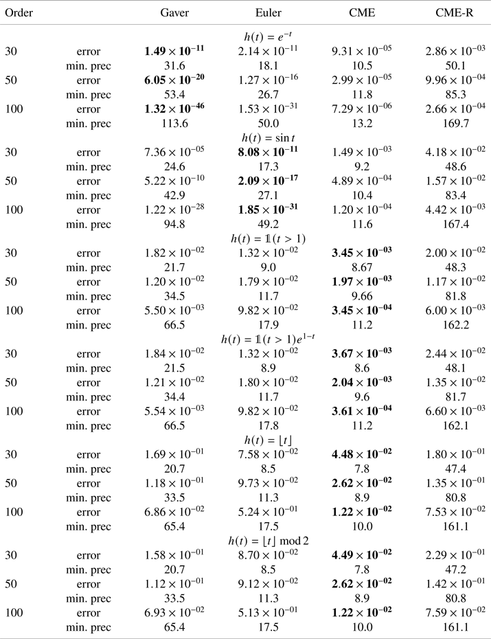
To compare the previously mentioned NILT methods, we performed NILT using the above methods with orders $M=30$, 50, 100 on the functions in Table 3. We considered two performance metrics: the 1-norm of the error of the NILT over the $[0,T]$ time interval, and the required numerical precision in digits for the calculations. To approximate the 1-norm of the error, we used that

(22)\begin{equation} e_1=\|h-h_n\|_1=\int_0^{T} |h(t)-h_n(t)|\,\mathrm{d}t\approx \frac{1}{K}\sum_{k=1}^{K} \left|h\left(\frac{kT}K\right)-h_n\left(\frac{kT}K\right)\right|, \end{equation}

where $h(t)$ is the original time domain function and $h_n(t)$ is its NILT approximation. We used $T=5$ for the interval and $K=100$ points to approximate the integral.

Table 3.

The set of test functions used for the numerical evaluation of the NILT methods.

To evaluate the required precision, we determined what is the $p_{\textrm {min}}$ minimal precision which guarantees that the error of the calculation is affected only by the error of the NILT method and not by the numerical precision. To do so, we performed the calculations with a sufficiently high $p_{\textrm {calc}}$ initial precision, and for every NILT method and order we subtracted from it the $p_{\textrm {norm}}$ precision of the 1-norm error, that is,

$$p_{\textrm{min}}=p_{\textrm{calc}}-p_{\textrm{norm}}+2,$$

where the extra two digits ensure that the first two digits of the 1-norm error are accurate. The results of the NILT computations can be found in Table 4. We can see that for smooth functions ($e^{-t}$, $\sin {t}$, i.e., those without discontinuity), the Gaver and the Euler method have the lowest 1-norm error (indicated by boldface numbers), and it also decreases rapidly with increasing order. The CME and the CME-R method are significantly worse in this regard, but if extremely high accuracy is not required, both are usable alternatives. For functions with discontinuity, the CME method gives the lowest 1-norm error, the Gaver and the CME-R method have similar performance, while the Euler method has slightly smaller error than the Gaver and CME-R methods for smaller orders, but the error increases for higher orders.

Table 4.

1-norm error of the ILT methods for the test functions.

For every computation, the CME method requires the lowest precision. When using the CME method, standard double precision is always sufficient in the examined cases. The Euler method has slightly higher precision requirements. It can be applied using double precision for moderate orders—if extremely high accuracy is not required. If we want to attain high accuracy (e.g., $10^{-16}$ for $h(t)=e^{-t}$ with order 50 NILT), naturally, we need to apply the appropriately high precision, as shown in Table 4. Double precision is not enough in case of the Gaver method, not even for lower orders. The required precision is around 20–30 digits for order $10$ and 60–70 digits for order $100$ NILT, even if only lower accuracy is needed. The CME-R method demands the highest precision: approximately $50$ digits for order $10$ and as high as $170$ digits for order $100$ NILT.

Based on the above, the CME method is the best overall NILT method, but the Euler method can be used with lower error, if it is known that the time domain function is smooth. However, both require complex arithmetic and the ability to evaluate the Laplace domain function in complex points. If only real arithmetic is available, or the Laplace domain function cannot be evaluated in complex points, then the Gaver method is more efficient than the CME-R method, because it requires lower precision and has smaller error for smooth functions. The CME-R method should be used if the CME and Euler methods cannot be used, and we want to avoid overshoot.