1 Introduction
The trajectory of a steady jet in cross-flow has been widely studied in the literature (for an overview see reviews by Margason (Reference Margason1993) and Mahesh (Reference Mahesh2013)). When the jet is forced or pulsed at a fixed frequency, its trajectory can be altered significantly (Vermeulen, Chin & Yu Reference Vermeulen, Chin and Yu1990). While the scaling of the trajectory with jet velocity is fairly well established, the scaling of trajectory with frequency has not been studied in detail in the literature. Three cases are considered here in which a jet in cross-flow is subjected to a frequency component: a forced jet in which a periodic variation is imposed on a non-zero mean jet velocity, a pulsed jet in which discrete pulses of the jet are alternated with zero velocity between pulses, and a synthetic jet in which equal blowing and suction pulses are alternated leading to a zero-net-mass-flux flow at the jet exit but a train of blowing pulses away from the jet exit. In the following, these three cases are generalized using the term ‘unsteady jet’. The velocity cycle of such an unsteady jet can be generalized as
 $u_{j}(t)=\langle u_{j}\rangle +u_{j}^{\prime }(t/T)$
, where
 $\langle u_{j}\rangle$
represents the time-averaged jet velocity and
 $u_{j}^{\prime }$
the cyclic fluctuations around this average with frequency
 $f=1/T$
. When using sinusoidal forcing as in the present study, the velocity cycle is described by
 $$\begin{eqnarray}u_{j}(t)=\langle u_{j}\rangle +u_{j}^{\prime }\sin (2\unicode[STIX]{x03C0}tf).\end{eqnarray}$$
The forced jet is the most general case, with usually
 $\langle u_{j}\rangle >u_{j}^{\prime }$
, while the pulsed and synthetic jets are special cases, where
 $\langle u_{j}\rangle =u_{j}^{\prime }$
for pulsed jets, and
 $\langle u_{j}\rangle =0$
for synthetic jets. (Note that forced and pulsed jets are generally driven by a square wave instead of a sinusoidal wave.) These three cases have some clear differences (especially between blowing pulses, where
 $u_{j}>0$
for forced jets,
 $u_{j}=0$
for pulsed jets and
 $u_{j}<0$
for synthetic jets) but also have significant similarity in that coherent vortical structures are formed with the specified frequency (see for example Wu, Vakili & Yu (Reference Wu, Vakili and Yu1988) for forced jets, Eroglu & Breidenthal (Reference Eroglu and Breidenthal2001) for pulsed jets and Jabbal & Zhong (Reference Jabbal and Zhong2008) for synthetic jets). It has been suggested that variations in the trajectory are related to the distance between these vortical structures (Eroglu & Breidenthal Reference Eroglu and Breidenthal2001; Jabbal & Zhong Reference Jabbal and Zhong2010). If so, scaling of the trajectory with frequency might be analogous between the three unsteady jet cases. The present study focuses on deriving this scaling by fitting empirical data of a synthetic jet in a turbulent boundary layer.
Applications of unsteady jets in cross-flow include control of the jet in cross-flow (Narayanan, Barooah & Cohen Reference Narayanan, Barooah and Cohen2003), separation control (Dandois, Garnier & Sagaut Reference Dandois, Garnier and Sagaut2007), thrust vector control (Miller et al. Reference Miller, Yagle, Bender and Smith2001), film cooling (Muldoon & Acharya Reference Muldoon and Acharya2009) and skin-friction control. Recent results have shown that skin-friction drag can be reduced up to 3 % by targeting the large-scale structures of a high-Reynolds-number turbulent boundary layer using a pulsed jet (Abbassi et al. Reference Abbassi, Baars, Hutchins and Marusic2017). In similar experiments, the near-wall structures of a turbulent boundary layer were targeted using a synthetic jet (Rathnasingham & Breuer Reference Rathnasingham and Breuer2003). A common feature in these studies is the rectangular orifice shape flush with the wall and aligned with the long dimension in streamwise direction, analogous to the orientation of near-wall streaks and large-scale structures in the turbulent boundary layer. In these control studies, incoming structures in the flow are detected upstream of the orifice, upon which the jet is fired to target these structures. For the efficient targeting of structures away from the wall it is important to know the trajectory of the jet. The present study is motivated by the application of skin-friction control, which is reflected in the rectangular orifice geometry and the low ratio of jet velocity to cross-flow velocity compared to some other studies (this is required for the jet to stay inside the boundary layer).
In addition to the trajectory of a jet, spread (Davitian et al. Reference Davitian, Hendrickson, M’Closkey and Karagozian2010), mixing (Smith & Mungal Reference Smith and Mungal1998), entrainment (Narayanan et al. Reference Narayanan, Barooah and Cohen2003), bifurcation (Eroglu & Breidenthal Reference Eroglu and Breidenthal2001) and shear-layer instabilities (Megerian et al. Reference Megerian, Davitian, Alves and Karagozian2007) are important factors in the development of a jet in cross-flow (Mahesh Reference Mahesh2013; Karagozian Reference Karagozian2014). Given the stated motivation of targeting structures in the flow, the present study focuses on the trajectory only. Note that bifurcation of the jet has not been observed in the present study and the trajectory consists of a single branch.
The remainder of this introduction starts with a description of the canonical case: a steady circular jet issuing in a uniform cross-flow. This is followed by a discussion of the effect of an actuation frequency (i.e. an unsteady jet). Next, the influence of changing the orifice shape (rectangular instead of circular) is examined and some considerations for an orifice length scale are presented. Then, the influence of issuing into turbulent boundary layers (as opposed to laminar boundary layers or a uniform cross-flow) is discussed. Finally, the important parameters are summarized and scaling parameters are proposed that describe the influence of the mentioned aspects on the trajectory.
1.1 Canonical case: steady circular jet
The canonical case for the jet in cross-flow is a steady circular jet in a uniform cross-flow (Johari Reference Johari2006; Mahesh Reference Mahesh2013). Jet trajectories are typically normalized by a relevant orifice length scale
 $D$
(usually the diameter for circular jets) and the velocity ratio between the jet and the free-stream velocities,
 $r=u_{j}/U_{\infty }$
. For example, Broadwell & Breidenthal (Reference Broadwell and Breidenthal1984) derived a scaling
 $rD$
based on the jet as point source of momentum, while Karagozian (Reference Karagozian1986) derived a scaling including viscous effects which can be expressed as
 $r^{1.7}D$
and Keffer & Baines (Reference Keffer and Baines1962) found a collapse of their data for
 $r^{2}D$
. Using a generalized scaling of
 $r^{c}D$
, the trajectory of a jet in cross-flow is usually described by an empirical power law of the form
 $$\begin{eqnarray}\frac{y}{r^{c}D}=B\left(\frac{x}{r^{c}D}\right)^{n},\end{eqnarray}$$
where
 $y$
is the wall-normal location,
 $x$
is the streamwise location and
 $B$
,
 $n$
and
 $c$
are constants. A comparison by Mahesh (Reference Mahesh2013), considering different studies, shows that trajectories do not fully collapse when normalized by
 $rD$
, indicating that
 $B$
,
 $n$
and
 $c$
are not constant. Indeed, ranges are reported of
 $1.2<B<2.6$
,
 $0.28<n<0.34$
and
 $0<c<2$
(Mahesh Reference Mahesh2013). Although most authors define the trajectory using a single scaling, Smith & Mungal (Reference Smith and Mungal1998) defined three regions of the transverse jet, each with a different length scale: a vortex interaction region just downstream of the orifice scaling with
 $D$
, a near field scaling with
 $rD$
, and a far field scaling with
 $r^{2}D$
. Broadwell & Breidenthal (Reference Broadwell and Breidenthal1984) defined a far field as the region where structures created by the jet move with the cross-flow velocity, limited by
 $x\gg r\sqrt{\unicode[STIX]{x03C0}D^{2}/4}$
. Using this definition, the low velocity ratios used in the present study cause all measurements to be performed in the far field.
The development of a jet in cross-flow can be (inadequately) described in terms of momentum fluxes by decomposing the trajectory into a wall-normal and a streamwise part. The wall-normal development (or penetration) of the jet is dominated by the momentum flux created by the jet at the orifice. As the jet penetrates into the cross-flow, the initial wall-normal momentum decreases due to drag. At the same time, the cross-flow transfers streamwise momentum to the jet, accelerating the jet until the cross-flow velocity is reached. This combination causes the trajectory to evolve from pointing in the wall-normal direction at the orifice to pointing in the streamwise direction in the far field.
The above analysis leads to an incomplete description of the jet, since the interaction with the cross-flow leads to a complex set of coherent vortical structures (Fric & Roshko Reference Fric and Roshko1994). The cross-section of a jet in cross-flow is dominated by a counter-rotating vortex pair (e.g. Karagozian Reference Karagozian2014). This vortex pair creates a self-induced velocity on the jet in the vertical direction, influencing the trajectory. In the far field where the initial wall-normal momentum has decayed, the velocity induced by this vortex pair is shown to drive the wall-normal penetration (Broadwell & Breidenthal Reference Broadwell and Breidenthal1984). In fact, multiple theoretical descriptions of the trajectory have been derived based on the strength and induced velocity of this counter-rotating vortex pair (e.g. Broadwell & Breidenthal Reference Broadwell and Breidenthal1984; Karagozian Reference Karagozian1986).
1.2 Unsteady jets
It may be assumed that for unsteady jets the velocity induced by created vortical structures has an equally important effect on the trajectory. Johari (Reference Johari2006) derived scaling parameters for the penetration of isolated vortex rings into a cross-flow. These parameters are based on the impulse of the vortex ring (directly related to the circulation) and ultimately lead to a scaling of the trajectory with the non-dimensional stroke length which represents the length of the slug of fluid ejected each pulse and is related to the optimal formation of vortex rings (Gharib, Rambod & Shariff Reference Gharib, Rambod and Shariff1998). However, in most cases the interaction between an unsteady jet and a cross-flow does not produce isolated vortex rings but a train of non-trivial vortical structures that interact with each other. Jabbal & Zhong (Reference Jabbal and Zhong2010) showed that the trajectory of synthetic jets in a cross-flow depends on the type of vortical structures created by the jet. Depending on the velocity ratio and non-dimensional frequency, the interaction of a pulsed or synthetic jet with a cross-flow can lead to vortical structures such as tilted, distorted and stretched vortex rings or hairpin vortices (Jabbal & Zhong Reference Jabbal and Zhong2008; Sau & Mahesh Reference Sau and Mahesh2008). The velocity induced by a single vortical structure depends on the circulation and the geometry of the structure. In addition, for a train of vortical structures as created by a forced, pulsed or synthetic jet, the spacing and interaction between vortical structures also play an important role (Eroglu & Breidenthal Reference Eroglu and Breidenthal2001; Jabbal & Zhong Reference Jabbal and Zhong2010). Owing to the interaction with the cross-flow boundary layer, the circulation (partially cancelled by the shear in the cross-flow) and geometry of these structures are non-trivial functions of the actuation and cross-flow parameters. This implies that theoretical scalings for the trajectory such as derived by Broadwell & Breidenthal (Reference Broadwell and Breidenthal1984) and Karagozian (Reference Karagozian1986) for a counter-rotating vortex pair or by Johari (Reference Johari2006) for isolated vortex rings would be highly dependent on these parameters for an unsteady jet in a cross-flow. Therefore, theoretical scaling laws are hard to formulate when such geometrically complicated vortical structures are formed. The present work does not consider the exact mechanisms in which the actuation and cross-flow parameters influence the trajectory, but rather investigates the variation and scaling of the trajectory with these parameters.
The trajectory of an unsteady jet is generally described using (1.2) (e.g. Eroglu & Breidenthal Reference Eroglu and Breidenthal2001; Smith Reference Smith2002), which is independent of actuation frequency. However, as discussed above and shown in numerous studies (e.g. Vermeulen et al. Reference Vermeulen, Chin and Yu1990; Johari, Pacheco-Tougas & Hermanson Reference Johari, Pacheco-Tougas and Hermanson1999; Eroglu & Breidenthal Reference Eroglu and Breidenthal2001; M’Closkey et al. Reference M’Closkey, King, Cortelezzi and Karagozian2002; Shuster et al. Reference Shuster, Pink, McEligot and Smith2005; Johari Reference Johari2006; Shapiro et al. Reference Shapiro, King, M’Closkey and Karagozian2006), the frequency of an unsteady jet plays an important role in the trajectory through the geometry of the created structures, the circulation of each structure and the distance between subsequent structures. It has to be noted that some studies argue that the duty cycle and pulse width (for square-wave excitation of a forced jet) are more important parameters than the actuation frequency (Shapiro et al. Reference Shapiro, King, M’Closkey and Karagozian2006). Associated time scales are linked to the non-dimensional stroke length for vortex-ring formation (Gharib et al. Reference Gharib, Rambod and Shariff1998) and to shear-layer instabilities (see the recent review by Karagozian (Reference Karagozian2014)). For the present study on synthetic jets with a sinusoidal waveform, the duty cycle is fixed to 0.5 and the pulse width is a direct function of the frequency. Care should be taken when comparing the results of the present study to studies using square-wave forcing, especially when duty cycles other than 0.5 are considered.
In addition to the direct effect of frequency, an important aspect of an unsteady jet is the fluctuating velocity ratio
 $u_{j}(t)/U_{\infty }$
. Usually a single velocity magnitude is defined for the jet, which can be based on the time-averaged jet velocity
 $\langle u_{j}(t)\rangle$
(e.g. Karagozian Reference Karagozian2014), time-averaged momentum flow velocity
 $U_{0}$
(e.g. Eroglu & Breidenthal Reference Eroglu and Breidenthal2001; Cater & Soria Reference Cater and Soria2002) or mean velocity of the blowing part of the cycle
 $\bar{u}$
(e.g. Smith & Glezer Reference Smith and Glezer1998; Johari Reference Johari2006). For a sinusoidal velocity cycle with
 $\langle u_{j}(t)\rangle =0$
(i.e. a synthetic jet) and a constant orifice area, the momentum flow velocity and mean blowing velocity are given by
 $U_{0}=u_{j}^{\prime }/\sqrt{2}$
and
 $\bar{u}=u_{j}^{\prime }/\unicode[STIX]{x03C0}$
, respectively (with
 $u_{j}^{\prime }$
as defined in (1.1)), i.e.
 $U_{0}=\bar{u}\unicode[STIX]{x03C0}/\sqrt{2}$
. Following a large body of literature on synthetic jets, the present study characterizes the jet using the mean blowing velocity (Smith & Glezer Reference Smith and Glezer1998). Using this velocity magnitude, the waveform of a sinusoidal synthetic jet is fully described by the velocity magnitude
 $\bar{u}$
and frequency
 $f$
. The velocity ratio is then defined as
 $$\begin{eqnarray}r=\bar{u}/U_{\infty }.\end{eqnarray}$$
It should be noted that the comparison to a steady jet and other types of unsteady jets might be more appropriate based on the time-averaged momentum of the jet
 $U_{0}$
(Van Buren & Amitay Reference Van Buren and Amitay2016). Any discrepancy is expected to appear in the constants
 $B$
in (1.2) and
 $A$
in (1.6). Neither of these constants influence the scaling investigated in the present study.
1.3 Orifice length scale
In addition to the discussed complicated effect of frequency, the present study differs from the canonical case by using a rectangular orifice shape. This orifice has a constant length
 $l$
and width
 $d$
and is described by the aspect ratio
 $$\begin{eqnarray}AR=l/d.\end{eqnarray}$$
The relevant orifice length scale
 $D$
as appearing in (1.2), which is usually taken to be the diameter of a circular orifice, now needs to be based on the dimensions of a rectangular orifice. Broadwell & Breidenthal (Reference Broadwell and Breidenthal1984) treated the jet as a point source of momentum, leading to a length scale equal to the square root of the cross-sectional area of the orifice, which is proportional to the diameter for a circular orifice and is given by
 $(ld)^{1/2}$
for a rectangular orifice. O’Farrell & Dabiri (Reference O’Farrell and Dabiri2014) showed that the equivalent diameter, also scaling with
 $(ld)^{1/2}$
, is the relevant length scale for formation of vortex rings from rectangular orifices in quiescent flow. These arguments suggest an orifice length scale of
 $D=(ld)^{1/2}$
. However, Van Buren et al. (Reference Van Buren, Leong, Whalen and Amitay2016) showed an influence of the orientation of a rectangular orifice compared to the flow. A synthetic jet actuator with a rectangular orifice of aspect ratio
 $AR=18$
was placed in a cross-flow with the long dimension of the slot aligned in either the spanwise or the streamwise direction. They show that this has a significant effect both on the type of structures created by the jet and on the trajectory, ruling out a length scale of
 $(ld)^{1/2}$
which is independent of orientation. The discrepancy with the scaling derived by Broadwell & Breidenthal (Reference Broadwell and Breidenthal1984) can be explained by the deviation from a point source of momentum when placing a rectangular orifice with the long dimension perpendicular to the cross-flow. This will cause the cross-flow to impact on a relatively large surface of the jet, which is not accounted for by the point-source approach.
Another candidate for the relevant orifice length scale could be the length of the slot in the streamwise direction. However, this dimension is independent of the aspect ratio of the slot, which has been shown to be an important parameter for vortex formation (Van Buren, Whalen & Amitay Reference Van Buren, Whalen and Amitay2014). Moreover, the streamwise length
 $l$
of a slot is the same as the streamwise length of a circular orifice with diameter
 $l$
, while these have been shown to have a very different influence on the flow field (Kim, Kim & Jung Reference Kim, Kim and Jung2012). The same arguments rule out the length of the slot in the spanwise direction as the relevant length scale.
The relevant orifice length scale for scaling of the trajectory using a rectangular orifice is not explored in the literature. While being equal to the diameter for a circular orifice, for a rectangular orifice this length scale depends on the slot width, slot length and orientation compared to the cross-flow. The present study uses a fixed orifice geometry and orientation (based on the skin-friction control motivation discussed above) which does not give any insight into the nature of this relevant length scale. However, it may be assumed that the constant orifice geometry leads to a constant length scale
 $D$
and the results for scaling of the actuation frequency are assumed to be independent of this length scale. The nature of
 $D$
is outside the scope of this current study and we use an arbitrary value of
 $D=1~\text{m}$
where quantification is required.
1.4 Turbulent boundary layer
The present study investigates the trajectory of a rectangular synthetic jet issuing into different turbulent boundary layers. The turbulent boundary layers are characterized using the free-stream velocity
 $U_{\infty }$
, the boundary-layer thickness
 $\unicode[STIX]{x1D6FF}$
, the kinematic viscosity
 $\unicode[STIX]{x1D708}$
and the skin-friction velocity
 $U_{\unicode[STIX]{x1D70F}}$
. It should be noted that the friction velocity is directly related to the free-stream velocity through the skin-friction coefficient
 $c_{f}=2U_{\unicode[STIX]{x1D70F}}^{2}/U_{\infty }^{2}$
, which is a function of
 $\text{log}(Re_{x})$
. For the high values of
 $Re_{x}$
used in the present study (required for high-Reynolds-number turbulent boundary layers),
 $\text{log}(Re_{x})$
is relatively constant, leading to a fixed ratio between
 $U_{\unicode[STIX]{x1D70F}}$
and
 $U_{\infty }$
. Therefore, the free-stream velocity and friction velocity are not varied independently in the present study. The governing non-dimensional parameter describing a turbulent boundary layer is the friction Reynolds number (e.g. Klewicki Reference Klewicki2010; Marusic, Mathis & Hutchins Reference Marusic, Mathis and Hutchins2010; Smits, McKeon & Marusic Reference Smits, McKeon and Marusic2011), defined by
 $$\begin{eqnarray}Re_{\unicode[STIX]{x1D70F}}=U_{\unicode[STIX]{x1D70F}}\unicode[STIX]{x1D6FF}/\unicode[STIX]{x1D708}.\end{eqnarray}$$
This Reynolds number can be interpreted as the ratio between the two characteristic length scales in a turbulent boundary layer: the inner length scale
 $\unicode[STIX]{x1D708}/U_{\unicode[STIX]{x1D70F}}$
and the outer length scale
 $\unicode[STIX]{x1D6FF}$
.
Muppidi & Mahesh (Reference Muppidi and Mahesh2005) studied the influence of the boundary-layer thickness on the trajectory of a steady jet. The main influence identified by these authors was the wall-normal variation of cross-flow velocity in the boundary layer, leading to different (local) values of the velocity ratio.
An additional influence of the turbulent boundary layer is the distribution of vorticity in the cross-flow. It has been shown that the vorticity in the boundary layer (partially) cancels the vorticity in the upstream side of vortical structures created by a pulsed jet (Sau & Mahesh Reference Sau and Mahesh2008). Lim, Lua & Thet (Reference Lim, Lua and Thet2008) showed that the tilt of vortex rings in a cross-flow depends on the shear in the cross-flow. These studies suggest that the shape of the boundary layer influences the geometry and behaviour of vortical structures, thereby influencing the trajectory of the jet.
1.5 Parameter space and scaling law
Summarizing all the parameters discussed above, the synthetic jet is described by the velocity magnitude
 $\bar{u}$
, frequency
 $f$
and (unknown but constant) characteristic length scale
 $D$
, while the cross-flow is described by the free-stream velocity
 $U_{\infty }$
, boundary-layer thickness
 $\unicode[STIX]{x1D6FF}$
, friction velocity
 $U_{\unicode[STIX]{x1D70F}}$
and kinematic viscosity
 $\unicode[STIX]{x1D708}$
.
Analogous to a steady jet in cross-flow as discussed above, it is hypothesized that the trajectory of a synthetic jet can also be described by a power law of the form
 $$\begin{eqnarray}\frac{y}{g(\ldots )D}=A\left(\frac{x}{g(\ldots )D}\right)^{n},\end{eqnarray}$$
where
 $g(\ldots )$
represents a non-dimensional scaling factor depending on jet and cross-flow parameters. Note that this is a very general expression which is equivalent to power laws of the form
 $y/D=Ah(\ldots )(x/D)^{n}$
as found in, for example, Karagozian (Reference Karagozian1986) or Johari (Reference Johari2006). The validity of assuming a power law for the trajectory is discussed in § 3.1.
For steady jets in a laminar cross-flow (1.2),
 $g(\ldots )$
equals the velocity ratio to the power
 $c$
,
 $$\begin{eqnarray}g(\ldots )=r^{c}=(\bar{u}/U_{\infty })^{c}.\end{eqnarray}$$
It is hypothesized that issuing a jet into a turbulent boundary layer (as opposed to a laminar cross-flow in most studies) will add an influence of
 $Re_{\unicode[STIX]{x1D70F}}$
on
 $g(\ldots )$
. As discussed above, issuing a synthetic jet instead of a steady jet into a cross-flow will also add an influence of the frequency. The correct non-dimensional form for this frequency is unknown. Three scalings are hypothesized for this frequency. These are the outer and inner units of the boundary layer or a passing frequency of the cross-flow over the jet, i.e.
 $$\begin{eqnarray}\displaystyle & \displaystyle f_{1}^{\ast }=f\unicode[STIX]{x1D6FF}/U_{\infty }, & \displaystyle\end{eqnarray}$$
 $$\begin{eqnarray}\displaystyle & \displaystyle f_{2}^{\ast }=f\unicode[STIX]{x1D708}/U_{\unicode[STIX]{x1D70F}}^{2}, & \displaystyle\end{eqnarray}$$
 $$\begin{eqnarray}\displaystyle & \displaystyle f_{3}^{\ast }=f\,D/U_{\infty }. & \displaystyle\end{eqnarray}$$
The influences of the velocity ratio, the friction Reynolds number and the non-dimensional frequency on the trajectory are combined by assuming a scaling for unsteady jets of
 $$\begin{eqnarray}g(\ldots )=r^{c_{1}}Re_{\unicode[STIX]{x1D70F}}^{c_{2}}f^{\ast c_{3}}.\end{eqnarray}$$
To identify the suitable non-dimensional frequency, the constants
 $c_{1}$
,
 $c_{2}$
and
 $c_{3}$
are fitted against the obtained data for
 $f_{1}^{\ast }$
,
 $f_{2}^{\ast }$
and
 $f_{3}^{\ast }$
independently and residual errors are compared against each other. The validity of the assumed relevant non-dimensional groups is discussed in appendix A by fitting the data against physical parameters first (i.e.
 $g(\ldots )=\bar{u}^{\unicode[STIX]{x1D6FC}_{1}}f^{\unicode[STIX]{x1D6FC}_{2}}D^{\unicode[STIX]{x1D6FC}_{3}}U_{\infty }^{\unicode[STIX]{x1D6FC}_{4}}\unicode[STIX]{x1D6FF}^{\unicode[STIX]{x1D6FC}_{5}}\unicode[STIX]{x1D708}^{\unicode[STIX]{x1D6FC}_{6}}$
), after which non-dimensional groups are formed from these parameters, leading to the same groups as in (1.11).
The purpose of the present study is to identify the scaling of the trajectory as in (1.6), including the suitable non-dimensional jet frequency for the interaction of a synthetic jet with a high-Reynolds-number turbulent boundary layer. Compared to the literature, the present study is performed using very high friction Reynolds numbers. Velocity ratios used in this study are low compared to those found in most other studies. The number of cases is limited, meaning that the fitted coefficients have a significant uncertainty. The goal is not to find the exact values of these coefficients but rather to study the relative importance of different parameters, using the broad range of parameters varied in this study.
2 Experimental set-up and procedures
2.1 Description of the actuator
A synthetic jet actuator is located underneath the wind tunnel floor, with the nozzle flush with the floor and the jet perpendicular to both the floor and the cross-flow at the jet exit. The actuator is driven by a Visaton SC 8 N loudspeaker, actuated with a sinusoidal velocity signal. This speaker has a frequency response of 70–20 000 Hz with a resonance frequency around 90 Hz. This speaker is attached to a circular (pancake-shaped) cavity of volume
 $1.85\times 10^{-5}~\text{m}^{3}$
with the
 $6.8\times 10^{-2}~\text{m}$
diameter aligned in the spanwise–wall-normal direction and the
 $5\times 10^{-3}~\text{m}$
height aligned in the streamwise direction relative to the wind tunnel. The cavity is attached to a nozzle with a neck length of 19.5 mm, slot length of
 $l=13~\text{mm}$
and width of
 $d=1~\text{mm}$
(
 $AR=13$
). In the absence of a cross-flow, this combination of cavity and nozzle leads to a fluidic resonance frequency of 550 Hz, as determined from exit velocity measurements. The long dimension of the slot (
 $l$
) is aligned with the flow as presented schematically in figure 1. Details on the jet calibration are given in § 2.3.
Schematic of set-up, indicating slot position and orientation as well as measurement locations and relevant parameters (not to scale).

2.2 Description of the facility
Experiments are performed in the high-Reynolds-number boundary-layer wind tunnel (HRNBLWT) at the University of Melbourne. This open-return blower wind tunnel has a 27 m long test section, enabling Reynolds numbers up to
 $Re_{\unicode[STIX]{x1D70F}}=25\,000$
. The test section has a spanwise width of 1.9 m and wall-normal height of 0.9 m, meaning that the influence of the sidewalls and ceiling on the trajectory of the jet can be neglected. See figure 1 for a schematic of the set-up. The local boundary-layer thickness is a function of both the free-stream velocity and the downstream distance from the boundary-layer trip at the test-section inlet. By varying the downstream location of the actuator (
 $x_{j}$
), the boundary-layer thickness can be varied independently from the free-stream velocity. The friction velocity
 $U_{\unicode[STIX]{x1D70F}}$
cannot be controlled independently and is a function of mainly the free-stream velocity (
 $U_{\infty }$
) and streamwise location (
 $x_{j}$
). Experimental parameters were intentionally varied from case to case and are listed in § 3. Further details on the facility can be found in Nickels et al. (Reference Nickels, Marusic, Hafez and Chong2005).
Velocity measurements are performed using a single-wire traversing hot-wire probe, operated in constant-temperature mode with an overheat ratio of 1.7. The physical length of the wire was kept constant at 0.5 mm, with a length-to-diameter ratio of 200. This implies that the viscous scaled length of the wire
 $l^{+}$
varied throughout the different cases. For all cases
 $l^{+}<25$
, causing at worst a limited attenuation of the energy spectra for the small scales (Hutchins et al.
Reference Hutchins, Nickels, Marusic and Chong2009) which does not influence the results in the present paper. Wall-normal traverses are taken at multiple streamwise distances directly behind the jet by traversing from the wall upwards. The initial wall-normal position is determined using a digital microscope. The estimated uncertainty in this wall-normal position is
 $\unicode[STIX]{x1D716}_{y_{0}}<0.1~\text{mm}$
. The probe is traversed using an encoder with a precision of an order of magnitude higher, implying that the uncertainty in wall-normal position is fully determined by the uncertainty of the initial position (i.e.
 $\unicode[STIX]{x1D716}_{y}<0.1~\text{mm}$
).
The boundary-layer thickness
 $\unicode[STIX]{x1D6FF}$
and skin-friction velocity
 $U_{\unicode[STIX]{x1D70F}}$
are determined from the unperturbed flow using the composite velocity profile fit of Chauhan, Monkewitz & Nagib (Reference Chauhan, Monkewitz and Nagib2009). This fit is also used to obtain an accurate value for the offset in wall-normal position.
2.3 Determining the jet velocity
The mean blowing velocity in the absence of the cross-flow is used as the relevant jet velocity. For a sinusoidal signal, the mean blowing velocity is given by
 $\bar{u}=u_{j,max}/\unicode[STIX]{x03C0}$
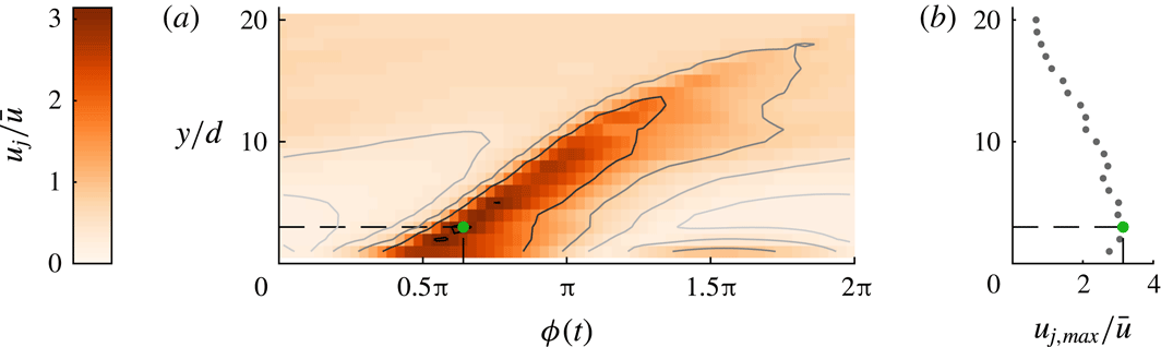
. The phase-averaged centreline velocity of the jet for a single case is presented for different distances to the jet in figure 2. It can be seen that the maximum velocity occurs a small distance away from the orifice exit plane (
 $y=3~\text{mm}$
for this specific case), which can be attributed to the formation of the vortex ring created by the jet (Smith & Glezer Reference Smith and Glezer1998). This true maximum velocity rather than the value at the orifice exit is used to calculate the mean blowing velocity. Figure 2 also indicates the very weak effect of the suction phase which is located at
 $\unicode[STIX]{x1D719}=1.5\unicode[STIX]{x03C0}$
and decays very quickly with distance from the orifice. Under the assumption that the suction phase has a negligible influence on the interaction with a cross-flow, a synthetic jet behaves as a pulsed jet.
(a) Phase-locked jet-centreline velocity over 64 phases as a function of wall-normal distance for case 1 as defined in table 1 (in the absence of cross-flow). (b) Variation of the maximum centreline velocity with wall-normal height. The wall-normal location and phase at which
 $u_{j,max}$
occurs are indicated by the green dot.

2.4 Determining the jet location
Multiple definitions can be used to identify the location of a jet, including positions of local maxima in the velocity deficit, local vorticity maxima or the time-averaged streamline originating from the orifice (Mahesh Reference Mahesh2013). Neither vorticity nor streamlines can be determined from only the velocity magnitude. Identification of local maxima in the velocity deficit requires comparison of a perturbed to an unperturbed case, thereby increasing the uncertainty. Here we consider the location of the jet based on a single dataset by decomposing the velocity signal as
 $$\begin{eqnarray}U(y,t)=\langle U(y)\rangle +\widetilde{U}(y,\unicode[STIX]{x1D719}(t))+U^{\prime }(y,t),\end{eqnarray}$$
where
 $\langle U(y)\rangle$
is the time-averaged local velocity,
 $\widetilde{U}(y,\unicode[STIX]{x1D719}(t))$
is the phase-averaged local velocity at phase
 $\unicode[STIX]{x1D719}(t)$
, and
 $U^{\prime }(y,t)$
are the local velocity fluctuations (similar to Hussain & Reynolds (Reference Hussain and Reynolds1970)); these fluctuations include turbulence as well as fluctuations caused by the interaction of the jet with the cross-flow, which may occur at frequencies other than the jet frequency. A contour map of the phase-averaged component
 $\widetilde{U}$
as a function of phase
 $\unicode[STIX]{x1D719}(t)$
and wall-normal location
 $y^{+}$
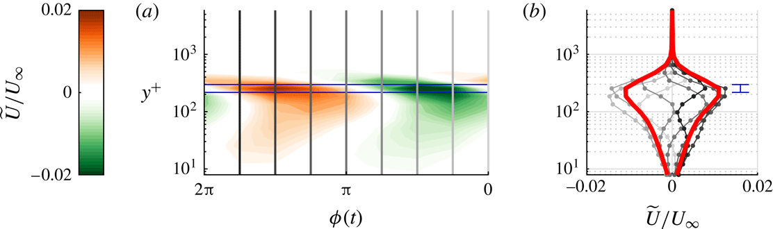
is presented in figure 3(a). A clear maximum of variations in phase can be identified at a wall-normal position indicated by the horizontal blue lines. The velocity at the phases indicated by the vertical lines is presented in figure 3(b), where the root-mean-square (r.m.s.) value is indicated by the thick red lines. The location of the jet is defined as the location where this r.m.s. value reaches its maximum. This location can be determined with an accuracy of one measurement point, leading to an estimated uncertainty on the wall-normal location of the jet of
 $\unicode[STIX]{x1D716}_{y}=0.17y$
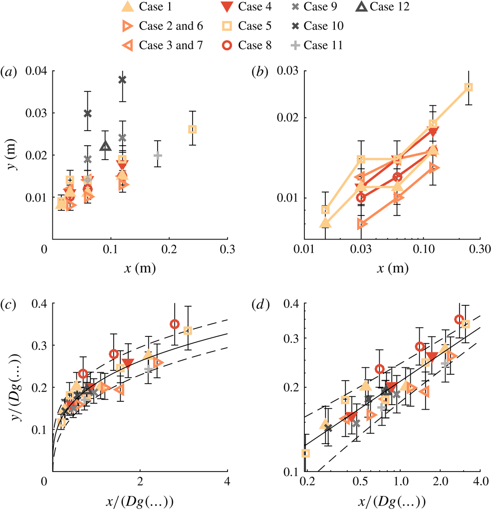
, or 17 %, which is indicated by the blue error bar. This relatively large uncertainty is also displayed in the results in figure 4 and leads to a significant spread in the measurement points. When fitting the results using multiple points, this uncertainty decreases to acceptable levels, as discussed below.
(a) Contour map of the phase-averaged local velocity
 $\widetilde{U}$
with wall-normal distance and phase. (b) Line plot of
 $\widetilde{U}$
where the line grey-scale tint corresponds to the grey-scale tint of the vertical lines in (a). The red lines indicate the r.m.s. over the eight phases; the blue lines indicate the location of the maximum.

(a) Trajectories for all cases listed in table 1. (b) Trajectories of three data points and longer with logarithmic axes indicating a power-law behaviour. (c) Trajectories optimally scaled using the scaling factors in table 2. (d) The same as (c) but with logarithmic axes. Solid lines indicate the fitted trajectory, dashed lines indicate the fit
 $\pm$
the r.m.s. of the residuals. Error bars indicate the error originating from the wall-normal spacing of measurement points as discussed in § 2.4.

3 Results
As discussed above, it is assumed that the trajectory of a synthetic jet issuing into a turbulent boundary layer scales with the Reynolds number (
 $Re_{\unicode[STIX]{x1D70F}}$
), velocity ratio (
 $r$
) and some measure of frequency. The relevant non-dimensional group containing the jet frequency is unknown and could be any of the three groupings listed in (1.8)–(1.10). In an exploratory study, these parameters are varied systematically to determine both the relevant normalization of the frequency as well as the scaling of the trajectory as a function of this determined frequency,
 $Re_{\unicode[STIX]{x1D70F}}$
and
 $r$
. The analysis as presented here is highly dependent on the assumptions made for the important non-dimensional groups. The validity of these assumptions is investigated in appendix A where the same data are fitted against physical parameters first (i.e.
 $g(\ldots )=\bar{u}^{\unicode[STIX]{x1D6FC}_{1}}f^{\unicode[STIX]{x1D6FC}_{2}}D^{\unicode[STIX]{x1D6FC}_{3}}U_{\infty }^{\unicode[STIX]{x1D6FC}_{4}}\unicode[STIX]{x1D6FF}^{\unicode[STIX]{x1D6FC}_{5}}\unicode[STIX]{x1D708}^{\unicode[STIX]{x1D6FC}_{6}}$
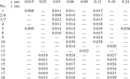
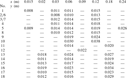
), after which non-dimensional groups are formed using the obtained coefficients. This leads to the same non-dimensional groups as those used in this section, indicating the validity of the assumed important non-dimensional groups. Using the results of the exploratory study, a validation study is performed in which the most important non-dimensional groups are varied systematically. All data points used in this study are provided in appendix B.
Summary of case parameters for the exploratory study. The arbitrary value
 $D=1~\text{m}$
is used to quantify
 $f\,D/U_{\infty }$
.

Fitted coefficients and residuals for
 $y/(Dg(\ldots ))=A(x/(Dg(\ldots )))^{n}$
.

3.1 Exploratory study
Jet and cross-flow parameters are varied systematically as listed in table 1. The first group of cases (1–4) considers a variation in
 $Re_{\unicode[STIX]{x1D70F}}$
while keeping the velocity ratio constant and (roughly) matching the outer-scaled frequency (
 $f\unicode[STIX]{x1D6FF}/U_{\infty }$
) between cases. For the second group (5–8) the Reynolds number is varied for a constant blowing ratio while (roughly) matching the inner-scaled frequency (
 $f\unicode[STIX]{x1D708}/U_{\unicode[STIX]{x1D70F}}^{2}$
). The third group (9–12) considers variations in blowing ratio while matching either inner- or outer-scaled frequencies or matching the blowing ratio and Reynolds number for a variation in frequency (cases 10 and 12). The passing frequency of the jet (
 $f\,D/U_{\infty }$
) is not matched systematically but varied/matched as a result of the others.
For each case, the wall-normal location of the jet is determined at multiple positions downstream of the slot. The measured jet locations are presented in figure 4(a). Error bars indicate the uncertainty in determining the wall-normal location of the jet, which is a result of the wall-normal spacing between measurement points. As expected, the trajectories show some wall-normal variation with especially the cases of higher velocity ratio (9, 10 and 12) standing out. Cases containing three or more points are plotted with logarithmic axes in figure 4(b). The points for each case are on a straight line, indicating that the trajectories follow a power law as hypothesized in § 1. All cases in figure 4(b) have the same slope, which suggest that they can all be described using the same coefficient
 $n$
in (1.6).
The influence of the non-dimensional groups (
 $r$
,
 $Re_{\unicode[STIX]{x1D70F}}$
and
 $f^{\ast }$
) on the trajectory given by (1.6) is quantified by assuming
 $g(\ldots )=r^{c_{1}}Re_{\unicode[STIX]{x1D70F}}^{c_{2}}f^{\ast c_{3}}$
(for
 $f_{1}^{\ast }$
,
 $f_{2}^{\ast }$
and
 $f_{3}^{\ast }$
as defined in (1.8)–(1.10) independently). The coefficients
 $A$
,
 $n$
and
 $c_{1-3}$
are fitted using nonlinear regression. The accuracy of each fit is measured as the r.m.s. of the residuals, i.e.
 $$\begin{eqnarray}\unicode[STIX]{x1D716}=\text{r.m.s.}\;(y-Ax^{n}g(\ldots )^{1-n}).\end{eqnarray}$$
Fitting parameters and accuracy are listed in table 2. Fits are compared to an unscaled power law (
 $g(\ldots )=1$
) and to scaling based on the velocity ratio only as in (1.2) (
 $g(\ldots )=r^{c}$
). Note that the value of
 $A$
depends on the choice of the orifice length scale
 $D$
, which is unknown. For each fit, 28 data points are used, decreasing the estimated uncertainty in the wall-normal location (discussed in § 2.4) to
 $\unicode[STIX]{x1D716}_{y}=0.17y/\sqrt{28}=0.03y$
or 3 %. For a nominal jet height of
 $y=0.02~\text{m}$
, this uncertainty is
 $\unicode[STIX]{x1D716}_{y}\approx 0.6~\text{mm}$
. Comparison of this uncertainty to the residuals of each fit as reported in table 2 suggests that the leading-order uncertainty is in the fitting and not in the measurements.
Based on the residuals, proper normalization of the frequency is as
 $f\,D/U_{\infty }$
(
 $\unicode[STIX]{x1D716}=1.6~\text{mm}$
). The r.m.s. of the residuals using this scaling is almost twice as small as for the velocity-ratio scaling (
 $\unicode[STIX]{x1D716}=2.8~\text{mm}$
) and almost four times as small as for the unscaled case (
 $\unicode[STIX]{x1D716}=5.4~\text{mm}$
). It should be noted that the residuals using the outer-scaled frequency are only slightly higher (20 %) than when using the passing frequency. The difference between these normalizations is caused in this case (where
 $D$
is constant) by
 $\unicode[STIX]{x1D6FF}$
, which is only varied by a factor of 2 for the current experiments, explaining the small difference between the residuals.
The fit using the passing frequency shows a scaling of
 $$\begin{eqnarray}g(\ldots )=r^{1.26}Re_{\unicode[STIX]{x1D70F}}^{-0.04}(f\,D/U_{\infty })^{-0.56}.\end{eqnarray}$$
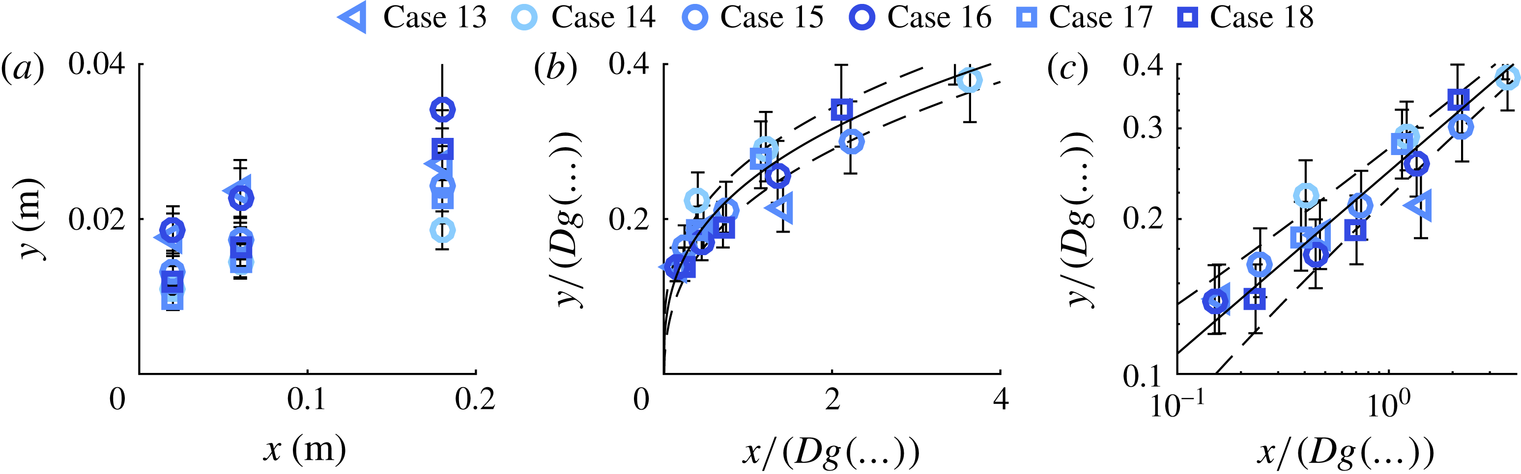
Measured trajectories are scaled using this expression in figure 4(b,c), showing a reasonable collapse for all cases.
This result suggests that (I) the trajectory scales with
 $r^{1.26}$
, which is equal to the scaling for a steady jet, (II) even over the large range of Reynolds numbers tested here (
 $3200<Re_{\unicode[STIX]{x1D70F}}<12\,800$
),
 $Re_{\unicode[STIX]{x1D70F}}$
only has a small effect on the trajectory and (III) scaling of the frequency of the jet is with the passing frequency of the flow over the orifice,
 $f\,D/U_{\infty }$
.
3.2 Validation study
A second experiment is designed as validation of the leading terms (
 $r$
and
 $f\,D/U_{\infty }$
) in (3.2). In this experiment,
 $Re_{\unicode[STIX]{x1D70F}}$
is kept constant while
 $r$
and
 $f\,D/U_{\infty }$
are varied systematically as listed in table 3.


Summary of case parameters for the validation study. The arbitrary value
 $D=1~\text{m}$
is used to quantify
 $f\,D/U_{\infty }$
.

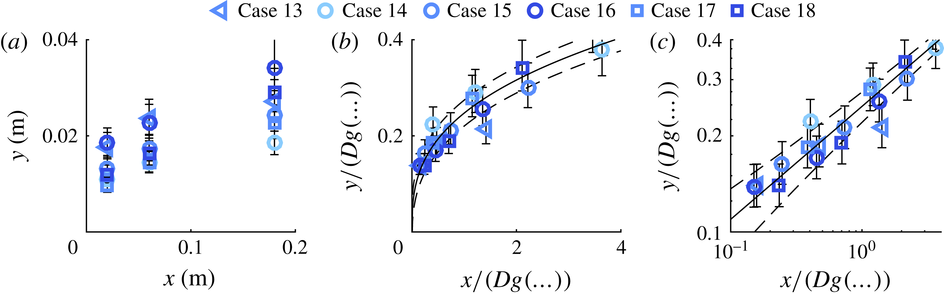
Measured wall-normal locations of the jet for the validation study are presented in figure 5(a). Fitted values for the power law are
 $A=0.27$
and
 $n=0.26$
, which are slightly different from the values for the initial experiment (
 $A=0.26$
,
 $n=0.32$
). Nevertheless, the normalized data in figure 5(b,c) collapse onto a single power law (indicated by the black line), validating the scaling as listed in (3.2).
3.3 Jet decay and very-far-field behaviour
As discussed in § 2.4, the location of the jet is determined using the cyclic velocity perturbations that the jet creates in the cross-flow. These perturbations decay with streamwise distance from the jet exit, and the streamwise extent of the measurements as presented above is limited by this decay. For the most-downstream points of each case, the r.m.s. of the velocity fluctuations has typically decayed down to 0.1 % of the free-stream velocity and the jet could not be detected further downstream.
This same decay implies that, in the very far field, where coherent structures created by the jet have vanished, the fluid ejected by the jet will not penetrate the flow further and the trajectory becomes horizontal. This may suggest a deviation from the power law (which does not become fully horizontal) in the very far field.
4 Discussion
The derived scaling for the trajectory of a synthetic jet issuing into a turbulent boundary layer as stated in (3.2) depends on three non-dimensional groups.
Analogous to steady jets, the trajectory scales with the velocity ratio as
 $y/r^{c}\propto (x/r^{c})^{n}$
. As discussed above, for steady jets usually a value of
 $c=1$
is stated, but in general
 $0<c<2$
. The value found for synthetic jets,
 $c=1.26$
, is well within this range, showing an analogy in the effect of the velocity ratio on trajectories of steady jets and synthetic jets.
For the investigated range of parameters (
 $3200<Re_{\unicode[STIX]{x1D70F}}<12\,800$
), the friction Reynolds number is found to have only a small influence on the trajectory of the jet, scaling as
 $y/Re_{\unicode[STIX]{x1D70F}}^{-0.04}\propto (x/Re_{\unicode[STIX]{x1D70F}}^{-0.04})^{n}$
. This coefficient may be considered to be within experimental uncertainty. Therefore, the trajectory of the jet in the cross-flow is at best weakly dependent on the Reynolds number of the boundary layer and is most likely to be independent of it. This suggests that further studies can be performed in other facilities which do not have the capability of reaching high friction Reynolds numbers. It should be noted that
 $U_{\unicode[STIX]{x1D70F}}$
may have an additional influence on the trajectory, which could not be independently measured due to the dependence of
 $c_{f}$
on
 $Re_{\unicode[STIX]{x1D70F}}$
. The independence of the trajectory on
 $Re_{\unicode[STIX]{x1D70F}}$
does not necessarily imply that the trajectory is equal in laminar boundary layers. Owing to the fuller velocity profile of (high-Reynolds-number) turbulent boundary layers, most of the circulation is concentrated relatively close to the wall compared to laminar boundary layers. As discussed above, this circulation interacts with the vortical structure formed by the jet, leading to geometrically complicated vortical structures. This suggests that turbulent boundary layers have a much larger effect on the created vortical structures and therewith a different effect on the trajectory. It should be noted that the stated independence of Reynolds number is based on high Reynolds numbers (
 $Re_{\unicode[STIX]{x1D70F}}>3200$
) and its scaling is unknown when the laminar limit is approached at low Reynolds numbers. When the boundary-layer thickness is considered independently (see appendix A), it influences the scaling parameter as
 $g(\ldots )\propto \unicode[STIX]{x1D6FF}^{-0.08}$
. While the boundary-layer thickness is varied by a factor of 2.2 in the present study, it only altered the scaling parameter by 6 %. Therefore, other non-dimensional groups containing
 $\unicode[STIX]{x1D6FF}$
(such as
 $\unicode[STIX]{x1D6FF}/D$
) are considered negligible.
It is found that the trajectory scales with the term
 $f\,D/U_{\infty }$
, where
 $D$
is a representative slot dimension added from dimensional arguments. The exact nature of
 $D$
can only be determined by varying the slot dimensions, which was outside the scope of the parametric study in the performed experiments, but it is assumed that
 $D$
is a function of both the slot width
 $d$
and length
 $l$
. The term
 $f\,D/U_{\infty }$
represents a ratio between two length scales, where
 $U_{\infty }/f$
is related to the separation distance between subsequent jet pulses created at time interval
 $1/f$
and with streamwise advection velocity
 $\propto U_{\infty }$
. These length scales are schematically represented in figure 6(a), where it is assumed that the size of jet pulses/vortical structures depends on the representative size of the orifice
 $D$
. As presented in figure 6(b), when increasing this ratio, an interesting phenomenon occurs near unity where the pulses of the jet form a seemingly continuous jet. At the same time, when
 $f\,D/U_{\infty }=1$
(and neglecting the influence of
 $Re_{\unicode[STIX]{x1D70F}}^{-0.04}$
), the scaling factor in (3.2) is given by
 $g(\ldots )=r^{1.26}$
, recovering the scaling for a steady jet (as in (1.2)).
As discussed by Shapiro et al. (Reference Shapiro, King, M’Closkey and Karagozian2006) and Karagozian (Reference Karagozian2014), the waveform used to actuate an unsteady jet has a large influence on the trajectory. Therefore, the results of pulsed and forced jets (often actuated using a square wave) may differ from the results obtained in the present study. However, following the above discussion and the schematic in figure 6, it may be assumed that the obtained scaling holds for unsteady jets that create a train of distinct vortical structures, which (under certain conditions) has been observed for both pulsed jets (e.g. Jabbal & Zhong Reference Jabbal and Zhong2008) and forced jets (e.g. Johari Reference Johari2006).
Schematic indicating the physical meaning of the non-dimensional group
 $f\,D/U_{\infty }$
, which is considered as the ratio between length scales
 $U_{\infty }/f$
, representing the streamwise distance between subsequent pulses of the jet, and
 $D$
, representing the size of these pulses. (a) A case with
 $f\,D/U_{\infty }\ll 1$
and (b) the case
 $f\,D/U_{\infty }=1$
, showing an almost continuous jet.

5 Conclusions
Scaling of the trajectory of a synthetic jet issuing into a turbulent boundary layer is derived. This problem can be described by the slot length
 $l$
and width
 $d$
, the jet frequency
 $f$
and mean blowing velocity
 $\bar{u}$
, the free-stream velocity
 $U_{\infty }$
, the boundary-layer thickness
 $\unicode[STIX]{x1D6FF}$
, the friction velocity
 $U_{\unicode[STIX]{x1D70F}}$
and the kinematic viscosity
 $\unicode[STIX]{x1D708}$
. Six independent non-dimensional groups can be formed out of these parameters. However, owing to the nature of the experiment, the aspect ratio of the jet
 $AR=l/d$
as well as the ratio
 $U_{\infty }/U_{\unicode[STIX]{x1D70F}}$
are fixed, leaving four independent non-dimensional groups to describe scaling of the trajectory of the jet. Fitting of trajectories for a wide parametric study showed that only three independent non-dimensional groups are required to describe these trajectories. The trajectories are shown to scale as
 $$\begin{eqnarray}\frac{y/D}{r^{1.26}Re_{\unicode[STIX]{x1D70F}}^{-0.04}(f\,D/U_{\infty })^{-0.56}}=A\left(\frac{x/D}{r^{1.26}Re_{\unicode[STIX]{x1D70F}}^{-0.04}(f\,D/U_{\infty })^{-0.56}}\right)^{n},\end{eqnarray}$$
where the scaling factors in the denominator are given by the following:
(i)
 $r^{1.26}$
, showing analogy to trajectories of a steady jet in cross-flow which scales with
$r^{c}$
for typical values of
$0<c<2$
.
(ii)
$Re_{\unicode[STIX]{x1D70F}}^{-0.04}$
, indicating only a weak dependence on the friction Reynolds number. This enables future studies in facilities with lower Reynolds numbers.(iii)
$(f\,D/U_{\infty })^{-0.56}$
, where
$D$
is an unknown combination of the slot dimensions
$l$
and
$d$
. This term indicates the relevant non-dimensional number for the jet frequency. This group gives the ratio between two length scales:
$U_{\infty }/f$
, relating to the streamwise spacing between subsequent pulses; and
$D$
, relating to the size of these pulses. It can be argued that when the separation between pulses equals the pulse size, a continuous jet is formed. At the same time, when this ratio goes to unity, the scaling for the trajectory of a steady jet in cross-flow is recovered. These arguments hold for other types of unsteady jets such as pulsed and forced jets. It may be assumed that (under certain conditions) the scaling with frequency is equal for synthetic, pulsed and forced jets. The nature of the relevant orifice dimension
$D$
and the relation to the pulse size as hypothesized above are subjects for further study. Assuming that a single orifice length scale
$D$
exists, results are expected to hold for other orifice shapes when normalized by their respective length scales.


The study was motivated by the application in skin-friction control, which is reflected in the shape of the jet orifice (rectangular with the long dimension aligned with the flow) and the low velocity ratios used in the study. One distinctive aspect of the study is the high Reynolds numbers of the turbulent boundary layers. This is the first study known to the authors to investigate the effect of the friction Reynolds number on the trajectory of a (synthetic) jet in a cross-flow. Furthermore, this is the first study known to the authors to systematically study the effect of the frequency of an unsteady jet on the trajectory.
Acknowledgements
T.B. and B.G. acknowledge the financial support from the European Research Council (ERC grant agreement no. 277472), the Engineering and Physical Sciences Research Council (EPSRC grant no. EP/L006383/1) and Airbus. I.M. and N.H. acknowledge the support of the Australian Research Council.
Appendix A. Fitting of dimensional parameters
Fitting the scaling parameter
 $g(\ldots )$
against pre-assumed non-dimensional groups as in (1.11) limits the result to these assumed groups. The purpose of this appendix is to overcome this limit by fitting the scaling parameter against dimensional parameters. As listed in § 1.5, the parameters describing the interaction of a synthetic jet with a cross-flow are the velocity magnitude
 $\bar{u}$
, frequency
 $f$
and (unknown) orifice length scale
 $D$
of the jet as well as the free-stream velocity
 $U_{\infty }$
, boundary-layer thickness
 $\unicode[STIX]{x1D6FF}$
, friction velocity
 $U_{\unicode[STIX]{x1D70F}}$
and kinematic viscosity
 $\unicode[STIX]{x1D708}$
of the cross-flow. The friction velocity is related to the free-stream velocity through the skin-friction coefficient,
 $c_{f}=2U_{\unicode[STIX]{x1D70F}}^{2}/U_{\infty }^{2}$
, which is a function of
 $\text{log}(Re_{x})$
. For the values of
 $Re_{x}$
used in the present study, the ratio between the friction velocity and free-stream velocity is fairly constant (i.e.
 $U_{\infty }\approx U_{\unicode[STIX]{x1D70F}}\unicode[STIX]{x1D6FD}$
for a constant
 $\unicode[STIX]{x1D6FD}$
). This means that they cannot be fitted independently and
 $U_{\unicode[STIX]{x1D70F}}$
is left out of consideration for the fit. This leads to a description of the trajectory of
 $$\begin{eqnarray}\frac{y}{(\bar{u}^{\unicode[STIX]{x1D6FC}_{1}}f^{\unicode[STIX]{x1D6FC}_{2}}D^{\unicode[STIX]{x1D6FC}_{3}}U_{\infty }^{\unicode[STIX]{x1D6FC}_{4}}\unicode[STIX]{x1D6FF}^{\unicode[STIX]{x1D6FC}_{5}}\unicode[STIX]{x1D708}^{\unicode[STIX]{x1D6FC}_{6}})D}=A\left(\frac{x}{(\bar{u}^{\unicode[STIX]{x1D6FC}_{1}}f^{\unicode[STIX]{x1D6FC}_{2}}D^{\unicode[STIX]{x1D6FC}_{3}}U_{\infty }^{\unicode[STIX]{x1D6FC}_{4}}\unicode[STIX]{x1D6FF}^{\unicode[STIX]{x1D6FC}_{5}}\unicode[STIX]{x1D708}^{\unicode[STIX]{x1D6FC}_{6}})D}\right)^{n}.\end{eqnarray}$$
As discussed in the main text, the orifice length scale
 $D$
is unknown but constant and fitted as
 $D=1~\text{m}$
, which will influence the value of coefficient
 $A$
only. The variation in the viscosity
 $\unicode[STIX]{x1D708}$
throughout the experiments was negligible and
 $\unicode[STIX]{x1D6FC}_{6}$
cannot be reliably fitted by itself. Coefficients
 $\unicode[STIX]{x1D6FC}_{3}$
and
 $\unicode[STIX]{x1D6FC}_{6}$
can then be used for dimensional reasons since the dimensions of the terms within the brackets in the denominator of (A 1) are
 $$\begin{eqnarray}[g(\ldots )]=m^{\unicode[STIX]{x1D6FC}_{1}+\unicode[STIX]{x1D6FC}_{3}+\unicode[STIX]{x1D6FC}_{4}+\unicode[STIX]{x1D6FC}_{5}+2\unicode[STIX]{x1D6FC}_{6}}\hspace{2.22198pt}s^{-\unicode[STIX]{x1D6FC}_{1}-\unicode[STIX]{x1D6FC}_{2}-\unicode[STIX]{x1D6FC}_{4}-\unicode[STIX]{x1D6FC}_{6}}.\end{eqnarray}$$
Given that this term is dimensionless,
 $\unicode[STIX]{x1D6FC}_{3}$
and
 $\unicode[STIX]{x1D6FC}_{6}$
can be determined as
 $$\begin{eqnarray}\displaystyle & \unicode[STIX]{x1D6FC}_{3}=\unicode[STIX]{x1D6FC}_{1}+2\unicode[STIX]{x1D6FC}_{2}+\unicode[STIX]{x1D6FC}_{4}-\unicode[STIX]{x1D6FC}_{5}, & \displaystyle\end{eqnarray}$$
 $$\begin{eqnarray}\displaystyle & \unicode[STIX]{x1D6FC}_{6}=-\unicode[STIX]{x1D6FC}_{1}-\unicode[STIX]{x1D6FC}_{2}-\unicode[STIX]{x1D6FC}_{4}. & \displaystyle\end{eqnarray}$$
The coefficients
 $A$
,
 $n$
and
 $\unicode[STIX]{x1D6FC}_{1-6}$
are fitted against the data presented in § 3.1 using nonlinear regression. Fitted coefficients and the r.m.s. of the residuals (
 $\unicode[STIX]{x1D716}$
) are presented in table 4. In dimensional parameters, the scaling parameter is given by
 $$\begin{eqnarray}g(\ldots )=\bar{u}^{1.22}f^{-0.55}D^{-0.55}U_{\infty }^{-0.75}\unicode[STIX]{x1D6FF}^{-0.08}\unicode[STIX]{x1D708}^{0.08}.\end{eqnarray}$$
Following the Buckingham
 $\unicode[STIX]{x03C0}$
theorem, four independent non-dimensional groups can be formed out of these six dimensional parameters. It should be noted that grouping these parameters can be done in numerous different ways and the chosen groups depend on assumptions.
Fitted coefficients and residuals for (A 1).

Following the literature, it seems sensible to group the jet velocity and cross-flow velocity into a velocity ratio
 $r^{1.22}=(\bar{u}/U_{\infty })^{1.22}$
. From the equal coefficients for the boundary-layer thickness and viscosity, it seems sensible to group these into the friction Reynolds number
 $Re_{\unicode[STIX]{x1D70F}}^{-0.08}=(\unicode[STIX]{x1D6FF}U_{\unicode[STIX]{x1D70F}}/\unicode[STIX]{x1D708})^{-0.08}$
, where the direct relationship between the friction velocity and free-stream velocity is used to substitute
 $U_{\infty }^{0.08}=U_{\unicode[STIX]{x1D70F}}^{0.08}\unicode[STIX]{x1D6FD}^{0.08}$
for
 $\unicode[STIX]{x1D6FD}$
a constant that will alter coefficient
 $A$
. Using these choices, the scaling parameter has reduced to
 $$\begin{eqnarray}g(\ldots )=r^{1.22}Re_{\unicode[STIX]{x1D70F}}^{-0.08}f^{-0.55}D^{-0.55}U_{\infty }^{0.55},\end{eqnarray}$$
which indicates a non-dimensional frequency
 $(f\,D/U_{\infty })^{-0.55}$
. Note that this has led to only three non-dimensional groups where four independent groups were possible. Also note that this analysis has obtained the same non-dimensional groups as the analysis in § 3 with the difference in coefficients being within experimental error.
Using different assumptions, a variety of different groupings are possible. Most notably, the scaling parameter can be represented as
 $$\begin{eqnarray}g(\ldots )=r^{0.67}(L/D)^{0.55}Re_{\unicode[STIX]{x1D70F}}^{-0.08},\end{eqnarray}$$
where
 $L/D$
is the non-dimensional stroke length, which is an important parameter for the formation of vortex rings. This parameter was left out of the assumptions in § 1.5 under the assumption that the scaling of the frequency should include cross-flow parameters. It is included here because it shows some similarity with a theoretical scaling for the trajectory of isolated vortex rings as derived by Johari (Reference Johari2006). This scaling can be represented as
 $$\begin{eqnarray}g(\ldots )=r^{0.33}\left(L/D\right)^{0.33}.\end{eqnarray}$$
Although these expressions take the same form, the coefficients are somewhat different. When this scaling in (A 8) is used to normalize the data (using a best fit for
 $A$
and
 $n$
), a root-mean-square of the residuals of
 $\unicode[STIX]{x1D716}=3.1~\text{mm}$
is obtained. This deviation is larger than when using just velocity-ratio scaling (see table 2), invalidating this scaling for the data in the present study.
Out of all the possible groupings of physical parameters in (A 5), the authors deem the one discussed above and presented in (A 6) most feasible, substantiating the scaling derived in the study.