


1. Introduction
Behavioral bias plays a vital role in shaping household saving behavior, and one’s financial situation can have profound implications for macroeconomic outcomes and policy design (e.g., Farhi and Werning (Reference Farhi and Werning2019), Angeletos and Huo (Reference Angeletos and Huo2021), Pfäuti and Seyrich (Reference Pfäuti and Seyrich2022)). However, this literature generally assumes homogeneous behavioral bias. This assumption contradicts empirical evidence, such as heterogeneity in present bias (e.g., Ameriks et al. Reference Ameriks, Caplin, Leahy and Tyler2007; Chan, Reference Chan2017; Lockwood, Reference Lockwood2020), which affects the model’s predictive power. This evidence raises the following question: Can present bias heterogeneity help us better explain macroeconomic outcomes and guide policy design?
To answer these questions, we incorporate heterogeneous present-biased preferences into the model of Sargent et al. (Reference Sargent, Wang and Yang2021). For tractability, we model present-biased preferences with hyperbolic discount functions in the spirit of Harris and Laibson (Reference Harris and Laibson2013). This formulation captures that agents tend to make decisions using a discount rate that declines in relative time. This feature is in stark contrast to the exponential discount function, where the discount rate remains constant in relative time. Moreover, decision-making is time-inconsistent, so the agent is modeled as a sequence of temporal selves, and the optimal policies can be envisioned as an intrapersonal game between the successive selves. The current selfcontrols the household policies in the current period but derives utility from the entire stream of consumption chosen by her future selves. In our model, the economy is populated by agents with two types of present-biased preferences: completely sophisticated agents who correctly perceive future selves’ present bias and fully naive agents who ignore future selves’ present bias. Individual wealth accumulation is subject to random death shocks, and labor earnings are subject to random income shocks. The agent purchases a “reverse-life-insurance” contract that generates flow payoffs for the living agent in exchange for her terminal wealth upon death shock arrival. Due to market incompleteness, income risk is uninsurable. Access to debt is costly, and heavily indebted households can file for bankruptcy to reduce their leverage. Individuals make the optimal consumption and default choices, and capital market clearing conditions determine the equilibrium interest rate.
We find the following main novel results. First, heterogeneous present bias allows us to match the US average marginal propensity to consume (MPC) while simultaneously matching key statics for wealth distribution in the data. Typically, this is not possible in one-asset HANK models: if the supply of assets is large enough to match the average wealth in the economy, almost all of the households have accumulated a sufficient buffer stock against adverse shocks (Kaplan and Violante, Reference Kaplan and Violante2022). This strong self-insurance effect implies that almost all households should have relatively low MPCs. In our model, however, naive households overlook their future splurging and are overly optimistic about their future financial situations. Consequently, they are more likely to be hand-to-mouth (HtM).Footnote 1 In other words, a large share of naive households are indebted and thus exhibit a high marginal propensity to consume, driving up the average MPC. Sophisticated households, on the other hand, fully understand their future splurging and optimally save more to avoid future financial distress. As a result, wealth inequality in our model is higher than that in its homogeneous preference counterpart and closer to the empirical estimates. Based on our model with heterogenous present bias, we find that consumption is more responsive when fiscal stimulus targets households in the bottom half of wealth distribution.
Second, we explore the welfare implications of a financial literacy campaign that effectively removes present bias. Eliminating present bias disciplines household overconsumption, which improves household welfare in the short run (with fixed interest rates and wealth distribution). Nevertheless, the dark side of the campaign arises when we study its long-run effect. Since present bias reduction encourages aggregate wealth accumulation in the economy, a larger capital supply reduces the equilibrium interest rate in the long run. Naive households with little wealth still benefit from the literacy campaign. Nevertheless, once the household accumulates more wealth, reducing present bias is no longer welfare-improving due to the cost of lower return on wealth accumulation. In a similar vein, for sophisticated households, a lower interest rate is always detrimental because it undermines their wealth accumulation incentives. Our result indicates that the literacy campaign, while potentially beneficial in some circumstances, can also lead to welfare losses, especially for households who stay away from financial distress.
Finally, we investigate the effectiveness of commitment devices such as borrowing cost penalties and illiquidity. They are both double-edged swords. On the cost side, inflexibility undermines consumption smoothing in the short run. On the benefit side, they reduce debt-fueled consumption, thereby disciplining borrowing incentives and improving welfare in the long run. Since they both help curb borrowing incentives, the negative impact of present bias and naivete are partially alleviated.
1.1. Related literature
Two groups of papers relate to this work. Our paper is most related to the research emphasizing the role of consumer heterogeneity in explaining endogenous consumption and wealth inequality. Krusell and Smith (Reference Krusell and Smith1998) find that heterogeneous impatience makes wealthier agents save more and better matches wealth inequality. Similarly, Sargent et al. (Reference Sargent, Wang and Yang2021) incorporate individuals’ survival probability interacted with their heterogeneous preferences about consumption plans to determine aggregate savings and the interest rate. In their model, wealth is more unequally distributed and has a fatter tail than labor earnings, as in US data. Epper et al. (Reference Epper, Fehr, Fehr-Duda, Kreiner, Lassen, Leth-Petersen and Rasmussen2020) combine data from preference-elicitation experiments with high-quality administrative data and provide empirical support for the positive relationship between patience heterogeneity and wealth inequality. Gelman (Reference Gelman2021) provides empirical evidence that transitory circumstances (i.e., cash on hand) and persistent characteristics (i.e., the discount factor) both play important roles in explaining the variance of the MPC. We incorporate heterogeneous degrees of present bias. This model helps match both the aggregate MPC level and the wealth distribution. In addition to the right tail of the wealth distribution, the endogenous wealth distribution aligns with the HtM proportion, median wealth, and mean wealth in the data.
Second, our study is connected to the fast-growing literature exploring hyperbolic discounting in consumption-saving choices (Acharya et al. Reference Acharya, Jimenez Gomez, Rachinskii and Rivera2022; Liu et al. Reference Liu, Niu, Wang and Yang2020; Maxted, Reference Maxted2022). Our model is closely related to Maxted (2022), who characterizes how present bias affects consumption, illiquid asset demand, and welfare. A key departure is that we focus on the impacts of heterogeneous preferences rather than the implications of present bias alone. We show that reducing the present bias of naive households gets them out of the debt trap but incurs negative welfare impacts on sophisticated households due to a lower equilibrium interest rate.
The remainder of the paper proceeds as follows. Section 2 sets up the model. Section 3 derives the solutions for optimal consumption policies. Section 4 presents the stationary distribution with preference heterogeneity. The quantitative results and welfare implications are discussed in Sections 5 and 6, respectively. Finally, we conclude the paper in Section 7.
2. Model setup
We develop a heterogeneous-agent model with uninsurable labor income and ex ante heterogeneity in present-biased preferences. Present bias distorts the intertemporal choices of consumers. Our model aims to explore how heterogeneous present bias affects the wealth distribution and aggregate MPC level.
2.1. Present-biased preferences and utility
2.1.1. Present bias
Suppose that the agent is risk averse and displays present bias in the form of quasi-hyperbolic discounting (Harris and Laibson, Reference Harris and Laibson2013). Time is divided into two periods: the current and the future. The agent exponentially discounts consumption flows in the current period with a discount rate
 $\rho \gt 0$
and further discounts future consumption flows with an additional discount factor
 $\beta \in (0,1)$
, which undermines the present value of consumption flows in future periods.
We model the agent as a sequence of temporal selves. Self
 $1$
is born at time
 $t_1$
. She regards
 $[t_{1},t_2)$
as the current period and treats
 $[t_{2},\infty )$
as the future periods, and in the current period, she controls the consumption-saving decisions. At time
 $t_2$
, self
 $2$
replaces self
 $1$
. She takes control of the consumption-saving choices in the new current period
 $[t_2,t_{3})$
and treats
 $[t_{3},\infty )$
as the new future periods. Thus,
 $T_n=t_{n+1}-t_n$
is the lifespan for self
 $n$
. Assume that the lifespan of each self is exponentially distributed with the constant parameter
 $\xi \gt 0$
. That is, the transition of selves is regulated by a Poisson process with a hazard rate
 $\xi$
. Repeating the process, we can obtain a sequence of selves
 $n\in \{1,2,\ldots \}$
. They live in a sequence of time intervals
 $\{[t_1,t_{2}),[t_2,t_{3}),\ldots \}$
, which are independent and identically distributed (i.i.d.).
Denote by
 $D_n(t,u)$
the quasi-hyperbolic discount function for self
 $n$
; thus, we have:
 \begin{eqnarray} D_n(t,u)=\left \{ \begin{array}{l@{\quad}c} e^{-\rho (u-t)}, &{\textit{if }\ u\in [t_n,t_{n+1})}\\ \beta e^{-\rho (u-t)}, &{\textit{if }\ u\in [t_{n+1},\infty )} \end{array} \right . \end{eqnarray}
where
 $u\gt t$
and
 $t_n\lt t_{n+1}$
. For tractability, we focus on the limiting case when
 $\xi \rightarrow \infty$
, known as the instantaneous gratification (IG) model pioneered by Harris and Laibson (Reference Harris and Laibson2013). In this case, the above discount function (1) becomes:
 \begin{eqnarray} D(t,u)=\left \{ \begin{array}{l@{\quad}c} 1, &{\textit{if }\ u=t}\\ \beta e^{-\rho (u-t)}, &{\textit{if }\ u\gt t} \end{array} \right . \end{eqnarray}
A higher magnitude of present bias is measured by a smaller
 $\beta$
. If
 $\beta =1$
, equation (2) reduces to the traditional exponential discount function.
Models related to present bias require an assumption about the extent to which agents are aware of their future self-control problems (O’Donoghue and Rabin, Reference O’Donoghue and Rabin1999, Reference O’Donoghue and Rabin2001). In this paper, we focus on two types of present-biased agents: (i) completely sophisticated agents, where the current self correctly perceives her future selves’ present bias (Laibson, Reference Laibson1997), and (ii) fully naive agents, where the current self (falsely) believes that her future selves will act in a time-consistent manner (Akerlof, Reference Akerlof1991).
2.1.2. Utility
Suppose that an agent is born at age
 $0$
and dies at a random nonnegative age
 $\tau$
that is exponentially distributed with a constant mortality hazard rate
 $\lambda$
. Across agents, random deaths are statistically independent. To sustain a constant population, we assume that the newborn arrives at a constant rate
 $\lambda$
per unit of time. The agent accrues constant relative risk aversion utility over positive consumption flows
 $\{C_t\}_{t=0}^\tau$
:
 \begin{eqnarray} U(C)= \frac{C^{1-\gamma }}{1-\gamma },\quad{\gamma \gt 0\text{ and }\gamma \neq 1}, \end{eqnarray}
where
 $\gamma$
denotes the coefficient of relative risk aversion.
2.2. Labor income and household borrowing
In this section, we introduce two interrelated “regimes.” In a “normal” regime, the household decides her optimal consumption strategy and services her debt obligations. Once the household defaults on existing debt, she enters a “default” regime from which she cannot leave.
2.2.1. Normal regime
We model the labor income in the normal regime,
 $Y_t$
, as a diffusion process. All agents start life with identical labor earnings
 $Y_0\gt 0$
. The law of motion for labor income is given by:
 \begin{eqnarray} dY_t=\mu Y_tdt+\sigma Y_td\mathcal{B}_t,\quad Y_0\gt 0, \end{eqnarray}
where
 $\mathcal{B}_t$
is a standard Brownian motion,
 $\mu$
is an expected earnings growth rate, and
 $\sigma$
is a volatility of earnings.
Let
 $X_t$
be an agent’s wealth at time
 $t$
, and the initial wealth for all agents is equal to zero, that is,
 $X_0=0$
. With liquid wealth
 $X_t\gt 0$
, the agent can trade a risk-free financial asset that offers a constant risk-free rate of return
 $r$
and purchase an actuarially fair “reverse-life-insurance” contract that transfers end-of-life wealth
 $X_{\tau ^-}$
at time
 $\tau$
to an insurance company in exchange for flow payoffs
 $\lambda X_t\gt 0$
until death. Conversely,
 $X_t\lt 0$
implies that the agent borrows on a credit card, she can transfer end-of-life debt to an insurance company by paying flow expenditures
 $\lambda X_t\lt 0$
; in addition, the agent should pay a borrowing wedge of
 $w^{r}\gt 0$
over the sum of the risk-free rate and the mortality hazard rate
 $r+\lambda$
. Accordingly, the wealth process is given by:
 \begin{eqnarray} dX_t=&\underbrace{\left [(r+\lambda +w^{r}\unicode{x1D7D9}_{\{X_{t-}\lt 0\}}) X_{t-}+Y_{t-}-C_{t-}\right ]}_{\text{saving rate, }G_{t-}}dt -X_{t-}d\mathcal{J}_t, \end{eqnarray}
where
 $\mathcal{J}$
is a pure jump process with a constant arrival rate of
 $\lambda$
and
 $\unicode{x1D7D9}_{\{X_{t-}\lt 0\}}$
is an indicator function that equals one when
 $X_{t-}\lt 0$
, zero otherwise. On the right-hand side of (5), the first term represents the saving rates
 $G_{t-}$
, and the second term captures a one-time transfer
 $X_{\tau ^-}$
from the agent to the insurance company at the stochastic death moment
 $\tau$
when
 $d\mathcal{J}_{\tau }=1$
.
2.2.2. Default regime
Suppose that an agent’s labor income deteriorates sufficiently due to an economic downturn. In that case, the agent reneges on her debt and is henceforth shunned from credit markets, forcing her savings (and debts) to equal zero. This feature reflects that a majority of households go through bankruptcy file Chapter 7 — in which case debtors forfeit nonexempt assets in exchange for a discharge of eligible debts (Dobbie and Song, Reference Dobbie and Song2015).
Let
 $\tau _d$
denote the default arrival time and
 $\widehat Y_t$
denote the labor income in the default regime. Following Bos et al. (Reference Bos, Breza and Liberman2018), we assume that at time
 $\tau _d$
, the labor income immediately drops from
 $Y_{\tau _d-}=\lim _{u\uparrow \tau _d-}Y_u$
, the pre-default income level, to
 $\widehat Y_{\tau _d}=\kappa Y_{\tau _d-}$
, where the constant
 $(1-\kappa )\in (0,1)$
measures the degree of income loss incurred by default, and then the agent permanently enters a default regime. In this regime, the agent can no longer borrow or save
 $(X_t=0)$
, and the earnings
 $\widehat Y_t$
follow the same process (4) as earnings in the normal regime:
 \begin{eqnarray} d\widehat Y_t=\mu \widehat Y_tdt+\sigma \widehat Y_td\mathcal{B}_t. \end{eqnarray}
This process starts at time
 $\tau _d$
with the value of
 $\widehat Y_{\tau _d}=\kappa Y_{\tau _d-}$
.
3. Consumption-saving choice: Intrapersonal game
Under IG time preferences, each self faces self-control problems and disagrees with the expected consumption decisions of future selves. Hence, our consumption-saving problem is a dynamic intrapersonal game played by different selves of the same consumer (Strotz, Reference Strotz1955; Laibson, Reference Laibson1997). Following Harris and Laibson (Reference Harris and Laibson2013), we use a stationary Markov perfect equilibrium (MPE) as the solution concept for the intrapersonal game (Maskin and Tirole, Reference Maskin and Tirole2001). By doing so, a crucial property of IG preferences is that the intrapersonal equilibrium is unique and can be characterized by solving the model without present bias (Harris and Laibson, Reference Harris and Laibson2013; Maxted, Reference Maxted2022).
3.1. Normal regime
3.1.1. Valuation
Under sophisticated IG preferences, the agent correctly anticipates her future selves’ self-control problems. In this situation, the actual continuation-value function is given by:
 \begin{eqnarray} F^S(X_t,Y_t)=\mathbb{E}_t\left [\int ^{\tau \wedge \tau ^S_d}_0 e^{-\rho (u-t)}U\left (C^S_u\right )du\right ], \end{eqnarray}
where
 $C^S_t$
and
 $\tau ^S_d$
denote the consumption rate and default policy adopted by the sophisticated agent, respectively. Then, the actual current-value function is equal to:
 \begin{eqnarray} V^S(X_t,Y_t)=\beta F^S(X_t,Y_t). \end{eqnarray}
The intuition for equation (8) is as follows. The current self discounts the utility of all future selves by
 $\beta$
. Nevertheless, in continuous time, the current self lives only for a vanishingly short time interval (
 $\xi \rightarrow \infty$
); thus, the utility received by the current self has no measurable impact on the overall value function.
Under naive IG preferences, the household (incorrectly) believes that her future selves will behave according to standard exponential discounting. In this situation, the naive agent’s perceived continuation-value function satisfies:
 \begin{eqnarray} F^E(X_t,Y_t)=\mathbb{E}_t\left [\int ^{\tau \wedge \tau ^E_d}_0 e^{-\rho (u-t)}U\left (C^E_u\right )du\right ], \end{eqnarray}
where
 $C^E_t$
and
 $\tau ^E_d$
denote the consumption rate and default strategy adopted by the exponential agent, respectively. The perceived current-value function is
 \begin{eqnarray} V^E(X_t,Y_t)=\beta F^E(X_t,Y_t). \end{eqnarray}
Define
 $F^N(X,Y)$
and
 $C^N(X,Y)$
as the naive agent’s actual continuation-value function and consumption policy, respectively. Next, we show how to derive the optimal consumption policies in the presence of IG preferences.
3.1.2. Optimal consumption rules
Under a stationary MPE, the Bellman equation for the type-
 $j$
agent is given by:
 \begin{eqnarray} \begin{split} (\rho +\lambda )F^j(X,Y)=& \underbrace{U(C^j)}_{\text{utility}} +\underbrace{G^j(X,Y){F^j_X(X,Y)}}_{\text{evolution of }dX} \\[5pt]&+\underbrace{\mu Y{F^j_Y(X,Y)}+\frac{\sigma ^2}{2}Y^2{F^j_{YY}(X,Y)}}_{\text{evolution of }dY},\quad j\in \{S,N\}, \end{split} \end{eqnarray}
which shows that the instantaneous change in value due to discounting and mortality risk,
 $ (\rho +\lambda )F^j(X,Y)$
, must equal the current utility flow,
 $U(C^j)$
, plus the expected instantaneous change in the value function,
 $\left (\mathbb{E}\left (dF^j\right )/dt\right )$
.
The consumption optimality conditions under sophistication and naivete are given by, respectively:
 \begin{eqnarray} U^{\prime}(C^S)=\beta F^S_X(X,Y),\quad U^{\prime}(C^N)=\beta F^E_X(X,Y), \end{eqnarray}
where the marginal utility of consumption on the left-hand side,
 $U^{\prime}(C^S)$
or
 $U^{\prime}(C^N)$
, equals the marginal value of current liquid wealth on the right-hand side,
 $\beta F^S_X(X,Y)$
or
 $\beta F^E_X(X,Y)$
.
Two observations can be drawn from equation (12). First, present bias alters the consumption optimality condition by a multiplicative factor of
 $\beta$
. To see this, note that a standard exponential agent would determine consumption according to:Footnote 2
 \begin{eqnarray} U^{\prime}(C^E)=F^E_X(X,Y). \end{eqnarray}
Evidently, under IG preferences, the marginal value of current liquid wealth is discounted by
 $\beta$
, which arises because wealth is consumed by future selves whose utility is discounted by
 $\beta$
. Second, the optimality condition under sophistication uses the value function of the present-biased agent
 $F^S(X,Y)$
. In contrast, the condition under naivete uses the value function of the exponential-discounting agent
 $F^E(X,F)$
. This difference reflects the naive agent’s (incorrect) belief.
3.2. Default regime
In the default regime, wealth (or debt) is zero, and the household can neither borrow nor save. Hence, consumption equals labor income, and wealth is not an argument of the value function. Under this circumstance, behavioral bias cannot affect consumption rules, and thus, all agents behave as exponential discounters, whose value function is denoted by
 $\widehat F^E(\widehat Y)$
. This function satisfies the following differential equation:
 \begin{eqnarray} \begin{split} (\rho +\lambda ){\widehat F^E(\widehat Y)}=U(\widehat C^E)+\mu \widehat Y\widehat F^{E^{\prime}}(\widehat Y) +\frac{\sigma ^2}{2}\widehat Y^2\widehat F^{E^{\prime\prime}}(\widehat Y), \end{split} \end{eqnarray}
where
 $\widehat C^E=\widehat Y$
. The first term on the right-hand side of (14) gives the utility received by the household in the default regime. The second and third terms capture the impact of drift and volatility of income on the household’s value function
 $\widehat F^E(\widehat Y)$
, respectively.
3.2.1. Debt capacity
 $\underline{X}_t$

In the two regimes, the value functions
 $F^j(X,Y)$
and
 $\widehat F^E(\widehat Y)$
are connected by the transition from the normal to the default regime. To see this, note that upon default, the labor earnings decrease from
 $Y_{t-}$
to
 $Y_t=\kappa Y_{t-}$
, and the wealth jumps from
 $X_{t-}\lt 0$
to
 $X_t=0$
. As a result, the value of wealth at the default time, which we denote by
 $\underline{X}_t$
and makes the household indifferent between repaying her debt and defaulting, satisfies the following value-matching condition:
 \begin{eqnarray} F^j(\underline{X}_t,Y_t)=\widehat F^E(\kappa Y_t),\quad j\in \{S,N\}. \end{eqnarray}
We refer to
 $\underline{X}_t$
as the household’s debt capacity since it is the maximum amount of debt the household can borrow without triggering default in equilibrium. For tractability, we assume that when the household’s income is less than the interest payments to debt, that is,
 $Y_t\lt -(r+\lambda +w^r)X_t$
, the household defaults. Therefore, the debt capacity
 $\underline{X}_t$
is a function of
 $Y_t$
and equals:
 \begin{eqnarray} \underline{X}_t=-\frac{Y_t}{r+\lambda +w^r}. \end{eqnarray}
3.3. Exploiting the homogeneity property
To solve the Bellman equation (11), a key step in our derivation is to establish that the value function in the normal regime,
 $F^j(X,Y)$
, takes the following form:
 \begin{eqnarray} F^j(X,Y)=\frac{\left (b^jP^j(X,Y)\right )^{1-\gamma }}{1-\gamma },\quad j\in \{S,N\}, \end{eqnarray}
where the constant
 $b^j$
is defined in Appendix A. The function
 $P^j(X,Y)$
is interpreted as the certainty-equivalent wealth (CEW), which is the total wealth that makes the household indifferent between the status quo (with liquid wealth
 $X$
and labor income
 $Y$
) and having a wealth level
 $P(X,Y)$
with no labor earnings:
 \begin{eqnarray} F^j(X,Y)=F^j(P^j(X,Y),0). \end{eqnarray}
Similarly, we show that the value function in the default regime,
 $\widehat F^E(\widehat Y)$
, is given by:
 \begin{eqnarray} \widehat F^E(\widehat Y)=\frac{\left (b^E\widehat P^E(\widehat Y)\right )^{1-\gamma }}{1-\gamma }, \end{eqnarray}
where the constant
 $b^E$
is given in Appendix A and
 $\widehat P^E(\widehat Y)$
is the CEW in the default regime. By linking the agent’s value function to her CEW, we can transform the agent’s payoff from the value function to the CEW.
Applying the homogeneity property, we can analyze the (scaled) CEW
 $p^j(x)=P^j(X,Y)/Y$
and the consumption-income ratio
 $c^j(x)=C^j(X,Y)/Y$
in terms of a single state variable,
 $x=X/Y$
, which denotes the wealth-income ratio. Equation (16) shows that the (scaled) debt capacity
 $\underline{x}=\underline{X}/Y=-1/(r+\lambda +w^r)$
is a constant and independent of the present bias parameter
 $\beta$
. By using Ito’s lemma, the law of motion for the wealth-income ratio process is given by:
 \begin{eqnarray} dx^j_t=\underbrace{\left [1+\left (r+\lambda +w^{r}\unicode{x1D7D9}_{\left \{x^j_{t-}\lt 0\right \}} -\mu +\sigma ^2\right )x^j_{t-}-c^j_{t-}\right ]}_{\text{saving rate, }g^j_{t-}}dt -\sigma x^j_{t-}d\mathcal{B}_t -x^j_{t-}d\mathcal{J}_t. \end{eqnarray}
The following proposition summarizes the main results in this section.
Proposition 1. (Present bias and overconsumption) The optimal consumption rules for sophisticated and naive agents are given by, respectively:
 \begin{eqnarray} c^S(x)=\frac{\gamma }{\gamma +\beta -1}c^E(x),\quad c^N(x)={\beta }^{-\frac{1}{\gamma }}c^E(x), \end{eqnarray}
where
 $c^{E}(x)=\left (b^E\right )^{1-1/\gamma }p^{E}(x)\left (p^{E^{\prime}}(x)\right )^{-1/\gamma }$
denotes the consumption-income ratio adopted by the exponential-discounting agent and the scaled CEW
 $p^E(x)$
in the normal regime (
 $x\geq \underline{x}$
) solves the following ordinary differential equation (ODE):
 \begin{eqnarray} \begin{split} 0=&\left [\frac{\gamma \left (b^Ep^{E^{\prime}}(x)\right )^{1-1/\gamma }-(\rho +\lambda )}{1-\gamma }+\mu -\frac{\gamma \sigma ^2}{2}\right ]p^E(x) +p^{E^{\prime}}(x) \\&+\left (r+\lambda +w^{r}\unicode{x1D7D9}_{\{x\lt 0\}}-\mu +\gamma \sigma ^2\right )xp^{E^{\prime}}(x) +\frac{\sigma ^2x^2}{2}\left [p^{E^{\prime\prime}}(x)-\gamma \frac{\left (p^{E^{\prime}}(x)\right )^2}{p^{E}(x)}\right ]. \end{split} \end{eqnarray}
The boundary conditions for (22) are
 \begin{eqnarray} p^E(\underline{x})=\kappa \hat p^E, \lim _{x\rightarrow \infty }p^{E}(x)=x+q, \end{eqnarray}
where the constant
 $q={1}/\left ({r+\lambda -\mu }\right )$
and the scaled value in the default regime,
 $\hat p^E=\widehat P^E(\widehat Y)/\widehat Y$
, is:
 \begin{eqnarray} \hat p^E=\left (b^E\right )^{-1}\left [\rho +\lambda -(1-\gamma ) \left (\mu -\frac{\gamma \sigma ^2}{2}\right )\right ]^{\frac{1}{\gamma -1}}. \end{eqnarray}
To ensure that
 $\hat p^E$
is nonnegative, we impose the following condition:
 \begin{eqnarray} \rho +\lambda -(1-\gamma ) \left (\mu -\frac{\gamma \sigma ^2}{2}\right )\gt 0. \end{eqnarray}
Proof. All proofs are presented in Appendix A.
The economic interpretation of Proposition1 is as follows. First, equation (21) implies that relative to the exponential-discounting agent, sophistication (naivete) induces overconsumption by a multiplicative factor of
 $\frac{\gamma }{\gamma +\beta -1}\gt 1$
(
 ${\beta }^{-\frac{1}{\gamma }}\gt 1$
), since
 $\beta \in (0,1)$
. This result is intuitive: Under IG preferences, the desire for instantaneous gratification drives the agent to overconsume. Second, the first condition in equation (23) follows from the value-matching condition (15) at the default threshold. The second condition implies that when the wealth
 $X$
approaches infinity, the CEW
 $\lim _{X\rightarrow \infty }P^E(X,Y)=X+qY$
is simply the sum of wealth
 $X$
and the “human” wealth
 $qY$
, which is proportional to contemporaneous income. This is because the agent can use holdings of the single risk-free asset completely to buffer all idiosyncratic labor-earning shocks.
4. Ex ante preference heterogeneity
A central result in this section regards how ex ante preference heterogeneity alters the equilibrium wealth distribution. To this end, we assume that the economy is populated by naive and sophisticated agents. These two groups of agents differ not only in their awareness of future present bias but also in the degree of present bias. We assume that naive agents are more present-biased than their sophisticated counterparts, that is,
 $0\lt \beta ^N\lt \beta ^S\lt 1$
. Let
 $\eta ^N$
denote the proportion of naive agents and
 $\eta ^S$
denote the proportion of sophisticated agents, where
 $\eta ^N+\eta ^S=1$
.
4.1. Stationary distribution
4.1.1. Stationary probability density function
Let
 $X^j_t$
and
 $Y^j_t$
denote the type-
 $j$
agent’s wealth and labor earnings at time
 $t$
, respectively. To calculate the cross-sectional stationary probability density of labor earnings
 $\phi ^j_{Y}(Y)$
and wealth
 $\phi ^j_{X}(X)$
, we start by solving the cross-sectional joint distribution of wealth and labor earnings
 $\phi ^j_{XY}(X,Y)$
. After obtaining
 $\phi ^j_{XY}(X,Y)$
, we can compute the cross-sectional stationary distributions of wealth and income by integrating over
 $Y$
and
 $X$
, respectively:
 \begin{eqnarray} \phi ^j_X(X)=\int _0^{+\infty }\phi ^j_{XY}(X,Y)dY,\quad \phi ^j_Y(Y)=\int _{-\infty }^{+\infty }\phi ^j_{XY}(X,Y)dX. \end{eqnarray}
Define
 $X_t$
and
 $Y_t$
as the aggregate wealth and labor income in the economy, respectively. After obtaining the probability density function for each group, we can compute the expectation of aggregate wealth
 $\mathbb{E}(X)$
and aggregate earnings
 $\mathbb{E}(Y)$
according to:
 \begin{eqnarray} \mathbb{E}(X)=\sum _{j=\{N,S\}}\eta ^j\mathbb{E}(X^j),\quad \mathbb{E}(Y)=\sum _{j=\{N,S\}}\eta ^j\mathbb{E}(Y^j), \end{eqnarray}
where
 $\mathbb{E}(X^j)=\int _{-\infty }^{+\infty } X\phi ^j_X(X)dX$
and
 $\mathbb{E}(Y^j)=\int _{0}^{+\infty } Y\phi ^j_Y(Y)dY$
are the average wealth and income for type-
 $j$
group of agents, respectively.
4.1.2. Simulation of stationary distribution
We compute the cross-sectional equilibrium wealth and income distribution by simulation. Specifically, we start by simulating a path of the standard Brownian motion
 $\mathcal{B}_t$
with
 $\mathcal{B}_0=0$
. Next, we use the process for
 $x^j_t$
given in (20) together with the optimal consumption-income ratio
 $c^j(x_t)$
given in (21) to obtain the path for the agents’ wealth-income ratio
 $x^j_t$
with
 $x^j_0=X_0/Y_0=0$
. Once
 $x^j_t$
is less than the debt capacity
 $\underline{x}$
, this agent immediately enters the default regime, and her debt becomes zero, which implies that her wealth-income ratio equals zero forever until she dies. Then, we substitute the simulated path of
 $\mathcal{B}_t$
into the process for labor earnings given in (4) with the initial value
 $Y_0$
and then derive the corresponding simulated path for
 $Y^j_t$
. If the agent defaults during her life, the income drops from
 $Y^j_{t-}$
to
 $Y^j_t=\kappa Y^j_{t-}$
, and we use the process given in (6) to generate the path for labor earnings in the default regime. Finally, we derive the wealth
 $X^j_t$
by multiplying the two paths
 $x^j_t$
and
 $Y^j_t$
at each
 $t$
. When an agent dies, we bring in a new agent with zero wealth and
 $Y_0$
. We continue this process until we reach a very high number of years. In this economy, the proportion of naive to sophisticated households is fixed at
 $\eta ^N/\eta ^S$
.
4.1.3. Wealth inequality
To numerically illustrate the impacts of preference heterogeneity on wealth inequality, we introduce two widely used measures of inequality. First, the Lorenz curve of wealth
 $\mathcal{L}_X(z)$
measures the proportion of aggregate wealth captured by the bottom
 $z$
percent of people, which is given by:
 \begin{eqnarray} \mathcal{L}_X(z)=\frac{\int _{0}^z\Phi _X^{-1}(z)dz}{\int _0^1\Phi _X^{-1}(z)dz}, \end{eqnarray}
where
 $\Phi _X^{-1}({\cdot})$
is the inverse of the cumulative distribution function (CDF),
 $\Phi _X({\cdot})$
. Second, previous literature also applies the Gini coefficient to measure the magnitude of wealth inequality, which equals:
 \begin{eqnarray} \Gamma _X=2\int _0^1(z-\mathcal{L}_X(z))dz. \end{eqnarray}
4.2. Equilibrium interest rate
Assume that a representative firm operates a production function
 $F(K,L)=AK^\alpha L^{1-\alpha }$
, where
 $\alpha \in (0,1)$
,
 $A\gt 0$
represents productivity,
 $K$
denotes the aggregate capital stock that depreciates at a constant rate
 $\delta \gt 0$
, and
 $L$
is the aggregate labor stock. The firm rents capital and labor in competitive markets. In the stationary equilibrium, capital demand equals capital supply:
 \begin{eqnarray} K=\mathbb{E}(X). \end{eqnarray}
Suppose each agent inelastically supplies
 $H\gt 0$
h of labor. In equilibrium, labor demand equals labor supply
 $L=H$
. Define
 $w=\mathbb{E}(Y)/H$
as an average wage rate across all agents. Since aggregate labor cost
 $wL$
equals aggregate labor earnings
 $wH$
, the law of large numbers implies
 \begin{eqnarray} wL=wH=\mathbb{E}(Y). \end{eqnarray}
Now, the steady-state equilibrium interest rate
 $r$
can be stated as follows.
Proposition 2. (Equilibrium interest rate with preference heterogeneity). In a competitive equilibrium, the firm’s optimization problem indicates that the equilibrium interest rate
 $r$
is given by:
 \begin{eqnarray} r &=& F_K(K,L)-\delta = A\alpha \left (\frac{K}{L}\right )^{\alpha -1}-\delta = \frac{\alpha }{1-\alpha }\frac{wH}{K}-\delta = \frac{\alpha }{1-\alpha }\frac{\mathbb{E}(Y)}{\mathbb{E}(X)}-\delta, \end{eqnarray}
where the third equality follows from the expression for the equilibrium average wage rate:
 \begin{eqnarray} w &=& F_L(K,L)=A(1-\alpha )\left (\frac{K}{L}\right )^\alpha = A(1-\alpha )\left (\frac{\mathbb{E}(X)}{H}\right )^\alpha . \end{eqnarray}
Given the interest rate
 $r$
, the equilibrium wage rate
 $w$
, initial labor earnings
 $Y_0$
, and aggregate capital
 $K$
are jointly determined by equations (31) through (33).Footnote 3
Proposition3 shows that a higher expected wealth
 $\mathbb{E}(X)$
incurs a lower equilibrium interest rate. To understand this result, note that the equilibrium interest rate is determined by the representative firm’s demand for capital and household savings. A higher
 $\mathbb{E}(X)$
implies that household saving increases, thus raising the capital supply. To strengthen the firm’s demand for capital and clear the asset market, the equilibrium interest rate
 $r$
must decrease. By contrast, a higher expected labor income
 $\mathbb{E}(Y)$
leads to a higher equilibrium interest rate. This is because a higher
 $\mathbb{E}(Y)$
strengthens the agent’s incentive to consume; thus, the representative firm will demand more capital for production. As a result, the equilibrium interest rate increases to encourage savings.
5. Quantitative results
This section analyzes the main results. Section 5.1 describes the parameter values used in our model. Section 5.2 characterizes the properties of optimal consumption-saving rules in the presence of present bias. Section 5.3 analyzes the impacts of present-biased preferences on the average MPC and wealth distribution. Finally, we study the efficiency of wealth targeted stimulus payments in Section 5.4.
5.1 Calibration
First, we follow Prescott (Reference Prescott1986) and Cooley and Prescott (Reference Cooley and Prescott1995) and set the capital share of income
 $\alpha$
to 0.36. We set an annual depreciation rate of
 $\delta$
to
 $1.6\%$
to match an aggregate capital-output ratio
 $K/F(K,L)$
to
 $4.5$
as reported in Piketty (Reference Piketty2014). We set the productivity parameter
 $A$
to
 $0.774$
, so that the wage rate
 $w$
for an agent with the average labor efficiency equals unity. We set the coefficient of risk aversion
 $\gamma$
to
 $1.5$
, as in Attanasio et al. (Reference Attanasio, Banks, Meghir and Weber1999) and Gourinchas and Parker (Reference Gourinchas and Parker2002). Following Castañeda, Díaz-Giménez, and Ríos- Rull (Reference Castañeda, Díaz-Giménez and Ríos-Rull2003), we set the hazard parameter
 $\lambda =0.0167$
to target an agent’s expected lifetime at
 $1/\lambda =60$
years. We assume that the present bias parameter
 $\beta$
ranges from
 $0.5$
to
 $1$
. This is consistent with the literature, such as Laibson (Reference Laibson1997), Harris and Laibson (Reference Harris and Laibson2013), and Laibson et al. (Reference Laibson, Lee, Maxted, Repetto and Tobacman2024).
Second, we calibrate the expected income growth
 $\mu$
and labor earnings growth volatility
 $\sigma$
by targeting a pair of quantities: a mean labor income of
 $\$106,250$
(see 2019 Survey of Consumer Finances, SCFFootnote 4) and a Gini coefficient for the cross-sectional labor earnings of
 $0.63$
(Castañeda, Díaz–Giménez, and Ríos– Rull, Reference Castañeda, Díaz-Giménez and Ríos-Rull2003). Similarly, De Nardi (Reference De Nardi2004) targets the Gini coefficient of labor earnings by calibrating income growth volatility. The calibrated values are
 $\mu =1.28\%$
and
 $\sigma =9.76\%$
. These values are also in line with estimates reported by Meghir and Pistaferri (Reference Meghir and Pistaferri2011).
Finally, we want an average equilibrium wealth of
 $\$746,820$
as in the 2019 SCF, which in light of equation (32) leads to an equilibrium interest rate
 $r$
equals
 $6.4\%$
per annum. With respect to household borrowing and default, we set the borrowing wedge
 $w^r$
to
 $12.46\%$
and the income loss parameter
 $\kappa$
to
 $0.3$
.
5.2 Optimal consumption policies and present bias
Effects of present bias on consumption-saving rules. This picture depicts the optimal consumption and saving rules. Solid blue lines represent the exponential-discounting case, red dashed lines represent the sophisticated case (
 $\beta ^S=0.783$
), and yellow dotted lines represent the naive case (
 $\beta ^N=0.783$
). Under naive (sophisticated) beliefs, the steady-state wealth-income ratio is
 $\tilde x^N=-0.085$
(
 $\tilde x^S=-0.071$
). Other parameter values are reported in Table 1.

First, Panel A of Figure 1 plots the optimal consumption-income ratio against the wealth-income ratio
 $x$
.Footnote 5 When the credit limit is distant (i.e.,
 $x\geq 0$
), the consumption-income ratio
 $c(x)$
is increasing and concave in
 $x$
. This is due to the optimal response to buffer shocks and avoiding reliance on costly credit. Specifically, the instantaneous MPC
 $c^{\prime}(x)$
depicted in Panel B of Figure 1 is given by:Footnote 6
 \begin{eqnarray} c^{\prime}(x)=m\left (p^{\prime}(x)\right )^{-\frac{1}{\gamma }}\frac{\gamma _e(x)}{\gamma },\text{ where }\gamma _{e}(x)=-\frac{F_{XX}}{F_{X}}P(X,Y)=\gamma p^{\prime}(x)-\frac{p(x)p^{\prime\prime}(x)}{p^{\prime}(x)}. \end{eqnarray}
Equation (34) shows that the instantaneous MPC
 $c^{\prime}(x)$
is jointly determined by (i) the complete-market MPC
 $m$
, a constant given in Appendix A, (ii) the endogenous risk aversion
 $\gamma _e(x)\gt 0$
, and (iii) the marginal value of liquidity
 $p^{\prime}(x)\gt 0$
; a higher level of endogenous risk aversion or a lower marginal value of liquidity induce a higher instantaneous MPC
 $c^{\prime}(x)$
. As the wealth-income ratio
 $x$
increases, self-insurance against income shocks becomes more effective so that
 $\gamma _e(x)$
and
 $p^{\prime}(x)$
jointly decline. Since the impact of
 $\gamma _e(x)$
plays a dominant role, consumption becomes less responsive to changes in wealth, explaining that
 $c^{\prime}(x)$
is decreasing in
 $x$
. In the limit
 $x\rightarrow \infty$
, self-insurance is sufficiently effective at achieving the complete-market risk sharing; hence,
 $\lim _{x\rightarrow +\infty }\gamma _{e}(x)=\gamma$
and
 $\lim _{x\rightarrow +\infty }p^{\prime}(x)=1$
.
Parameter values

Once the agent enters the debt region
 $x\lt 0$
, the instantaneous MPC spikes due to additional borrowing costs. In this situation, the precautionary motive is strong because reducing consumption can avoid costly borrowing in the near future. However, if the household accumulates more debt (i.e., a smaller
 $x$
), the effect of the default option takes place. When the default option is sufficiently in-the-money, the household prioritizes consumption smoothing and responds to negative shocks by default. This reflects the diversification benefits of risky debt because default allows households to reduce leverage. Our result extends the standard concave consumption function to a more general incomplete-market environment with the consumer default option. This option effect also leads to a convex consumption function (see Panel B of Figure 1).
Second, consistent with equation (21), Panel A of Figure 1 confirms that the present-biased agent overconsumes more than her exponential-discounting counterpart, and the degree of overconsumption is proportional to
 $c^{E}(x)$
; thus, it might influence the household with high values of
 $x$
more than her counterparts with low values of
 $x$
. As shown in Panel C of Figure 1, a critical consequence of overconsumption is the negative saving rate
 $g^j(x)\lt 0$
(
 $j\in \{S,N\}$
). Therefore, exponential-discounting households continue saving since they always have positive saving rates; by contrast, present-biased households dissave so that they are expected to move toward the steady-state wealth-income ratio
 $\tilde x^j$
, at which
 $g^j(\tilde x^j)=0$
. This negative steady-state wealth-income ratio
 $\tilde x^j\lt 0$
indicates that severely present-biased households will eventually concentrate in the debt region. This result can also be seen from the following Euler equation for the optimal consumption rule:Footnote 7
 \begin{eqnarray} -\frac{\mathbb{E}(dU(C))}{U(C)}=\left \{ \begin{array}{l@{\quad}c} r+w^r\unicode{x1D7D9}_{\{x\lt 0\}}-\rho \overbrace{-\gamma \left (1-\beta ^{1/\gamma }\right )\frac{\partial c^j(x)}{\partial x}}^{\text{ dis-saving motive, }-\Lambda ^j\lt 0}, &{\textit{if } j=N}\\ r+w^r\unicode{x1D7D9}_{\{x\lt 0\}}-\rho \underbrace{-(1-\beta )\frac{\partial c^j(x)}{\partial x}}_{\text{ dis-saving motive, }-\Lambda ^j\lt 0}, &{\textit{if } j=S} \end{array} \right . \end{eqnarray}
Compared to the case with exponential discounting, equation (35) shows that IG preferences induce two competing forces in saving incentives. First, present bias induces a novel term
 $-\Lambda ^j$
, which is negative since the instantaneous MPC
 $c^{j^{\prime}}(x)\gt 0$
(see Panel B of Figure 1). This term captures the additional consumption motive or, equivalently, the dissaving motive. Second, lower wealth accumulation incurred by overconsumption reduces the aggregate capital supply in the economy, driving up the equilibrium interest rate (see equation (32)), which in turn encourages saving. This section mainly focuses on the first channel, and Section 6 demonstrates the crucial role of equilibrium interest rate changes in welfare analysis.
Note that sophistication partially offsets the overconsumption and reduces the level of the agent’s indebtedness, since the steady-state wealth-income ratio increases from
 $\tilde x^N=-0.085$
to
 $\tilde x^S=-0.071$
. The economic intuition for this result is as follows.Footnote 8 The sophisticated agent correctly anticipates that her future selves’ overconsumption incentives will lead to poverty and costly borrowing, and thus, she acts conservatively by saving more to alleviate future financial distress. By contrast, the naive agent falsely believes that her future selves will behave as exponential discounters. As a consequence, underestimating the probability of future financial distress undercuts her incentives to save.
Finally, we draw a comparison between present bias and patience heterogeneity. First, equation (35) indicates that present bias generates within-individual impatience heterogeneity, and this state-dependent discount rate is:
 \begin{eqnarray} \rho ^j(x)=\rho +\Lambda ^j(x), \end{eqnarray}
where the instantaneous MPC
 $c^{j^{\prime}}(x)$
plays a vital role. When the distance to default is sufficiently large, lower liquid wealth (i.e., a smaller
 $x$
) always exacerbates the financial constraint and raises
 $c^{j^{\prime}}(x)$
, thus incurring a larger
 $\rho ^{j}(x)$
. However, if the agent is near the default threshold, the default-option effect weakens the precautionary motive, and thus, the lower the wealth-income ratio
 $x$
, the more patient households are. This heterogeneity is endogenously created by the state-dependent effect of the default option and financial constraint. In contrast, patience heterogeneity is exogenously assumed. Second, Ramsey’s conjecture and the related literature (Ramsey, Reference Ramsey1928; Becker, Reference Becker1980; Bewley, Reference Bewley1982; Mitra and Sorger, Reference Mitra and Sorger2013) indicate a strict positive correlation between patience and capital ownership. Nevertheless, wealthy households in our model (manifested by high values of
 $X_t$
) do not necessarily exhibit high levels of patience. To see this, consider the situation in which wealthy households also have high labor income
 $Y_{t}$
, which decreases the wealth-income ratio
 $x_{t}=\frac{X_{t}}{Y_{t}}$
, thus leading to a high instantaneous MPC
 $c^j(x_t)$
and a high subjective discount rate
 $\rho ^j(x_t)$
.
5.3. Quarterly MPC and wealth distribution
Column 1 of Table 2 reports the average quarterly MPC and wealth statistics from data. Following Achdou et al. (Reference Achdou, Han, Lasry, Lions and Moll2022), we define the quarterly MPC
 $QM^j(X)$
as the change in cumulative consumption over a quarter
 $\Delta t$
following a liquidity injection of size
 $\chi$
:
 \begin{eqnarray} QM^j(X)=\frac{C^j_{\Delta t}(X+\chi, Y)-C^j_{\Delta t}(X,Y)}{\chi },j\in \{E,S,N\}, \end{eqnarray}
where
 $C^j_{\Delta t}(X,Y)=\mathbb{E}\left [\int _u^{u+\Delta t}C^j(X_t,Y_t)\mid X_u=X,Y_u=Y\right ]$
is cumulative consumption over a quarter
 $\Delta t$
. In this paper, we focus on the quarterly MPC out of
 $\$500$
, that is,
 $\chi =\$500$
. The baseline model in Column 2 of Table 2 hits the mean wealth target with the chosen discount rate
 $\rho =4.99\%$
. Nevertheless, compared to the data, the distribution of aggregate wealth in the baseline model has a thinner right tail, manifested by a smaller Gini coefficient of wealth
 $\Gamma _X=0.78\lt 0.85$
, and the share of wealth-poor households is smaller. For example, exponential-discounting households with wealth less than
 $\$1,000$
only account for
 $0.86\%$
, which is much smaller than the
 $15.1\%$
in the data. Moreover, the average quarterly MPC is approximately
 $7.71\%$
in the baseline model, which is much smaller than the empirical estimate (
 $16\%$
). Intuitively, when default is distant (i.e.,
 $x\gt 0$
), a higher
 $x$
weakens households’ consumption-smoothing motives, implying the smaller MPC (see Panel B of Figure 1). In other words, having insufficient wealth-poor households in the model understates the aggregate quarterly MPC.
Wealth distribution and quarterly MPC. Column 1 contains some key moments of the wealth distribution computed from the 2019 SCF. Column 2: baseline model with exponential discounters, and the discount factor is chosen to match the mean wealth. Column 3: model with ex ante present bias homogeneity (
 $\beta ^S=0.783$
). Column 4: model with ex ante heterogeneity in present-biased preferences. The equilibrium interest rate is
 $r=6.4\%$
. Other parameter values are reported in Table 1

Next, we consider the economy in which all households hold sophisticated beliefs with the present bias parameter
 $\beta ^S=0.783$
. As shown in Column 3 of Table 2, the average quarterly MPC is approximately
 $7.67\%$
, which is still substantially lower than the
 $16\%$
in the data. The intuition is the following. As emphasized in Kaplan and Violante (Reference Kaplan and Violante2022), although present bias can generate more wealth-poor households due to overconsumption incentives, this effect is substantially attenuated by a lower subjective discount rate
 $\rho =3.39\%\lt 4.99\%$
when we match the mean wealth, since reducing
 $\rho$
in turn strengthens households’ saving motives. Panel B of Table 2 shows that after incorporating homogeneous present bias, the share of wealth-poor households (
 $X\lt \$1,000$
) only increases by
 $0.12\%$
(i.e., from
 $0.86\%$
to
 $0.98\%$
).
Finally, we consider ex ante heterogeneity in present-biased preferences: one group is sophisticated and exhibits mild present bias (
 $\beta ^S=0.98$
), while the other group holds naive beliefs and exhibits severe present bias (
 $\beta ^N=0.783$
). The share of naive agents is
 $\eta ^N=13.6\%$
, and they are all HtM; the share of sophisticated agents is
 $\eta ^S=86.4\%$
, of which
 $0.6\%$
are HtM agents. Therefore, the proportion of HtM agents in this economy is
 $14.2\%$
, as reported in the 2019 SCF and Kaplan and Violante (Reference Kaplan and Violante2022). By comparing Columns 2 and 4, we can see that present bias heterogeneity generates a larger quarterly MPC of
 $15.68\%\gt 7.71\%$
than the baseline model. To understand this result, the following decomposition categorizes the changes in the quarterly MPC into three aspects:
 \begin{eqnarray} \begin{split} QM=&\underbrace{QM^E}_{\text{Baseline MPC}} +\underbrace{\int \left [QM(X)-QM^E(X)\right ]d\Phi ^E(X)}_{\text{Consumption Function}} +\underbrace{\int QM^E(X)\left [d\Phi _X(X)-d\Phi ^E(X)\right ]}_{\text{Distribution}} \\&+\underbrace{\int \left [QM(X)-QM^E(X)\right ]\left [d\Phi _X(X)-d\Phi ^E(X)\right ]}_{\text{Interaction}}, \end{split} \end{eqnarray}
where
 $QM$
and
 $\Phi _X(X)$
(
 $QM^E$
and
 $\Phi ^E(X)$
) denote the average quarterly MPC and wealth distribution in the heterogeneous-preferences model (baseline model), respectively. In the above equation (38), the component labeled “Consumption Function” captures the difference in average MPC that arises because the consumption functions are different in the two models. The component labeled “Distribution” characterizes the differences in average MPC that arise because the stationary distributions of the two models put mass in different parts of the wealth status. The last component labeled “Interaction” arises because the above two effects may reinforce or offset each other. Panel A of Table 2 shows that the larger MPC arises mainly because of the distributional channel. Panel B of Table 2 confirms this intuition since the model with heterogeneous present-biased households has a stationary distribution with a higher share of wealth-poor households:
 $14.32\%$
of households whose wealth is less than
 $\$1,000$
, compared with
 $0.86\%$
in the baseline model. As noted by Parker (Reference Parker2017), HtM status might be situational or reflective of persistent household traits (i.e., behavioral characteristics). Our model with present bias implies a relatively high persistence of HtM status, which is consistent with the empirical evidence from Aguiar et al. (Reference Aguiar, Bils and Boar2024).
Mounting evidence has shown that ex ante heterogeneity in discount rates is a crucial driving force for wealth inequality (Epper et al. Reference Epper, Fehr, Fehr-Duda, Kreiner, Lassen, Leth-Petersen and Rasmussen2020; Sargent et al. Reference Sargent, Wang and Yang2021).Footnote 9 We emphasize two main advantages of present bias heterogeneity. First, present-biased preferences help match the median debt-income ratio of
 $-0.085$
and the average quarterly MPC of
 $16\%$
simultaneously,Footnote 10 while high degrees of impatience can hardly do both. Specifically, if we match the median level of the debt-income ratio in the model with heterogeneous discount rates, the quarterly MPC for highly impatient households drops to
 $48.71\%$
, implying that the average MPC drops to
 $13.27\%$
. Second, since wealth-poor households account for higher quarterly MPCs, Kaplan and Violante (Reference Kaplan and Violante2022) emphasize that the one-asset model with preference heterogeneity in discount rates or elasticity of intertemporal substitution generally encounters a tradeoff between a reasonable MPC and an excessively polarized wealth distribution. They term the latter shortfall the “missing middle” problem: overstating the households who are not quite poor enough to be HtM but still have very little wealth (i.e., underestimating the median wealth level). We show that heterogeneity in present bias addresses the above problem because approximately
 $50\%$
of households hold wealth lower than
 $\$100,000$
as in the data (see Column 4 of Table 2).
5.4. Targeted fiscal stimulus
As noted in the previous section 5.2, under the premise of costly borrowing, households’ MPC exhibits a hump shape with respect to the wealth-income ratio
 $x$
. This feature has important implications for the design of fiscal stimulus policies. To this end, we use our model with ex ante present bias heterogeneity discussed above to study the efficiency of targeted fiscal stimulus.
Table 3 reports the aggregate one-year consumption response to budget-equivalent fiscal stimulus policies that target different fractions of the wealth distribution. At one extreme, all households are given a stimulus payment of
 $\$500$
(see the last line in Table 3), while at the other extreme, the bottom
 $2\%$
of households in the wealth distribution are given a stimulus payment of
 $\$25,000$
(see the first line in Table 3). At either extreme, the stimulus is less effective because only approximately
 $10\%-15\%$
of stimulus payments are consumed within the year of disbursal. Why do wealth-poor households consume conservatively when they are targeted by stimuli? A larger size of windfall decreases the MPC, and this size effect is in line with Fagereng et al. (Reference Fagereng, Holm and Natvik2021). We observe that the consumption response gradually rises as the stimulus target moves from all households to the bottom
 $50\%$
of the wealth distribution. At the optimum, when
 $\$1,250$
is distributed to the households in the bottom
 $50\%$
of the wealth distribution, we observe that approximately
 $41\%$
of the stimulus payments is consumed within one year. This result indicates that fiscal stimulus can produce a much larger consumption response when it is targeted toward households in the bottom half of wealth distribution. In contrast, during the Great Recession, under the Economic Stimulus Act of 2008, the US government gave tax rebates to approximately
 $80\%-85\%$
of households, with an average stimulus payment of
 $\$600-\$1,200$
. More recently, the Coronavirus Aid, Relief, and Economic Security Act of 2020 tilted payment toward unemployed workers (Carroll et al. Reference Carroll, Crawley, Slacalek, Tokuoka and White2020).
Wealth-targeted stimulus payments. Column 1 shows the bottom percentage of wealth distribution targeted. Column 2 represents the corresponding fiscal stimulus payments. Column 3 displays the aggregate one-year consumption response to fiscal stimulus

6. Welfare analysis
In this section, we characterize the nontrivial welfare implications of present bias. To show this formally, we first derive the value that an exponential discounter would obtain from the present-biased consumption strategy
 $C^j(X,Y)$
and default timing
 $\tau ^j_d$
, which is given by:
 \begin{equation} \mathbf{F}^j(X,Y)=\frac{\left [\mathbf{b}^j\mathbf{P}^j\left (X,Y\right )\right ]^{1-\gamma }}{1-\gamma },j\in \{S,N\}. \end{equation}
In the above equation (39), the scaled CEW
 $\mathbf{p}^j\left (x\right )=\mathbf{P}^j\left (X,Y\right )/Y$
is solved by the following ODE:
 \begin{eqnarray} \begin{split} 0=&\left [\frac{\left (\mathbf{b}^j\mathbf{p}^j(x)/c^j(x)\right )^{\gamma -1}-(\rho +\lambda )}{1-\gamma }+\mu -\frac{\gamma \sigma ^2}{2}\right ]\mathbf{p}^j(x) +(1-c^j(x))\mathbf{p}^{j^{\prime}}(x) \\&+\left (r+\lambda +w^{r}\unicode{x1D7D9}_{\{x\lt 0\}}-\mu +\gamma \sigma ^2\right )x\mathbf{p}^{j^{\prime}}(x) +\frac{\sigma ^2x^2}{2}\left [\mathbf{p}^{j^{\prime\prime}}(x)-\gamma \frac{\left (\mathbf{p}^{j^{\prime}}(x)\right )^2}{\mathbf{p}^{j}(x)}\right ], \end{split} \end{eqnarray}
subject to the following two boundary conditions:
 \begin{eqnarray} \mathbf{p}^j(\underline{x})=\kappa{\hat p^E}, \lim _{x\rightarrow \infty }\mathbf{p}^j(x)=x+q. \end{eqnarray}
The constant
 $\mathbf{b}^j$
is defined in Appendix C, and the scaled value in the default regime,
 $\hat p^E$
, is given in equation (24). Compared to the present-biased household’s scaled CEW
 $p^j(x)$
(see equation (11)),
 $\mathbf{p}^j(x)$
is evaluated from a paternalistic view based on the correct understanding of the impacts of present bias; in contrast,
 $p^j(x)$
is based on their own perception of future self-control problems.
Then, we measure the welfare changes of present bias based on a money metric. Given the initial state
 $X_u$
and
 $Y_u$
, the household value is equal to
 $\mathbf{b}^j\mathbf{P}^j(X_u,Y_u)$
, and the welfare changes of removing present bias
 $\mathcal{W}^j_{PB}$
capture the maximum transfer a present-biased household is willing to pay to become an exponential discounter without value loss:
 \begin{equation} \mathbf{b}^j\mathbf{P}^j(X_u,Y_u)=b^EP^{E}\left(X_u-\mathcal{W}^j_{PB},Y_u\right), \end{equation}
where
 $P^{E}(X,Y)$
denotes the exponential discounter’s CEW. Under the same labor income dynamics, we can calculate the scaled welfare changes of present bias
 $\omega ^j_{PB}=\mathcal{W}^j_{PB}/Y$
by applying the homogeneity property:
 \begin{equation} \mathbf{b}^j\mathbf{p}^j(x_u)=b^Ep^{E}\left(x_u-\omega ^j_{PB}\right). \end{equation}
Welfare changes of removing naive present bias. This figure plots the value against the wealth-income ratio in the three cases. The solid blue line depicts the value of naive households in an economy with ex ante heterogeneous present bias, where
 $\beta ^N=0.783$
and
 $r=6.4\%$
(see column 4 of Table 2). The red dashed line displays the value of exponential-discounting households with the fixed interest rate
 $r=6.4\%$
. The yellow dotted line depicts the household value in an economy with only exponential-discounting households, and the equilibrium interest rate is
 $r=6.2\%$
. Other parameter values are provided in Table 1.
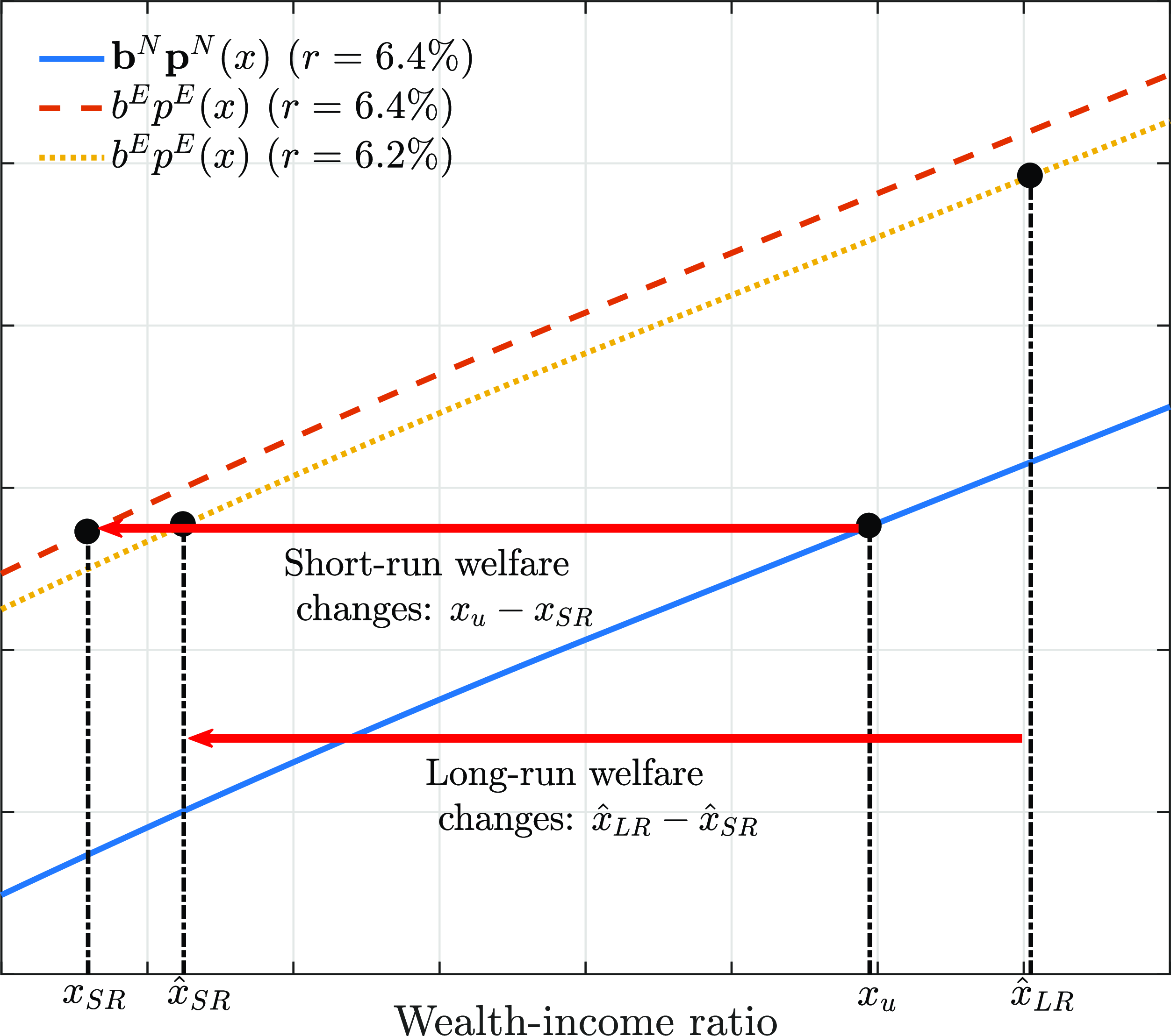
Figure 2 provides a graphical illustration of the welfare changes of removing present bias. Take the naive household as an example. The short-run welfare changes are captured by
 $\omega ^N_{PB}=x_u-x^{SR}$
, where the household values are equivalent,
 $\mathbf{b}^N\mathbf{p}^N(x_u)=b^Ep^{E}(x^{SR})$
.
Additionally, to compare the welfare in the economy without present bias and the economy with heterogenous present bias, we include the following two long-run impacts from present bias removal. On the one hand, more precautious consumption changes the wealth status. On the other, the shift in overall wealth distribution changes the equilibrium interest rate. As a result, the naive household’s wealth-income ratio moves to
 $\hat{x}^{LR}$
on the yellow dotted line (with a different
 $r$
). Since the value of exponential-discounting households on the yellow dotted line is the same as that of naive households on the solid blue line when
 $x=\hat{x}^{SR}$
, the maximum transfer a naive household is willing to pay is
 $\Delta x^N_{PB}=\hat{x}^{LR}-\hat{x}^{SR}$
, such that:
 \begin{equation} \mathbf{b}^N\mathbf{p}^N(x_u)=b^Ep^{E}\left(\hat{x}^{LR}-\Delta x^N_{PB}\right). \end{equation}
Similarly, we can compute the long-run welfare changes by removing sophisticated present bias
 $\Delta x^S_{PB}$
. More important, we consider the distribution of households when analyzing their welfare changes. The long-run welfare changes are reflected by the distribution of
 $\Delta x^j_{PB}$
.
6.1. Welfare analysis of present bias
Short-run welfare changes from removing present bias. The left panel displays the short-run impacts of removing present bias for naive households. The right panel depicts the welfare changes of removing present bias for sophisticated households (
 $\beta ^S=0.98$
). In the left panel, the steady-state wealth-income ratios are
 $\tilde x_{\beta ^N=0.783}=-0.11$
and
 $\tilde x_{\beta ^N=0.88}=2.36$
. The interest rate is fixed at
 $r=6.2\%$
. Other parameter values are provided in Table 1.

Figure 3 depicts the short-run welfare changes (i.e., with a fixed interest rate
 $r$
) from removing present bias
 $\omega ^j_{PB}(x)$
against the wealth-income ratio
 $x$
, where
 $j\in \{S,N\}$
. Two observations can be drawn from the figure. First, when the interest rate is fixed, removing present bias is always beneficial for both naifs and sophisticates, since
 $\omega ^j_{PB}(x)\gt 0$
holds for any given
 $x$
. Second, the welfare gains
 $\omega ^j_{PB}(x)$
increase with the wealth-income ratio
 $x$
. To understand this result, note that equation (21) shows that the higher
 $x$
is, the higher the level of overconsumption induced by present bias. As a result, present-biased households with a larger wealth-income ratio can benefit more from restraining stronger overconsumption incentives. These results are robust with varying values of
 $\beta ^N$
.
We now proceed to explore the long-run impacts of present bias removal. Figure 4 depicts the CDF of long-run welfare changes in the naive and sophisticated cases
 $\Phi ^j(\Delta x^j_{PB})$
.
Long-run welfare changes from removing present bias. The left panel displays the long-run welfare changes of removing present bias for naive households, and the right panel displays the long-run welfare changes of removing present bias for sophisticated households (
 $\beta ^S=0.98$
). In the left panel, the steady-state wealth-income ratios are
 $\tilde x_{\beta ^N=0.783}=-0.085$
and
 $\tilde x_{\beta ^N=0.88}=4.24$
. Other parameter values are provided in Table 1.

Consider first the naive case. Panel A of Figure 4 states that when the degree of present bias is relatively small, removing naive present bias even results in welfare costs, as manifested by
 $\Delta x^N_{PB}\lt 0$
. This result can be explained as the interaction of the following two competing effects. On the one hand, removing households’ present bias directly strengthens their incentives to save. On the other hand, the resulting stronger saving motives raise the capital supply in the economy; to stimulate the firm’s demand for capital and clear the asset market, the equilibrium interest rate
 $r$
must decrease. For instance, with
 $\beta ^N=0.783$
, removing naive present bias decreases the equilibrium interest rate to
 $6.2\%$
from
 $6.4\%$
. The lower interest rate in turn makes saving less appealing. With severe present bias, all households’ overconsumption incentives are sufficiently strong that they are indebted; in this situation, the additional saving motive dominates, and removing naive present bias is always beneficial (see the solid blue line in Panel A of Figure 4). If, in contrast, with mild present bias, most naive households have positive saving rates, the lower interest rate induced by the interest rate channel undermines their saving incentives, thus leading to welfare costs (see the red dashed and yellow dotted lines in Panel A of Figure 4). With
 $\beta ^N=0.88$
, approximately
 $18.75\%$
of naive households suffer from welfare losses after removing their present bias.
Consider next the sophisticated case. As shown in Panel B of Figure 4, removing sophisticated present bias also generates a negative externality on households’ welfare. The economic intuition is the same as in Panel A of Figure 4. Specifically, removing present bias alleviates the scarcity of capital; the resulting decrease in the interest rate
 $r$
limits the return from holding wealth. Since weaker wealth accumulation incentives partially offset the benefit of removing present bias, more than
 $55\%$
of the sophisticates lose welfare in the long run (see the solid blue line in Panel B of Figure 4). This finding shares similar insights with Guiso et al. (Reference Guiso, Pozzi, Tsoy, Gambacorta and Mistrulli2022), in which they incorporate present bias heterogeneity in a mortgage market and show that reducing the present bias of one group harms the welfare of others. Moreover, a higher value of
 $\beta ^N$
mitigates the negative effects on sophisticates’ welfare, as the drop in the interest rate
 $r$
is less drastic.
6.2. Value of sophistication
Sophistication value. The left and right panels depict short- and long-run welfare changes of removing naivete, respectively, where the superscript
 $j\in \{N,S\}$
. Under naive beliefs, the steady-state wealth-income ratios are
 $\tilde x_{\beta ^N=0.783}=-0.085$
,
 $\tilde x_{\beta ^N=0.8}=-0.053$
, and
 $\tilde x_{\beta ^N=0.82}=-0.023$
; under sophisticated beliefs, the steady-state wealth-income ratios are
 $\tilde x_{\beta ^S=0.783}=-0.071$
,
 $\tilde x_{\beta ^S=0.8}=-0.04$
, and
 $\tilde x_{\beta ^S=0.82}=-0.01$
.

Similar to the definition of welfare changes from present bias removal (42), we define the welfare changes of removing naivete,
 $\mathcal{W}_{NS}$
, as the maximum transfer a naive household is willing to pay to become sophisticated:
 \begin{eqnarray} \mathbf{b}^{N}\mathbf{P}^N\left (X_u,Y_u\right )= \mathbf{b}^{S}\mathbf{P}^S\left (X_u-\mathcal{W}_{NS},Y_u\right ), \end{eqnarray}
and the scaled welfare changes of removing naivete
 $\omega _{NS}$
is obtained by solving:
 \begin{eqnarray} \mathbf{b}^{N}\mathbf{p}^N\left (x_u\right )= \mathbf{b}^{S}\mathbf{p}^S\left (x_u-\omega _{NS}\right ). \end{eqnarray}
The short- and long-run welfare changes of removing naivete are captured by
 $\omega _{NS}$
and
 $\Delta x_{NS}$
, respectively.
Suppose that naive households become sophisticated. Figure 5 displays the welfare changes of removing naivete under three different levels of the present bias parameter. It is evident from this figure that removing naivete generates welfare gains:
 $\omega _{NS}(x)\gt 0$
and more than
 $95\%$
of naive households still benefit in the long run. Intuitively, compared to naive households, sophisticates correctly anticipate future selves’ splurging motives and thus save more to prevent potential poverty in the future. For example, with
 $\beta ^j=0.82$
, removing naivete raises the steady-state wealth-income ratio by
 $0.013$
. Moreover, a smaller degree of present bias reduces the sophistication value, as manifested by smaller welfare gains.
6.3. Potential remedies for present bias
Although welfare gains from removing present bias and naivete are substantial for indebted households, it is challenging to implement commitment devices in the first place. To guard against self-control problems and promote savings, prior studies suggest that illiquidity serves as a powerful commitment device, such as illiquid retirement accounts (Beshears et al. Reference Beshears, Choi, Laibson, Madrian and Milkman2015; Beshears et al. Reference Beshears, Choi, Laibson, Madrian and Skimmyhorn2022) and illiquid private equity investment (Acharya et al. Reference Acharya, Jimenez Gomez, Rachinskii and Rivera2022). However, the usage of such commitment devices is limited, and their effectiveness has been called into question. For instance, Beshears et al. (Reference Beshears, Choi, Laibson, Madrian and Skimmyhorn2022) find that present-biased agents spend some or all of their new savings shortly after they separate from each employer. In this section, we explain how to mitigate the negative impacts of present bias and naivete with illiquid investment in human capital and borrowing cost penalty.
6.3.1. Illiquidity
To study the value of illiquidity, we incorporate a linear investment decision. Specifically, given an investment policy
 $i_t\in \{0,\bar{i}\}$
, the household’s labor income in the normal regime,
 $Y_t$
, evolves according to:
 \begin{eqnarray} \frac{dY_t}{Y_t}=\left (\mu +i_t\right ) dt+\sigma d\mathcal{B}_t, \end{eqnarray}
and the process in the default regime is still given by equation (6). The above equation (47) shows that if the household chooses illiquid investment, that is,
 $i_t=0$
, income grows at the rate
 $\mu$
as before. If the household prefers liquid investment by choosing
 $i_t=\bar{i}\gt 0$
, the income growth rate increases. Simultaneously, the household must pay the investment costs; thus, the household’s saving rate,
 $G^{inv}(X_t,Y_t)$
, is given by:
 \begin{eqnarray} G^{inv}(X_t,Y_t)=(r+\lambda +w^{r}\unicode{x1D7D9}_{\{X_{t}\lt 0\}}) X_t+\left (1-\theta i_t\right )Y_t-C^{inv}_t, \end{eqnarray}
where
 $C^{inv}_t$
is the consumption rate in the presence of liquid investment. The parameter
 $\theta \gt 0$
measures the degree of investment costs, and a larger
 $\theta$
denotes the illiquidity of human capital investment.
Proposition 3 (Optimal investment policy for present-biased households). For the type-
 $j$
household, the optimal investment policy is given by:
 \begin{eqnarray} i^j(x)=\left \{ \begin{array}{r@{\quad}c@{\quad}l} 0, &{\text{if }\ F^{j}(X,Y)\gt F^{j,inv}(X,Y)}\\[3pt] \overline{i}, &{\text{if }\ F^{j,inv}(X,Y)\gt F^j(X,Y)} \end{array}\right . \end{eqnarray}
Proof. All proofs are provided in Appendix D.
The economic intuitions for Proposition3 are as follows. In equation (49),
 $F^j(X,Y)$
denotes the value function when the agent chooses illiquid investment and
 $F^{j,inv}(X,Y)$
represents the value function when the agent chooses liquid investment. When the investment cost parameter is low (
 $\theta =3$
) so that the value in the case of liquid investment is higher, that is,
 $F^{j,inv}(X,Y)\gt F^j(X,Y)$
, the agent prefers liquid investment. If, in contrast,
 $\theta$
is so large (
 $\theta =15$
) that
 $F^j(X,Y)\gt F^{j,inv}(X,Y)$
, the agent turns to illiquid investment.Footnote 11
Effects of illiquidity. Panels a and B depict the optimal consumption and probability density function of wealth, respectively. Panels C and D display the CDF of the long-run welfare changes from removing naive present bias and naivete, respectively. Solid blue lines represent the case with liquid investment, and red dashed lines represent the case with illiquid investment. The present bias parameter is set to
 $\beta ^j=0.783$
, and the liquid investment parameter is set to
 $\bar{i}=0.13\%$
, where
 $j\in \{N,S\}$
. Other parameters are reported in Table 1.

Since illiquidity impedes consumption smoothing, the consumption-income ratio drops when
 $\theta$
increases in the short run, as portrayed by Panel A of Figure 6. Panel B of Figure 6 depicts the probability density function of wealth. As can be seen, illiquid investment moves the wealth distribution rightward. The economic intuitions are that illiquid investment weakens households’ borrowing incentives to finance their investment in human capital. Consequently, they have stronger saving motives and reduce their indebtedness level.
Next, we show how illiquidity alters the welfare changes. Panel C of Figure 6 shows that illiquidity reduces the welfare gains from removing naive present bias. This result is straightforward: as mentioned above, illiquidity curbs the present-biased households’ overconsumption incentives (see Panel A of Figure 6) and, thus, weakens the gains from present bias removal. Moreover, Panel D of Figure 6 reflects that incorporating illiquidity decreases the sophistication value, which indicates that illiquidity partially substitutes for the role of sophistication in curbing excessive borrowing.Footnote 12
Effects of borrowing wedge. Panel A depicts the optimal consumption-income ratio for three different levels of the borrowing wedge. Panels B and C display the welfare changes from removing naive present bias and naivete, respectively. The present bias parameters are set to
 $\beta ^N=\beta ^S=0.783$
. Other parameter values are reported in Table 1.

6.3.2. Borrowing wedge
Under the premise of present-biased preferences, the borrowing wedge plays a vital role in affecting households’ welfare. Suppose that the government lowers the borrowing wedge
 $w^r$
. The impacts of a smaller
 $w^r$
depend on the following tradeoff. On the one hand, cheaper credit supply (i.e., a smaller
 $w^r$
) alleviates financial constraints, which enables households to better smooth consumption and insure themselves against financial shocks. As illustrated in Panel A of Figure 7, in the short run, consumption increases after the borrowing wedge narrows. On the other hand, the smaller steady-state wealth-income ratios imply that the flexibility benefits induced by a smaller
 $w^r$
strengthen households’ incentives to borrow, thus incurring a higher indebtedness level.Footnote 13 In other words, cutting the borrowing penalty (i.e., financial deregulation) generates a debt-financed short-run consumption boom at the expense of indebted demand in the future (Mian et al. Reference Mian, Straub and Sufi2021). Panel B of Figure 7 shows that as the borrowing wedge
 $w^{r}$
increases, removing present bias turns out to be less attractive. Moreover, Panel C of Figure 7 shows that although a higher
 $w^r$
reduces the share of households who suffer welfare costs from naivete removal, it lowers the welfare gains from removing naivete. These results indicate that raising the borrowing wedge can help curb households’ overconsumption incentives and thus alleviate the negative impacts of present bias and naivete.
Relatedly, Maxted (Reference Maxted2023) emphasizes that self-imposed commitment devices are difficult to implement because the inflexibility hampers consumer welfare, and he terms this phenomenon the “present-bias dilemma”. This result coincides with short-run welfare effects in our paper. Furthermore, our analysis shows that commitment devices generate substantial welfare gains in the long run. Maxted (Reference Maxted2023) suggests that a consumption tax can restrict overconsumption and redistribute tax revenues back to consumers. In a similar vein, our results imply that government interventions can address the “present-bias dilemma” by partially frontloading long-run welfare improvement to compensate for short-run welfare losses.
7. Conclusion
Heterogeneous present bias among households is a prominent feature in empirical research, but this force is understudied in economics. To shed more light on this matter, we investigate preference heterogeneity and its economic consequences. The interaction of present bias and market incompleteness of uninsurable income risk endogenously generates within-individual patience heterogeneity. Heterogeneous present bias leads to preference heterogeneity across consumers. These features help resolve the intrinsic tension in heterogeneous-agent models. Unlike other models, our one-asset heterogeneous-agent model can simultaneously match the estimates of both the average MPC and key statistics of the wealth distribution. Based on this heterogeneous present bias model, we show that removing present bias benefits indebted households the most, but the resulting lower interest rate harms other households due to dissaving motives. Finally, we find that higher borrowing costs and illiquidity both discipline borrowing incentives and counteract the welfare loss from present bias and naivete.
Our findings suggest several avenues for future research. For instance, we assume away the correlation between present bias and labor income (Lockwood, Reference Lockwood2020). Further exploring the channel through which present bias endogenously changes the labor supply might further amplify the distributional impact of present bias. Moreover, illiquid assets, such as houses, might generate commitment value for consumers with self-control problems (Attanasio et al. Reference Attanasio, Kovacs and Moran2020). If such an illiquid asset is included in our model, is the illiquidity premium more realistic than required in other models?
Acknowledgments
Jinqiang Yang acknowledges the support from the National Natural Science Foundation of China (#72072108; #72342021; #72425012); Siqi Zhao acknowledges the support from the National Natural Science Foundation of China (#72121002; #72371078); Yuan Li acknowledges the support from the Fundamental Research Funds for the Central Universities (#CXJJ-2023-312).
Appendix
A. Proof of Proposition1
This section mainly provides proof for Proposition1.
A.1. Exponential agents
We start by solving for the case with exponential discounting. In the normal regime, the value function
 $F^E(X,Y)$
satisfies the following Hamilton–Jacobi–Bellman (HJB) equation:
 \begin{eqnarray} \begin{split} (\rho +\lambda )F^E(X,Y)=\max _{C^E} \left \{\begin{array}{l@{\quad}c} U(C^E) +G^E(X,Y)F^E_X(X,Y) \\[5pt]+\mu YF^E_Y(X,Y)+\frac{\sigma ^2}{2}Y^2F^E_{YY}(X,Y) \end{array}\right \}. \end{split} \end{eqnarray}
Differentiating the above HJB equation (A.1) with respect to
 $C^E$
, we can obtain the consumption optimality condition (13).
Similar to (17), we assume that the value function
 $F^E(X,Y)$
takes the following form:
 \begin{eqnarray} F^E(X,Y)=\frac{\left (b^EP^E(X,Y)\right )^{1-\gamma }}{1-\gamma }. \end{eqnarray}
Plugging (A.2) into (A.1) and applying the homogeneity property generates the ODE given in (22). To solve for the constant
 $b^E$
, consider the case with an infinite wealth-income ratio
 $x\rightarrow \infty$
; then, we substitute
 $\lim _{x\rightarrow \infty }p^E(x)=x+q$
into the ODE (22) and obtain the following expression for
 $b^E$
:
 \begin{eqnarray} b^E=\left (r+\lambda +\frac{\rho -r}{\gamma }\right )^{\gamma /(\gamma -1)}. \end{eqnarray}
Finally, we demonstrate the relationship between the instantaneous MPC and endogenous risk aversion given in (34). Taking the derivative of the consumption-income ratio
 $c^E(x)$
given in (21) with respect to
 $x$
yields
 \begin{eqnarray} \begin{split} c^{E^{\prime}}(x)=&\left (b^E\right )^{1-1/\gamma }\left [\left (p^{E^{\prime}}(x)\right )^{1-1/\gamma } -p^{E}(x)\frac{\left (p^{E^{\prime}}(x)\right )^{-1/\gamma -1}p^{E^{\prime\prime}}(x)}{\gamma }\right ] \\[5pt]&=\left (b^E\right )^{1-1/\gamma }\left (p^{E^{\prime}}(x)\right )^{-1/\gamma }\left [p^{E^{\prime}}(x)-\frac{p^{E}(x)p^{E^{\prime\prime}}(x)}{\gamma p^{E^{\prime}}(x)} \right ]. \end{split} \end{eqnarray}
According to the definition of endogenous risk aversion in (34), we have:
 \begin{eqnarray} \frac{\gamma ^E_{e}(x)}{\gamma }=p^{E^{\prime}}(x)-\frac{p^{E}(x)p^{E^{\prime\prime}}(x)}{\gamma p^{E^{\prime}}(x)}. \end{eqnarray}
Plugging (A.5) into (A.4) yields (34) under exponential discounting. The complete-markets MPC is equal to
 $m^E=\left (b^E\right )^{1-1/\gamma }=r+\lambda +\frac{\rho -r}{\gamma }$
.
A.2. Sophisticated agents
Now, we turn to the case in which the agent is sophisticated. In the normal regime, we assume that the sophisticated agent anticipates that her future selves will choose consumption strategy
 $\hat C^S$
. Let
 $C\left (\hat C^S\right )$
denote the sophisticated agent’s optimal consumption policy provided that her future selves choose
 $\hat C^S$
. A stationary MPE implies that
 \begin{eqnarray} C\left (\hat C^S\right )=\hat C^S=C^S, \end{eqnarray}
which shows that the current self’s optimal consumption policy is
 $C^S$
provided that all future selves will also choose
 $C^S$
. The optimization problem solved by this (arbitrary) current self is given by:
 \begin{eqnarray} \max _{C^S} U(C^S)dt+\underbrace{\beta G^S(X,Y)F^S_X(X,Y)dt+\beta \mu YF^S_Y(X,Y)dt+\beta \frac{\sigma ^2}{2}Y^2F^S_{YY}(X,Y)dt}_{\beta \mathbb{E}_t\left [dF_t^S(X_t,Y_t)\right ]}. \end{eqnarray}
Solving this (local) optimization problem yields the sophisticated optimality consumption condition given in equation (12) that
 $U^{\prime}(C^S)=\beta F^S_X(X,Y)$
. Substituting this condition into the Bellman equation (11) and then using the model’s scale-invariance property, we can obtain the following ODE for the scaled CEW
 $p^S(x)$
:
 \begin{eqnarray} \begin{split} &\left [\frac{(\beta +\gamma -1)\beta ^{-1/\gamma }\left (b^Sp^{S^{\prime}}(x)\right )^{1-1/\gamma } }{1-\gamma }-\frac{\rho +\lambda }{1-\gamma }+\mu -\frac{\gamma \sigma ^2}{2}\right ]p^S(x) +\frac{\sigma ^2x^2}{2}p^{S^{\prime\prime}}(x) \\&+\left [1-\frac{\gamma \sigma ^2x^2}{2}\frac{p^{S^{\prime}}(x)}{p^S(x)} +\left (r+\lambda +w^r{\unicode{x1D7D9}}_{\{x\lt 0\}}-\mu +\gamma \sigma ^2\right )x\right ]p^{S^{\prime}}(x)=0, \end{split} \end{eqnarray}
which is subject to the following boundary conditions:
 \begin{eqnarray} p^S(\underline{x})=\kappa \hat p^E, \lim _{x\rightarrow \infty }p^{S}(x)=x+q. \end{eqnarray}
From the second equation in (A.9) and the ODE (A.8), we can deduce the expression for
 $b^S$
as follows:
 \begin{eqnarray} b^S=\left [\frac{\rho -r+(r+\lambda )\gamma }{\beta +\gamma -1}\beta ^{1/\gamma }\right ]^{\gamma /(\gamma -1)}. \end{eqnarray}
Next, we demonstrate the relationship
 $c^S(x)=\frac{\gamma }{\gamma +\beta -1}c^E(x)$
given in equation (21). We start by computing the sophisticates’ optimal consumption-income ratio. Substituting the form of
 $F^S(X,Y)$
into the sophisticated consumption optimality condition (21) yields:
 \begin{eqnarray} c^S(x)=\beta ^{-1/\gamma }\left (b^S\right )^{1-1/\gamma }p^S(x)\left (p^{S^{\prime}}(x)\right )^{-1/\gamma }. \end{eqnarray}
From equations (A.3) and (A.10), we can infer that
 \begin{eqnarray} (\beta +\gamma -1)\beta ^{-1/\gamma }\left (b^S\right )^{1-1/\gamma } =\rho -r+(r+\lambda )\gamma =\gamma \left (b^E\right )^{1-1/\gamma }. \end{eqnarray}
Applying the above equation to the ODE (A.8), we find that in the normal regime, the scaled CEW for sophisticated agents is equivalent to that for exponential discounters, regardless of the degree of present bias
 $\beta$
. Plugging
 $p^S(x)=p^E(x)$
and (A.12) into (A.11) generates the equation
 $c^S(x)=\frac{\gamma }{\gamma +\beta -1}c^E(x)$
as desired.
The proof of the relationship between the instantaneous MPC and endogenous risk aversion is similar to equations (A.4)–(A.5), and the complete-markets MPC under sophistication is
 $m^S=\beta ^{-1/\gamma }\left (b^S\right )^{1-1/\gamma }=\frac{\rho -r+(r+\lambda )\gamma }{\beta +\gamma -1}$
.
A.3. Naive agents
Finally, we consider the case in which the agent is naive. Similar to (A.7), in the normal regime, the optimization problem solved by the naive agent is given by:
 \begin{eqnarray} \max _{C^N} U(C^N)dt+\beta G^N(X,Y)F^E_X(X,Y)dt+\beta \mu YF^E_Y(X,Y)dt+\beta \frac{\sigma ^2}{2}Y^2F^E_{YY}(X,Y)dt. \end{eqnarray}
Note that
 $F^E(X,Y)$
denotes the perceived continuation-value function, conditioning on the perceived consumption policy
 $C^E(X,Y)$
(see equation (9)). Solving this (local) optimization problem yields the naive consumption optimality condition
 $U^{\prime}(C^N)=\beta F^E_X(X,Y)$
, as given in equation (12). Then, substituting this condition into the Bellman equation (11) and applying the homogeneity property, we can obtain the following ODE for the scaled CEW
 $p^N(x)$
:
 \begin{eqnarray} \begin{split} &\left [\frac{\beta ^{1-1/\gamma }\left (\frac{b^Ep^E(x)}{b^Np^N(x)}\right )^{1-\gamma } \left (b^Ep^{E^{\prime}}(x)\right )^{1-1/\gamma }-(\rho +\lambda )}{1-\gamma }+\mu -\frac{\gamma \sigma ^2}{2}\right ]p^N(x) \\&+\left (r+\lambda +w^r{\unicode{x1D7D9}}_{\{x\lt 0\}}-\mu +\gamma \sigma ^2\right )xp^{N^{\prime}}(x)+\frac{\sigma ^2x^2}{2}p^{N^{\prime\prime}}(x) \\&+\left [1-\beta ^{-1/\gamma }\left (b^Ep^{E^{\prime}}(x)\right )^{1-1/\gamma }\frac{p^E(x)}{p^{E^{\prime}}(x)} -\frac{\gamma \sigma ^2x^2}{2}\frac{p^{N^{\prime}}(x)}{p^N(x)}\right ]p^{N^{\prime}}(x)=0. \end{split} \end{eqnarray}
which is subject to the following boundary conditions:
 \begin{eqnarray} p^N(\underline{x})=\kappa \hat p^E, \lim _{x\rightarrow \infty }p^{N}(x)=x+q. \end{eqnarray}
Plugging the second condition in (A.15) into the above ODE (A.14) yields the following equation for
 $b^N$
:
 \begin{eqnarray} \beta ^{-1/\gamma }\left (b^E\right )^{1-1/\gamma }\left [\beta \left (\frac{b^E}{b^N}\right )^{1-\gamma }+\gamma -1\right ] =\rho -r+(r+\lambda )\gamma, \end{eqnarray}
where the solution of
 $b^N$
is unique.
To calculate
 $c^N(x)$
, we plug the form of
 $F^N(X,Y)$
into the naive consumption optimality condition (12):
 \begin{eqnarray} c^N(x)=\beta ^{-1/\gamma }\left (b^E\right )^{1-1/\gamma }p^E(x)\left (p^{E^{\prime}}(x)\right )^{-1/\gamma } =\beta ^{-1/\gamma }c^E(x), \end{eqnarray}
which is the second equation in (21) as desired.
The proof for the relationship between the instantaneous MPC and endogenous risk aversion is similar to equations (A.4)–(A.5), and the complete-markets MPC under naivete is
 $m^N=\beta ^{-1/\gamma }\left (b^E\right )^{1-1/\gamma }=\beta ^{-1/\gamma }\left (r+\lambda +\frac{\rho -r}{\gamma }\right )$
.
B. Proof of Euler equation
This section mainly shows how to derive the Euler equation for present-biased consumption (35).
B.1. Sophisticated case
Taking a derivative of (11) with respect to the wealth
 $X$
gives:
 \begin{align} (\rho +\lambda )F^S_X(X,Y) & = U^{\prime}(C^S)C^S_X(X,Y) +\left [r+\lambda +w^r{\unicode{x1D7D9}}_{\{X\lt 0\}}-C^S_X(X,Y)\right ]F^S_X(X,Y) \nonumber\\& \quad +G^S(X,Y)F^S_{XX}(X,Y) +\mu YF^S_{YX}(X,Y)+\frac{\sigma ^2}{2}Y^2F^S_{YYX}(X,Y). \end{align}
Using the optimality condition (12) that
 $U^{\prime}(C^S)=\beta F^S_X(X,Y)$
:
 \begin{align} \left [\rho +(1-\beta )C^S_X-r-w^r{\unicode{x1D7D9}}_{\{X\lt 0\}}\right ]U^{\prime}(C^S) & = G^S(X,Y)U^{\prime}(C^S)C^S_X(X,Y) +\mu YU^{\prime}(C^S)C^S_Y(X,Y) \nonumber\\& \quad +\frac{\sigma ^2}{2}Y^2\left [U^{\prime\prime\prime}(C^S)\left (C^S_Y(X,Y)\right )^2+U^{\prime\prime}(C^S)C^S_{YY}(X,Y)\right ]. \end{align}
Applying Ito’s Lemma to
 $U^{\prime}(C^S(X_t,Y_t))$
yields:
 \begin{align} \mathbb{E}\left [dU^{\prime}(C^S(X_t,Y_t))\right ]/dt & = G^S(X,Y)U^{\prime}(C^S)C^S_X(X,Y) +\mu YU^{\prime}(C^S)C^S_Y(X,Y) \nonumber\\& \quad +\frac{\sigma ^2}{2}Y^2\left [U^{\prime\prime\prime}(C^S)\left (C^S_Y(X,Y)\right )^2+U^{\prime\prime}(C^S)C^S_{YY}(X,Y)\right ] \end{align}
Plugging (B.3) into (B.2) yields:
 \begin{eqnarray} \left [\rho +(1-\beta )C^S_X-r-w^r{\unicode{x1D7D9}}_{\{X\lt 0\}}\right ]U^{\prime}(C^S)=\mathbb{E}\left [dU^{\prime}(C^S(X_t,Y_t))\right ]/dt, \end{eqnarray}
which is equation (35) as desired.
B.2. Naive case
The proof in the naive case begins the same as above, except now the agent’s value function is based on their perceived behavior. Thus, taking the derivative of the perceived value function (A.1) with respect to
 $X$
yields:
 \begin{align} (\rho +\lambda )F^E_X(X,Y) & = U^{\prime}(C^E)C^E_X(X,Y) +\left [r+\lambda +w^r{\unicode{x1D7D9}}_{\{X\lt 0\}}-C^E_X(X,Y)\right ]F^E_X(X,Y) \nonumber\\& \quad +G^E(X,Y)F^E_{XX}(X,Y) +\mu YF^E_{YX}(X,Y)+\frac{\sigma ^2}{2}Y^2F^E_{YYX}(X,Y). \end{align}
Applying the optimality condition for naive agents’ true consumption rule (12) that
 $U^{\prime}(C^N)=\beta F^E_X(X,Y)$
yields:
 \begin{align} \left (\rho -r-w^r{\unicode{x1D7D9}}_{\{X\lt 0\}}\right )U^{\prime}(C^N) & = \left [\beta U^{\prime}(C^E)-U^{\prime}(C^N)\right ]C^E_X(X,Y)+G^E(X,Y)U^{\prime}(C^N)C^N_X(X,Y) \nonumber\\&+\mu YU^{\prime}(C^N)C^N_Y(X,Y) \nonumber\\&+\frac{\sigma ^2}{2}Y^2\left [U^{\prime\prime\prime}(C^N)\left (C^N_Y(X,Y)\right )^2+U^{\prime\prime}(C^N)C^N_{YY}(X,Y)\right ]. \end{align}
Note that the optimality condition for the perceived consumption is
 $U^{\prime}(C^E)=F^E_X(X,Y)$
, while
 $U^{\prime}(C^N)=\beta F^E_X(X,Y)$
, we have
 $\beta U^{\prime}(C^E)=U^{\prime}(C^N)$
. The relationship between the drifts of wealth
 $G^E(X,Y)$
and
 $G^N(X,Y)$
is:
 \begin{align} G^E(X,Y) & = \left (r+\lambda +w^r{\unicode{x1D7D9}}_{\{X\lt 0\}}\right )X+Y-C^E(X,Y) \nonumber\\&=\left (r+\lambda +w^r{\unicode{x1D7D9}}_{\{X\lt 0\}}\right )X+Y-C^N(X,Y)+C^N(X,Y)-C^E(X,Y) \nonumber\\&=G^N(X,Y)+C^N(X,Y)-C^E(X,Y), \end{align}
Using these:
 \begin{align} \left (\rho -r-w^r{\unicode{x1D7D9}}_{\{X\lt 0\}}\right )U^{\prime}(C^N)& = +G^N(X,Y)U^{\prime}(C^N)C^N_X(X,Y)\nonumber\\& \quad +\left (C^N-C^E\right )U^{\prime\prime}(C^N)C^N_{X}(X,Y) +\mu YU^{\prime}(C^N)C^N_Y(X,Y) \nonumber\\&\quad +\frac{\sigma ^2}{2}Y^2\left [U^{\prime\prime\prime}(C^N)\left (C^N_Y(X,Y)\right )^2+U^{\prime\prime}(C^N)C^N_{YY}(X,Y)\right ]. \end{align}
The naive true consumption rule
 $c^N(x)=\beta ^{-1/\gamma }c^E(x)$
implies
 $C^E(X,Y)=\beta ^{1/\gamma }C^N(X,Y)$
. Plugging this into (B.8) and using the property that
 $-\gamma =\frac{U^{\prime\prime}(C)C(X,Y)}{U^{\prime}(C)}$
yields:
 \begin{eqnarray} \frac{\mathbb{E}\left [dU^{\prime}(C^N(X_t,Y_t))\right ]/dt}{U^{\prime}(C^N(X_t,Y_t))} =\rho +\gamma \left (1-\beta ^{1/\gamma }\right )C^N_X(X,Y)-r-w^r{\unicode{x1D7D9}}_{\{X\lt 0\}}, \end{eqnarray}
which is equation (35) as desired.
C. Proof of Section 6
This section mainly shows how to compute present-biased households’ value
 $\mathbf{F}^j(X,Y)$
defined in (39), where
 $j\in \{S,N\}$
. Given the type-
 $j$
agent’s optimal consumption policy
 $C^j(X,Y)$
, her value in the normal regime,
 $\mathbf{F}^j(X,Y)$
, satisfies the following differential equation:
 \begin{eqnarray} (\rho +\lambda )\mathbf{F}^j(X,Y)=U^{\prime}(C^j)+G^j(X,Y)\mathbf{F}_X^j(X,Y)+\mu Y\mathbf{F}_Y^j(X,Y)+\frac{\sigma ^2}{2}Y^2\mathbf{F}_{YY}^j(X,Y), \end{eqnarray}
subject to the following value-matching condition at the default threshold:
 \begin{eqnarray} \mathbf{F}^j(\underline{X}_t,Y)=\widehat F^E(\kappa Y). \end{eqnarray}
Plugging the conjectured form (39) into (C.1) and applying the homogeneity property yields the ODE for
 $\mathbf{p}^j(x)$
, as given in (40).
To solve the constant
 $\mathbf{b}^j$
, consider the situation in which
 $x$
goes infinity. Plugging the condition (41) that
 $\lim _{x\rightarrow \infty }\mathbf{p}^j=x+q$
into the consumption policies (21) yields:
 $\lim _{x\rightarrow \infty }c^j=m^j(x+q)$
, where
 $m^j$
is the complete-markets MPC. Then, we substitute these two conditions into (40) and obtain the two equations for
 $\{\mathbf{b}^S, \mathbf{b}^N\}$
:
 \begin{eqnarray} \left (\mathbf{b}^S\right )^{\gamma -1} \left (\frac{\gamma (b^E)^{1-1/\gamma }}{\gamma +\beta -1}\right )^{1-\gamma } -\frac{\beta (b^E)^{1-1/\gamma }}{\gamma +\beta -1}=0, \end{eqnarray}
 \begin{eqnarray} \left (\mathbf{b}^N\right )^{\gamma -1}\left (\eta ^{-1/\gamma }(b^E)^{1-1/\gamma }\right )^{1-\gamma } -\gamma (b^E)^{1-1/\gamma }-(1-\gamma )\left (\eta ^{-1/\gamma }(b^E)^{1-1/\gamma }\right )=0, \end{eqnarray}
where the constant
 $b^E$
is given in (A.3).
D. Proof of Proposition3
This section mainly provides proof of Proposition3. Take the sophisticated case as an example. Similar to the consumption policy (A.6), under a stationary MPE, the current self’s optimal investment policy is
 $i^S$
provided that all future selves will also choose
 $i^S$
. Therefore, under the premise of human capital investment, the value function in the normal regime,
 $F^{S,inv}(X,Y)$
, satisfies the following Bellman equation:
 \begin{align} (\rho +\lambda )F^{S,inv}(X,Y) & = U\left (C^{S,inv}\right )+\left [(r+\lambda +w^{r}\unicode{x1D7D9}_{\{X\lt 0\}}) X+\left (1-\theta{i^S}\right )Y-C^{S,inv}\right ]F^{S,inv}_X(X,Y) \nonumber\\& \quad +(\mu +i^S)YF^{S,inv}_Y(X,Y)+\frac{\sigma ^2}{2}Y^2F^{S,inv}_{YY}(X,Y), \end{align}
and the value function in the default regime does not change (see equations (14) and (24)), as households in this regime cannot afford the investment cost. Under the premise of illiquid investment, the value function
 $F^{S}(X,Y)$
is solved by the Bellman equation (11). Obviously, when
 $F^{S,inv}(X,Y)-F^{S}(X,Y)\gt 0$
, the household can benefit from liquid investment. If, by contrast,
 $F^{S,inv}(X,Y)-F^{S}(X,Y)\lt 0$
, the household suffers value loss from liquid investment. Accordingly, we can obtain the optimal investment policy given in equation (49). Moreover, human capital investment does not directly change the optimality condition for consumption, which is still given by
 $U^{\prime}(C^{S,inv})=\beta F_X^{S,inv}(X,Y)$
; however, it can indirectly affect consumption through the value function
 $F_X^{S,inv}(X,Y)$
.
By applying Ito’s Lemma, the scaled saving rate in the presence of human capital investment is given by:
 \begin{eqnarray} g^{S,inv}(x)=1-\theta i^S(x)+\left (r+\lambda +w^r{\unicode{x1D7D9}}_{\{x\lt 0\}}-i^S(x)+\sigma ^2\right )x -c^{S,inv}(x). \end{eqnarray}
To solve (D.1), we substitute the conjectured form of
 $F^{S,inv}(X,Y)=\frac{\left (b^Sp^{S,inv}(x)\right )^{1-\gamma }}{1-\gamma }Y^{1-\gamma }$
into (D.1) generates:
 \begin{align} &\left [\frac{(\beta +\gamma -1)\beta ^{-1/\gamma }\left (b^Sp^{S,inv^{\prime}}(x)\right )^{1-1/\gamma } }{1-\gamma }-\frac{\rho +\lambda }{1-\gamma }+\mu +i^S(x)-\frac{\gamma \sigma ^2}{2}\right ]p^{S,inv}(x) +\frac{\sigma ^2x^2}{2}p^{S,inv^{\prime\prime}}(x) \nonumber\\&+\left [1-\theta i^S(x) -\frac{\gamma \sigma ^2x^2}{2}\frac{p^{S,inv^{\prime}}(x)}{p^{S,inv}(x)} +\left (r+\lambda +w^r{\unicode{x1D7D9}}_{\{x\lt 0\}}-\mu -i^S(x)+\gamma \sigma ^2\right )x\right ]p^{S,inv^{\prime}}(x)=0. \end{align}
where
 $p^{S,inv}(x)$
denotes the scaled CEW in the presence of liquid investment and the constant
 $b^S$
is given in equation (A.10). The two boundary conditions for the above ODE (D.3) are the same as in (A.9), except that the constant
 $q$
becomes
 $1/(r+\lambda -\mu -i^S)$
. A similar approach can be used in the cases of naivete and exponential discounting.
E. Computing aggregates
In this section, we mainly illustrate how to compute equilibrium objects
 $\{r,w,K,Y_0\}$
by iterating over candidate interest rates. First, given an interest rate
 $r$
, we obtain the average wealth in the economy
 $\mathbb{E}(X)$
by aggregating over the household’s optimal savings demand. Second, according to equations (32) and (33), the wage rate
 $w$
can be expressed as a function of the interest rate
 $r$
, which is given by:
 \begin{eqnarray} w=A(1-\alpha )\left (\frac{r+\delta }{A\alpha }\right )^{\frac{\alpha }{\alpha -1}}. \end{eqnarray}
Third, since endowed labor units
 $H$
are exogenous and the household does not value leisure, the total wage payments equal labor earnings, which is equation (31) as desired. From this equation, we can infer the value of the initial labor earnings
 $Y_0$
.
Fourth, we solve for the aggregate capital stock
 $K$
by using equation (33) that
 $w=A(1-\alpha )\left (K/H\right )^{\alpha }$
, where the labor demand equals labor supply
 $L=H$
. Finally, we check whether the aggregate capital stock
 $K$
obtained in the step
 $4$
equals the average wealth
 $\mathbb{E}(X)$
obtained in the step
 $1$
. If so, we have found a fixed point. Otherwise, we continue the above iteration process until we find one. From a fixed point, we obtain the four equilibrium objects
 $\{r,w,K,Y_0\}$
.



